
A scSE-LinkNet Deep Learning Model for Daytime Sea Fog Detection


College of Oceanography and Space Informatics, China University of Petroleum (East China), Qingdao 266580, China
*
Author to whom correspondence should be addressed.
Remote Sens. 2021, 13(24), 5163; https://0-doi-org.brum.beds.ac.uk/10.3390/rs13245163
Submission received: 1 November 2021
/
Revised: 13 December 2021
/
Accepted: 17 December 2021
/
Published: 20 December 2021
(This article belongs to the Special Issue Explainable Deep Neural Networks for Remote Sensing Image Understanding)
Abstract
:Sea fog is a precarious weather disaster affecting transportation on the sea. The accuracy of the threshold method for sea fog detection is limited by time and region. In comparison, the deep learning method learns features of objects through different network layers and can therefore accurately extract fog data and is less affected by temporal and spatial factors. This study proposes a scSE-LinkNet model for daytime sea fog detection that leverages residual blocks to encoder feature maps and attention module to learn the features of sea fog data by considering spectral and spatial information of nodes. With the help of satellite radar data from Cloud-Aerosol Lidar with Orthogonal Polarization (CALIOP), a ground sample database was extracted from Moderate Resolution Imaging Spectroradiometer (MODIS) L1B data. The scSE-LinkNet was trained on the training set, and quantitative evaluation was performed on the test set. Results showed the probability of detection (POD), false alarm rate (FAR), critical success index (CSI), and Heidke skill scores (HSS) were 0.924, 0.143, 0.800, and 0.864, respectively. Compared with other neural networks (FCN, U-Net, and LinkNet), the CSI of scSE-LinkNet was improved, with a maximum increase of nearly 8%. Moreover, the sea fog detection results were consistent with the measured data and CALIOP products.
1. Introduction
Sea fog is a precarious weather phenomenon that appears when water vapor near the surface is condensed to form suspended water droplets [1]. It can result in the horizontal visibility of sea being less than 1 km and threatens the safety of navigation, aviation, and transportation, which in turn can affect the economy and threaten lives. More than 50 foggy days occur annually over the coast of China, and more than 50% of accidents in the Yellow Sea have happened when experiencing fog [2]. Consequently, effective monitoring and identification of sea fog is crucial for safe navigation and aviation.
In the case of sea fog, human-recorded observations cover only a limited area over a short period of time. Ground stations and buoy stations for sea fog are sparse, meaning there are great limitations in observation frequency, time, and spatial coverage. Earth observation (EO) satellites offer cost-effective and timely images covering large areas with high temporal and spatial resolutions [3]. They have therefore become indispensable technical means for real-time observation of the occurrence, development, and extinction of sea fog. However, daytime sea fog detection is still a significant problem because of the similarity in spectral characteristics of fog and other types of cloud (middle/high level clouds, stratus clouds, and low clouds) [4].
The radiance threshold and brightness temperature differential method [5,6,7,8,9,10,11,12,13] is most commonly used for daytime sea fog detection in national and international scales worldwide. For example, Deng [14] used a multiband threshold method for MODIS data to detect daytime sea fog in the South China Sea and validated it using sea fog observations from the coastal regions. However, the use of a fixed threshold might be inaccurate and inflexible because of the seasonal variation of time. Dynamic thresholds can solve this problem to some extent [15,16,17]. The threshold method is widely used as it is simple and fast. However, the traditional threshold method generally has some problems, such as inaccurate division of cloud and fog in the cloud–fog mixing area and rough extraction of fog and stratus boundaries.
Based on the above problems, it is difficult to accurately distinguish sea fog and cloud in the cloud–fog mixing area with optical satellites because the optical properties between them are similar, especially for sea fog and low stratus. The main difference between sea fog and stratus is whether the cloud base meets the sea surface. Therefore, the most direct and reliable way to distinguish them is to obtain the height of the base of stratus and sea fog. With the ability to observe the vertical structure of the atmosphere, satellite radar data from Cloud-Aerosol Lidar and Infrared Pathfinder Satellite Observations (CALIPSO)/CALIOP can penetrate clouds and aerosols to obtain accurate sea fog. They can be gradually used as auxiliary data combined with the threshold method. CALIOP data is also used to verify sea fog detection results. Wu et al. used measurement data acquired by CALIOP to detect sea fog [18]. Xiao et al. presented an algorithm for daytime sea fog detection over the Greenland Sea based on MODIS and CALIOP data [19]. Wan et al. used CALIOP assisted MODIS data to extract sea fog sample points and analyzed the sea fog spectral response curve from MODIS data [20]. These studies combined CALIOP data with other methods and used CALIOP data to verify sea fog detection results, thereby providing a method to accurately obtain sea fog samples and further determine sea fog and stratus boundaries.
Additionally, a number of studies have taken a different approach for sea fog detection using machine learning. This includes methods such as the expectation maximization algorithm (EM) [21] and decision tree (DT) [22] to precisely differentiate between stratus and sea fog. Although the introduction of machine learning further clarifies the stratus and sea fog boundaries, the process is more cumbersome because of the transformation and visualization of the detection results.
Recently, a few studies have used deep learning method for fog detection. For example, Drönner et al. proposed a novel cloud classification method based on convolutional neural network (CNN) called the cloud segmentation CNN (CS-CNN) [23]. Liu et al. presented a daytime sea fog retrieval model that used fully convolutional networks (FCN) for preprocessing and fully connected condition random field (CFD) for postprocessing [24]. Zhu et al. used the U-Net deep learning model to construct a sea fog detection model for MODIS multispectral images [25]. Jeon et al. proposed an approaching method to identify sea fog by applying a convolution neural network transfer learning (CNN-TL) model [26]. Considering the above methods, sea fog detection can be carried out by judging the category of each pixel in remote sensing images, which involves semantic segmentation of the deep learning method. The multilayer network in the deep learning method can mine data features as much as possible and directly obtain the detection results. The detection accuracy of the deep learning method is significantly better compared to the threshold method and machine learning method. However, due to the few training samples and structural limitations of the neural network, there are still some problems, such as insufficient training of the network and inaccurate division of stratus and sea fog boundaries. There are two problems in the application of deep learning method for sea fog detection: (1) The selection of deep learning samples is greatly affected by subjectivity, especially in the mixed areas of sea fog and clouds. There is lack of real ground object category information, which leads to inaccurate labeling of sea fog and clouds and in turn affects the accuracy of subsequent model training. (2) The number of sea fog samples is small, which leads to poor training effects in large-scale networks. The boundaries of features extracted by conventional semantic segmentation networks are relatively rough.
In this study, we applied MODIS data together with CALIOP vertical feature mask (VFM) products to make a ground truth label that would improve the accuracy of manual sample selection. Then, a scSE-LinkNet deep learning model for daytime sea fog detection was developed in which the LinkNet semantic segmentation backbone was combined with attention mechanism. The model used in this study obtained better detection result with a small sample size dataset. Finally, according to international definitions, fog reduces visibility below 1 km (0.62 miles) [27]. Therefore, we used visibility data which from International Comprehensive Ocean-Atmosphere Data Set (ICOADS) and meteorological station data, and CALIOP VFM products for comparison and validation.
One of the primary contribution of this study is that it determines whether the combined use of MODIS data and CALIOP VFM products improves the accuracy of ground truth label, especially in mixed areas of sea fog and stratus. Another major contribution is the development of a new model called scSE-LinkNet, which combines LinkNet with attention mechanism for sea fog detection. The model can extract effective features from channel and spatial training samples with only a small number of training samples to accurately determine sea fog area.
2. Materials
2.1. Study Area
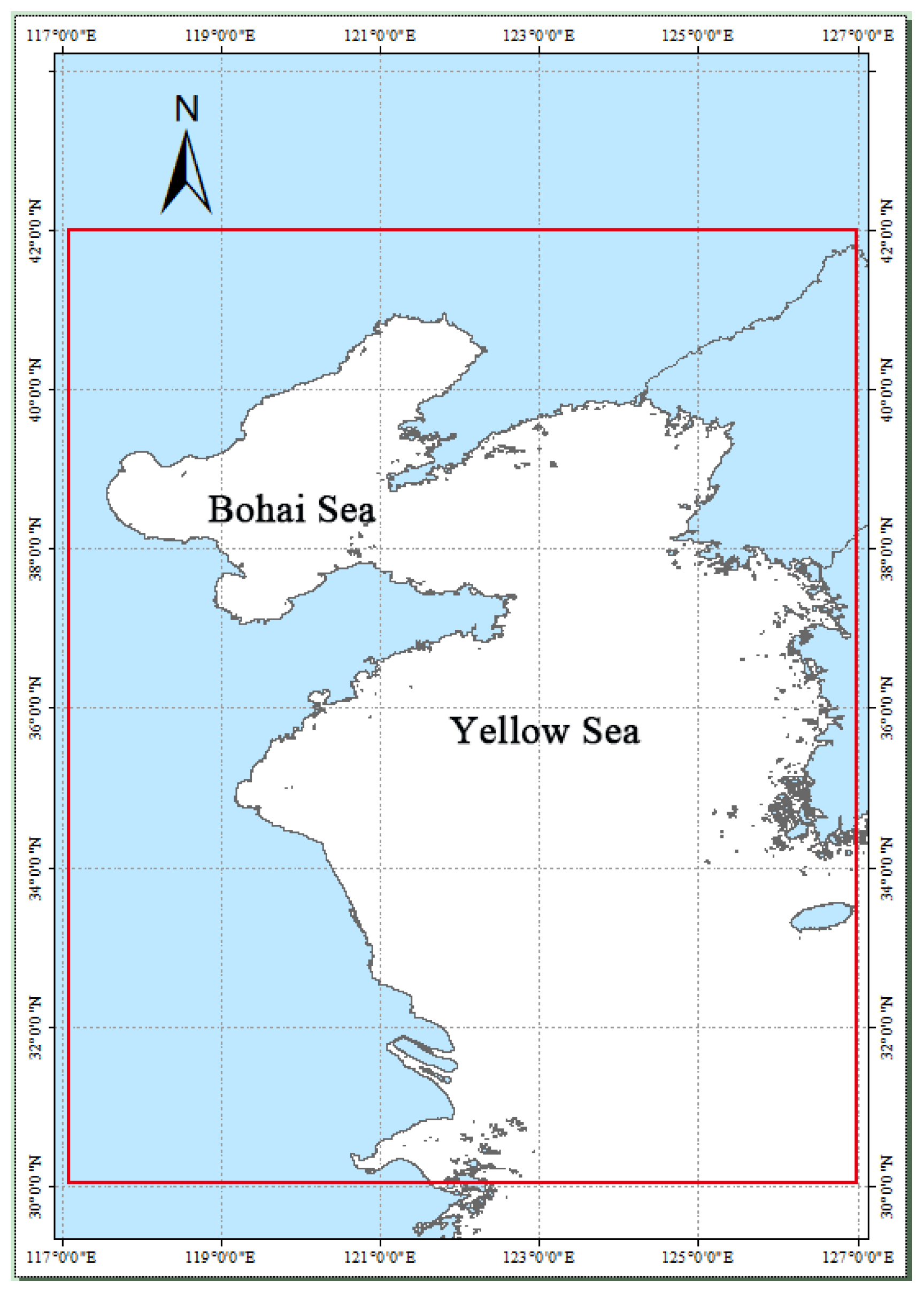
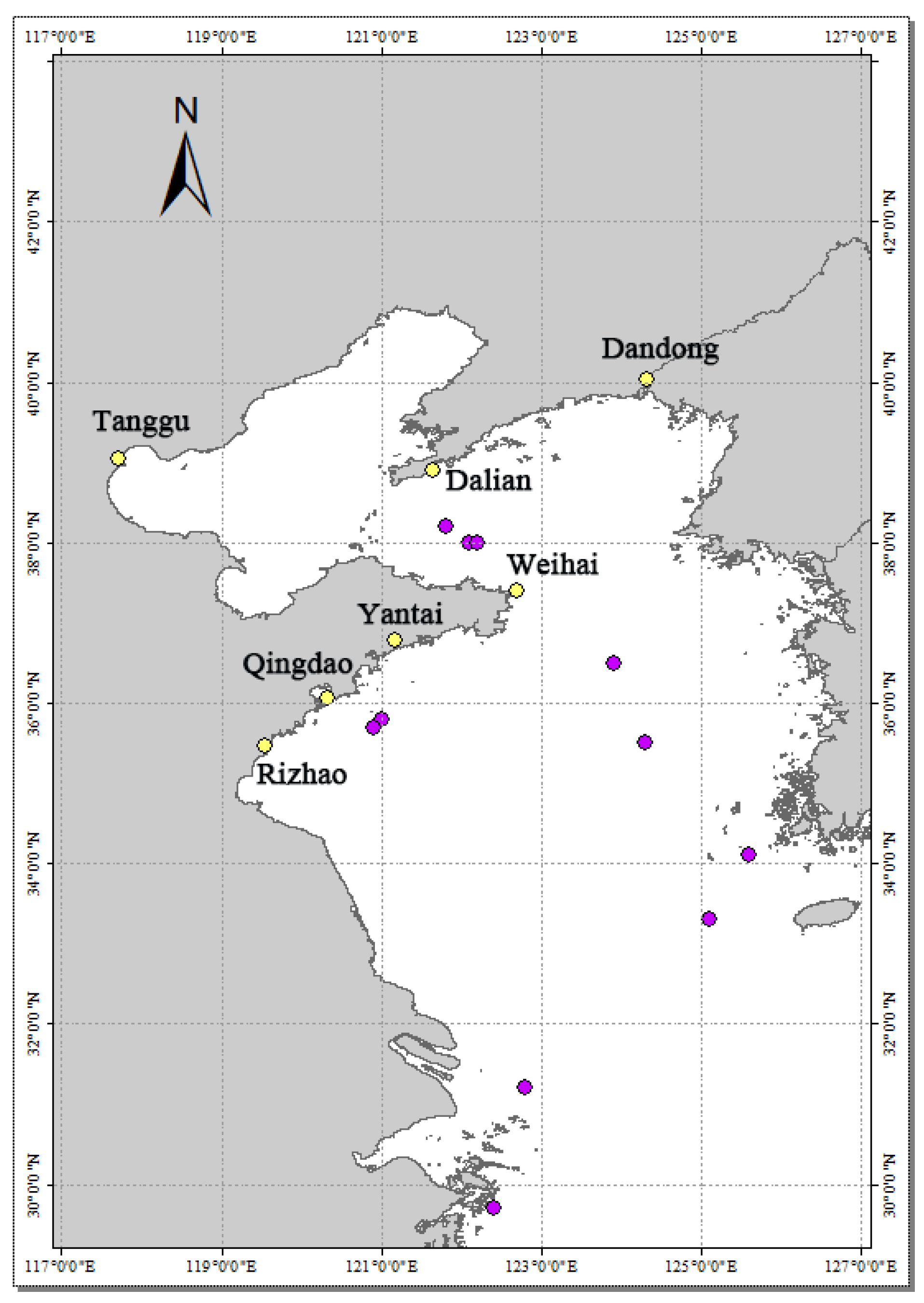
The study area included the Bohai Sea, the Yellow Sea, and their surrounding waters in China. In Figure 1, the red square represents the study area, which ranges between longitudes of 117°E and 127°E and latitudes of 30°N and 42°N. This area sees frequent occurrence of advection fog in spring and summer because the warm moist air over the gulf stream often blows over the colder waters of the sea surface in this region. Fog in the Yellow Sea has a wide distribution range, low atmospheric visibility, and long duration.
2.2. Datasets
Different categories of data were employed in this study, each of which is briefly described below. It should be noted that the fog monitoring report used Chinese Standard Time (CST) time, while the other data used UTC time.
2.2.1. Aqua/MODIS Data
MODIS is one of the Aqua polar orbiting satellite payloads. The spatial resolution with MODIS LIB data is 1 km, with 36 spectral channels ranging from 0.4 to 14.4 μm. We used MYD021KM from version 6.0 and the geolocation product MYD03 from 2016 to 2018, which was obtained from https://ladsweb.modaps.eosdis.nasa.gov/ (accessed on 12 December 2021).
2.2.2. CALIPSO/CALIOP Data
CALIPSO/CALIOP and Aqua/MODIS were both members of the satellite A-Train up to September 2018, with passing times only 1.5 min apart [18], which meant we could obtain accurate type of ground pixels by superimposing two kinds of data. CALIOP data can penetrate clouds and aerosols to obtain vertical profile structure information of the atmosphere. CALIOP Level 2 VFM products describe the vertical structure of the atmosphere, with vertical resolution of 30 m between −0.5 and 8.2 km and horizontal resolution of 333 m, including subsurface, surface, aerosol, clouds, clear air, etc. CALIOP VFM products were downloaded from https://subset.larc.nasa.gov/calipso (accessed on 12 December 2021) to obtain the sample points of sea fog and other sea object samples (including cloud and sea surface samples) to assist manual interpretation of MODIS data.
2.2.3. Fog Monitoring Report
Fog monitoring reports are provided by China Ecological Remote Sensing Information Service Network (CERSISN) based on the fog recognition results of FY series satellite data. They are generally released at 7:30–9:30 (CST time) every morning and include the location and range of fog, which provide a reference for the date of sea fog events. We used fog reports from the time frame 2016 to 2018, and the data were obtained from http://rsapp.nsmc.org.cn/uus/index.jsp/ (accessed on 30 October 2021).
2.2.4. ICOADS Data
ICOADS data is the world’s most extensive surface marine meteorological data collection and can be downloaded from https://icoads.noaa.gov/ (accessed on 12 December 2021). As it contains observations from many different locations, ICOADS underpins a wide range of climate products, including the global surface temperature record, wind, pressure, humidity, clouds, and estimates of air–sea exchange [28]. In addition, we used the visibility data of ICOADS from 2016 to 2018 to validate the sea fog detection results.
2.2.5. Meteorological Station Data
Meteorological station data are provided by China Meteorological Administration and includes visibility data, relative humidity data, dew point temperature data, wind speed and wind direction data. The measured data from meteorological station are hourly observations. We used data from 2016 to 2018. The detailed station information is shown in Table 1.
3. Method
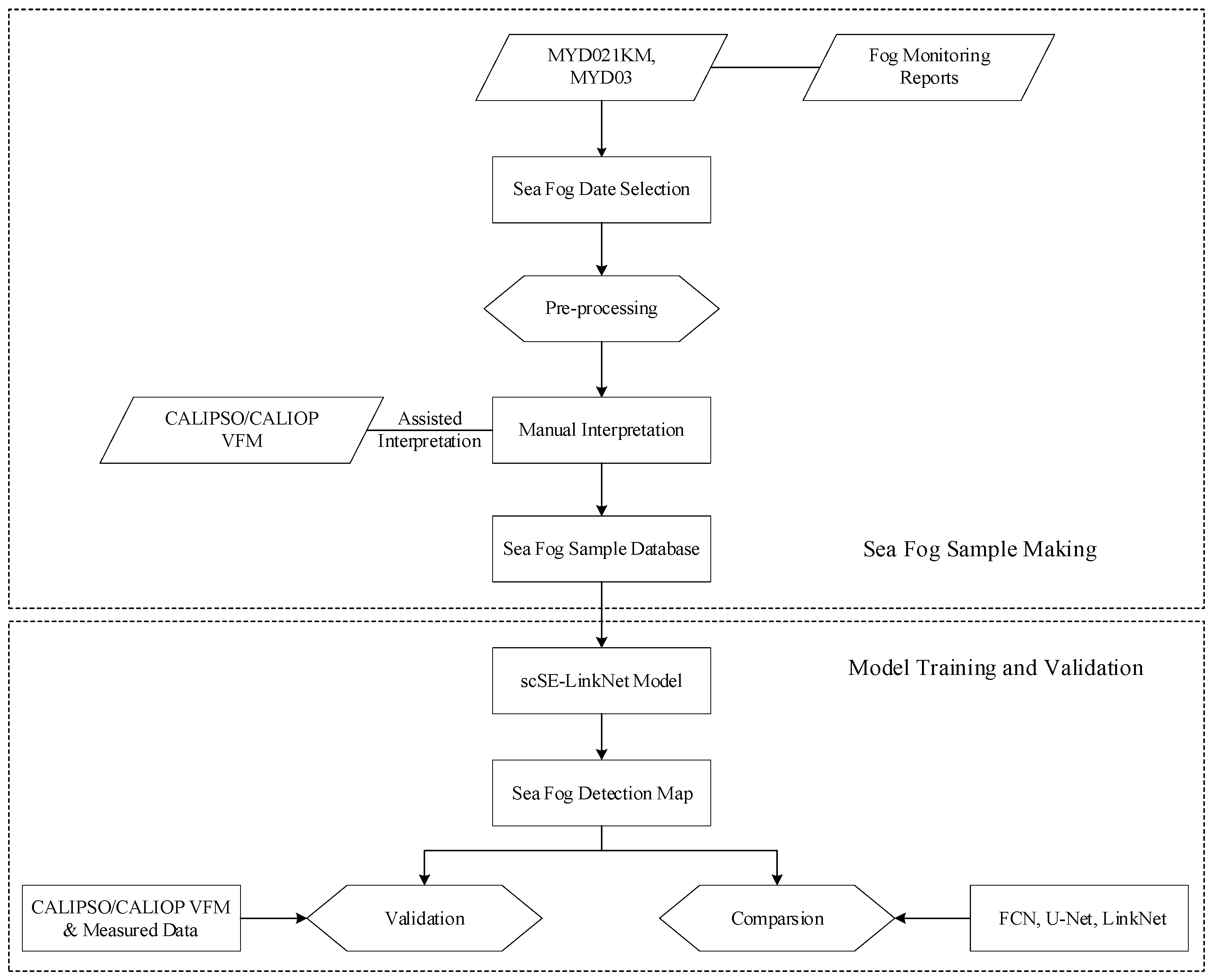
Figure 2 demonstrates a flowchart of the proposed method for daytime sea fog detection, including ground object sample production, model training, and validation. The construction of the scSE-LinkNet deep learning model based on LinkNet and squeeze-and-excitation networks (SENet) is the most important process in this study. The details of each backbone are provided in the following sections.
3.1. LinkNet Backbone
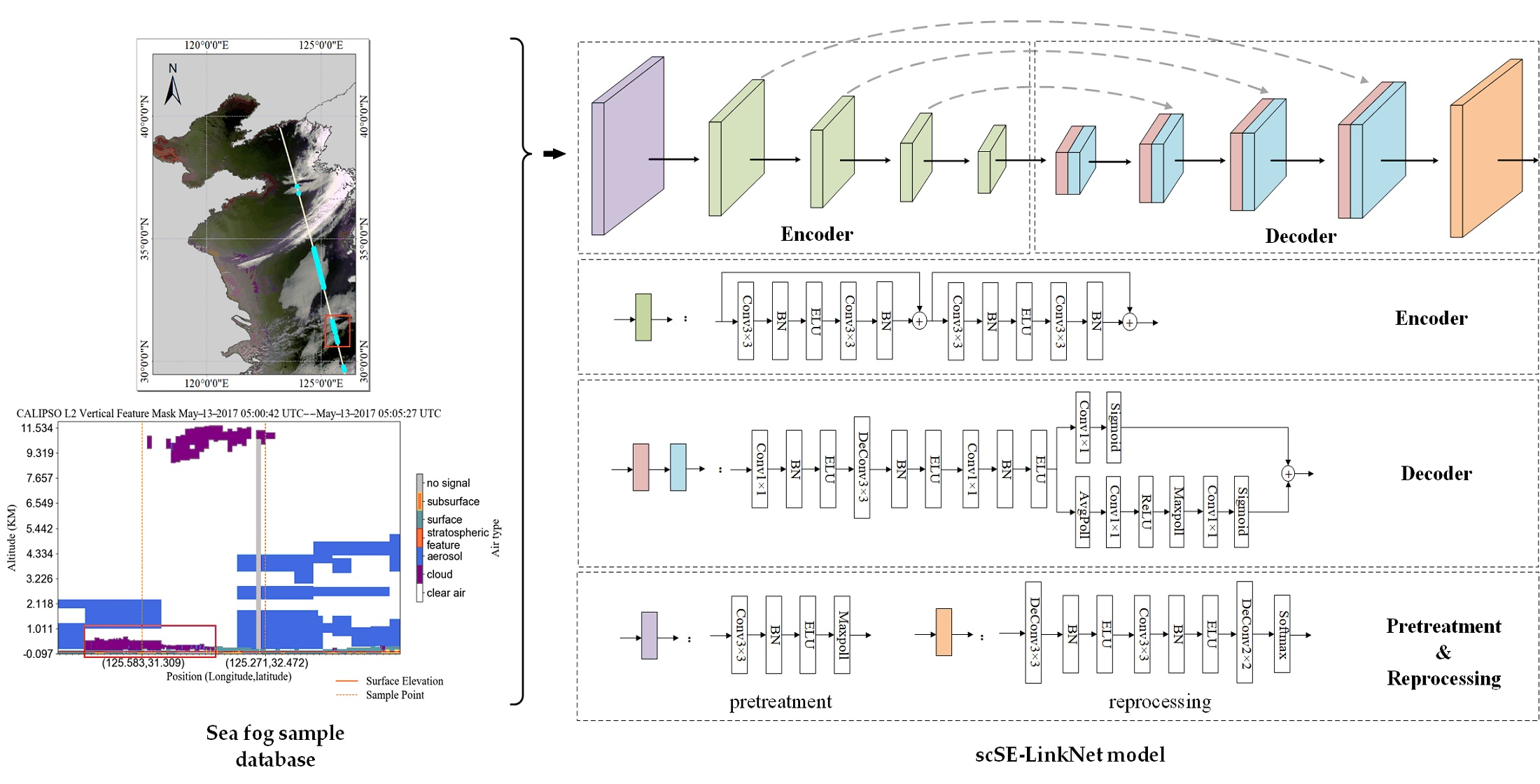
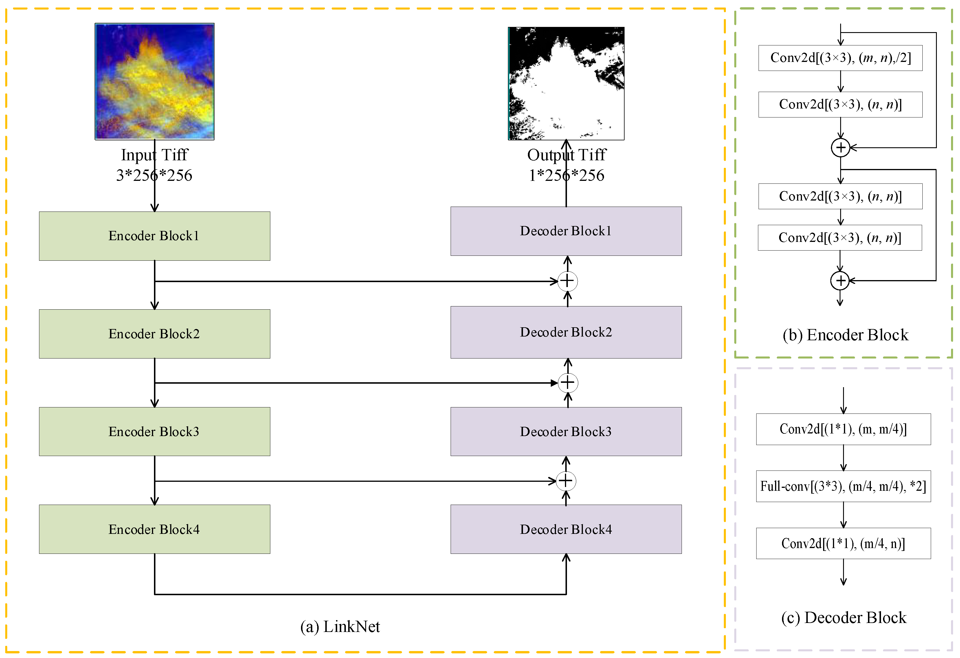
By performing multiple downsampling operations in the encoder of general encoder–decoder networks, some spatial information may lost. It is difficult to recover the lost information using only the downsampled output of the encoder. In this study, we used LinkNet backbone as the basic structure to solve this problem. Compared with the normal convolution, residual network (ResNet) solves the problem caused by the depth of the network during training. LinkNet uses ResNet18 as its encoder, which is a fairly light network. The input of each layer in the encoder is bypassed to the output of its corresponding decoder in LinkNet, which is aimed at recovering lost spatial information that can be used by upsampling operation in the decoder [29]. In addition, LinkNet uses channel reduction scheme to reduce the decoder parameters as the decoder is sharing knowledge learnt by the encoder at every layer. Details of the overall framework is shown in Figure 3. LinkNet uses the residual module to replace the convolution module as its encoder and uses ResNet18 pretraining parameters to optimize network. The decoder of LinkNet uses deconvolution and 1 × 1 convolution kernel to reduce the number of decoder parameters.
3.2. SENet Backbone
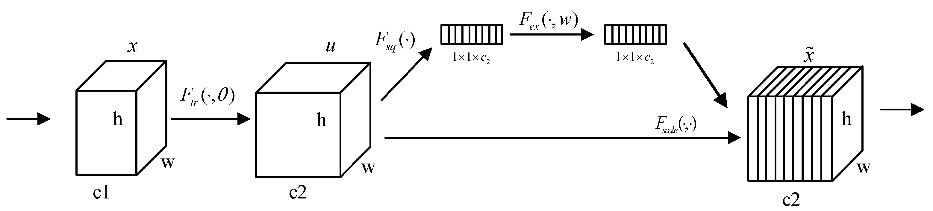
The SENet can be regarded as one of the attention mechanisms. Convolutional neural networks learn a new feature map from the input feature map through the convolution kernel, which is used to fuse more features spatially or to extract multiscale spatial information, such as the multibranch structure of the inception network [30]. For feature fusion of the channel dimensions, the convolution operation defaults to fusion of all channels of the input feature map. The innovation of the SENet is that it pays more attention to the importance of different channels, which means the model can automatically learn to use global information to selectively emphasize informative features and suppress less useful ones. The squeeze-and-excitation (SE) module proposed by SENet is shown in Figure 4.
In Figure 4, is any transformation mapping the input to the feature maps . In one method, the feature first passes through a squeeze operation () and then passes through an excitation operation (), which takes the form of a simple self-gating mechanism. In another method, the feature passes through a scale transformation (). The weights of the two methods can generate the output of the SE block, which can be fed directly into subsequent layers of the network [31].
As the main part of SENet, the SE module performs attention or gating operations on the channel. This attention mechanism pays more attention to the channel with maximum information volume and suppresses the unimportant channel features. The SE module is a universal structure that can be embedded in the existing network architecture.
3.3. scSE-LinkNet Backbone
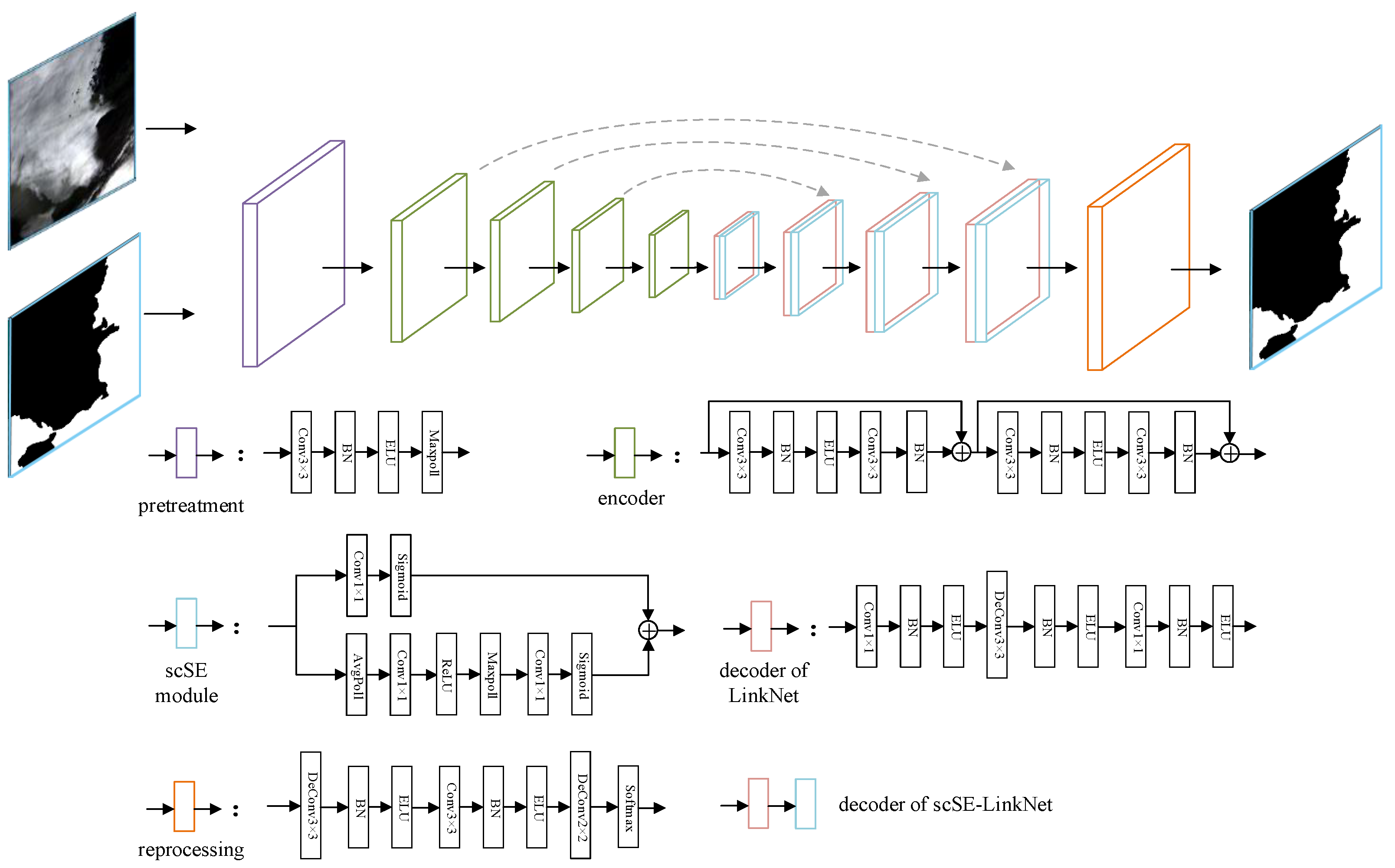
scSE-LinkNet is a model obtained by applying the SE module to the LinkNet (Figure 5). In this study, the scSE module was added to the LinkNet decoding structure by considering the spectral and spatial information of the nodes to improve the model’s ability to extract global information. Using ELU activation function instead of ReLU improves the robustness of the noise and better solves the gradient dispersion problem in the training process. In addition, the focal loss replaces the cross entropy loss, which improves the problem of decreased training accuracy caused by sample imbalance in the training process.
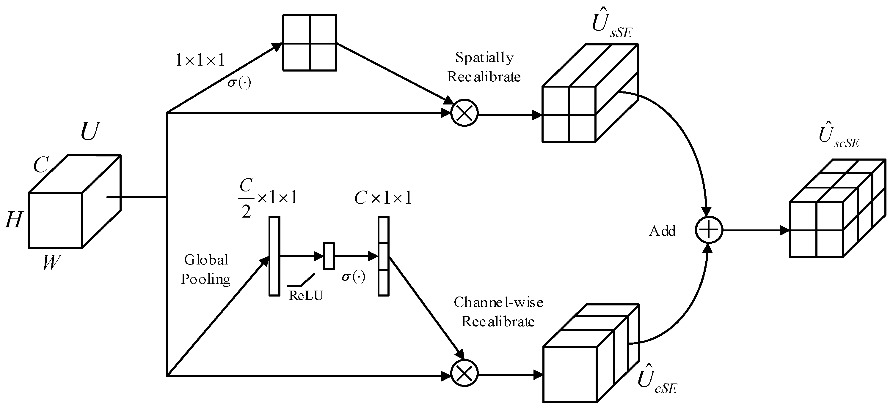
The attention mechanism SE module focuses on the features in spatial and different channels. In this study, we added scSE module in the LinkNet decoding part, including cSE and sSE modules, which enhanced the meaningful features and suppressed useless features in channel and spatial dimensions. The structure of the scSE module is shown in Figure 6.
This recalibration encourages the network to learn more meaningful feature maps, which is relevant both spatially and channel-wise. In this study, we added the scSE block to the decoder of LinkNet (Figure 7).
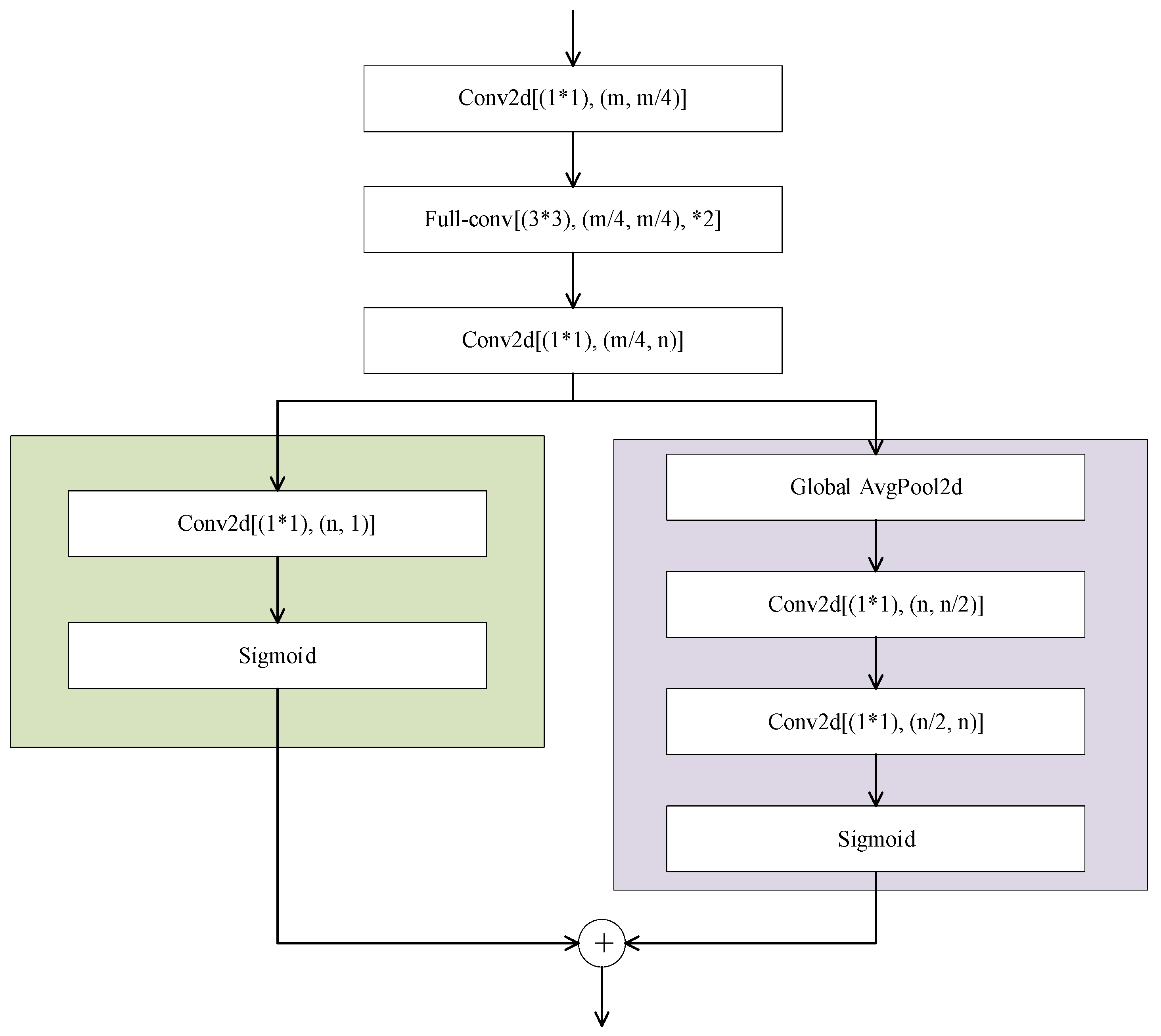
The purple part of the network shown in Figure 7 is the cSE module, and the green part of the network is the sSE module. The cSE module is similar to the channel attention module in the BAM module, which only excites channel-wise. The calibrated information of the channel features is obtained through the global pooling layer and two convolution processes. The sSE module (Figure 7) is the realization of the spatial attention mechanism, which uses convolution to extract spatial information from the feature map. The scSE module, which combines the output with cSE and sSE modules, has concurrent spatial and channel SE blocks that recalibrate the feature maps separately along channel and space [31]. This operation extracts more information both spatially and channel-wise. The scSE module is added after the convolutional layer of each layer of the decoder, and the output of the previous decoder layer is originally directly spliced with the output of the corresponding encoder layer as the input of the next decoder layer. After adding attention block, the input is processed by the scSE module and then enters into the next decoder layer to express the spatial and channel attention.
4. Experiment
4.1. Data Processing
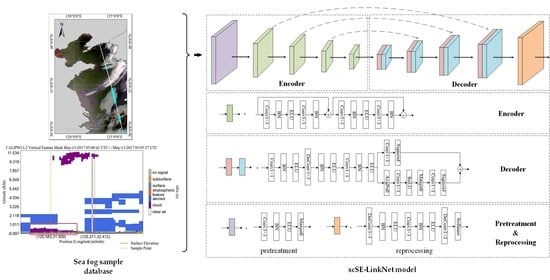
Combined with the sea fog monitor report from China’s meteorological observatory, we selected 60 MODIS images from 2016 to 2018 when sea fog events occurred near the Bohai Sea and Yellow Sea in China. Then, we used CALIOP VFM products to assist the manual interpretation of MODIS images to build a ground sample database for training the deep learning model. The ground sample set was produced from the time sequence of sea fog event occurrence from 2016 to 2018, and the time noted below are UTC time.
The main preprocessing steps of MODIS data include radiometric calibration, solar zenith angle correction, brightness temperature calculation [32], geometric correction [33], and land–ocean masking. According to previous research on the correlation analysis results of MODIS channels on sea fog characteristics [34], we selected three bands to make sea fog samples, namely a visible channel (band 1), a near infrared channel (band 17), and a longwave infrared channel (band32) with central wavelengths of 0.645, 0.905, and 12.02 μm, respectively. In order to improve the accuracy of manual interpretation samples, the CALIOP VFM product was used to assist in interpreting the features on the MODIS images. The superposition result of MODIS data and CALIOP data is shown in Figure 8. The CALIOP VFM product cannot directly judge whether there is sea fog. Referring to the work by Zhao [35] and Liu [24], we considered cloud top height of less than 1 km, cloud base close to the surface, or cloud area with no signal as the sea fog/low cloud.
Referencing the region growing algorithm [36] and the Tobler’s First Law of Geography that everything is related to everything else, but near things are more related to each other, it is believed that the CALIOP trajectory single point pixel within a certain range, such as pixels, is the same as the ground type where the CALIOP trajectory single point pixel is masked. Finally, we obtained the true label of the ground samples with two classes containing sea fog samples and other (middle/high cloud, stratus clouds, low cloud, and sea surface) samples. The size of the MODIS images were different at different times. Moreover, larger remote sensing images that need to be classified are directly input into the network, which may cause memory overflow. To make the input image size uniform, the original image and the corresponding label were randomly cropped to the same size of for subsequent model training with a total of 42,598,400 pixels, of which 6,553,140 pixels were sea fog pixels.
The MODIS band value used in this study included reflectance and brightness temperature with different numerical ranges. To avoid reducing the training accuracy due to excessive numerical differences, the sample data were standardized before inputting to the network. The specific formula is as follows:
where is the normalized result, is the value before normalization, is the expectation of , and is the variance of . After normalization, the expected value of the sample was 0 and the variance was 1.
4.2. Experimental Settings
In this study, the sample set was randomly divided into training set (520 images) and test set (130 images) in the ratio of 8:2. The training set was used to train the scSE-LinkNet model, and the test set was used to calculate various evaluation indicators and evaluate the generalization ability of the model.
In the sea fog detection field, we have access to fewer ground truth labels of sea fog, so the weights of the model cannot converge to the global optimum values, thus limiting the model performance. Data augmentation can help us generate new samples to compensate for the small training datasets [37]. Before model training, the samples in the training set were randomly flipped and rotated at any angle of 0° to 180° before each iteration.
For model optimization, instead of ReLU, we used the ELU activation function proposed by Clevert [38] as it has an exponential shape and provides a nonlinear modeling capability for the network. The mathematical expression is as follows:
where is an input feature, and is an adjustable parameter that controls the value to which an ELU saturates for negative net inputs [38].
There was a large difference in the number of samples of sea fog and other ground objects, with the number of other ground objects being the largest and sea fog being the smallest. Therefore, in this study, we used focal loss function [39] to replace the cross entropy function, which can reduce the weight of the large number of samples in training and improve the sea fog detection accuracy. The formula of the focal loss function is as follows:
where the focusing parameter smoothly adjusts the rate at which easy samples are downweighted, is the model’s estimated probability for the label , reflects the proximity between the true label and predicted category [39].
In this work, scSE-LinkNet was implemented using the open-source framework PyTorch [40]. The specific information of network training is shown in Table 2.
Considering both resources and efficiency, Adam with a learning rate of 0.001 was chosen as the optimization algorithm as it has strong robustness in the selection of super parameters. The learning rate decay factor was 0.0001, and the learning rate adjustment formula is as follows:
where is the number of training epochs, is the learning rate decay, and is the learning rate. While training the localization task, the training data batch size was set to 8, and 150 epochs were trained on the network. When the accuracy no longer improved, the training was stopped. The final model training accuracy was 96.9%.
4.3. Experimental Results
4.3.1. Performance Comparison of CNN Models
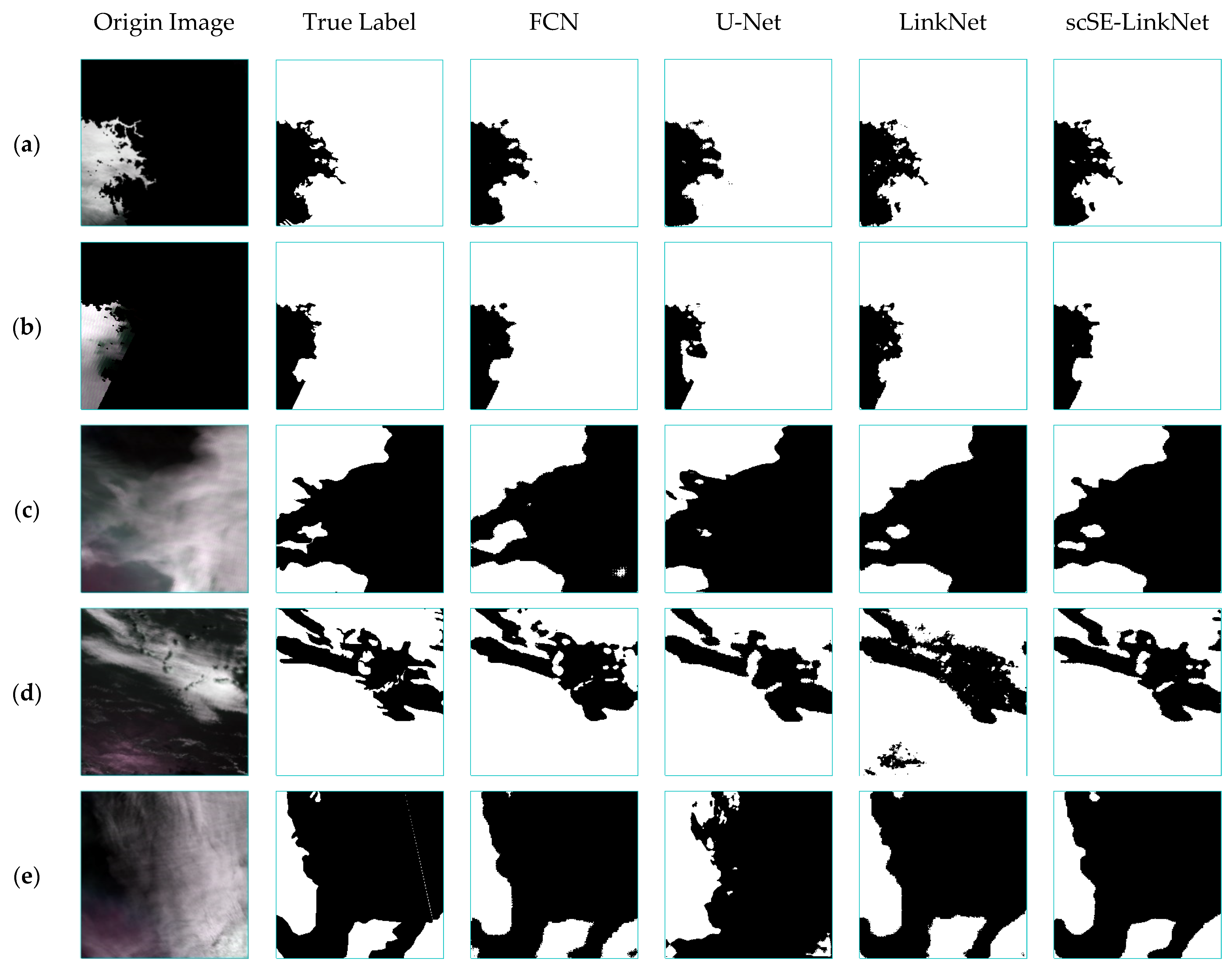
In order to show the experimental results of the scSE-LinkNet model, we used samples from the test set to obtain the sea fog detection results, which were compared with the results of conventional semantic segmentation network (FCN, U-Net, and LinkNet). The sea fog detection results are shown in Figure 9.
As shown in Figure 9a,b, compared with other models, the sea fog detection results of scSE-LinkNet could identify the edge of sea fog more accurately and could better outline the sea fog distribution area. However, there was some blurring of sea fog edge recognition with the scSE-LinkNet model, as shown in Figure 9c–e, which may be related to the feature of the sea fog sample itself. Overall, the sea fog detection result with scSE-LinkNet model was the closest to the true label, while the result with U-Net was the worst.
To further evaluate the difference in sea fog detection results, we quantitatively evaluated different algorithms on the test set. With hits, false alarms, misses and correct negatives indicated as H, F, M and C, the definitions of POD, FAR, CSI, and HSS are as follows:
We used the training set (520 images) to train different models and used the test set (130 images) to calculate the total number of fog and non-fog pixels according to the labels of the samples. Taking 130 images of the experimental data, the POD, FAR, CSI, and HSS of the sea fog detection results are shown in Table 3.
From Table 3, it is clear that scSE-LinkNet had the highest POD and CSI, and its FAR was the lowest. scSE-LinkNet had a good performance improvement compared to LinkNet and U-Net, especially the CSI, which was improved by 8.1%. Compared with the FCN method, scSE-LinkNet improved the POD and CSI by 1.50% and 5.7%, respectively. It was clear that adding the scSE module to the decoder of the LinkNet resulted in better performance. Therefore, it can be concluded that our proposed model achieved higher accuracy in the test set.
The size of the sea fog detection images obtained through the network should be the same as the input size of the training images. In this study, the input training samples were , and the sea fog detection results predicted by the model were also the same size. However, the original MODIS images were relatively large, generally pixels, which cannot directly be input into scSE-LinkNet for prediction. Therefore, before using MODIS images for sea fog detection, we needed to crop the image into a series of images with the size of and input them into the model for prediction [41]. Then, we restored the prediction results to the original image size according to the crop order to obtain the final sea fog detection results.
4.3.2. Validation with Measured Data
Considering scSE-LinkNet is among the semantic segmentation networks that use two-dimensional images, it can be difficult to achieve quantitative verification. In this study, we selected sea fog events in April 2018 to qualitatively validate the sea fog detection results with different semantic segmentation model by ICOADS data and meteorological station data. The distribution of the measured data from ICOADS and meteorological station data are shown in Figure 10.
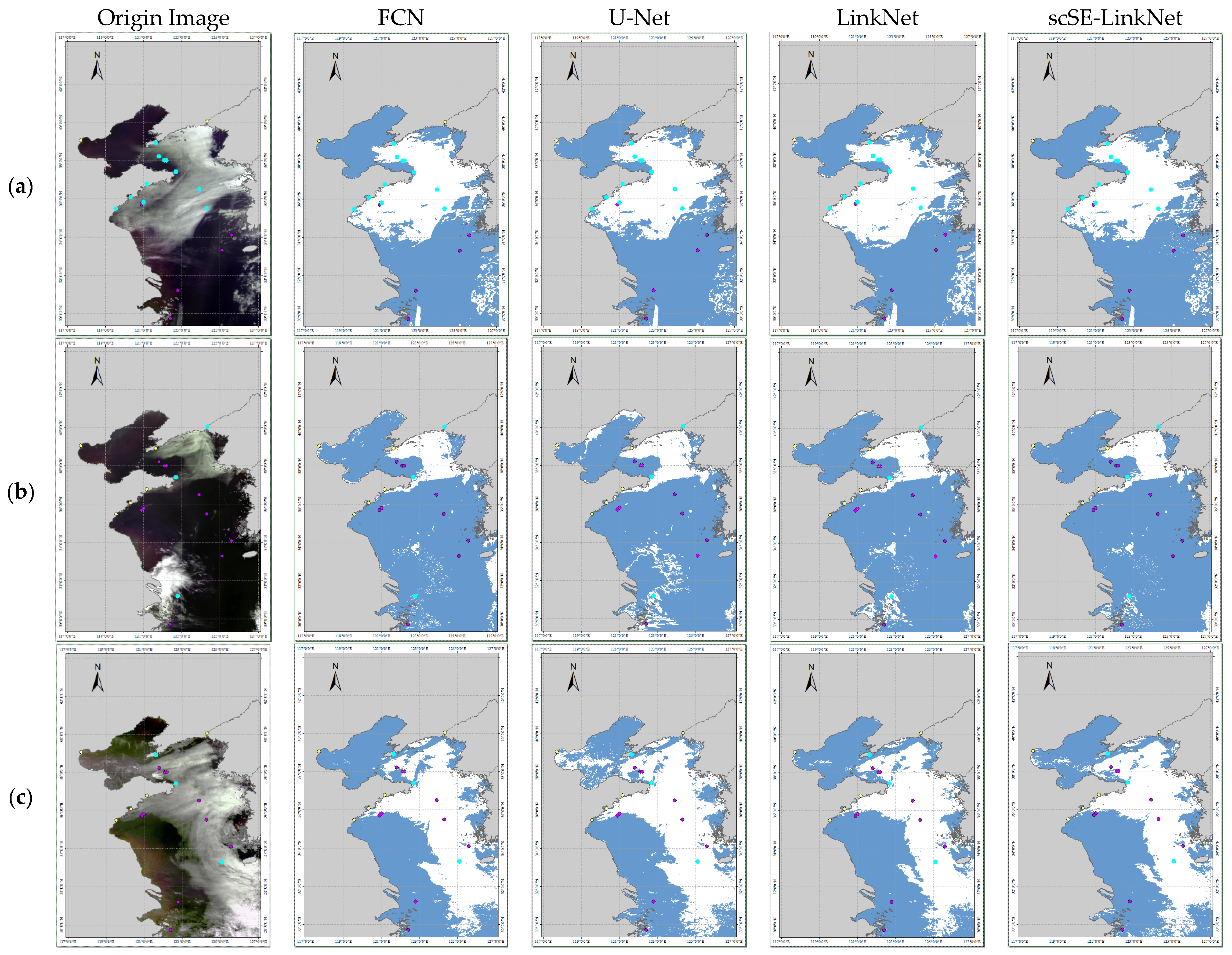
Figure 11 shows the sea fog detection results by different semantic segmentation models, which were overlaid with measured data to achieve qualitative analysis of sea fog detection results. The first column shows the number of sea fog cases on 1 April 2018 at 05:30 UTC, 2 April 2018 at 04:35 UTC, and 30 April 2018 at 05:00 UTC. The second column shows the true color RGB images. The other columns show the detection results from FCN, U-Net, LinkNet, and scSE-LinkNet. As shown in Figure 11a, the sea fog detection results from different models were consistent with the measured data. The sea fog detection results of the FCN model did not match one measured point, and the detection results from the other models were consistent with the measured data in Figure 11b. As can be seen in Figure 11c, the sea fog detection results obtained by all models were not consistent with the measured data obtained by the Dalian station. It may be that there was mist at the Dalian station that the constructed model could not identify.
4.3.3. Validation with CALIOP VFM Products
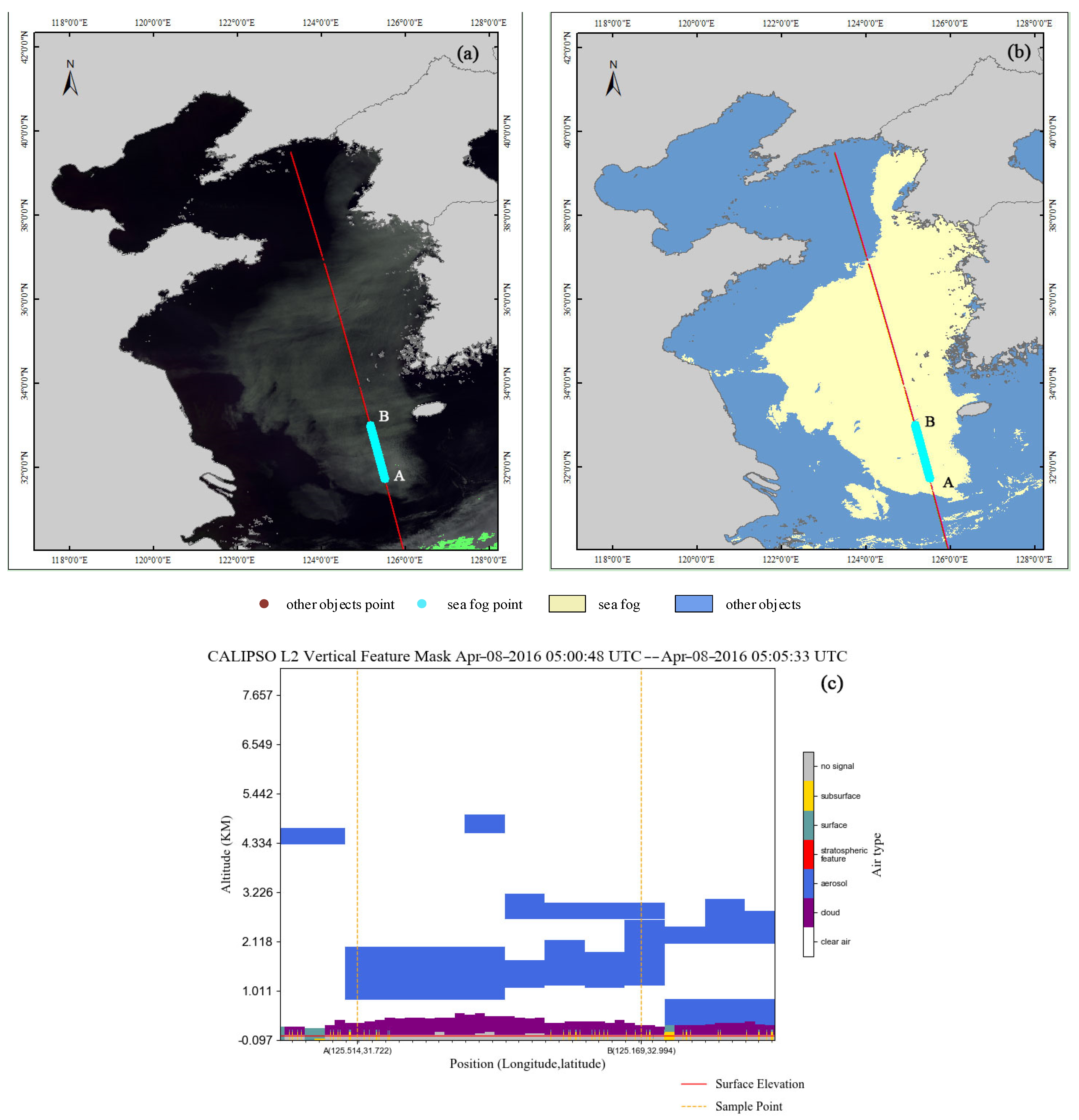
In this study, we used the CALIOP VFM product to further validate the scSE-LinkNet algorithm of sea fog detection. We selected the sea fog event at 05:00 UTC on 8 April 2016 to validate the detection result (Figure 12b). At this time, the main part of the fog area was in the middle of the Yellow Sea, north to the northeast coast of North Korea, and east to the Korean Peninsula. The red line in Figure 12a is the trajectory of the CALIOP VFM product, and the sea fog points are highlighted in blue.
As mentioned in Section 4.1, we considered cloud top height of less than 1 km, cloud base close to the surface, or cloud area with no signal as the sea fog/low cloud. Figure 12 shows the sea fog detection results and CALIOP VFM data profile at 05:00 UTC on 8 April 2016. The points in Figure 12a,b are labeled as A to B from south to north. Combined with the VFM profile (Figure 12c), it can be seen that the cloud top height in region A (125.514°N, 31.772°E) to B (125.169°N, 32.994°E) was below 1 km, and the height of the cloud base (purple parts) was similar to the surface (green parts), which is consistent with the criteria for fog. The no-signal area in gray is regarded as thicker sea fog or low cloud, and radar signal cannot penetrate them. The detection result of sea fog was consistent with the VFM profile. Judging from the sea fog detection result from scSE-LinkNet, the main part of the sea fog area was mostly the same as the true MODIS image. The sea fog pixels from A to B were fully consistent with the CALIOP trajectory, indicating that the detection result was credible to a certain extent.
5. Discussion
The scSE-LinkNet deep learning model for daytime sea fog detection proposed in this study combines scSE module with LinkNet to obtain better sea fog detection results. In the experiment, the initial problem was the sample accuracy from manual interpretation. In order to improve the accuracy of samples, we used fog monitoring reports to select the date of sea fog events and then used CALIOP VFM products to assist manual interpretation, which reduced the subjectivity of selecting samples. The second problem was choosing a suitable network with fewer training samples. The channel reduction scheme and ResNet18 pretraining parameters in scSE-LinkNet reduce the training parameters, and the scSE module in the decoder layer can learn the spectral and spatial information of the nodes, which can improve the ability of the model to extract global information. Compared to other semantic segmentation networks, our proposed model achieved the best performance for both FAR and CSI (Table 3).
In order to prove that scSE-LinkNet has the advantage of using fewer training samples, we designed a sensitive analysis. In this experiment, we set the minimum number of training set to 220 images and increased them in intervals of 50 images until the maximum number of images reached 520. Moreover, eight different training sets were used to train scSE-LinkNet. The trained models were then tested on the test set (130 images) to calculate the POD, FAR, and CSI evaluation metrics. The distribution of POD, FAR, and CSI are shown in Figure 13.
As shown in Figure 13, the value of POD and CSI tended to increase with the number of samples in the training set, and the value of FAR tended to decrease. When the number of samples was greater than 420, the CSI was stable above 0.7, with a high accuracy rate of sea fog detection. This demonstrates that scSE-LinkNet can be used for sea fog detection with fewer training samples and that a training set with a sample size above 420 can achieve better detection results.
Because 2D images were used in our model, it was difficult to calculate the evaluation index between the sea fog results and measured data. To further learn the difference between the model detection result and the measured value, we used measured data from ICOADS and meteorological station for qualitative verification. The sea fog detection results were consistent with the measured data. Then, we used CALIOP VFM products to validate a single sea fog event. The verification result was consistent with the VFM profile, thereby illustrating the accuracy of the sea fog detection result from scSE-LinkNet.
However, it should be pointed out that the recognition result of the model trained by deep learning is greatly affected by the number and accuracy of training samples. Although we tried our best to minimize the impact of subjectivity on sample production, the manual interpretation of samples would have affected the sea fog detection results. How to use other data to further improve the accuracy of manual interpretation of sea fog samples is a worthy research in the future.
6. Conclusions
In this study, a scSE-LinkNet model that utilizes MODIS images and CALIOP VFM data was used for daytime sea fog detection. First, the accuracy of manual interpretation was improved using MODIS data assisted by CALIOP VFM data, which helped improve the accuracy of model training. Then, the scSE-LinkNet model was designed, which added attention mechanism to each layer of the LinkNet decoders by considering the spectral and spatial information of the nodes. The use of spatial relationship knowledge boosted the performance and robustness of the module. In addition, the ELU activation function and focal loss function alleviated the phenomenon of sample imbalance and improved the accuracy of the model.
The sea fog detection results of scSE-LinkNet were consistent with ICOADS data, meteorological station data, and CALIOP VFM products. The POD, FAR, CSI, and HSS of the model in the test set were 0.924, 0.143, 0.800, and 0.864, respectively. Compared with other algorithms, the scSE-LinkNet model had the highest CSI and the lowest FAR, indicating that the model used in this study is feasible for daytime sea fog detection.
Author Contributions
J.W. and X.G. conceived and designed the research and performed the experiments. X.G. wrote and edited the paper. S.L., M.X. and M.Y. gave advice for the preparation and revision of the paper. S.L. and H.S. supervised the project. All authors have read and agreed to the published version of the manuscript.
Funding
This research was supported by the National Natural Science Foundation of China (Grant No. 41776182), the National Key R&D program (Grant No. 2017YFC1405600) and the Key Research and Development Program of Shandong Province (Grant No. 2019GHY112034).
Institutional Review Board Statement
Not applicable.
Informed Consent Statement
Not applicable.
Data Availability Statement
The data used in this paper are all public data sets, which can be obtained free of charge through websites and books. The data sources are detailed in Section 2.2.
Acknowledgments
We would like to thank all the people who helped and supported our research, especially Jianhua Wan, Mingming Xu, and Muhammad Yasir. And thanks to anonymous reviewers for constructive and helpful suggestions on the manuscript.
Conflicts of Interest
The authors declare no conflict of interest.
References
- Deng, J.; Bai, J.; Liu, J.; Wang, X.; Shi, H. Detection of daytime fog using MODIS multispectral data. Meteorol. Sci. Technol. 2006, 34, 188–193. [Google Scholar]
- Zhang, S.; Bao, X. The main advances in sea fog research in China. Period. Ocean Univ. China 2008, 03, 359–366. [Google Scholar]
- Mahdavi, S.; Amani, M.; Bullock, T.; Beale, S. A Probability-Based Daytime Algorithm for Sea Fog Detection Using GOES-16 Imagery. IEEE J. Sel. Topics Appl. Earth Observ. 2021, 14, 1363–1373. [Google Scholar] [CrossRef]
- Yuan, Y.; Qiu, Z.; Sun, D.; Wang, S.; Yue, X. Daytime sea fog retrieval based on GOCI data: A case study over the Yellow Sea. Opt. Express 2016, 24, 87–801. [Google Scholar] [CrossRef] [PubMed]
- Fu, G.; Guo, J.; Pendergrass, A.; Li, P. An analysis and modeling study of a sea fog event of over the Yellow and Bohai Seas. J. Ocean Univ. China 2008, 7, 27–34. [Google Scholar] [CrossRef]
- Koračin, D.; Dorman, C.E.; Lewis, J.M.; Hudson, J.G.; Wilcox, E.M.; Torregrosa, A. Marine fog: A review. Atmos. Res. 2014, 143, 142–175. [Google Scholar] [CrossRef]
- Lee, T.F.; Turk, F.J.; Richardson, K. Stratus and Fog Products Using GOES-8–9 3.9-μm Data. Weather Forecast. 1997, 12, 664–677. [Google Scholar] [CrossRef]
- Cermak, J.; Bendix, J. A novel approach to fog/low stratus detection using Meteosat 8 data. Atmos. Res. 2008, 87, 279–292. [Google Scholar] [CrossRef]
- Bendix, J.; Thies, B.; Cermak, J.; Nauß, T. Ground Fog Detection from Space Based on MODIS Daytime Data—A Feasibility Study. Weather Forecast. 2005, 20, 989–1005. [Google Scholar] [CrossRef]
- Heo, K.Y.; Min, S.Y.; Ha, K.J.; Kim, J.H. Discrimination between sea fog and low stratus using texture structure of MODIS satellite images. Korean J. Remote Sens. 2008, 24, 571–581. [Google Scholar]
- Ryu, H.S.; Hong, S. Sea Fog Detection Based on Normalized Difference Snow Index Using Advanced Himawari Imager Observations. Remote Sens. 2020, 12, 1521. [Google Scholar] [CrossRef]
- Han, J.H.; Suh, M.S.; Yu, H.Y.; Roh, N.Y. Development of Fog Detection Algorithm Using GK2A/AMI and Ground Data. Atmos. Remote Sens. 2020, 12, 3181. [Google Scholar] [CrossRef]
- Yang, J.-H.; Yoo, J.-M.; Choi, Y.-S. Advanced Dual-Satellite Method for Detection of Low Stratus and Fog near Japan at Dawn from FY-4A and Himawari-8. Remote Sens. 2021, 13, 1042. [Google Scholar] [CrossRef]
- Deng, Y.; Wang, J.; Cao, J.; Cao, C. Detection of Daytime Fog in South China Sea Using MODIS Data. J. Trop. Meteorol. 2014, 20, 386–390. [Google Scholar]
- Zhang, S.; Yi, L. A Comprehensive Dynamic Threshold Algorithm for Daytime Sea Fog Retrieval over the Chinese Adjacent Seas. Pure Appl. Geophys. 2013, 170, 1931–1944. [Google Scholar] [CrossRef]
- Wan, J.H.; Jiang, L.; Xiao, Y.F.; Sheng, H. Sea fog detection based on dynamic threshold algorithm at dawn and dusk time. In Proceedings of the International Archives of Photogrammetry, Remote Sensing and Spatial Information Sciences, Nanjing, China, 25–27 October 2019. [Google Scholar]
- Wu, X.; Li, S. Automatic sea fog detection over Chinese adjacent oceans using Terra/MODIS data. Int. J. Remote Sens. 2014, 35, 7430–7457. [Google Scholar] [CrossRef]
- Wu, D.; Lu, B.; Zhang, T.; Yan, F. A method of detecting sea fogs using CALIOP data and its application to improve MODIS-based sea fog detection. J. Quant. Spectrosc. Radiat. Transf. 2015, 153, 88–94. [Google Scholar] [CrossRef]
- Xiao, Y.; Zhang, J.; Qin, P. An Algorithm for Daytime Sea Fog Detection over the Greenland Sea Based on MODIS and CALIOP Data. J. Coast. Res. 2019, 90, 95–103. [Google Scholar] [CrossRef]
- Wan, J.; Su, J.; Liu, S.; Sheng, H. The research on the spectral characteristics of sea fog based on CALIOP and MODIS data. In Proceedings of the International Archives of the Photogrammetry, Remote Sensing and Spatial Information Sciences, Beijing, China, 7–10 May 2018. [Google Scholar]
- Shin, D.; Kim, J.H. A New Application of Unsupervised Learning to Nighttime Sea Fog Detection. Asia Pac. J. Atmos. Sci. 2018, 54, 527–544. [Google Scholar] [CrossRef] [Green Version]
- Kim, D.; Park, M.S.; Park, Y.J.; Kim, W. Geostationary Ocean Color Imager (GOCI) Marine Fog Detection in Combination with Himawari-8 Based on the Decision Tree. Remote Sens. 2020, 12, 149. [Google Scholar] [CrossRef] [Green Version]
- Drönner, J.; Korfhage, N.; Egli, S.; Mühling, M.; Thies, B.; Bendix, J.; Freisleben, B.; Seeger, B. Fast Cloud Segmentation Using Convolutional Neural Networks. Remote Sens. 2018, 10, 1782. [Google Scholar] [CrossRef] [Green Version]
- Liu, S.; Yi, L.; Zhang, S.; Xue, Y. A Study of Daytime Sea Fog Retrieval over the Yellow Sea Based on Fully Convolutional Networks. Trans. Oceanol. Limnol. 2019, 6, 13–22. [Google Scholar]
- Zhu, C.; Wan, J.; Liu, S.; Xiao, Y. Sea Fog Detection Using U-Net Deep Learning Model Based on Modis Data. In Proceedings of the 2019 10th Workshop on Hyperspectral Imaging and Signal Processing: Evolution in Remote Sensing (WHISPERS), Amsterdam, The Netherlands, 24–26 September 2019. [Google Scholar]
- Jeon, H.K.; Kim, S.; Edwin, J.; Yang, C.S. Sea Fog Identification from GOCI Images Using CNN Transfer Learning Models. Electronics 2020, 9, 311. [Google Scholar] [CrossRef]
- Koračin, D.; Dorman, C.E. Marine Fog: Challenges and Advancements in Observations, Modeling, and Forecasting, 3rd ed.; Springer: Cham, Switzerland, 2017; p. 2. [Google Scholar]
- Freeman, E.; Woodruff, S.D.; Worley, S.J.; Lubker, S.J.; Kent, E.C.; Angel, W.E.; Berry, D.I.; Brohan, P.; Eastman, R.; Gates, L.; et al. ICOADS Release 3.0: A major update to the historical marine climate record. Int. J. Climatol. 2016, 27, 2211–2232. [Google Scholar] [CrossRef] [Green Version]
- Chaurasia, A.; Culurciello, E. LinkNet: Exploiting encoder representations for efficient semantic segmentation. In Proceedings of the 2017 IEEE Visual Communications and Image Processing (VCIP), St. Petersburg, FL, USA, 10–13 December 2017. [Google Scholar]
- Hu, J.; Shen, L.; Albanie, S.; Sun, G.; Wu, E. Squeeze-and-Excitation Networks. IEEE Trans. Pattern Anal. Mach. Intell. 2020, 42, 2011–2023. [Google Scholar] [CrossRef] [Green Version]
- Roy, A.G.; Navab, N.; Wachinger, C. Concurrent spatial and channel ‘squeeze & excitation’in fully convolutional networks. In Proceedings of the Medical Image Computing and Computer Assisted Intervention (MICCAI), Granada, Spain, 16–20 September 2018. [Google Scholar]
- Meng, L.K.; Tao, L.; Li, J.Y.; Wang, C.X. A system for automatic processing of MODIS L1B data. In Proceedings of the 8th International Symposium on Spatial Accuracy Assessment in Natural Resources and Environmental Sciences, Shanghai, China, 25–27 June 2008. [Google Scholar]
- GU, L.J.; Ren, R.Z.; Wang, H.F. MODIS imagery geometric precision correction based on longitude and latitude information. J. China Univ. Posts Telecommun. 2010, 17, 73–78. [Google Scholar] [CrossRef]
- Zhang, J.; Zhang, S.; Wu, X.; Liu, Y.; Liu, J. The research on Yellow Sea sea fog based on MODIS data: Sea fog properties retrieval and spatial-temporal distribution. Period. Ocean Univ. China 2009, 39, 311–318. [Google Scholar]
- Zhao, J.; Wu, D.; Zhao, Y. A Method for Sea Fog Detection Using CALIOP Data. Period. Ocean Univ. China 2017, 47, 9–15. [Google Scholar]
- Zhu, S.; Yuille, A. Region competition: Unifying snakes, region growing, and Bayes/MDL for multiband image segmentation. IEEE Trans. Pattern Anal. Mach. Intell. 1996, 18, 884–900. [Google Scholar]
- Wang, Z.; Gao, X.; Zhang, Y. HA-Net: A Lake Water Body Extraction Network Based on Hybrid-Scale Attention and Transfer Learning. Remote Sens. 2021, 13, 4121. [Google Scholar] [CrossRef]
- Clevert, D.A.; Unterthiner, T.; Hochreiter, S. Fast and accurate deep network learning by exponential linear units (ELUs). In Proceedings of the International Conference on Learning Representations, San Juan, PR, USA, 2–4 March 2016. [Google Scholar]
- Lin, T.; Goyal, P.; Girshick, R.; He, K.; Dollár, P. Focal Loss for Dense Object Detection. IEEE Trans. Pattern Anal. Mach. Intell. 2020, 42, 318–327. [Google Scholar] [CrossRef] [PubMed] [Green Version]
- Paszke, A.; Gross, S.; Massa, F.; Lerer, A.; Bradbury, J.; Chanan, G.; Killeen, T.; Lin, Z.; Gimelshein, N.; Antiga, L.; et al. Pytorch: An imperative style, high-performance deep learning library. In Proceedings of the Advances in Neural Information Processing Systems, Vancouver, BC, Canada, 8–14 December 2019. [Google Scholar]
- Wang, Z.Q.; Zhou, Y.; Wang, S.X.; Wang, F.T.; Xu, Z.Y. House building extraction from high-resolution remote sensing images based on IEU-Net. Natl. Remote Sens. Bull. 2021, 25, 2245–2254. [Google Scholar]
Figure 1.
Geographical location of the study area.

Figure 2.
Flow chart of the sea fog detection method.

Figure 3.
LinkNet architecture: (a) the whole structure of LinkNet, (b) encoder block of LinkNet, and (c) decoder block of LinkNet. m represents input feature map; n represents output feature map.
Figure 3.
LinkNet architecture: (a) the whole structure of LinkNet, (b) encoder block of LinkNet, and (c) decoder block of LinkNet. m represents input feature map; n represents output feature map.

Figure 4.
SE module. represents any transformation of feature maps, represents the squeeze transformation, represents the excitation transformation, and represents the scale transformation.
Figure 4.
SE module. represents any transformation of feature maps, represents the squeeze transformation, represents the excitation transformation, and represents the scale transformation.

Figure 5.
The structure of scSE-LinkNet.

Figure 6.
The structure of the spatial and channel squeeze-and-excitation block (scSE). σ(∙) represents sigmoid.
Figure 6.
The structure of the spatial and channel squeeze-and-excitation block (scSE). σ(∙) represents sigmoid.

Figure 7.
Convolutional modules in decoder block. m represents input feature map; n represents output feature map.
Figure 7.
Convolutional modules in decoder block. m represents input feature map; n represents output feature map.

Figure 8.
The superimposed result of MODIS and CALIOP data. (a) True color red–green–blue (RGB) images from 13 May 2017 at 05:00 UTC; the yellow line represents the CALIOP trajectory line, and the blue points represents sea fog points. (b) CALIOP VFM data profile. The sample points in red squares in (a,b) are sea fog samples.

Figure 9.
The sea fog detection result of different deep learning model with samples from test set, (a–e) are randomly selected samples of the test set.
Figure 9.
The sea fog detection result of different deep learning model with samples from test set, (a–e) are randomly selected samples of the test set.

Figure 10.
Distribution of the measured data in April 2018. The yellow points are measured data from meteorological station, and the purple points are measured data from ICOADS.
Figure 10.
Distribution of the measured data in April 2018. The yellow points are measured data from meteorological station, and the purple points are measured data from ICOADS.

Figure 11.
The sea fog detection results with different models. The white areas represents sea fog detection results, and the blue points represent the measured data consistent with sea fog detection results during the time of sea fog occurrence. (a) 1 April 2018 at 05:30 UTC, (b) 2 April 2018 at 04:35 UTC, (c) 30 April 2018 at 05:00 UTC.

Figure 12.
The sea fog detection results and CALIOP VFM data profile at 05:00 UTC on 8 April 2016. (a) The MODIS image, (b) the verified points distribution in the sea fog detection result, (c) the VFM profile of the sea fog detection result.
Figure 12.
The sea fog detection results and CALIOP VFM data profile at 05:00 UTC on 8 April 2016. (a) The MODIS image, (b) the verified points distribution in the sea fog detection result, (c) the VFM profile of the sea fog detection result.

Figure 13.
Distribution of sea fog evaluation metrics with different sample numbers.


Table 1.
Meteorological station information along the study area.
| Station Name | Station Number | Latitude and Longitude |
|---|---|---|
| Dandong | 54497 | (40.03°N, 124.33°E) |
| Dalian | 54662 | (38.91°N, 121.64°E) |
| Weihai | 54776 | (37.40°N, 122.70°E) |
| Yantai | 54863 | (36.78°N, 121.18°E) |
| Qingdao | 54857 | (36.07°N, 120.33°E) |
| Rizhao | 54945 | (35.47°N, 119.56°E) |
| Tanggu | 54623 | (39.05°N, 117.72°E) |
Table 2.
The specific information of network training.
| Platform | Version | CPU | GPU |
|---|---|---|---|
| Windows 10 | Python 3.7 PyTorch 1.2.0 | AMD Ryzen 5 3600 CPU (3.80 GHz) | NVIDIA 2060 SUPER GPU (8 GB RAM) |
Table 3.
The evaluation index of different algorithms.
| CNN Models | POD | FAR | CSI | HSS |
|---|---|---|---|---|
| FCN | 0.909 | 0.197 | 0.743 | 0.819 |
| U-Net | 0.880 | 0.202 | 0.719 | 0.799 |
| LinkNet | 0.916 | 0.171 | 0.771 | 0.841 |
| scSE-LinkNet | 0.924 | 0.143 | 0.800 | 0.864 |
Publisher’s Note: MDPI stays neutral with regard to jurisdictional claims in published maps and institutional affiliations. |
© 2021 by the authors. Licensee MDPI, Basel, Switzerland. This article is an open access article distributed under the terms and conditions of the Creative Commons Attribution (CC BY) license (https://creativecommons.org/licenses/by/4.0/).
Share and Cite
MDPI and ACS Style
Guo, X.; Wan, J.; Liu, S.; Xu, M.; Sheng, H.; Yasir, M. A scSE-LinkNet Deep Learning Model for Daytime Sea Fog Detection. Remote Sens. 2021, 13, 5163. https://0-doi-org.brum.beds.ac.uk/10.3390/rs13245163
AMA Style
Guo X, Wan J, Liu S, Xu M, Sheng H, Yasir M. A scSE-LinkNet Deep Learning Model for Daytime Sea Fog Detection. Remote Sensing. 2021; 13(24):5163. https://0-doi-org.brum.beds.ac.uk/10.3390/rs13245163
Chicago/Turabian StyleGuo, Xiaofei, Jianhua Wan, Shanwei Liu, Mingming Xu, Hui Sheng, and Muhammad Yasir. 2021. "A scSE-LinkNet Deep Learning Model for Daytime Sea Fog Detection" Remote Sensing 13, no. 24: 5163. https://0-doi-org.brum.beds.ac.uk/10.3390/rs13245163
Note that from the first issue of 2016, this journal uses article numbers instead of page numbers. See further details here.