
LIME-Based Data Selection Method for SAR Images Generation Using GAN


1
School of Electronic Engineering, Xidian University, Xi’an 710071, China
2
School of Electronic Information and Artificial Intelligence, Shaanxi University of Science and Technology, Xi’an 710021, China
*
Author to whom correspondence should be addressed.
Remote Sens. 2022, 14(1), 204; https://0-doi-org.brum.beds.ac.uk/10.3390/rs14010204
Submission received: 23 November 2021
/
Revised: 27 December 2021
/
Accepted: 30 December 2021
/
Published: 3 January 2022
(This article belongs to the Special Issue Explainable Deep Neural Networks for Remote Sensing Image Understanding)
Abstract
:Deep learning has obtained remarkable achievements in computer vision, especially image and video processing. However, in synthetic aperture radar (SAR) image recognition, the application of DNNs is usually restricted due to data insufficiency. To augment datasets, generative adversarial networks (GANs) are usually used to generate numerous photo-realistic SAR images. Although there are many pixel-level metrics to measure GAN’s performance from the quality of generated SAR images, there are few measurements to evaluate whether the generated SAR images include the most representative features of the target. In this case, the classifier probably categorizes a SAR image into the corresponding class based on “wrong” criterion, i.e., “Clever Hans”. In this paper, local interpretable model-agnostic explanation (LIME) is innovatively utilized to evaluate whether a generated SAR image possessed the most representative features of a specific kind of target. Firstly, LIME is used to visualize positive contributions of the input SAR image to the correct prediction of the classifier. Subsequently, these representative SAR images can be selected handily by evaluating how much the positive contribution region matches the target. Experimental results demonstrate that the proposed method can ally “Clever Hans” phenomenon greatly caused by the spurious relationship between generated SAR images and the corresponding classes.
1. Introduction
Synthetic aperture radar (SAR) can realize full-time observation and obtain high-resolution SAR images without being restricted by weather and light, thus it is widely applied in both civil and military fields [1]. Target recognition is generally considered as the most challenging process in SAR image interpretation because of the complex procedures in the feature extraction and classification [2]. With the development of high-performance computers, deep learning has gradually become popular in computer vision and natural language processing [3]. Deep learning methods autonomously learn the inner relationship between massive labeled data and the corresponding categories. However, SAR images are extremely limited and difficult to collect in large quantities. Worse, even if we can collect enough raw data, manually labeling them is time-consuming and labor-intensive. In this case, SAR image simulation draws increasing attention. Traditional SAR image simulation methods are mainly based on ray-tracing and rasterization theories [4,5,6]. Unfortunately, the generated simulation images through traditional methods are quite different from the real SAR images. Worse, these methods are quite time-consuming. This limitation can be alleviated with the emergence of various generative adversarial networks (GANs). Ian J. Goodfellow et al. proposed GAN in 2014 [7]. GANs can generate spurious samples by mimicking the data distribution of real samples. However, it is usually difficult to train a stable GAN due to various issues such as mode collapse, training instability, and ambiguity in model evaluation. Refs. [8,9] proposed deep convolutional generative adversarial network (DCGAN) and Wasserstein generative adversarial network (WGAN) to alleviate the mode collapse from the aspects of network structure and loss function, respectively. Note that the aforementioned GANs can only generate SAR images without labels, thus it is still difficult to use these data directly in SAR image recognition. To provide labeled images, Mirza and Osindero [10] proposed the conditional generative adversarial network (CGAN) to control the properties of generated images. The label of generated images is corresponding to the conditional information input to the model, such as category information, semantic information, etc. Cao et al. [11] proposed a label-directed generative adversarial network (LDGAN) to alleviate the issue of data insufficiency of data-driven based SAR target recognition methods. In the multi-constraint generative adversarial network (MCGAN) designed by Du et al. [12], the input of generator is features learned by an encoder rather than random noise, which can effectively generate high-quality labeled SAR images. Ref. [13] presented a hierarchical GAN to gradually generate high-resolution SAR images through a multi-stage model.
Although there are numerous novel GANs that can improve the quality of generated SAR images, Clever Hans, a serious problem on networks’ interpretation, is seldom considered. Clever Hans [14] is a famous example of observer expectation effects. Hans was a horse that conquered the audience with the extraordinary ability of mathematical calculations. In fact, Hans did not carry out a real reasoning process but just relied on unconscious cues from the trainers and the observers, such as facial expressions, postures, etc., to give the correct answer. The “Clever Hans” phenomenon often appears in the field of deep learning [15], i.e., although the trained classifiers can achieve high accuracy, they do not really learn the features or strategies that match people’s cognition, but learn the spurious connection between the trained samples and their labels. In this case, the “Clever Hans”-type decision strategy will probably fail to provide reliable and stable classification, which may be disqualifying or even unacceptable for some low-risk tolerance scenarios, such as medical, finance, automatic driving, military, etc. Therefore, it is necessary and significant to understand the internal mechanism of DNN to prevent it from “Clever Hans”-type decision making.
Multiple methods were proposed to visualize the internal mechanism of deep neural networks (DNNs). The methods can be divided into four categories: Propagation-based method, Class activation mapping (CAM) method, Perturbation-based method, and model-agnostic method. Propagation-based methods visualize the correlation between input and output by decomposing the result of the output layer and propagating it to the input space layer by layer according to the designed propagation rules [16,17]. CAM methods visualize the area of interest of the model by providing a highlighted region to reflect the networks’ interest in a specific class by weighted summation of feature maps [18,19,20,21,22]. Perturbation-based methods observe the change of the output by masking, deleting, or blurring different regions of the input, thereby, determining the impact of the corresponding region on the output [23,24]. Model-agnostic methods are currently state-of-the-art interpretation methods, e.g., local interpretable model-agnostic explanation (LIME) [25], Shapley Additive exPlanation (SHAP) [26], etc. They can give a relatively uniform interpretation for various types of machine learning models. LIME is a practical and effective method for describing and verifying the behavior of non-linear deep learning algorithms. It helps to evaluate whether the trained model has learned the features or strategies that people expect. Few of the SAR image generation methods based on deep learning consider the influence of the “Clever Hans” phenomenon. In this case, the labeled images are likely to be generated according to the spurious relationship between the real samples and the corresponding classes. To avoid this, we proposed a data selection method based on LIME to alleviate “Clever Hans” phenomenon. In our proposed method, the visualization results of the classifier obtained by LIME are utilized as the detectors of “Clever Hans” phenomenon to select the training data of GAN from the MSTAR dataset. LIME is adopted to visualize the classifier since LIME has the following advantages compared with other methods: (1) LIME is a model-agnostic method with good versatility and less computational burden compared with perturbation-based method; (2) There are usually numerous scattered speckles in the heatmap generated by Propagation-based method, which will not appear in the result of LIME method; (3) CAM method visualizes only positive contributions to the result, while LIME can mark both the positive and negative contributions to the result, respectively. We conduct experiments on the moving and stationary target acquisition and recognition (MSTAR) dataset to verify the effectiveness of our proposed method. Note that, our aim is to explore the effectiveness of LIME method in alleviating the “Clever Hans” phenomenon in DNNs, but not to obtain a GAN with superior performance by optimizing the architecture and the loss function of the GAN. Despite this, the GAN employed in this study still generates images of high quality.
The follow-up contents of this article are arranged as follows: Section 2 reviews the algorithm of C-DCGAN and LIME. Section 3 describes our method in detail. Section 4 presents some experimental results from different perspectives. Section 5 discusses the experimental results and the future research direction. Section 6 gives the conclusions.
2. Materials and Methods
2.1. Conditional Deep Convolutional GAN
The GAN is composed of a generator G and a discriminator D. It alternately optimizes G and D by playing the two-player min–max game with the value function until they reach the Nash equilibrium point [7]. Assume that represents the distribution of the real data x, represents the prior distribution of random noise vector z. The optimization goal of the GAN can be written as:
The generation process of the original GAN lacks operability and semantics due to the randomness of the input data, thus it is impossible to generate samples with specified characteristics. In response to this shortcoming, Mirza and Sindero [10] added conditional information on the basis of basic GAN, and proposed CGAN. The algorithm introduces the condition information y, such as category information, semantic information, etc., in both the generator and the discriminator. The conditional information y is spliced with the hidden variable z and the input image x as the input of G and D, respectively. The objective function of the training would be as:
Multi-layer perceptron (MLP) has difficulty capturing the local correlation in the image, therefore GANs with the MLP structure usually cannot achieve ideal generation effects on some complex image datasets. To solve this problem, Alec Radford et al. proposed DCGAN [8]. It only retains the fully connected layer in the input layer of the G and the output layer of the D, and uses step convolution and deconvolution to replace the pooling operation to implement the down-sampling and up-sampling operations, respectively. The output layer of the G uses the Tanh function as the activation function, and the other layers use the ReLU function. The D uses LeakyReLU as the activation function in all layers. In addition, it introduces the batch normalization layer to stabilize the training of the model.
In this paper, we utilize CGAN with the deep convolution structure (C-DCGAN), and choose category information as the conditional information. The detailed architecture of C-DCGAN is presented in Figure 1.
2.2. Local Interpretable Mode-Agnostic Explanation
LIME was proposed by Ribeiro et al. [25] to explain the prediction of arbitrary classifiers. The overall idea of LIME is training an interpretable model to approximate the explained deep model in the local range. The explained deep model is represented as f. We define an interpretable model , G represents the family of all possible simple models, such as linear regression models, logistic regression models, decision trees, etc. Mathematically, the explanation of the input sample x obtained by the local surrogate model can be expressed as:
The model complexity is kept low to ensure the interpretability of g, e.g., a shallow depth for decision trees or a small number of non-zero weights for linear models. In practice, we usually directly constrain the complexity, e.g., by determining the number of non-zero coefficients of the linear regression model. Therefore, LIME only optimizes the loss part . measures how close the explanation obtained by g is to the prediction of the explained deep model f. Mathematically, we can use the following formula to measure the difference between the predictions of the two models:
where z, are the perturbed instances with dimension corresponding to the input layer of f and g, respectively. The similarity kernel defines the locality of the interpreted sample x. It is believed that the closer the distance to the original sample x, the greater the weight, i.e., the greater the impact. defined on distance measure function D with width can be expressed as:
For images, D is usually the L2 distance.
Specifically, LIME trains the local surrogate model according to the following steps: Firstly, the image instance x is segmented into superpixels by any standard algorithm, e.g., Turbopixel [27], Quick-shift [28], SLIC [29], etc. Secondly, the perturbed instances can be obtained by turning superpixels off or on. A superpixel can be turned off by replacing each pixel in it with a user-defined color, such as black. Thirdly, we recover the perturbed instances to the original input space and obtain z as the new input of f. The predictions of z are the corresponding labels of the perturbed instances. Subsequently, and form the nearest neighbor dataset of the input sample. Finally, g is trained on the dataset Z.
In conclusion, LIME uses the perturbed instances obtained in the neighborhood around instance x to train the interpretable model to achieve the purpose of always in the local range. Consequently, the explained deep model can be replaced locally by the trained interpretable model. The flowchart of LIME is described in Figure 2.
3. Our Method
The SAR images generated by GANs according to the spurious connection between the real SAR images and the corresponding labels can not be applied to SAR target recognition due to lack of authenticity and reliability. To this end, we proposed a LIME-based data selection method to improve the quality of generated images by preventing the classifier from making “Clever Hans”-type decision. Our proposed method consists of the following five steps: (1) CNN training; (2) CNN visualization; (3) Data selection; (4) GAN training; and (5) GAN evaluation. We can select the data based on the distribution of the positive contribution delineated by LIME. The detailed processes can be described as follows:
- A CNN is trained on the MSTAR dataset. All the SAR images are converted to pseudo RGB images by repeatedly copying the monochromatic image in three channels. The input size of the SAR image is ;
- The LIME is adopted to provide the positive contribution to the CNN’s classification result of each SAR image;
- The original SAR images are selected according to the distribution of the positive contribution. The SAR images with the positive contribution in the background are discarded; The SAR images with the positive contribution coincident with targets are selected to form a new dataset;
- Two C-DCGANs are trained on the MSTAR dataset and the selected dataset, respectively, to generate two labeled SAR image datasets;
- Evaluate the two C-DCGANs based on different metrics. The evaluation results are presented in Section 4.3.
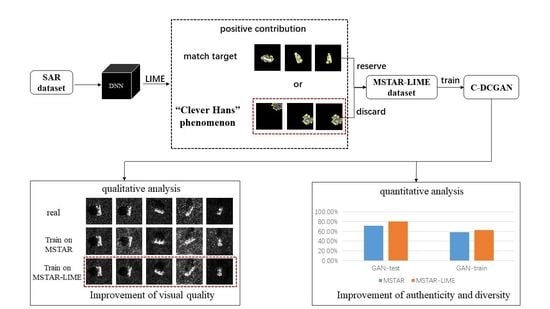
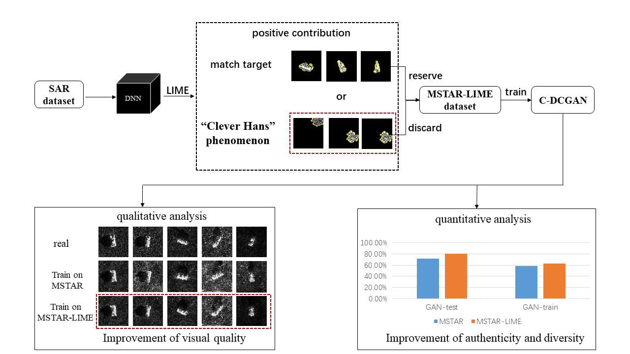
The flowchart of our proposed method is presented in Figure 3.
4. Experimental Results
In this article, the MSTAR database is employed to evaluate the performance of our method. MSTAR is a dataset composed of ten classes of real measured SAR images of ground stationary vehicles. CNN is used as the classifier in our experiments. The architecture of CNN to be visualized is presented in Figure 4. Stochastic gradient descent (SGD) was adopted as the optimizer, , . Indeed, CNN with a more exquisite structure may perform better in SAR image classification task, but the complex structure may be obstacle for interpretation, which mismatch our propose. Therefore, a lightweight CNN with an approximate accuracy of 97% is adopted as the classifier.
4.1. LIME Versus CAM Methods
In this section, experiments are conducted on MSTAR to compare the performance of LIME with Grad-CAM and Score-CAM. CAM methods generate heatmap by performing a weighted summation of the feature maps in the last convolutional layer, which can be defined as:
where is the weight of corresponding to the target class c, is the coordinate of the pixel in the feature map. The CAM methods can be divided into gradient-based and gradient-free methods according to the calculating method of .
Selvaraju et al. [18] proposed a gradient-based method: Grad-CAM. Grad-CAM uses the average channel gradient obtained in backpropagation process as the weight, which is formalized as:
where Z is the number of the pixels in the kth feature map, is the model’s prediction score of the target class c when the original image X is sent to the classification model.
Wang et al. [22] proposed a gradient-free method: Score-CAM. Score-CAM removes the dependence on the gradient, and uses the increase in confidence (CIC) of the feature map to calculate the weights. Specifically, each feature map in the last convolutional layer is upsampled and multiplied with the input image. The difference between the classification model’s prediction of the masked image and the prediction of the baseline image is used to represent the weight, defined as:
where represents the upsampling operation, is the base image set to 0.
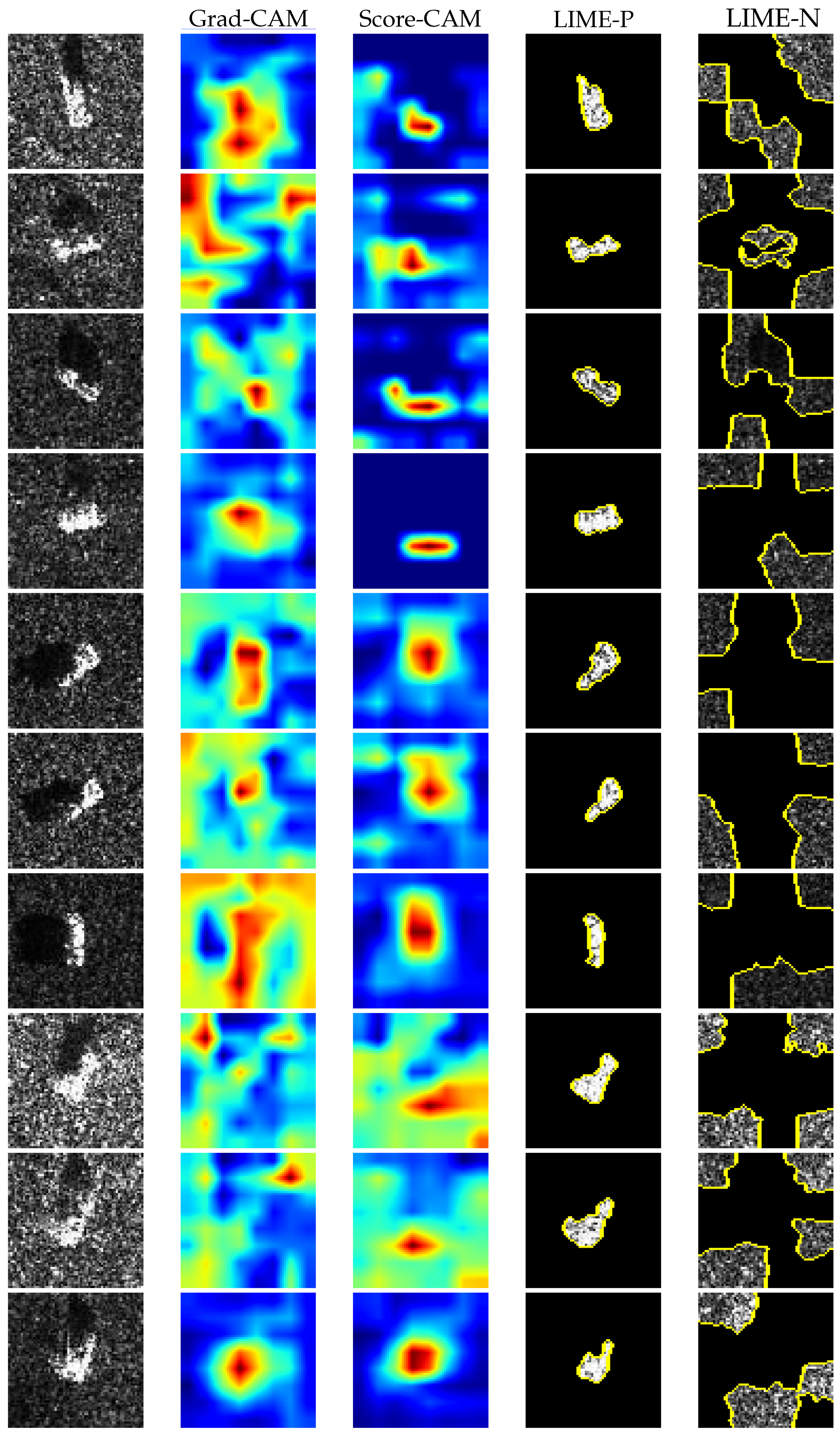
The comparison of Grad-CAM, Score-CAM and LIME is shown in Figure 5. The visualization results of CAM methods are heatmaps with the colormap set to . “LIME-P” and “LIME-N” represent the positive and negative contributions of the LIME result, respectively. It is evident that the performance of LIME is significantly better than the performance of CAM methods. CAM methods highlight areas that only contribute positively to the classifier’s decision. Conversely, LIME can reflect both positive and negative contributions to the classifier’s decision. In addition, the highlighted area in the heatmaps generated by CAM methods excessively covers the target or even deviates from the target. This is mainly caused by the process of upsampling the feature map to the size of the input image. In contrast, LIME method can delineate a region that precisely covers the target. Therefore, we can clearly observe the “Clever Hans” phenomenon in the classification task by using LIME method.
4.2. “Clever Hans” Phenomenon in SAR Image Classification Task
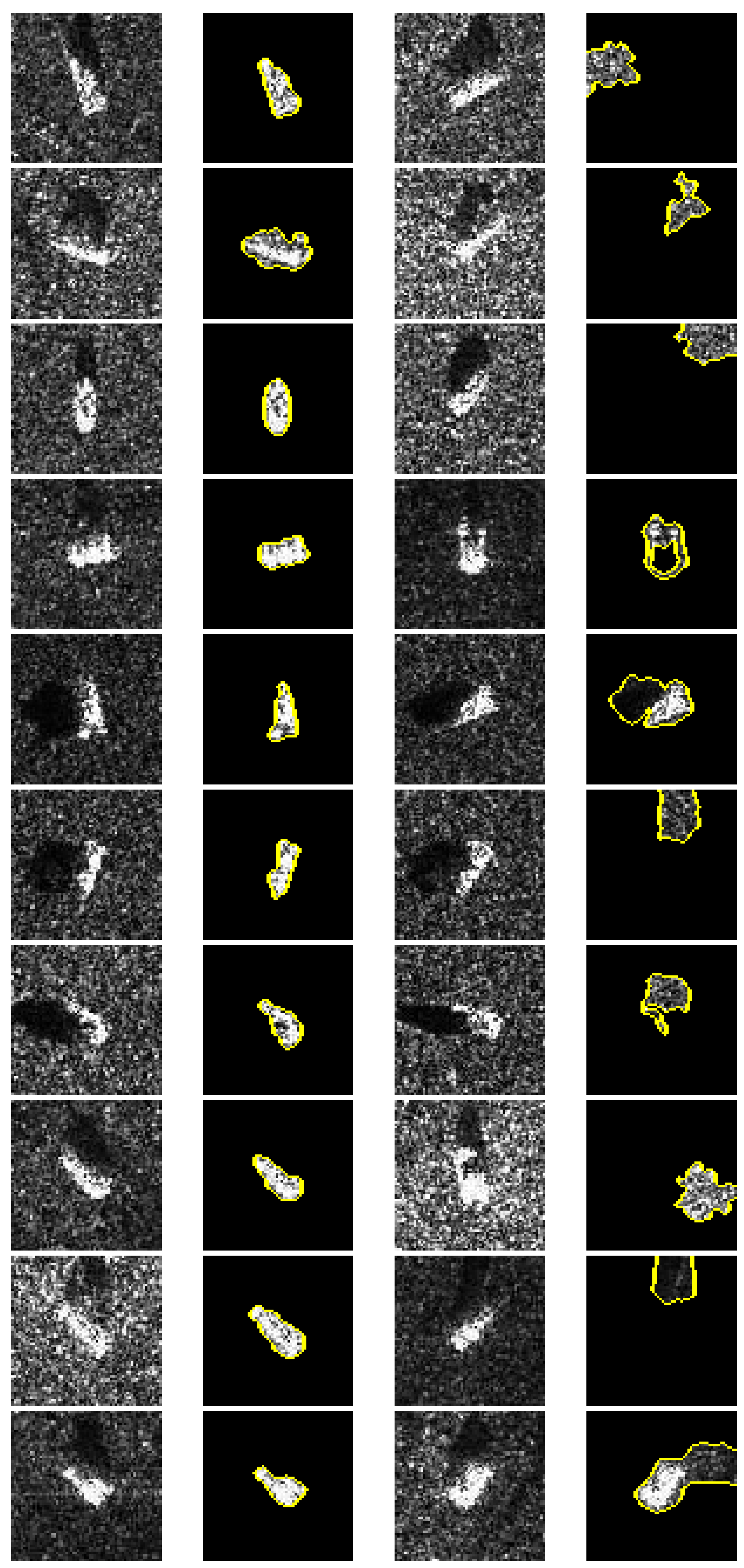
In this experiment, LIME is utilized on MSTAR dataset to observe the “Clever Hans” phenomenon in the CNN. Figure 6 presents two types of the distribution of the positive contribution, according to which we can assess whether the CNN actually reliably solves the problem we set for it. The first case is that the positive contribution is the target, as shown in the second column. It demonstrates that the CNN makes classification decisions through the difference of SAR target. This decision strategy embodied by the CNN is indeed valid and generalizable. The other case is that the positive contribution is the scattered speckles in the background, as shown in the fourth column. It indicates that the CNN implements “Clever Hans”-type decision strategy to make classification, that is, the CNN likely learns the “wrong” feature, such as the speckles around the target. The CNN that relies on “Clever Hans”-type decision strategy will probably make wrong decisions in the real scenarios where the spurious connection is not existing. Therefore, we discard this type of images to ensure that the CNN indeed learns the effective ability of correct classification.
In this experiment, we first conduct LIME on MSTAR dataset to visualize the positive contribution to the CNN’s classification result in each SAR image. Afterwards, we select the SAR images in which the positive contribution coincides with the target. The change in the number of images before and after selection is shown in Table 1, where “MSTAR-LIME” represents the result after selection. After selection, the number of images belonging to , , and is almost one-tenth of the number of the other classes. Particularly, we discard these three classes of images to avoid the problem of unbalanced sample distribution in the training of the C-DCGAN in Section 4.3.
4.3. Quality Analysis of Generated Images
In this section, we first train two C-DCGANs on the MSTAR dataset and MSTAR-LIME dataset, respectively. Then, we evaluate the visual quality, independence, authenticity, and diversity of the images generated by C-DCGANs based on different metrics, respectively.
4.3.1. Visual Quality
In this part, the generated images are subjectively evaluated through human vision. The comparison of the visual quality of two types of generated images and real images is shown in Figure 7. Compared with the images generated by C-DCGAN trained on the MSTAR dataset, the images generated by C-DCGAN trained on the MSTAR-LIME dataset have clearer contour features, more obvious scattering features, and finer texture. It indicates that the process of data selection can improve the quality of generated images.
4.3.2. Independence Analysis
In this experiment, mutual information (MI) value is employed to measure the independence between the generated images and the corresponding real images. MI value is a measure of the degree of interdependence between random variables. This experiment calculates the average of the MI values of 100 images as the final results. The comparison results of the two types of generated images and the real images are shown in Table 2. The smaller the interdependence between two images, the smaller their MI value, i.e., the independence between the two images is more obvious. It is evident from Table 2 that the MI values of the images generated by the C-DCGAN trained on the MSTAR-LIME dataset are significantly smaller than the MI values of the images generated by the C-DCGAN trained on the MSTAR dataset. In other words, the images generated by our method are more independent of the real image than the images generated by C-DCGAN without data selection. Therefore, it is more reasonable to apply the images generated by our method to the SAR target recognition task.
4.3.3. Authenticity
GAN-test [30], a measure based on the classification task, was proposed to evaluate the authenticity of images generated by GAN. GAN-test score is obtained by training the classification neural network with the real sample, and then calculating the accuracy on the validation set composed of the generated data. In this experiment, we employ the CNN presented in Figure 4 to conduct the image classification task for GAN-test measure. The GAN-test score of the two C-DCGANs is shown in Table 3. It is apparent from Table 3 that C-DCGAN trained on data selected through the LIME method can generate images that are more close to the real samples. That is because the selection process reduces the spurious relationship between the generated images and the corresponding labels.
4.3.4. Diversity
In this experiment, the GAN-train score is employed to evaluate the diversity of the generated images. GAN-train score [30] is calculated by using the generated samples to train the classifier, and then testing the classifier on the real samples. The GAN-train score is higher, the generated images are more diverse. The CNN presented in Figure 4 is utilized to conduct the image classification task for GAN-train measure. The result of GAN-train is shown in Table 4. According to Table 4, the performance of GAN-train of our proposed method is better than the generation method without data selection. Therefore, our method can generate more diverse images than the generation method without data selection.
5. Discussion
In our study, we provide qualitative and quantitative analysis to prove the effectiveness of the proposed method. In qualitative analysis, firstly the comparison of visualization results of LIME and CAM methods demonstrates that LIME can reflect the contributions to the decision comprehensively and clearly. Secondly, we provide an intuitive comparison of generated images to subjectively prove the improvement of the quality of generated images. In quantitative analysis, MI value, GAN-test score, and GAN-train score are calculated to prove the improvement of independence, authenticity, and diversity of images generated by our method.
Next, we will discuss our method from the following three aspects: (1) How does LIME perform in comparison to CAM-based approaches? LIME aims at detecting positive and negative contribution pixels, while the CAM methods aim at providing the positive contribution region by highlighting the related area. The highlighted area in the heatmaps generated by CAM methods designed for optical images usually excessively covers the target or even deviates from the target since that SAR images have low resolution and contain many interference spots. In contrast, LIME method can accurately demarcate the target area. Therefore, the “Clever Hans” phenomenon can be clearly observed in the visualization results of LIME. This is the reason why we select the dataset according to the result of LIME. (2) What are the limitations or failure modes of the technique? The limitation of this method is mainly the manual process of data selection. It is difficult to perform more detailed processing due to small extra-class differences and low resolution of SAR images. It probably would be better to use the cases in which the CNN showed “Clever Hans” decisions to guide the GAN’s training instead of discarding them entirely. However, this study aims to improve the quality of GANs by alleviating the “Clever Hans” phenomenon in DNNs instead of proposing a complicated and detailed data selection method. Therefore, the samples in which the CNN implements “Clever Hans”-type decision strategy are discarded entirely. (3) What other strategies except for data selection could be employed based on LIME (e.g., active learning), etc.? In our method, we use the result of LIME to guide the selection of SAR images. In addition, we can carry out some feature engineering work based on the result of LIME, such as removing some misleading features to focus on the generation of SAR target [21]. At a deeper level, the result of LIME can guide us to select the best model [12], i.e., we can create a model that automatically uses the visualization results to guide the training of networks. The above two research directions based on LIME will be our future research direction.
6. Conclusions
In this paper, a data selection method based on LIME is proposed to improve the quality of images generated by C-DCGAN under the “Clever Hans” phenomenon. We conduct a series of experiments on the benchmark dataset (MSTAR) to verify the validity and improvement of the method. First, the comparison with other visualization methods indicates that LIME can provide more clear visual results in network visualization based on SAR images. Second, the method converts the “Clever Hans” phenomenon in classification task into the visualization results obtained by LIME. As an innovative application, it not only explains the internal mechanism of the neural network to a certain extent but provides a basis for data selection. Finally, the experimental results based on visual quality, dependence, authenticity, and diversity verify that the GAN trained on the selected dataset can generate images with higher quality. In summary, the proposed method prevents the classifier from making decisions that depend on the “Clever Hans”-type decision strategy, thereby improving the quality and practicability of the generated images. Our proposed method also provides a new idea combined with network visualization to solve the issue of insufficient training samples in the SAR automatic target recognition task.
Author Contributions
Conceptualization, M.Z. and B.Z.; methodology, M.Z., B.Z. and L.D.; software, M.Z. and L.D.; validation, M.Z., B.Z. and L.D.; formal analysis, T.L. and Z.F.; investigation, M.Z., B.Z. and L.D.; resources, T.L., Z.F. and J.F.; data curation, J.F.; writing—original draft preparation, L.D. and Z.F.; writing—review and editing, M.Z. and B.Z.; visualization, M.Z. and B.Z.; supervision, M.Z., B.Z. and T.L.; project administration, M.Z. and B.Z.; funding acquisition, M.Z. and B.Z. All authors have read and agreed to the published version of the manuscript.
Funding
This research was funded by Science and technology project of Xianyang city, grant number: 2021ZDZX-GY-0001; the Fundamental Research Funds for the Central Universities, grant number: JB210206 and JC2111.
Institutional Review Board Statement
Not applicable.
Informed Consent Statement
Not applicable.
Data Availability Statement
In this paper, MSTAR dataset is employed for experimental verification. The MSTAR dataset is a representative dataset for testing and evaluation of current SAR target recognition methods. The dataset contains SAR images of ten classes of vehicle targets at various pitch angles, namely: 2S1, BRDM_2, BTR_60, D7, SN_132, SN_9563, SN_C71, T62, ZIL131, and ZSU_23_4. The SAR images are acquired by X-band airborne radar with a resolution of m. Readers can get the dataset from the author by email ([email protected]).
Acknowledgments
I would like to acknowledge my teammate for their wonderful collaboration and patient support. I also thank all the reviewers and editors for their great help and useful suggestions.
Conflicts of Interest
The authors declare no conflict of interest.
References
- Kong, L.; Xu, X. A MIMO-SAR Tomography Algorithm Based on Fully-Polarimetric Data. Sensors 2019, 19, 4839. [Google Scholar] [CrossRef] [Green Version]
- Lin, M.; Chen, S.; Lu, F.; Xing, M.; Wei, J. Realizing Target Detection in SAR Images Based on Multiscale Superpixel Fusion. Sensors 2021, 21, 1643. [Google Scholar] [CrossRef] [PubMed]
- Mohsenzadegan, K.; Tavakkoli, V.; Kyamakya, K. A Deep-Learning Based Visual Sensing Concept for a Robust Classification of Document Images under Real-World Hard Conditions. Sensors 2021, 21, 6763. [Google Scholar] [CrossRef] [PubMed]
- Ding, B.; Wen, G.; Huang, X.; Ma, C.; Yang, X. Data augmentation by multilevel reconstruction using attributed scattering center for SAR target recognition. IEEE Geosci. Remote Sens. Lett. 2017, 14, 979–983. [Google Scholar] [CrossRef]
- Franceschetti, G.; Guida, R.; Iodice, A.; Riccio, D.; Ruello, G. Efficient simulation of hybrid stripmap/spotlight SAR raw signals from extended scenes. IEEE Trans. Geosci. Remote Sens. 2004, 42, 2385–2396. [Google Scholar] [CrossRef]
- Martino, G.; Lodice, A.; Natale, A.; Riccio, D. Time-Domain and Monostatic-like Frequency-Domain Methods for Bistatic SAR Simulation. Sensors 2021, 21, 5012. [Google Scholar] [CrossRef] [PubMed]
- Goodfellow, I.; Pouget-Abadie, J.; Mirza, M.; Xu, B.; Warde-Farley, D.; Ozair, S.; Courville, A.; Bengio, Y. Generative Adversarial Nets. In Proceedings of the 27th International Conference on Neural Information Processing Systems, Cambridge, MA, USA, 8–13 December 2014; pp. 2672–2680. [Google Scholar]
- Radford, A.; Metz, L.; Chintala, S. Unsupervised Represention Learning with Deep Convolutional Generative Adversarial Networks. arXiv 2015, arXiv:1511.06434. [Google Scholar]
- Arjovsky, M.; Chintala, S.; Bottou, L. Wasserstein GAN. In Proceedings of the 34th International Conference on Machine Learning, Sydney, Australia, 6–11 August 2017; Volume 70, pp. 214–223. [Google Scholar]
- Shaham, U.; Yamada, Y.; Negahban, S. Conditional Generative Adversarial Nets. arXiv 2014, arXiv:1411.1784. [Google Scholar]
- Cao, C.; Cao, Z.; Cui, Z. LDGAN: A Synthetic Aperture Radar Image Generation Method for Automatic Target Recognition. IEEE Trans. Geosci. Remote Sens. 2019, 99, 1–14. [Google Scholar] [CrossRef]
- Du, S.; Hong, J.; Wang, Y.; Qi, Y. A High-Quality Multicategory SAR Images Generation Method With Multiconstraint GAN for ATR. IEEE Geosci. Remote Sens. Lett. 2021, 99, 1–5. [Google Scholar] [CrossRef]
- Huang, H.; Zhang, F.; Zhou, Y.; Yin, Q.; Hu, W. High Resolution SAR Image Synthesis with Hierarchical Generative Adversarial Networks. In Proceedings of the IGARSS 2019–2019 IEEE International Geoscience and Remote Sensing Symposium, Yokohama, Japan, 28 July–2 August 2019; pp. 2782–2785. [Google Scholar]
- Pfungst, O.; Stumpf, C.; Rahn, C.; Angell, J. Clever Hans: Contribution to experimental animal and human psychology. Philos. Psychol. Sci. Methods 1911, 8, 663–666. [Google Scholar]
- Lapuschkin, S.; Wäldchen, S.; Binder, A.; Montavon, G.; Samek, W.; Müller, K. Unmasking Clever Hans predictors and assessing what machines really learn. Nat. Commun. 2019, 10, 1. [Google Scholar] [CrossRef] [PubMed] [Green Version]
- Bach, S.; Binder, A.; Montavon, G.; Klauschen, F.; Müller, K.R.; Samek, W. On Pixel-Wise Explanations for Non-Linear Classifier Decisions by Layer-Wise Relevance Propagation. PLoS ONE 2014, 10, e0130140. [Google Scholar] [CrossRef] [PubMed] [Green Version]
- Montavon, G.; Lapuschkin, S.; Binder, A.; Samek, K.; Müller, K. Explaining NonLinear Classification Decisions with Deep Taylor Decomposition. Pattern Recognit. 2016, 65, 211–222. [Google Scholar] [CrossRef]
- Ramprasaath, R.S.; Michael, C.; Abhishek, D. Grad-CAM: Visual Explanations from Deep Networks via Gradient-based Localization. In Proceedings of the 2017 IEEE International Conference on Computer Vision (ICCV), Venice, Italy, 22–29 October 2017; pp. 618–626. [Google Scholar]
- Fu, H.; Hu, Q.; Dong, X.; Guo, Y.; Gao, Y.; Li, B. Axiom-based Grad-CAM: Towards Accurate Visualization and Explanation of CNNs. In Proceedings of the 2020 31th British Machine Vision Conference (BMVC), Manchester, UK, 7–10 September 2020. [Google Scholar]
- Saurabh, D.; Harish, G.R. Ablation-CAM: Visual Explanations for Deep Convolutional Network via Gradient-free Localization. In Proceedings of the 2020 IEEE Winter Conference on Applications of Computer Vision (WACV), Snowmass, CO, USA, 1–5 March 2020. [Google Scholar]
- Feng, Z.; Zhu, M.; Stanković, L.; Ji, H. Self-Matching CAM: A Novel Accurate Visual Explanation of CNNs for SAR Image Interpretation. Remote Sens. 2021, 13, 1772. [Google Scholar] [CrossRef]
- Wang, H.F.; Wang, Z.F.; Du, M.N. Methods for Interpreting and Understanding Deep Neural Networks. In Proceedings of the 2020 IEEE/CVF Conference on Computer Vision and Pattern Recognition Workshops (CVPRW), Seattle, WA, USA, 14–19 June 2020. [Google Scholar]
- Fong, R.; Vedaldi, A. Interpretable Explanations of Black Boxes by Meaningful Perturbation. In Proceedings of the 2017 IEEE International Conference on Computer Vision (ICCV), Venice, Italy, 22–29 October 2017; pp. 3429–3437. [Google Scholar]
- Agarwal, C.; Schonfeld, D.; Nguyen, A. Removing input features via a generative model to explain their attributions to classifier’s decisions. arXiv 2019, arXiv:1910.04256. [Google Scholar]
- Ribeiro, M.; Singh, S.; Guestrin, C. “Why Should I Trust You?”: Explaining the Predictions of Any Classifier. In Proceedings of the 22nd ACM SIGKDD International Conference on Knowledge Discovery and Data Mining, San Francisco, CA, USA, 13–17 August 2016; pp. 1135–1144. [Google Scholar]
- Lundberg, S.; Lee, S. A unified approach to interpreting model predictions. In Proceedings of the 31st International Conference on Neural Information Processing Systems, Long Beach, CA, USA, 4–9 December 2017; pp. 4768–4777. [Google Scholar]
- Levinshtein, A.; Stere, A.; Kutulakos, K.N.; Fleet, D.J.; Dickinson, S.J.; Siddiqi, K. TurboPixels: Fast Superpixels Using Geometric Flows. IEEE Trans. Pattern Anal. Mach. Intell. 2009, 31, 2290–2297. [Google Scholar] [CrossRef] [Green Version]
- Salem, M.; Ibrahim, A.F.; Ali, H.A. Automatic quick-shift method for color image segmentation. In Proceedings of the 8th International Conference on Computer Engineering & Systems (ICCES), Cairo, Egypt, 26–28 November 2013; pp. 245–251. [Google Scholar]
- Zhang, L.; Han, C.; Cheng, Y. Improved SLIC superpixel generation algorithm and its application in polarimetric SAR images classification. In Proceedings of the IEEE International Geoscience and Remote Sensing Symposium (IGARSS), Fort Worth, TX, USA, 23–28 July 2017; pp. 4578–4581. [Google Scholar]
- Shmelkon, K.; Schmid, C.; Alahari, K. How good is my GAN? In Proceedings of the European Conference on Computer Vision (ECCV), Munich, Germany, 8–14 September 2018; pp. 213–229. [Google Scholar]
Figure 1.
The architecture of C-DCGAN.

Figure 2.
The flowchart of LIME method.

Figure 3.
The flowchart of our method.

Figure 4.
The architecture of CNN.

Figure 5.
Comparison of Grad-CAM, Score-CAM, and LIME. The first column is the SAR images of ten classes: 2S1, BRDM_2, BTR_60, D7, SN_132, SN_9563, SN_C71, T62, ZIL131, ZSU_23_4. The second, third columns are corresponding heatmaps generated by Grad-CAM, Score-CAM, respectively. The fourth, fifth columns are the positive and negative contributions obtained by LIME, respectively.

Figure 6.
Revealing “Clever Hans” phenomenon of the CNN using LIME. The first and third columns are SAR images of ten classes: 2S1, BRDM_2, BTR_60, D7, SN_132, SN_9563, SN_C71, T62, ZIL131, ZSU_23_4. The second and fourth columns are corresponding results of LIME method.
Figure 6.
Revealing “Clever Hans” phenomenon of the CNN using LIME. The first and third columns are SAR images of ten classes: 2S1, BRDM_2, BTR_60, D7, SN_132, SN_9563, SN_C71, T62, ZIL131, ZSU_23_4. The second and fourth columns are corresponding results of LIME method.

Figure 7.
Comparison of visual quality of generated images and real SAR images. The first row is real SAR images of seven classes: 2S1, D7, SN_132, SN_9563, T62, ZIL131, ZSU_23_4. The second row is SAR images of the corresponding category generated by the C-DCGAN trained on the MSTAR dataset. The third row is SAR images of the corresponding category generated by the C-DCGAN trained on the MSTAR-LIME dataset.


Table 1.
Selection Result of LIME.
| 2S1 | BRDM_2 | BTR_60 | D7 | SN_132 | SN_9563 | SN_C71 | T62 | ZIL131 | ZSU_23_4 | |
|---|---|---|---|---|---|---|---|---|---|---|
| MSTAR | 573 | 572 | 452 | 573 | 428 | 486 | 427 | 572 | 573 | 573 |
| MSTAR-LIME | 520 | - | - | 567 | 425 | 393 | - | 568 | 487 | 567 |
Table 2.
MI Value.
| Before Selection | After Selection | |
|---|---|---|
| 2S1 | 1.96 | 1.78 |
| D7 | 1.41 | 1.39 |
| SN_132 | 1.37 | 1.15 |
| SN_9563 | 1.74 | 1.41 |
| T62 | 1.41 | 1.09 |
| ZIL131 | 1.31 | 1.10 |
| ZSU_23_4 | 1.53 | 1.41 |
Table 3.
GAN-test score.
| Before Selection | After Selection |
|---|---|
| 71.67% | 80.62% |
Table 4.
GAN-train score.
| Before Selection | After Selection |
|---|---|
| 58.73% | 62.56% |
Publisher’s Note: MDPI stays neutral with regard to jurisdictional claims in published maps and institutional affiliations. |
© 2022 by the authors. Licensee MDPI, Basel, Switzerland. This article is an open access article distributed under the terms and conditions of the Creative Commons Attribution (CC BY) license (https://creativecommons.org/licenses/by/4.0/).
Share and Cite
MDPI and ACS Style
Zhu, M.; Zang, B.; Ding, L.; Lei, T.; Feng, Z.; Fan, J. LIME-Based Data Selection Method for SAR Images Generation Using GAN. Remote Sens. 2022, 14, 204. https://0-doi-org.brum.beds.ac.uk/10.3390/rs14010204
AMA Style
Zhu M, Zang B, Ding L, Lei T, Feng Z, Fan J. LIME-Based Data Selection Method for SAR Images Generation Using GAN. Remote Sensing. 2022; 14(1):204. https://0-doi-org.brum.beds.ac.uk/10.3390/rs14010204
Chicago/Turabian StyleZhu, Mingzhe, Bo Zang, Linlin Ding, Tao Lei, Zhenpeng Feng, and Jingyuan Fan. 2022. "LIME-Based Data Selection Method for SAR Images Generation Using GAN" Remote Sensing 14, no. 1: 204. https://0-doi-org.brum.beds.ac.uk/10.3390/rs14010204
Note that from the first issue of 2016, this journal uses article numbers instead of page numbers. See further details here.