
A Four-Step Method for Estimating Suspended Particle Size Based on In Situ Comprehensive Observations in the Pearl River Estuary in China


Abstract
:1. Introduction
2. Materials and Methods
2.1. Study Area and Fieldwork
2.2. PSD Acquisition
2.3. Optical Property Measurements
2.4. Sentinel-2 A/B MSI Image
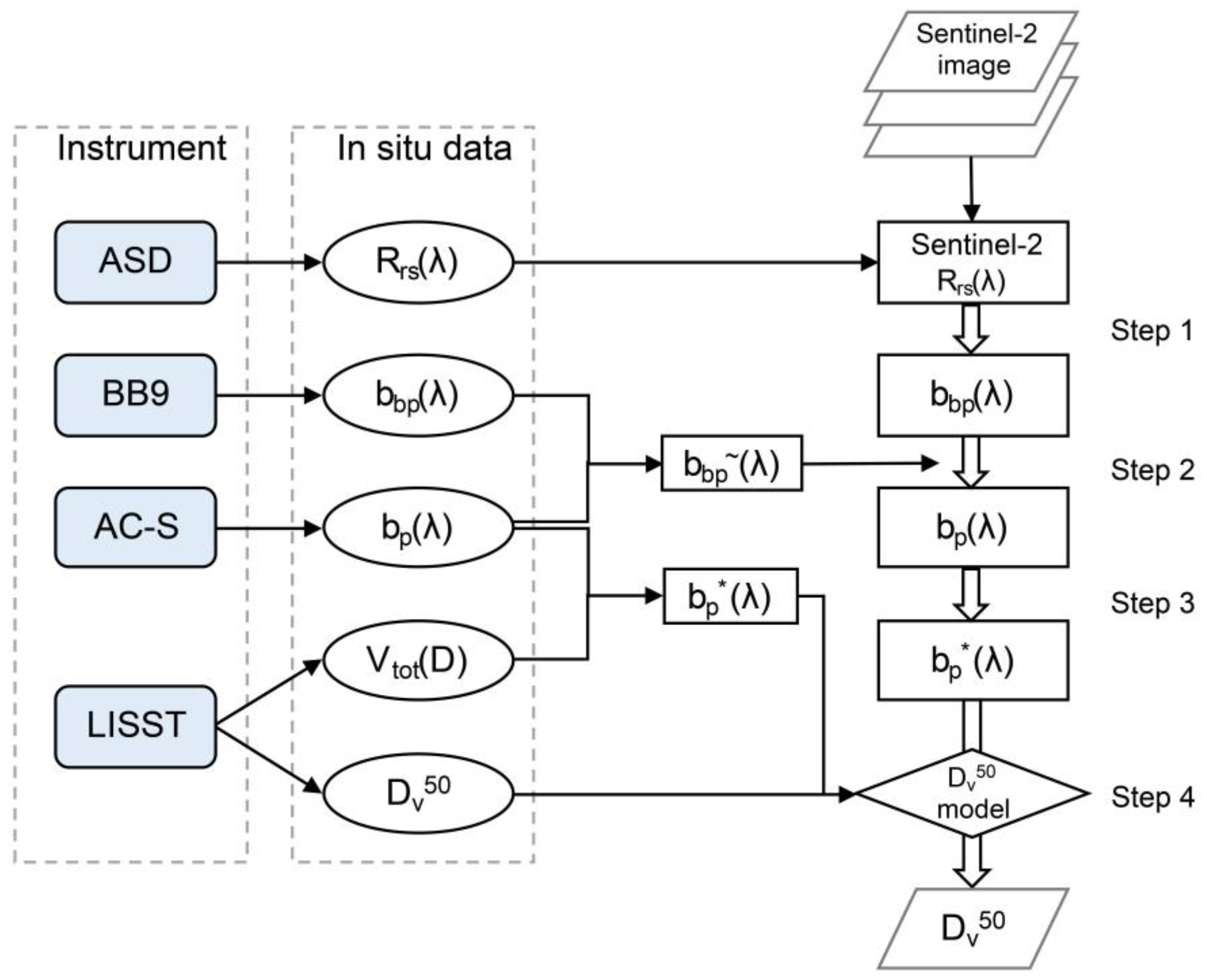
2.5. Dv50 Retrieval
2.5.1. Step 1
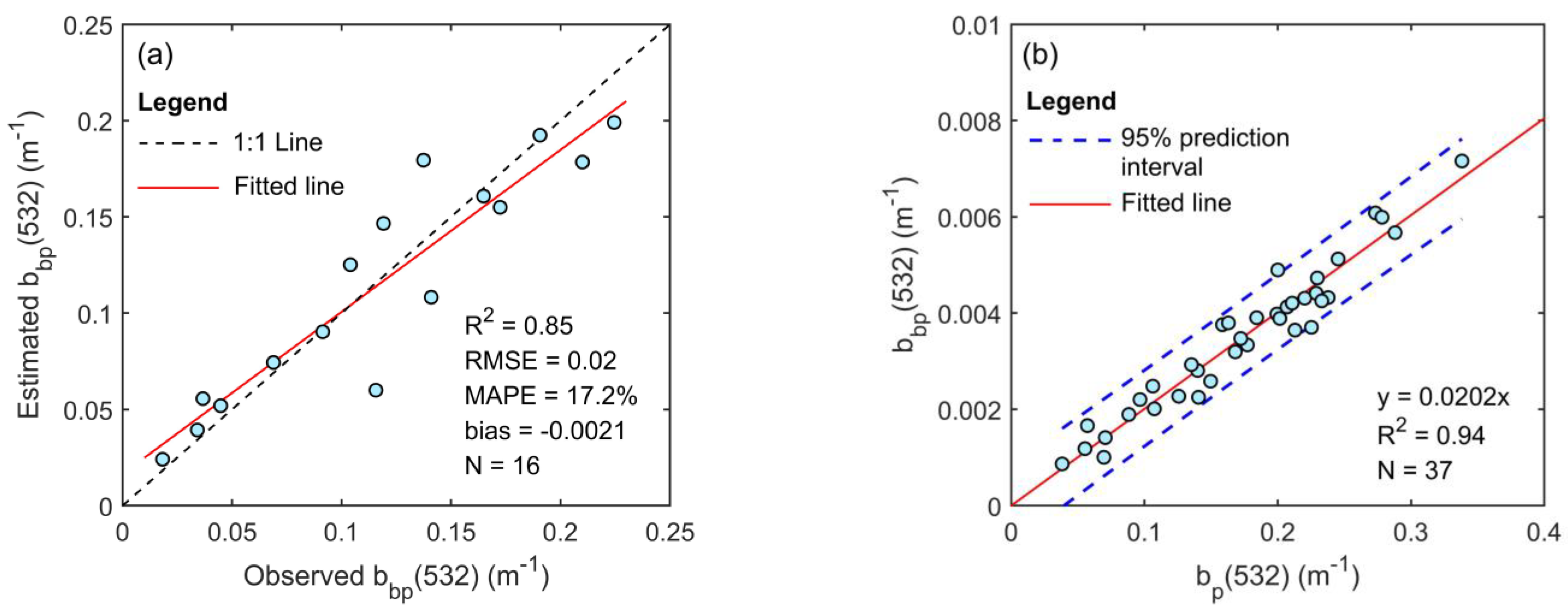
2.5.2. Step 2
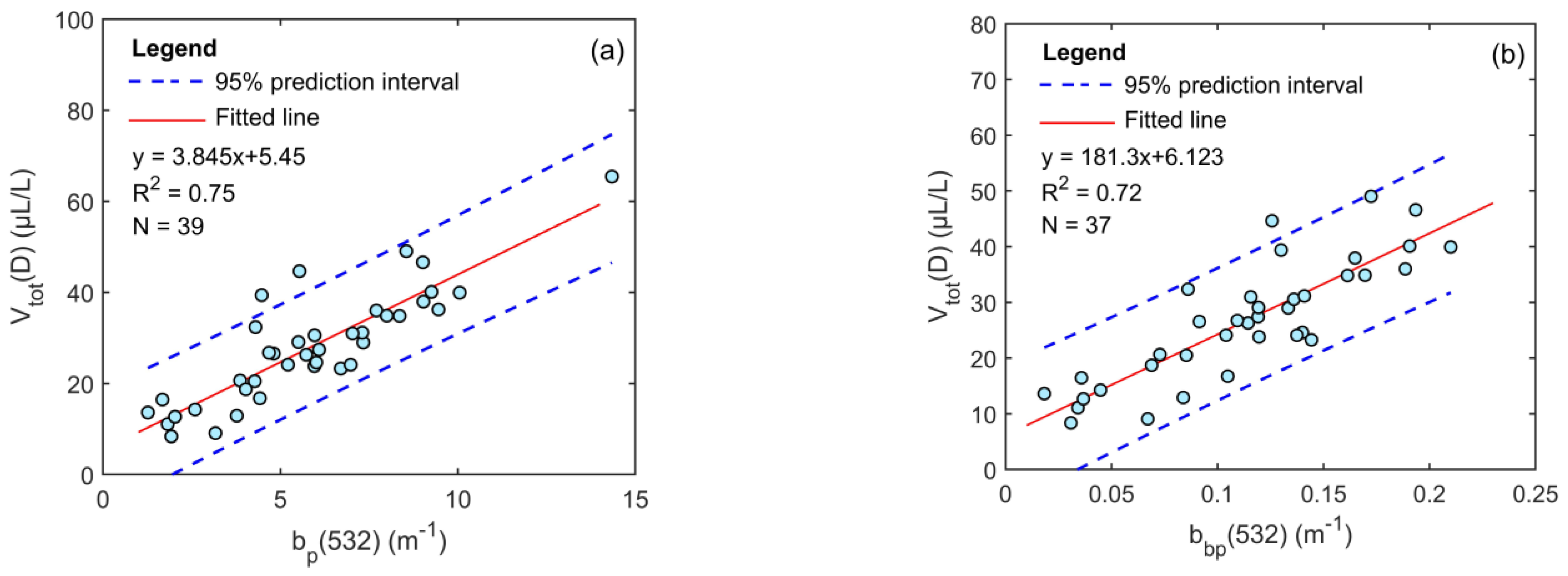
2.5.3. Step 3
2.5.4. Step 4
2.6. Accuracy Assessment
3. Results
3.1. Optical Properties and PSD
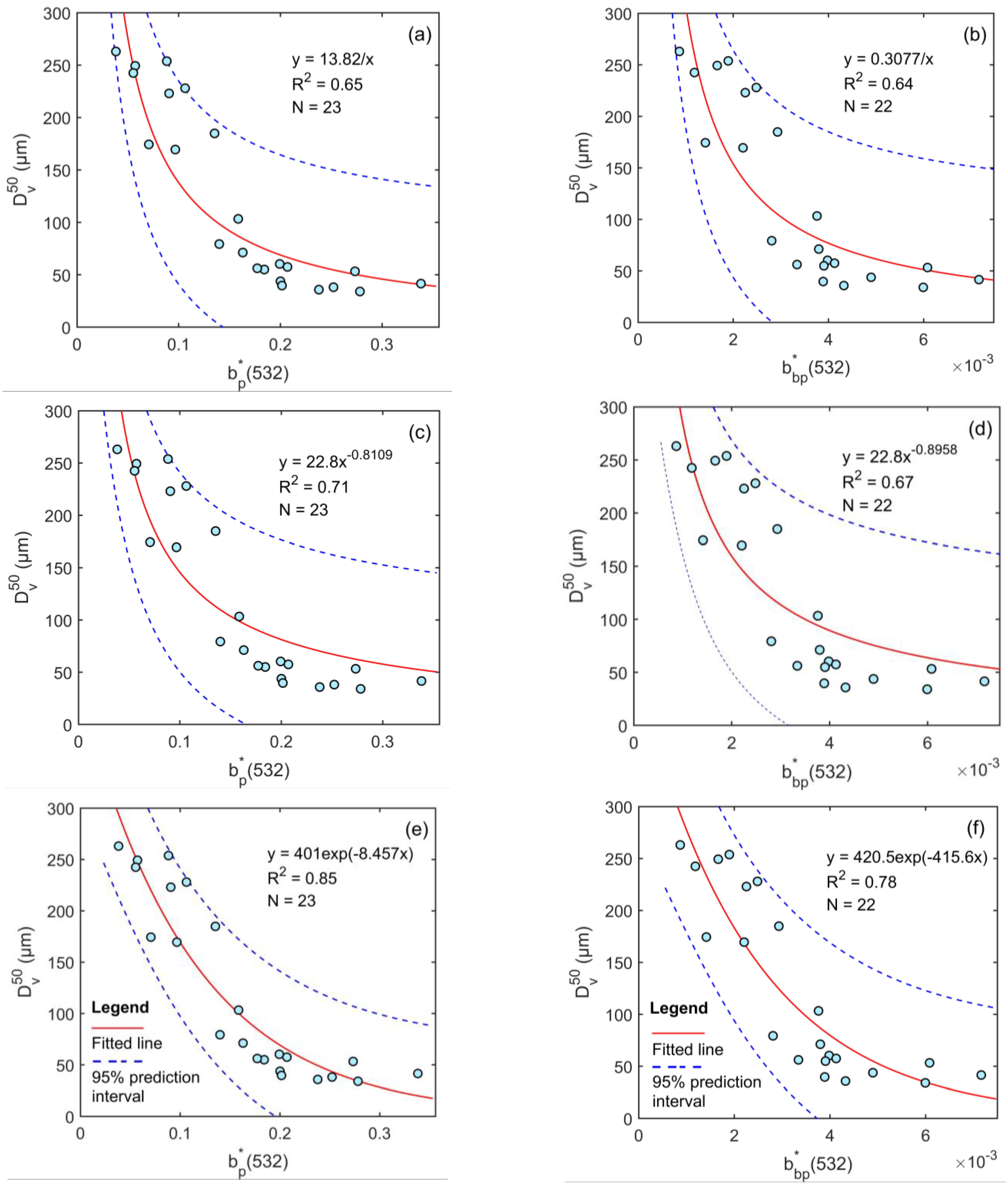
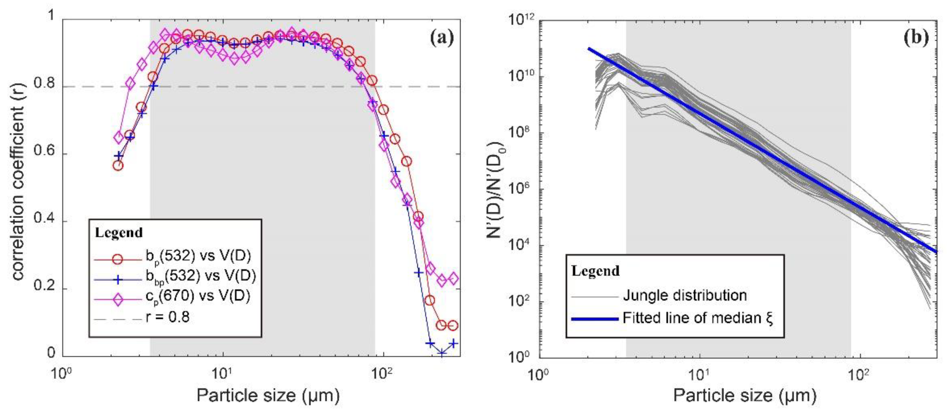
3.2. Dv50 Model Development
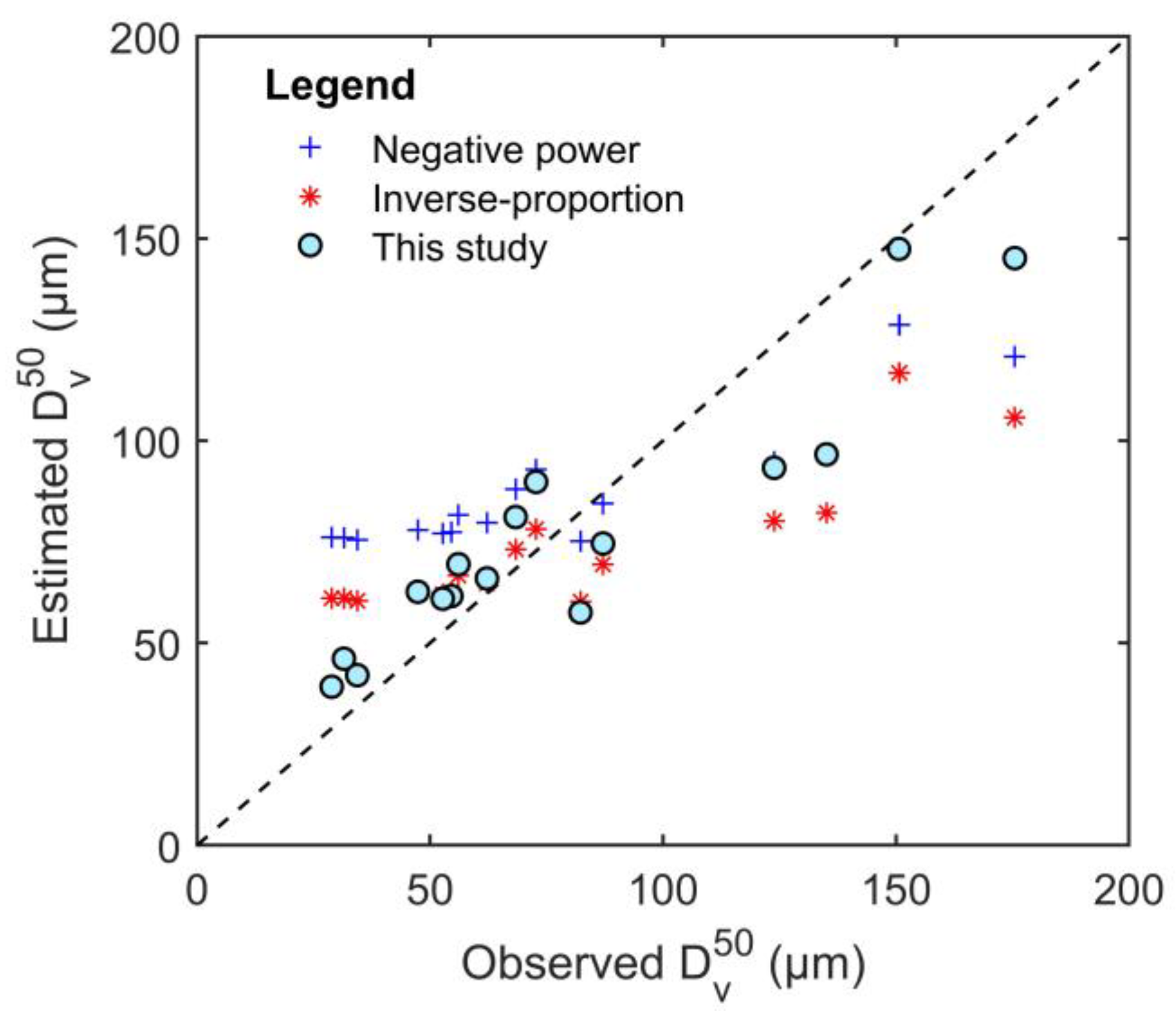
3.3. Dv50 Model Validation and Application
4. Discussion
4.1. Robustness of the Dv50 Model
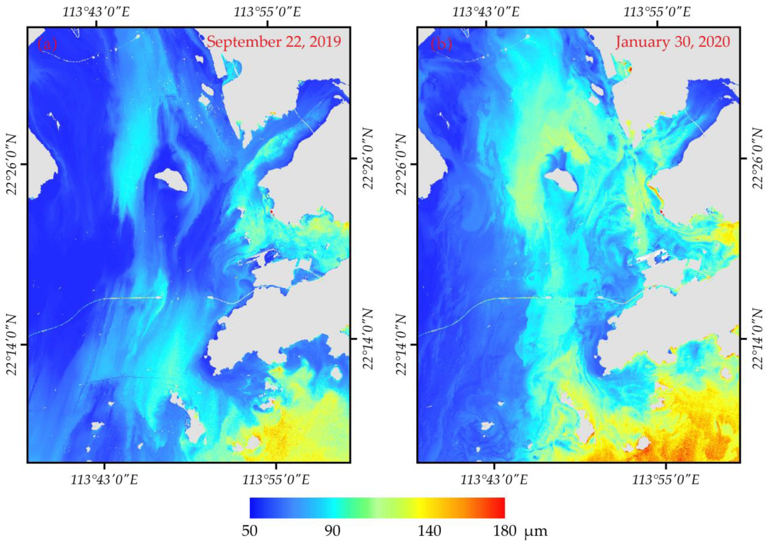
4.2. Applicability to Sentinel-2 MSI Data
5. Conclusions
Author Contributions
Funding
Institutional Review Board Statement
Informed Consent Statement
Acknowledgments
Conflicts of Interest
Abbreviations
| Variables or Abbreviations | Description |
| a | Absorption coefficient |
| aw | Absorption coefficient of pure water |
| bb | Backscattering coefficient |
| bbp | Backscattering coefficient of the particle |
| bbp~ | Backscattering ratio of the particle |
| bbw | Backscattering of pure water |
| bbp* | Volume-specific backscattering coefficient of the particle |
| bp | Scattering coefficient of the particle |
| bp* | Volume-specific scattering coefficient of the particle |
| c | Attenuation coefficient |
| CDOM | Colored dissolved organic matter |
| Chl-a | Chlorophyll-a |
| DA | Mean diameter weighted by the area |
| Dv50 | Median particle diameter |
| IOPs | Inherent optical properties |
| Lw | Radiance of the water’s surface |
| Lp | Radiance of the reference panel |
| Lsky | Radiance of the sky |
| N(D) | Particle number concentration |
| PRE | Pearl River estuary |
| PSD | Particle size distribution |
| Qbe | Scattering efficiency |
| Rrs | Remote sensing reflectance just above the water’s surface |
| rrs | Remote sensing reflectance just beneath the water’s surface |
| SRF | Spectral response function |
| TSM | Total suspended mater |
| u | Ratio of backscattering and summation of absorption and backscattering |
| V(D) | Particle volume concentration |
| Vtot(D) | Total volume concentration of the particle |
| Y | Slope of the backscattering coefficient |
| ξ | PSD slope |
| ρ | Air–water reflectance |
| ρa | Apparent density |
| ρp | Diffuse reflectance of the reference panel |
References
- Xi, H.; Larouche, P.; Tang, S.; Michel, C. Characterization and variability of particle size distributions in Hudson Bay, Canada. J. Geophys. Res. Ocean. 2014, 119, 3392–3406. [Google Scholar] [CrossRef]
- Qiu, Z.; Sun, D.; Hu, C.; Wang, S.; Zheng, L.; Huan, Y.; Peng, T. Variability of particle size distributions in the Bohai Sea and the Yellow Sea. Remote Sens. 2016, 8, 949. [Google Scholar] [CrossRef] [Green Version]
- Bowers, D.G.; Binding, C.E.; Ellis, K.M. Satellite remote sensing of the geographical distribution of suspended particle size in an energetic shelf sea. Estuar. Coast. Shelf Sci. 2007, 73, 457–466. [Google Scholar] [CrossRef]
- Van der Lee, E.M.; Bowers, D.G.; Kyte, E. Remote sensing of temporal and spatial patterns of suspended particle size in the Irish Sea in relation to the Kolmogorov microscale. Cont. Shelf Res. 2009, 29, 1213–1225. [Google Scholar] [CrossRef]
- Sun, D.; Qiu, Z.; Hu, C.; Wang, S.; Wang, L.; Zheng, L.; Peng, T.; He, Y. A hybrid method to estimate suspended particle sizes from satellite measurements over Bohai Sea and Yellow Sea. J. Geophys. Res. Ocean. 2016, 121, 6742–6761. [Google Scholar] [CrossRef]
- Bader, H. The hyperbolic distribution of particle sizes. J. Geophys. Res. 1970, 75, 2822–2830. [Google Scholar] [CrossRef]
- Reynolds, R.A.; Stramski, D.; Wright, V.M.; Wo’zniak, S.B. Measurements and characterization of particle size distributions in coastal waters. J. Geophys. Res. 2010, 115, C08024. [Google Scholar] [CrossRef]
- Rodriguez-Trujillo, R.; Mills, C.A.; Samitier, J.; Gomila, G. Low cost micro-Coulter counter with hydrodynamic focusing. Microfluid. Nanofluid. 2007, 3, 171–176. [Google Scholar] [CrossRef] [Green Version]
- Neukermans, G.; Loisel, H.; Mériaux, X.; Astoreca, R.; McKee, D. In situ variability of mass-specific beam attenuation and backscattering of marine particles with respect to particle size, density, and composition. Limnol. Oceanogr. 2012, 57, 124–144. [Google Scholar] [CrossRef] [Green Version]
- Kostadinov, T.S.; Siegel, D.A.; Maritorena, S. Retrieval of the particle size distribution from satellite ocean color observations. J. Geophys. Res. Ocean. 2009, 114, C09015. [Google Scholar] [CrossRef]
- Wang, S.; Qiu, Z.; Sun, D.; Shen, X.; Zhang, H. Light beam attenuation and backscattering properties of particles in the Bohai Sea and Yellow Sea with relation to biogeochemical properties. J. Geophys. Res. Ocean. 2016, 121, 3955–3969. [Google Scholar] [CrossRef] [Green Version]
- Mie, G. Beiträge zur Optik trüber Medien, speziell kolloidaler Metallösungen. Ann. Phys. 1908, 330, 377–445. [Google Scholar] [CrossRef]
- Qing, S.; Zhang, J.; Cui, T.; Bao, Y. Remote sensing retrieval of inorganic suspended particle size in the Bohai Sea. Cont. Shelf Res. 2014, 73, 64–71. [Google Scholar] [CrossRef]
- Li, P.; Ke, Y.; Bai, J.; Zhang, S.; Chen, M.; Zhou, D. Spatiotemporal dynamics of suspended particulate matter in the Yellow River Estuary, China during the past two decades based on time-series Landsat and Sentinel-2 data. Mar. Pollut. Bull. 2019, 149, 110518. [Google Scholar] [CrossRef] [PubMed]
- Balasubramanian, S.V.; Pahlevan, N.; Smith, B.; Binding, C.; Schalles, J.; Loisel, H.; Gurlin, D.; Greb, S.; Alikas, K.; Randla, M.; et al. Robust algorithm for estimating total suspended solids (TSS) in inland and nearshore coastal waters. Remote Sens. Environ. 2020, 246, 111768. [Google Scholar] [CrossRef]
- Molkov, A.A.; Fedorov, S.V.; Pelevin, V.V.; Korchemkina, E.N. Regional models for high-resolution retrieval of chlorophyll a and TSM concentrations in the Gorky Reservoir by Sentinel-2 imagery. Remote Sens. 2019, 11, 1215. [Google Scholar] [CrossRef] [Green Version]
- Zhan, W.; Wu, J.; Wei, X.; Tang, S.; Zhan, H. Spatio–temporal variation of the suspended sediment concentration in the Pearl River Estuary observed by MODIS during 2003–2015. Cont. Shelf Res. 2019, 172, 22–32. [Google Scholar] [CrossRef]
- Yin, K.; Lin, Z.; Ke, Z. Temporal and spatial distribution of dissolved oxygen in the Pearl River Estuary and adjacent coastal waters. Cont. Shelf Res. 2004, 24, 1935–1948. [Google Scholar] [CrossRef] [Green Version]
- Buonassissi, C.J.; Dierssen, H.M. A regional comparison of particle size distributions and the power law approximation in oceanic and estuarine surface waters. J. Geophys. Res. Ocean. 2010, 115, C10028. [Google Scholar] [CrossRef]
- Huang, J.; Chen, X.; Jiang, T.; Yang, F.; Chen, L.; Yan, L. Variability of particle size distribution with respect to inherent optical properties in Poyang Lake, China. Appl. Opt. 2016, 55, 5821–5829. [Google Scholar] [CrossRef]
- Lei, S.; Wu, D.; Li, Y.; Wang, Q.; Huang, C.; Liu, G.; Zheng, Z.; Du, C.; Mu, M.; Xu, J.; et al. Remote sensing monitoring of the suspended particle size in Hongze Lake based on GF-1 data. Int. J. Remote Sens. 2019, 40, 3179–3203. [Google Scholar] [CrossRef]
- Sequoia Scientific. LISST-200X User’s Manual (Version 1.3B); Sequoia Scientific, Inc.: Bellevue, WA, USA, 2018. [Google Scholar]
- Jiang, D.; Zhang, H.; Zou, T.; Li, Y.; Tang, C.; Li, R. Suspended particle size retrieval based on geostationary ocean color imager (GOCI) in the Bohai Sea. J. Coast. Res. 2016, 74, 117–125. [Google Scholar] [CrossRef] [Green Version]
- Slade, W.H.; Boss, E. Spectral attenuation and backscattering as indicators of average particle size. Appl. Opt. 2015, 54, 7264–7277. [Google Scholar] [CrossRef]
- Agrawal, Y.C.; Pottsmith, H.C. Instruments for particle size and settling velocity observations in sediment transport. Mar. Geol. 2000, 168, 89–114. [Google Scholar] [CrossRef]
- Mueller, J.L.; Brown, S.W.; Clark, D.K.; Johnson, B.C.; Yoon, H.; Lykke, K.R.; Flora, S.J.; Feinholz, M.E.; Souaidia, N.; Pietras, C. Ocean Optics Protocols for Satellite Ocean Color Sensor Validation, Revision 5, Volume VI: Special Topics in Ocean Optics Protocols, Part 2; Muller, J.L., Fargion, G.S., McClain, C.R., Eds.; NASA Goddard Space Flight Space Center: Greenbelt, MD, USA, 2004; pp. 1–63.
- Wang, Z.; Kawamura, K.; Sakuno, Y.; Fan, X.; Gong, Z.; Lim, J. Retrieval of Chlorophyll-a and Total Suspended Solids Using Iterative Stepwise Elimination Partial Least Squares (ISE-PLS) Regression Based on Field Hyperspectral Measurements in Irrigation Ponds in Higashihiroshima, Japan. Remote Sens. 2017, 9, 264. [Google Scholar] [CrossRef] [Green Version]
- Mobley, C.D. Estimation of the remote-sensing reflectance from above-surface measurements. Appl. Opt. 1999, 38, 7442–7455. [Google Scholar] [CrossRef] [PubMed]
- Lin, J.; Cao, W.; Wang, G.; Zhou, W.; Sun, Z.; Zhao, W. Inversion of bio-optical properties in the coastal upwelling waters of the northern South China Sea. Cont. Shelf Res. 2014, 85, 73–84. [Google Scholar] [CrossRef]
- WET Labs. AC Meter Protocol Document (Revision Q); WET Labs, Inc.: Philomath, OR, USA, 2011. [Google Scholar]
- Sullivan, J.M.; Twardowski, M.S.; Zaneveld, J.R.V.; Moore, C.M.; Barnard, A.H.; Donaghay, P.L.; Rhoades, B. Hyperspectral temperature and salt dependencies of absorption by water and heavy water in the 400–750 nm spectral range. Appl. Opt. 2006, 45, 5294–5309. [Google Scholar] [CrossRef] [Green Version]
- WET Labs. Scattering Meter ECO BB9 User’s Guide (Revision L); WET Labs, Inc.: Philomath, OR, USA, 2013. [Google Scholar]
- Brockmann, C.; Doerffer, R.; Peters, M.; Kerstin, S.; Embacher, S.; Ruescas, A. Evolution of the C2RCC neural network for Sentinel 2 and 3 for the retrieval of ocean colour products in normal and extreme optically complex waters. In Proceedings of the ESA Living Planet, Prague, Czech Republic, 9–13 May 2016. [Google Scholar]
- Pereira-Sandoval, M.; Ruescas, A.; Urrego, P.; Ruiz-Verdú, A.; Delegido, J.; Tenjo, C.; Soria-Perpinyà, X.; Vicente, E.; Soria, J.; Moreno, J. Evaluation of atmospheric correction algorithms over Spanish inland waters for sentinel-2 multi spectral imagery data. Remote Sens. 2019, 11, 1469. [Google Scholar] [CrossRef] [Green Version]
- Warren, M.A.; Simis, S.G.; Martinez-Vicente, V.; Poser, K.; Bresciani, M.; Alikas, K.; Spyrakos, E.; Giardino, C.; Ansper, A. Assessment of atmospheric correction algorithms for the Sentinel-2A MultiSpectral Imager over coastal and inland waters. Remote Sens. Environ. 2019, 225, 267–289. [Google Scholar] [CrossRef]
- Lee, Z.; Carder, K.L.; Arnone, R.A. Deriving inherent optical properties from water color: A multiband quasi-analytical algorithm for optically deep waters. Appl. Opt. 2002, 41, 5755–5772. [Google Scholar] [CrossRef] [PubMed]
- Lee, Z.; Bertrand, L.; Jeremy, W.; Robert, A. An Update of the Quasi-Analytical Algorithm (QAA_v5). Technical Report, International Ocean Colour Coordinating Group (IOCCG). 2009. Available online: http://www.ioccg.org/groups/software.html (accessed on 2 December 2021).
- Le, C.F.; Li, Y.M.; Zha, Y.; Sun, D.; Yin, B. Validation of a quasi-analytical algorithm for highly turbid eutrophic water of Meiliang Bay in Taihu Lake, China. IEEE Trans. Geosci. Remote Sens. 2009, 47, 2492–2500. [Google Scholar]
- Li, S.; Song, K.; Mu, G.; Zhao, Y.; Ma, J.; Ren, J. Evaluation of the Quasi-Analytical Algorithm (QAA) for estimating total absorption coefficient of turbid inland Waters in Northeast China. IEEE J. Sel. Top. Appl. Earth Obs. Remote Sens. 2016, 9, 4022–4036. [Google Scholar] [CrossRef]
- Buiteveld, H.; Hakvoort, J.H.M.; Donze, M. Optical properties of pure water. In Proceedings of the Ocean Optics XII, Bergen, Norway, 13–15 June 1994; 2258, pp. 174–183. [Google Scholar]
- Boss, E.; Twardowski, M.S.; Herring, S. Shape of the particulate beam attenuation spectrum and its inversion to obtain the shape of the particulate size distribution. Appl. Opt. 2001, 40, 4885–4893. [Google Scholar] [CrossRef]
- Twardowski, M.S.; Boss, E.; Macdonald, J.B.; Pegau, W.S.; Barnard, A.H.; Zaneveld, J.R.V. A model for estimating bulk refractive index from the optical backscattering ratio and the implications for understanding particle composition in case I and case II waters. J. Geophys. Res. Ocean. 2001, 106, 14129–14142. [Google Scholar] [CrossRef] [Green Version]
- Sun, D.; Su, X.; Wang, S.; Qiu, Z.; Ling, Z.; Mao, Z.; He, Y. Variability of particulate backscattering ratio and its relations to particle intrinsic features in the Bohai Sea, Yellow Sea, and East China Sea. Opt. Express 2019, 27, 3074–3090. [Google Scholar] [CrossRef]
- Whitmire, A.L.; Boss, E.; Cowles, T.J.; Pegau, W.S. Spectral variability of the particulate backscattering ratio. Opt. Express 2007, 15, 7019–7031. [Google Scholar] [CrossRef] [Green Version]
- Martinez-Vicente, V.; Land, P.E.; Tilstone, G.H.; Widdicombe, C.; Fishwick, J.R. Particulate scattering and backscattering related to water constituents and seasonal changes in the Western English Channel. J. Plankton Res. 2010, 32, 603–619. [Google Scholar] [CrossRef]
- Woźniak, S.B.; Stramski, D.; Stramska, M.; Reynolds, R.A.; Wright, V.M.; Miksic, E.Y.; Cichocka, M.; Cieplak, A.M. Optical variability of seawater in relation to particle concentration, composition, and size distribution in the nearshore marine environment at Imperial Beach, California. J. Geophys. Res. Ocean. 2010, 115, C08027. [Google Scholar] [CrossRef] [Green Version]
- Werdell, P.J.; Franz, B.A.; Bailey, S.W.; Feldman, G.C.; Boss, E.; Brando, V.E.; Dowell, M.; Hirata, T.; Lavender, S.J.; Lee, Z.; et al. Generalized ocean color inversion model for retrieving marine inherent optical properties. Appl. Opt. 2013, 52, 2019–2037. [Google Scholar] [CrossRef] [PubMed]
- Maritorena, S.; Siegel, D.A.; Peterson, A.R. Optimization of a semianalytical ocean color model for global-scale applications. Appl. Opt. 2002, 41, 2705–2714. [Google Scholar] [CrossRef] [PubMed]
- Ulloa, O.; Sathyendranath, S.; Platt, T. Effect of the particle-size distribution on the backscattering ratio in seawater. Appl. Opt. 1994, 33, 7070–7077. [Google Scholar] [CrossRef]
- McKee, D.; Cunningham, A. Identification and characterisation of two optical water types in the Irish Sea from in situ inherent optical properties and seawater constituents. Estuar. Coast. Shelf Sci. 2006, 68, 305–316. [Google Scholar] [CrossRef]
- Petzold, T.J. Volume Scattering Functions for Selected Ocean Waters; Scripps Institution of Oceanography: La Jolla, CA, USA, 1972. [Google Scholar]
- Loisel, H.; Mériaux, X.; Berthon, J.F.; Poteau, A. Investigation of the optical backscattering to scattering ratio of marine particles in relation to their biogeochemical composition in the eastern English Channel and southern North Sea. Limnol. Oceanogr. 2007, 52, 739–752. [Google Scholar] [CrossRef]
- Junge, C.E. Air Chemistry and Radioactivity; Academic Press Inc.: New York, NY, USA, 1963; p. 382. [Google Scholar]
- Cui, T.W.; Zhang, J.; Ma, Y.; Zhao, W.J.; Sun, L. The study on the distribution of suspended particulate matter in the Bohai Sea by remote sensing. Acta Oceanol. Sin. 2009, 31, 10–18. [Google Scholar]
- Koestner, D.; Stramski, D.; Reynolds, R.A. Assessing the effects of particle size and composition on light scattering through measurements of size-fractionated seawater samples. Limnol. Oceanogr. 2020, 65, 173–190. [Google Scholar] [CrossRef] [Green Version]


| Data Type | 2019 | 2020 | Count | |
|---|---|---|---|---|
| 21 May, 22 May | 20 September | 8 January | ||
| IOPs | N1–N6, S1–S8 | N1–N9, S1–S8 | P1–P8 | 39 |
| PSD | N1–N6, S1–S8 | N1–N9, S1–S8 | P1–P8 | 39 |
| AOPs | No data | N1–N8, S1–S8 | No data | 16 |
| Variable | Units | Min | Max | Mean | S.D. | C.V. (%) | N |
|---|---|---|---|---|---|---|---|
| bbp(532) | m−1 | 0.02 | 0.22 | 0.11 | 0.1 | 44.3 | 39 * |
| bp(532) | m−1 | 1.26 | 14.34 | 5.85 | 2.8 | 47.2 | 39 |
| bp*(532) | m2/mL | 0.04 | 0.34 | 0.18 | 0.1 | 40.7 | 39 |
| Vtot(D) | μL/L | 9.37 | 144.76 | 38.77 | 26.8 | 69.0 | 39 |
| Dv50 | μm | 28.89 | 263.02 | 103.10 | 74.6 | 72.4 | 39 |
| Relation | Model | R2 | RMSE (μm) | Reference |
|---|---|---|---|---|
| Dv50 vs. bp* | Inverse proportion | 0.65 | 50.78 | Bowers et al. (2007) |
| Negative power function | 0.71 | 48.9 | Woźniak et al. (2010) | |
| Negative exponential function | 0.85 | 33.5 | This study | |
| Dv50 vs. bbp* | Inverse proportion | 0.64 | 51.6 | Bowers et al. (2007) |
| Negative power function | 0.67 | 50.7 | Woźniak et al. (2010) | |
| Negative exponential function | 0.78 | 41.3 | This study |
| Model | R2 | RMSE | MAPE | Bias |
|---|---|---|---|---|
| Inverse proportion | 0.78 | 30.28 | 31.6% | −6.01 |
| Negative power function | 0.79 | 31.17 | 32.36% | 8.74 |
| This study | 0.86 | 18.52 | 21.28% | −1.85 |
Publisher’s Note: MDPI stays neutral with regard to jurisdictional claims in published maps and institutional affiliations. |
© 2021 by the authors. Licensee MDPI, Basel, Switzerland. This article is an open access article distributed under the terms and conditions of the Creative Commons Attribution (CC BY) license (https://creativecommons.org/licenses/by/4.0/).
Share and Cite
Wang, Z.; Hu, S.; Li, Q.; Liu, H.; Liao, X.; Wu, G. A Four-Step Method for Estimating Suspended Particle Size Based on In Situ Comprehensive Observations in the Pearl River Estuary in China. Remote Sens. 2021, 13, 5172. https://0-doi-org.brum.beds.ac.uk/10.3390/rs13245172
Wang Z, Hu S, Li Q, Liu H, Liao X, Wu G. A Four-Step Method for Estimating Suspended Particle Size Based on In Situ Comprehensive Observations in the Pearl River Estuary in China. Remote Sensing. 2021; 13(24):5172. https://0-doi-org.brum.beds.ac.uk/10.3390/rs13245172
Chicago/Turabian StyleWang, Zuomin, Shuibo Hu, Qingquan Li, Huizeng Liu, Xiaomei Liao, and Guofeng Wu. 2021. "A Four-Step Method for Estimating Suspended Particle Size Based on In Situ Comprehensive Observations in the Pearl River Estuary in China" Remote Sensing 13, no. 24: 5172. https://0-doi-org.brum.beds.ac.uk/10.3390/rs13245172