
Intraday Variation Mapping of Population Age Structure via Urban-Functional-Region-Based Scaling


1
Aerospace Information Research Institute, Chinese Academy of Sciences, No. 9 Dengzhuang South Road, Haidian District, Beijing 100094, China
2
University of Chinese Academy of Sciences, Beijing 100049, China
*
Author to whom correspondence should be addressed.
†
These authors contributed equally to this work.
Remote Sens. 2021, 13(4), 805; https://0-doi-org.brum.beds.ac.uk/10.3390/rs13040805
Submission received: 23 January 2021
/
Revised: 19 February 2021
/
Accepted: 20 February 2021
/
Published: 22 February 2021
Abstract
:The spatial distribution of the population is uneven for various reasons, such as urban-rural differences and geographical conditions differences. As the basic element of the natural structure of the population, the age structure composition of populations also varies considerably across the world. Obtaining accurate and spatiotemporal population age structure maps is crucial for calculating population size at risk, analyzing populations mobility patterns, or calculating health and development indicators. During the past decades, many population maps in the form of administrative units and grids have been produced. However, these population maps are limited by the lack of information on the change of population distribution within a day and the age structure of the population. Urban functional regions (UFRs) are closely related to population mobility patterns, which can provide information about population variation intraday. Focusing on the area within the Beijing Fifth Ring Road, the political and economic center of Beijing, we showed how to use the temporal scaling factors obtained by analyzing the population survey sampling data and population dasymetric maps in different categories of UFRs to realize the intraday variation mapping of elderly individuals and children. The population dasymetric maps were generated on the basis of covariates related to population. In this article, 50 covariates were calculated from remote sensing data and geospatial data. However, not all covariates are associate with population distribution. In order to improve the accuracy of dasymetric maps and reduce the cost of mapping, it is necessary to select the optimal subset for the dasymetric model of elderly and children. The random forest recursive feature elimination (RF-RFE) algorithm was introduced to obtain the optimal subset of different age groups of people and generate the population dasymetric model in this article, as well as to screen out the optimal subset with 38 covariates and 26 covariates for the dasymetric models of the elderly and children, respectively. An accurate UFR identification method combining point of interest (POI) data and OpenStreetMap (OSM) road network data is also introduced in this article. The overall accuracy of the identification results of UFRs was 70.97%, which is quite accurate. The intraday variation maps of population age structure on weekdays and weekends were made within the Beijing Fifth Ring Road. Accuracy evaluation based on sampling data found that the overall accuracy was relatively high— for each time period was higher than 0.5 and root mean square error (RMSE) was less than 0.05. On weekdays in particular, for each time period was higher than 0.61 and RMSE was less than 0.02.
1. Introduction
Accurate population maps represent the spatial patterns of population distribution and can be used in regional planning and development [1,2,3,4], ecological environment protection [5,6], and disaster risk assessment [7,8,9]. Traditional population maps are often generated by collecting population data and presenting them on the basis of certain geographical areas, which may have little or no connection to population distribution [10]. This method leads to the modifiable areal unit problem (MAUP) [11], which means the results of spatial analysis can significantly impact by statistical bias [12]. A survey of the literature reveals that due to the zoning problem and scale problem of statistical area units, MAUP will bring uncertainty to statistical results [13]. Therefore, many scholars have tried to solve the specific problems caused by MAUP, for example, inferring the number of people in a specific area through gridded population mapping to avoid crowd disasters [14], and solving the problem of changing election results due to the change of the area belongs to a polling station by developing an area-based and dasymetic point allocation interpolation method [15]. In order to solve the problem of misjudgment of areal risk in area-based risk mapping, reasearchers have used a reasonable attributes (size, scale, and orientation) areal unit [16]. Therefore, we found that the only way to solve MAUP in population mapping is to generate gridded population maps. In recent years, many scholars have achieved gridded population mapping through various methods, such as areal interpolation [17,18,19,20], geographically weighted regression [21,22,23], and dasymetric mapping [24,25,26,27]. In particular, dasymetric mapping, which uses different kinds of covariates to redistribute demographic data from the administrative scale to a fine scale, has proven to be more effective in population mapping than other methods [28,29]. However, these studies only focus on the population mapping and ignore mapping of demographic attributes (e.g., gender, age, and education level).
Among all demographic attributes, age structure is the most important, and it has been proven that it can be used in many aspects. Population age structure has been used to estimate population growth and further used to analyze the global burden of disease [30,31]. Age structure has been used to improve the accuracy of economic growth forecasting models [32]. Age structure information was used to study the environmental impacts such as carbon emissions [33]. Analyzing the population distribution of certain age groups is essential for disaster risk assessment [34]. The World Health Organization uses population age structure for public health management [35]. Analyzing the distribution of children under 5 and distributing insecticide-treated bed nets has been used to control malaria [36]. For example, according to the Centers for Disease Control and Prevention (CDC) [37], infants, children, and elderly individuals are less tolerant of heat than others, and thus it is important to obtain the distribution of populations in these specific age groups in heatwave risk assessment.
In spite of the importance of age structure, there are few studies on its spatialization, with potential issues to be addressed. Traditional maps of population age structure are usually displayed in relation to administrative boundaries on the basis of demographic data. In recent years, a limited number of spatialized population attribute products have been generated, such as age structure maps [38] and gender structure maps [39], on the basis of population surveys. However, these methods essentially use the sampling point data of the population survey for spatial interpolation, and there is still a certain deviation from the true spatial distribution of the population.
Additionally, the existing research only focuses on the spatialization of population attributes, ignoring their changes over time, especially the intraday variation. Population mobility is the direct cause of changes in urban population distribution over time. The mobility of the urban population is embodied in two aspects: the siphon effect [40] on the population between cities and the tidal effect [41] of city populations. The siphon effect mainly refers to the population attraction of large cities to small cities or core cities to fringe cities. The tidal effect reflects the population’s movement pattern intraday, such as the population’s movement between their workplaces and places of residence. The temporal dynamic of age structure, as influenced by population mobility pattern, can be used as an important indicator for observing urban vitality and urban zoning [42]. With the popularity of smartphones and the development of mobile networks, carriers and network companies have begun to generate user profiles that contain behavioral information, attribute information, and activity tracks of each user. Real-time or near-real-time population distribution maps and attribute information have been produced on the basis of these data [43]. However, these data are characterized by low accessibility and high production costs, which increases the restrictions on their use.
Therefore, the ultimate objective of this article was to investigate the feasibility of using publicly available datasets to map intraday variation of population age structure in a high-accuracy and low-calculation cost way, as well as to analyze the activity patterns of people of different ages on the basis of these maps.
The remainder of this paper is organized as follows. The study area and datasets used in this article are introduced in Section 2. The methods used in intraday variation mapping of population structures are described in Section 3. The results of each step are shown in Section 4. Section 5 discusses the advantage and the limitation of this article. Finally, Section 6 concludes the findings and explains how the work could be extended in the future.
2. Materials
2.1. Study Area
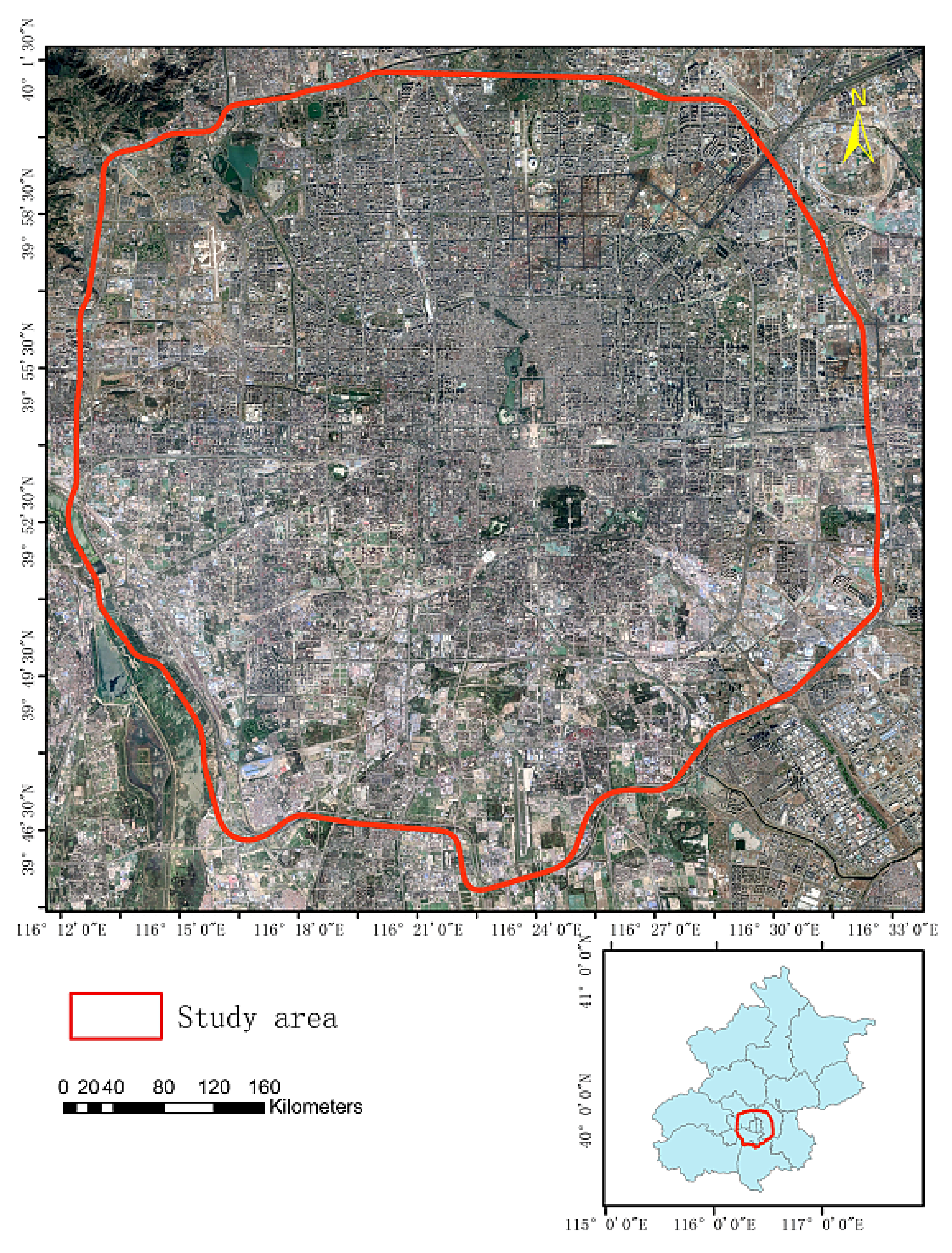
Beijing, the capital of China, has a large population and frequent population movement. Commuting trips have characteristics of strong temporal and spatial regularity and rigidity [44], which is the most important form of population activity in urban areas. According to the data provided by the Beijing Transport Institute, there are 23 million daily commuting trips on average, the average commuting distance is 12.4 km, and the average commuting time is 56 minutes. With the rapid progress of urbanization, Beijing has gradually formed an approximate radial and concentric spatial structure defined by ring roads [45]. There are 6 existing ring roads in Beijing, of which the Fifth Ring Road is a circular highway with a total length of 98.58 km. The area inside the Fifth Ring Road (Figure 1) is 667 square kilometers and includes Xicheng District, Dongcheng District, Chaoyang District, Haidian District, and Fengtai District, as well as most of Shijingshan District and the northern part of Daxing District. As Beijing’s core area, the area within the Fifth Ring Road has the highest population density and traffic flow [46]. According to the distribution of the permanent population in Beijing, jointly released in 2015 by the Beijing Municipal Bureau of Statistics and the Beijing Survey Team of the National Bureau of Statistics, the area within the Fifth Ring Road only accounts for 4.07% of the area of Beijing, while accounting for 49% of the permanent population in Beijing. Considering that the area encompassed by the Fifth Ring Road has a large population and regular population mobility, it is very suitable for the intraday variation mapping of population age structure. Therefore, we choose this area as the study area.
2.2. Data
2.2.1. Remotely Sensed Data
Four kinds of remotely sensed data were used in this article, which were used to generate covariates in the population dasymetric model of elderly individuals and children.
The Visible Infrared Imaging Radiometer Suite (VIIRS) (https://ncc.nesdis.noaa.gov/VIIRS/ accessed on 18 February 2021) onboard the Suomi National Polar-orbiting Partnership [47] spacecraft can produce a suite of average radiance composite images using nighttime light data from the VIIRS Day/Night Band (DNB) [48]. These data can identify weak light sources, which can be used to study the atmosphere, surface processes, and human activities. The VIIRS products have a spatial resolution of 740 m and are produced monthly and annually.
The land use and land cover data were obtained from the MODIS Land Cover Type Product (MCD12Q1) (https://lpdaac.usgs.gov/ accessed on 18 February 2021), which supplies global land cover maps at annual time steps and 500 m spatial resolution from 2001 to present. On the basis of the International Geosphere-Biosphere Program (IGBP) classification scheme, we divided the MCD12Q1 products into 17 land cover types. We selected categories related to population distribution and generated covariates used in the dasymetric model.
We collected digital elevation data from the Shuttle Radar Topography Mission (SRTM) (https://www2.jpl.nasa.gov/srtm/ accessed on 18 February 2021) to generate covariates related to topography. The resolution of the SRTM dataset is 1 arc-second (approximately 30 m). Most parts of the world have been covered by this dataset, ranging from 54° S to 60° N latitude, including Africa, Europe, North America, South America, Asia, and Australia. SRTM was used to generate topography-related variables, such as elevation and slope.
Sentinel-2 is a wide-swath, multispectral, and high-resolution Earth observation mission from the European Space Agency’s Copernicus Program. The mission supports a broad range of services and applications, such as agricultural monitoring, emergency management, land cover classification, and water quality [49]. The spatial resolution of each band of Sentinel-2 is shown in Table 1. Sentinel-2 was used to calculate some spectral indexes in this article.
2.2.2. Geospatial Data
Two types of geospatial data were used in this article, namely, OpenStreetMap (OSM) data and point of interest (POI) data.
OSM (https://www.openstreetmap.org/ accessed on 18 February 2021) is a collaborative project to create a free editable map of the world. As the most popular volunteer geographic information (VGI) project, OSM allows users to extract and upload data from handheld GPS devices, aerial photographs, other free content, or even local knowledge alone. This makes the OSM data crowdsourced and characterized by fast updates. OSM data also have the characteristics of high accuracy, and many studies have proven that the level of detail and coverage of their data is even better than some proprietary maps of certain countries or regions [50,51]. At the same time, since OSM has been proven to have a high positional accuracy in urban areas [52], it has been confirmed that it can be use in urban functional region (UFR) identification [53] and population mapping [27]. The OSM dataset was used in this article to identify the UFRs and to generate covariates for population dasymetric mapping.
The POI data were retrieved from NavInfo, the leading locational big data provider in China. POI data are a type of geospatial big data containing information such as names, coordinates, and categories. In recent years, many studies have demonstrated the usefulness of POI data in identifying UFRs [54,55,56,57,58,59] and population mapping [17,27,60]. In this article, POI data were also used in both UFR identification and population dasymetric mapping. A total of 230,329 records of POIs were obtained in the study area.
2.2.3. Demographic Data
The 2018 demographic data for Beijing were obtained from the China Statistical Yearbook published by the National Bureau of Statistics of China, which is the latest population data released thus far. The demographic data from 16 districts and counties of Beijing include the number of people in 3 age groups: 65 years old or older, 14 years old or younger, and 15 to 64 years old, which indicate the population at the end of the year. On the basis of these data, we calculated the proportion of elderly individuals and children and used this as the dependent variable in the permanent resident population dasymetric model.
2.2.4. Population Survey Sampling Data
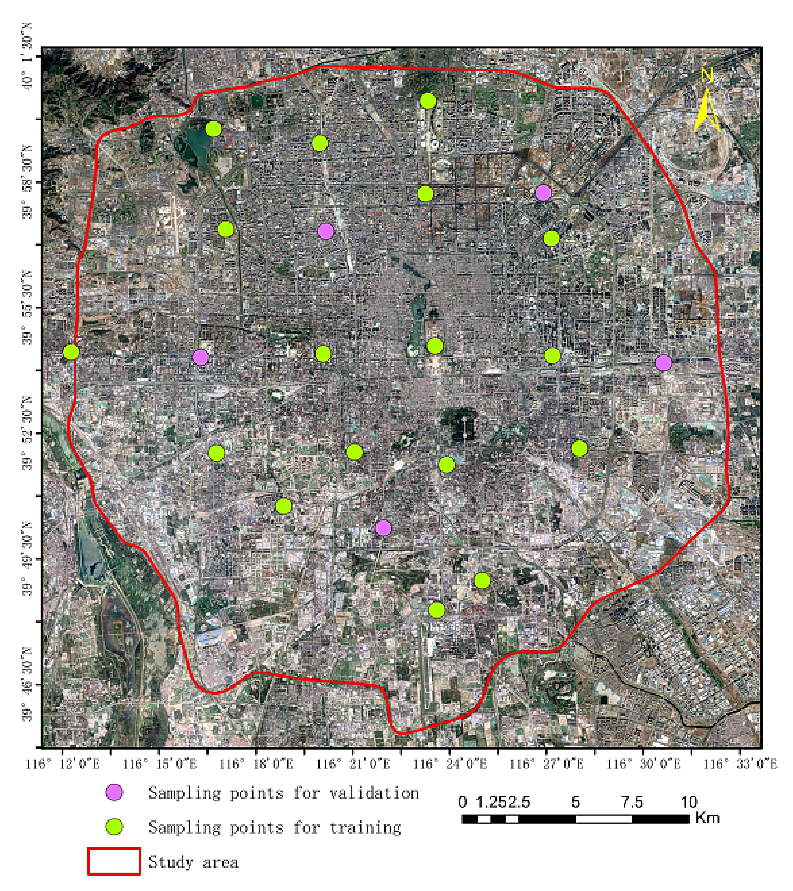
Population survey were organized on August 13 to 29, 2020. A total of 22 sampling points within the Beijing Fifth Ring Road (Figure 2) were deliberately selected evenly on the basis of the distribution of UFRs to ensure that each category of UFR could be sampled. The identification of UFRs is explained in detail below in Section 3.2.1. We conducted 6 population surveys in the morning, afternoon, and evening on weekdays and weekends at each sampling point. Two 5-minute demographic sampling videos were taken for each survey, with a 5-minute interval between the 2 videos. The video was shot with a GoPro Hero 7 Black action camera, which has HyperSmooth and Superview functions to shoot a smoother video with a wider field of view. We used these 2 functions to shoot videos with a resolution of 2.7 k, ensuring that we obtained population information as accurately as possible. From these videos, we were able to obtain data on the proportion of the population of different age groups at these sampling points. These data can represent the most accurate proportion of the population of each location in different time periods.
3. Methods
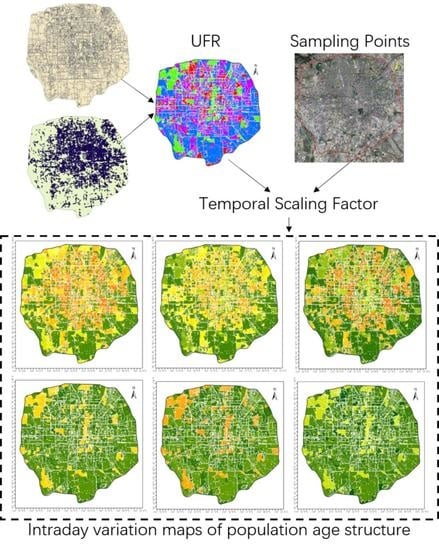
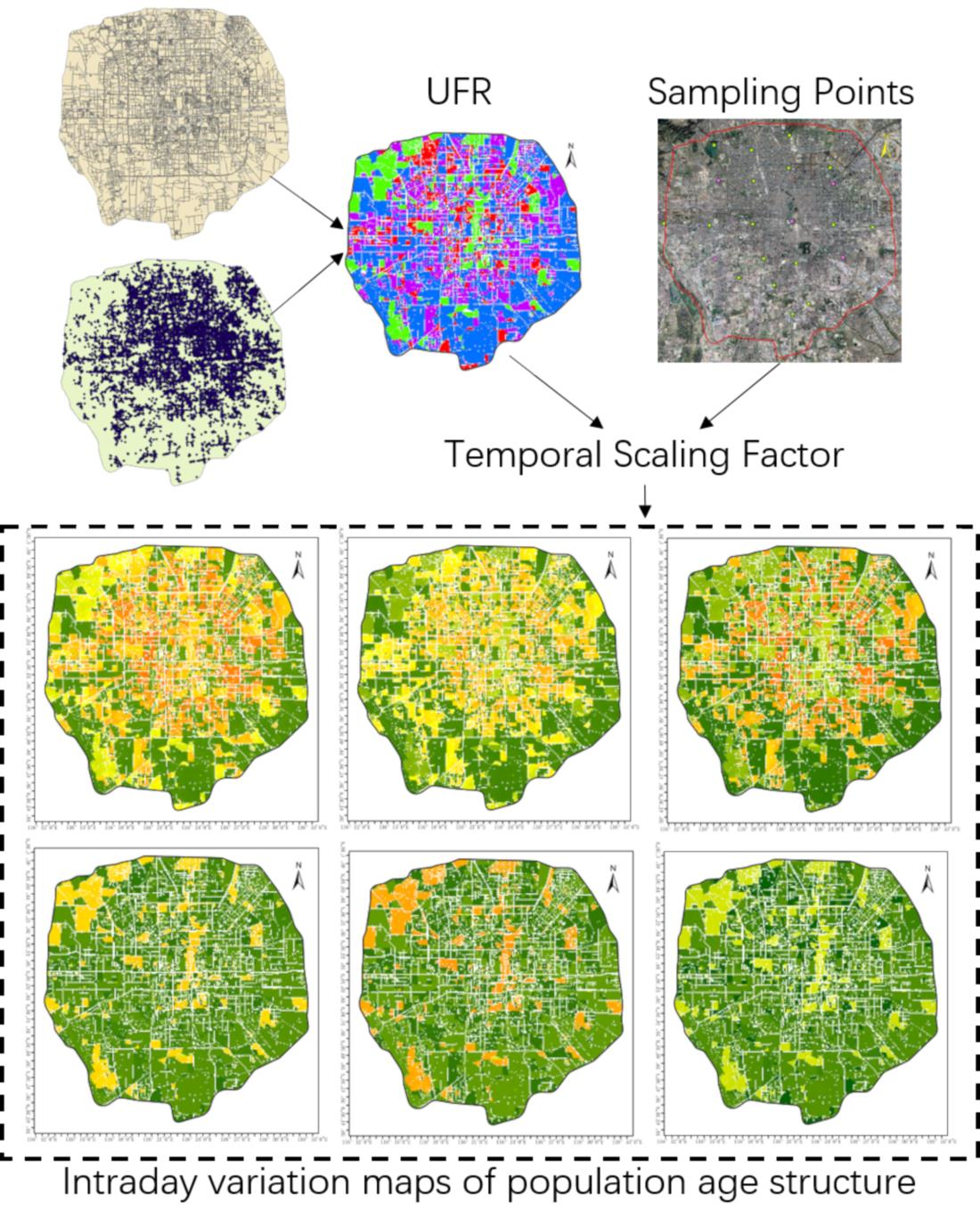
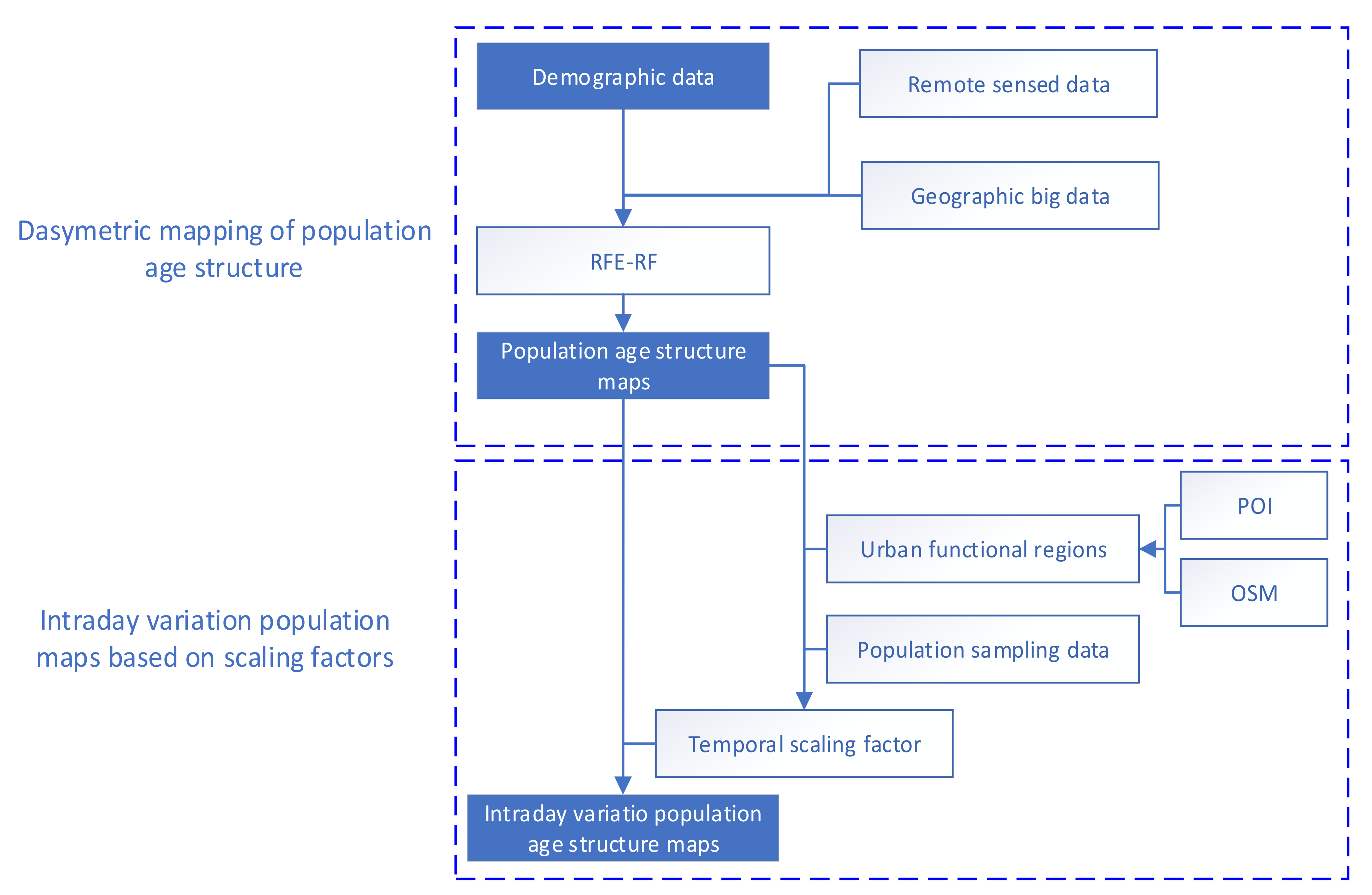
This section introduces the methods (Figure 3) used in this article. The purpose of this process was to generate intraday variation population maps of different age groups. According to common international practice, the population is usually divided into 3 groups according to age, namely, 0–14 years old for children, 15–64 years old for youth and adults, and 65 years and older for elderly individuals [61,62,63]. This article aimed to construct proportion maps and determine the mobility patterns of 2 age groups (children and elderly individuals). The overall process can be divided into 2 parts, namely, dasymetric mapping of the population age structure and intraday variation mapping of the population age structure, in order to realize the transformation of population data from demographic data to spatial data and from spatial data to spatiotemporal data. In the first part, the random forest-recursive feature elimination (RF-RFE) algorithm was used to select the optimal subset of covariates and perform dasymetric population mapping. In the second part, UFRs were identified using point of interest (POI) records and OpenStreetMap (OSM) data, and the temporal scaling factors were calculated by combining population sampling data. Temporal scaling factors were used to generate intraday variation maps of the elderly individuals and children.
3.1. Dasymetric Mapping of Population Age Structure
The accuracy of the dasymetric model depends on the covariates it used. Many factors, such as socioeconomic, physical (topographic, climatic, and environmental), and political factors [64,65], can affect (directly or indirectly) the distribution of the population [39]. Therefore, we calculated the covariates related to these factors. However, these factors need to be filtered in order to simplify the model and eliminate interference factors. Therefore, the dasymetric mapping of the population age structure consists of 2 parts: optimal subset selection of covariates and dasymetric modeling.
3.1.1. Covariates Calculation
During the past few decades, the rapid development of remotely sensed satellites and the popularization of smartphones has transformed the way we obtain ground information. The factors related to the population distribution introduced above can be obtained cheaply and effectively through remotely sensed data and geospatial big data. Remotely sensed data could be used to describe factors that include nighttime light data [66]; land use and land cover data [64]; topographic and landform data [67]; and remote sensing spectral indexes that evaluate vegetation, urbanization, and water bodies [33]. Geospatial data can reflect the topological relationship of spatial data. On the basis of these data, we calculated the following covariates related to population distribution.
Nighttime light data were found have strong population distribution associations in many studies [68,69]. Nighttime light data have been widely used in mapping the urbanization process [70,71] and mapping population age structure [39]. Thus, nighttime light data can be used as a basic covariate for estimating the distribution of the population age structure in urban areas. In this study, the VIIRS nighttime light composites for 2018 were obtained and preprocessed to filter out lights from fires, boats, the aurora, and other temporal lights.
Land cover information is usually selected to redistribute the aggregated census to improve the accuracy of gridded population data [64]. Land use and land cover data have a higher spatial resolution than census data, which can effectively improve the accuracy of population spatial modeling [72]. In particular, the built-up class has the closest relationship with the population distribution [27]. The urban and built-up land cover classes were extracted to generate the covariate of distance to built-up lands. We used the “Euclidean Distance” toll in ArcMap to generate raster data of the distance from the build-up area.
Topography is closely related to population distribution and even population change [73]. To analyze the relationship between topographical factors and the population’s age structure, we used STRM to generate two covariates, elevation and slope, in order to reflect the study area’s topographical factors. The “Slope” toll in ArcMap was used to generate raster data of the slope using STRM.
Remote sensing spectral indexes can effectively measure and monitor the ground features and have been proven to be related to population distribution [38,39]. Three indexes, the enhanced vegetation index (EVI), normalized difference built-up index (NDBI), and normalized water index (NDWI), were selected in this article. EVI, NDBI, and NDWI are 3 commonly used remote sensing indexes used to highlight vegetation, built-up areas, and water bodies. All 3 indexes were calculated from the Sentinel-2 MSI: Multispectral Instrument, Level-2A. We used the Google Earth Engine platform to calculate the average of these 3 indexes for the whole of 2018. The calculation formula for the three indexes are as follows:
The road network, river network, and water body data obtained from OSM were used in this article to identify UFRs and generate covariates in the population dasymetric model. Referring to the level information of road network data, we calculated 2 covariates, namely, road density and distance to road for each road category. At the same time, river network density and distance to the nearest water body were also used to analyze the impact of water bodies on population age structure distribution.
Dasymetric modeling by introducing POI data has been confirmed, reflecting the population distribution effectively [17,27,60]. In order to make full use of the relationship between POI records and population distribution, we also considered POI density and distance to POI for each category of POI in this study.
All the covariates introduced above were resampled to generate a 100 m resolution raster for dasymetric mapping, and these covariates are shown in Table 2.
3.1.2. Dasymetric Model Development
The dasymetric model has proven to be an effective method to generate gridded population maps. In this article, a new dasymetric model was established to generate fine-grained population maps of different age groups using the random forest (RF) model [74]. On the basis of the data presented above, we produced 50 covariates in this study. However, not all covariates can be used in dasymetric mapping. Therefore, to simplify the dasymetric model, remove the interference variables, and improve the model’s accuracy, we used the recursive feature elimination (RFE) [75] algorithm to select the optimal covariates subset used in the dasymetric model.
The RF model is a nonparametric model that has been widely used in classification or regression problems, and many scholars have used it for dasymetric mapping to reflect the natural distribution of human populations [25,76,77]. RF models grow a” forest” with numerous decision trees, and each tree is constructed using a random subset of the independent covariates and a random sample of the training dataset. The results were determined by all the trees in the “forest”. The process of randomly selecting data is called the bootstrap sampling technique. Data not selected in the bootstrap process are called out-of-bag (OOB) data, the OOB error estimation is an error estimation method that can replace that using the test set. The RF model has the advantage of having fewer adjustment parameters and can be applied to large datasets with high efficiency, which makes RF an ideal model for population dasymetric mapping.
RFE is a feature selection method that fits a model and removes the weakest features until the specified number of features is reached. It optimizes the model through multiple iterations, continuously removing features and rebuilding it on the remaining features. The importance of features is measured, and the less relevant features are removed at each iteration [78]. The RFE algorithm provides good performance with moderate computational efforts in finding the subset of features with the minimum possible generalization error [75,78].
In this study, the RF model used the population proportion of elderly individuals and children as the response variable and the mean value of each covariate selected by the RFE algorithm as the independent variables. The log-transformed process was used for each variable to generate a more regular and evenly distributed map [25]. Subset selection, model estimation, and prediction were performed using the free software environment R 3.6.1, which is used for statistical computing and graphics [79]. Two packages, randomForest [80] and caret [81], were used to generate the population dasymetric map.
The random forest algorithm has two parameters that need to be adjusted. After many experimental training repetitions, we finally decided that a 500-tree forest with 4 covariates for each tree could obtain a stable, minimized OOB error of prediction.
The RFE algorithm in the caret package was used in selecting the optimal subset of covariates. In this article, we produced a total of 50 covariates; hence, we screened out the best subsets containing 1-50 covariates and selected the optimal subsets from these subsets. Since this article used the random forest model for dasymetric modeling, we chose the rfFuncs for the rfeControl parameter in RFE algorithm.
The root mean square error (RMSE) was used to select the optimal subset, and the formula is as follows:
where represents the estimated value of county i; represents the true value obtained from demographic data; and N represents the number of counties here, which was 16.
The log-transformed variables were used in the population dasymetric model. To obtain the real population age structure maps, we back-transformed the result generated by the population dasymetric model to predict the population proportion for each pixel.
3.2. Temporal Scaling Based on UFR-Specific Mobility Pattern
3.2.1. Urban Functional Region Identification
The identification of UFRs consists of 2 steps, identify land-use parcels and determine the UFR category of each land-use parcel. Studies have shown that the segmentation of cities through multilevel road networks can obtain satisfactory results of regional boundaries [55,59,82,83]. POI data have also been proven to play an important role in land-use classification on the basis of human activities [54,56]. This paper proposes a UFRs identification method based on fine-scale parcel boundary data generated from OSM road network data and POI data.
A method proposed by Liu and Long [82] was adopted to identify land-use parcels. The OSM roads were first extended by 100 m to address the disconnection of the road network. The dangling roads and independent sections of the road network were then removed because they cannot be connected to nearby roads. Finally, the OSM roads were divided into 3 types according to the principal tags, and buffers of different distances were set for different types of roads. On the basis of the investigation of road width in the study area and the national standard in the Code for Design of Urban Road Traffic Facility issued by the Ministry of Housing and Urban-Rural Development of the People’s Republic of China, we generated buffers of 40, 20, and 10 m for Level 1 roads (highways and major roads), Level 2 roads (secondary roads), and Level 3 roads (third roads and fourth roads), respectively, in order to build an independent road space. The land-use parcels were built by removing the road space from the study area.
After the land-use parcels were identified, the POI data were used to determine each land-use parcel’s UFR category. There are 17 categories of POI data used in this article: carting, residential community, wholesale and retail, automobile sales and service, financial services, educational services, health and social security, sports and leisure, communal facilities, commercial facilities and services, resident services, corporation enterprises, transportation and storage, scientific research and technical services, agriculture, forestry, animal husbandry, and fisheries. It was necessary to reclassify the POI records since the POI data in this article will identify UFRs and these UFRs will serve population age structure mapping. All the POI records were merged into 4 categories: open space, industry and commerce, public service, and residential. These 4 reclassified categories can clearly reflect the population mobility pattern and can serve for spatiotemporal population age structure mapping [42]. The kernel density of these 4 categories of POIs was calculated to determine the land-use parcels’ UFR category. The kernel density is estimated on the basis of the first law of geography, that is, the closer the location is to the core element, the greater the density expansion value it obtains, which reflects the characteristics of spatial heterogeneity and the attenuation of center strength with distance [84]. This makes full use of the original data information, and the result is less affected by subjective factors and has the advantages of gradual change and revealing detailed characteristics, which makes it possible to reveal the details of things and realize the spread of radiation effects on neighboring locations.
Therefore, each land-use parcel’s category was judged by the kernel density of POIs. This process of determining the category of land-use parcels consists of 2 steps. First, calculating the kernel density of the 4 POI categories and all POIs in each land-use parcel, if the density of a certain POI category exceeded 50% of the density of all POIs, we regarded the category of this POI as the category of this parcel. Second, for mixed parcels that did not have an absolute advantage POI category, further operations were needed to determine the category of these parcels. Near-convex-hull analysis (NCHA) was used to reclassify POI in land-use parcels [46]. For example, industrial and commercial POI records such as stores will be located in parks, which interferes with the identification of open space UFR identification. In order to eliminate similar interference, these industrial and commercial POIs should be reclassified as open space POI through NCHA. The specific operation is as follows. The convex hull (the minimum polygon boundary) of the most numerous POI category in each parcel was calculated. Then, the other POIs in this convex hull were reclassified into this category, and the first step was repeated to identify the category of these parcels. Finally, null values were assigned to parcels that were still unidentifiable.
3.2.2. Temporal Scaling Factor Calculation
The population age structure map can be generated on the basis of the urban functional map, the population dasymetric maps of different age groups, and the population survey sampling data. This process consists of two steps. The first step is to calculate the temporal scaling factors (TSFs) of different age groups in different UFRs at different time periods. The second step is to calculate the intraday variation population age structure map on the basis of the temporal scaling factors.
It has been proven that human mobility pattern has strong spatiotemporal regularity, and these regularities can be used to reveal the relationship between different UFRs of the city [85,86]. Therefore, the population mobility patterns are consistent for the same category of UFRs, and the TSFs of the same UFR should also be the same. To calculate these TSFs, we divided the 22 sampling points introduced above into training data (17) and validation data (5). We calculated the TSFs for different people in different time periods in each category of UFR according to the population dasymetric map and the training data. The calculation formula for the TSFs of the elderly and children in different time periods and different categories of UFRs is as follows:
Among them, represents a certain type of people in a certain category of UFR at a certain time period, represents the measured proportion of the j-th sampling point in this kind of UFR, and represents the value of the same point in maps generated by dasymetric mapping. The variable represents the statistical population value of the j-th sampling point in this kind of UFR, and represents the total number of populations in the same kind of UFR in the same time period.
4. Results
4.1. Dasymetric Maps of Population Age Structure
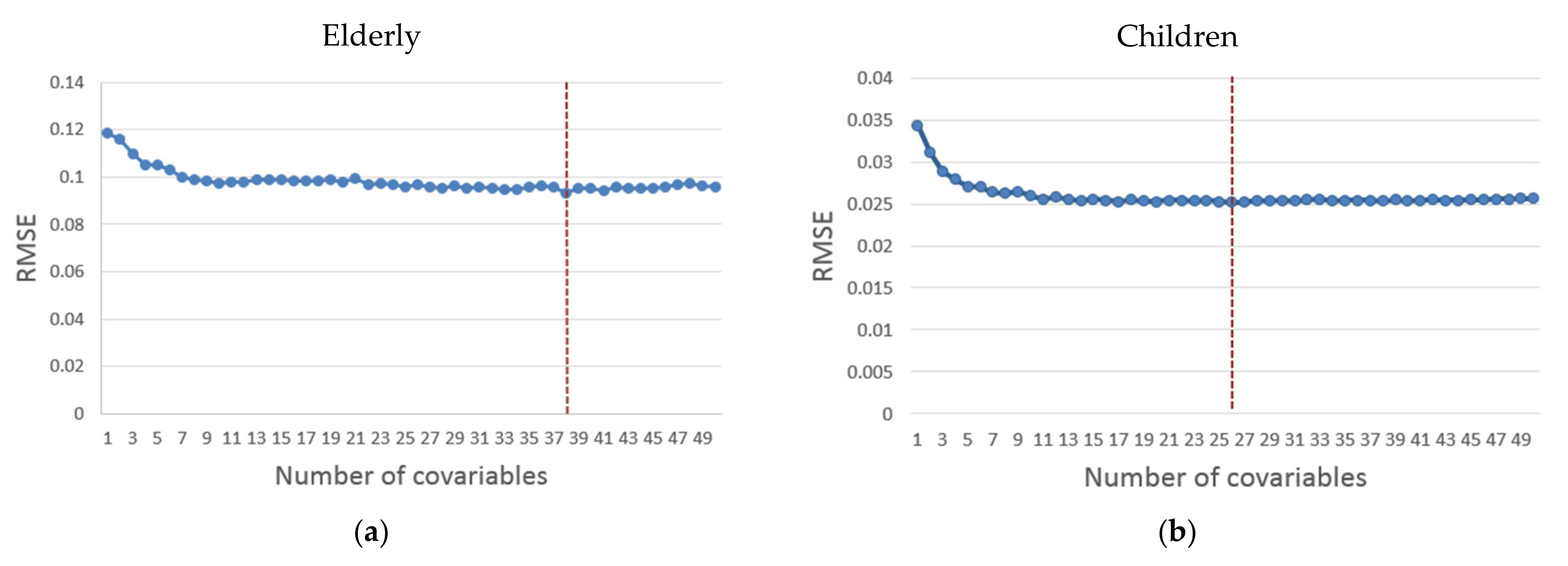
Optimal subset covariate selection was driven by the RFE algorithm using county-level demographic data and the average value of 50 covariates in each county. We screened out the optimal subset containing 1 to 50 covariates for dasymetric models for the elderly individuals and child populations proportionally.
The indicator of each optimal subset is shown in Figure 4. RMSE was used as the indicator to select the optimal subset of the population dasymetric model. The subset with the smallest value is the optimal subset. Finally, the optimal subset containing 38 covariates and 26 covariates was selected for population dasymetric model of elderly individuals and children, respectively.
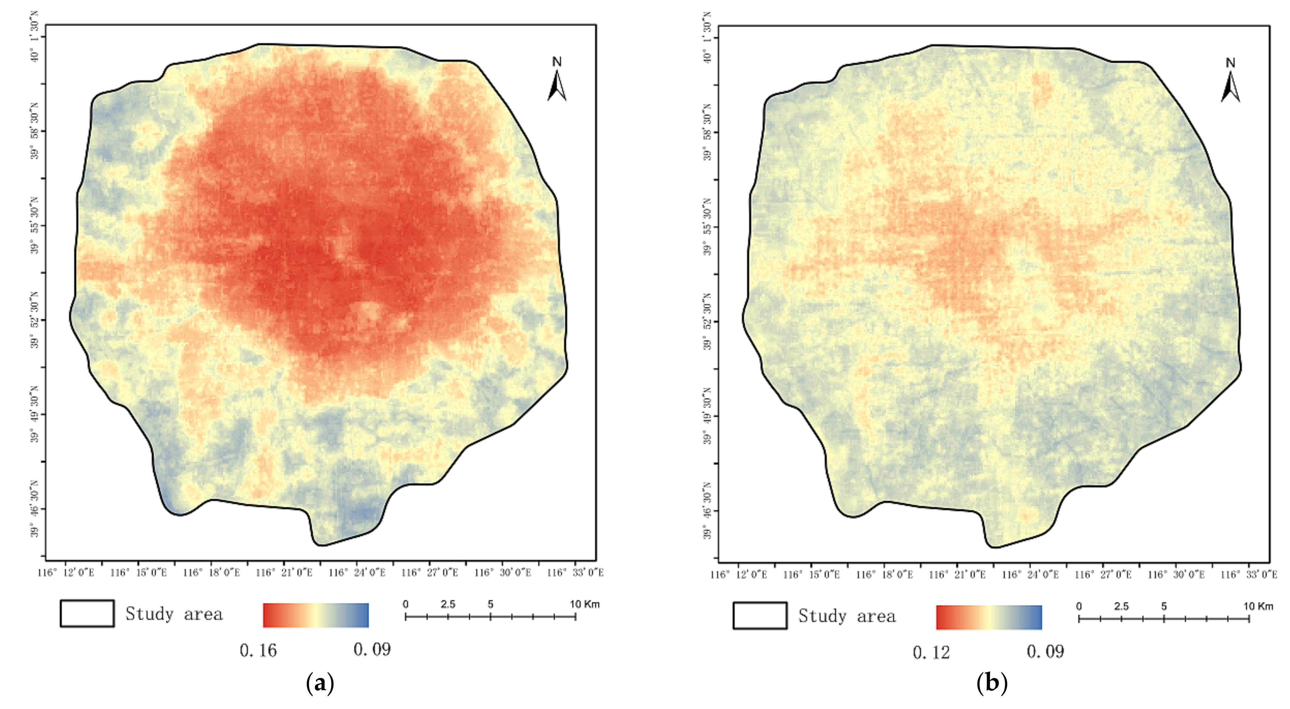
An RF-based dasymetric model was constructed with the above covariates described in Section 3.2.2, which was used to downscale the proportion of different age groups of people in each county. The fine-gridded population dasymetric map at a 100 m spatial scale in the experiment showed visually satisfactory results (Figure 5). Figure 5a shows the dasymetric map of the elderly individuals’ proportion, while Figure 5b shows the dasymetric map of the children proportion. The accuracy of the RF-based dasymetric model was evaluated using . The results show that the values of the population maps of elderly individuals and children were 98.14% and 91.54%, respectively. This proves that the dasymetric model using the optimal subset covariates selected by RFE can well represent the population distribution.
4.2. Urban Functional Region
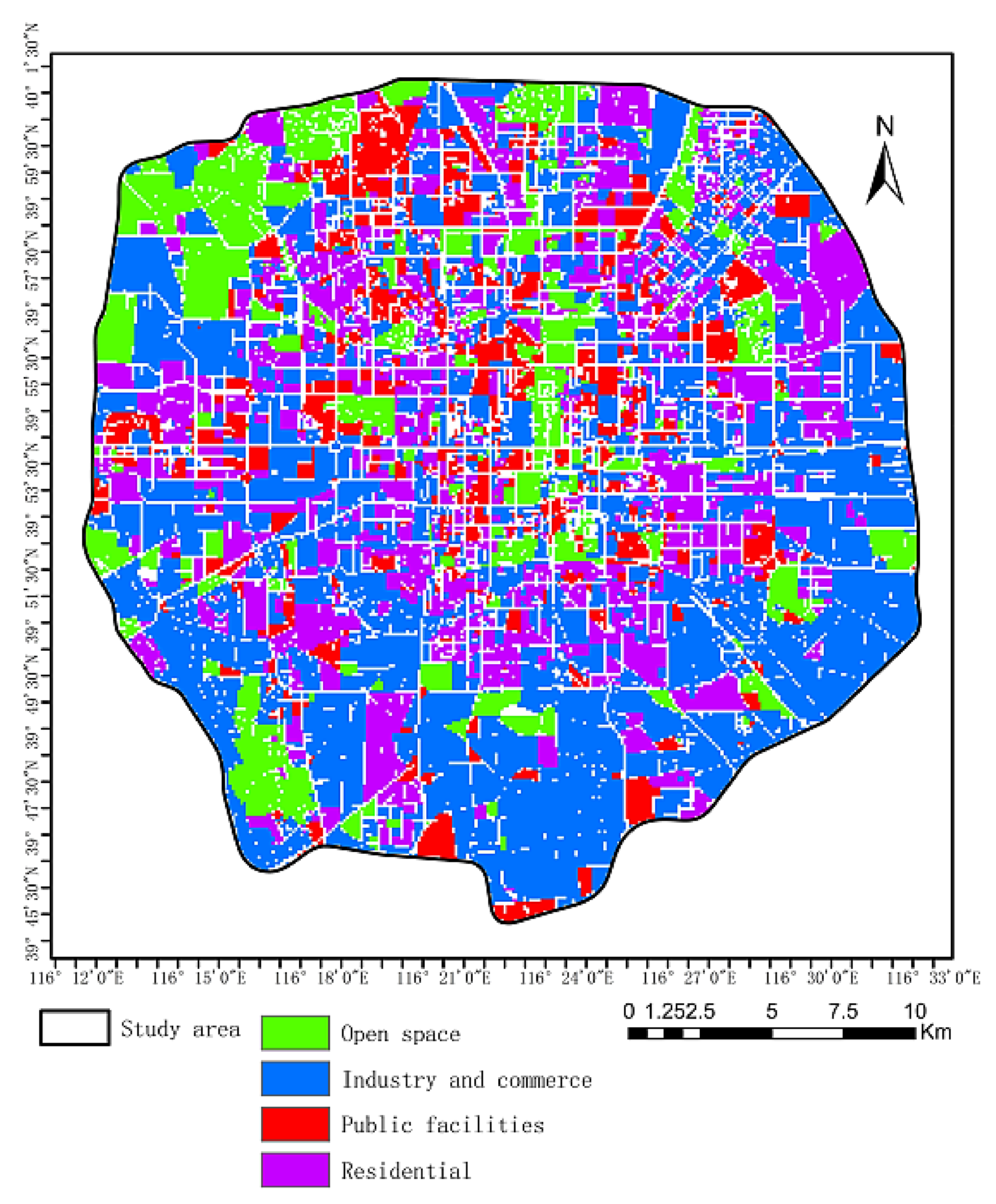
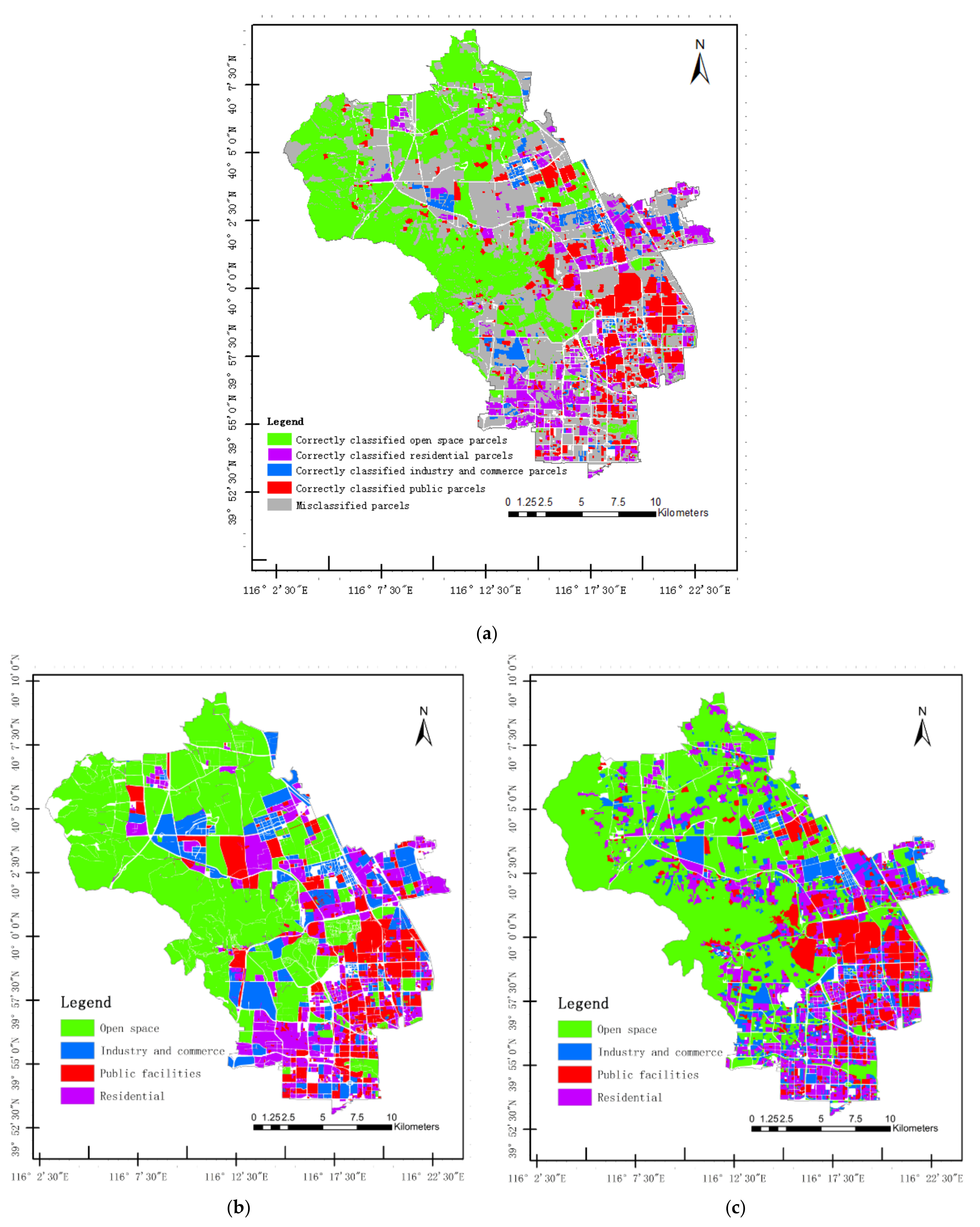
The UFRs within the Fifth Ring Road identified as described in Section 3.2.1 are shown in Figure 6. The actual boundary and category of UFRs was manually interpreted within a selected validation area of the study area (Haidian District within the Fifth Ring Road), with the assistance of a field survey, high-resolution remote sensing images, digital maps, and POI data. The actual UFRs were compared with the classification result for accuracy evaluation.
The confusion matrix for the UFR identification result is shown in Table 3. The identification result achieved an overall accuracy of 70.97%. Of all the four UFR categories, open space and public categories had the highest identification accuracy, with both the user’s and producer’s accuracies above 72%. However, the identification accuracies of industry and commerce facilities, and residential categories were relatively low, especially for industry and commerce facilities, where the user’s and producer’s accuracies were only over 50%. This was mainly due to the relatively wide distribution of POIs in the industry and commerce facilities category, which is easy to mix with other POI categories and leads to confusion. For example, in open space UFRs where there are tourist attractions, there will also be restaurants, hotels, and other commercial facilities nearby. This has a great impact on its identification accuracy.
Figure 7a displays the correctly identified result of UFRs, while Figure 7b,c displays the UFRs identification result in this article and the visual interpretation result of UFRs, respectively. As shown in Figure 7, the distribution of open space category distributions, residential category, and public facilities category are relatively concentrated. They are distributed in the northwest, south, and east of the validation area. However, the industry and commercial facilities categories are relatively dispersed and distributed in the whole region, interweaving with the other three UFR categories, which further confirms the above analysis of the reasons for the poor accuracy of the identification results of industry and commercial facilities. This indicates that it is difficult to use only POI records when recognizing the industry and commercial facilities UFRs. They are easier to mix with other UFR categories and interfere with the accuracy of the overall UFRs identification result. Therefore, it is necessary to introduce other information, such as spectral and texture features and landscape metrics, in order to improve these mixed regions’ identification accuracy. The specific process will be discussed in detail in the conclusions and discussion.
There is an inherent limitation in land-use parcels generating using road network data. The land-use parcels’ boundary derived from the OSM road data was different from that of manual interpretation, and many small parcels were not recognized. This is usually associated with the under-segmentation phenomenon. In reality, land-use parcels are not only segmented by road networks, but rather walls, fences, trees, or even nothing [59]. Segmentation using only road network data will merge some small parcels into larger parcels, forming mixed UFRs and even misidentified the category of UFRs.
4.3. Temporal Scaling Factors of Different UFRs
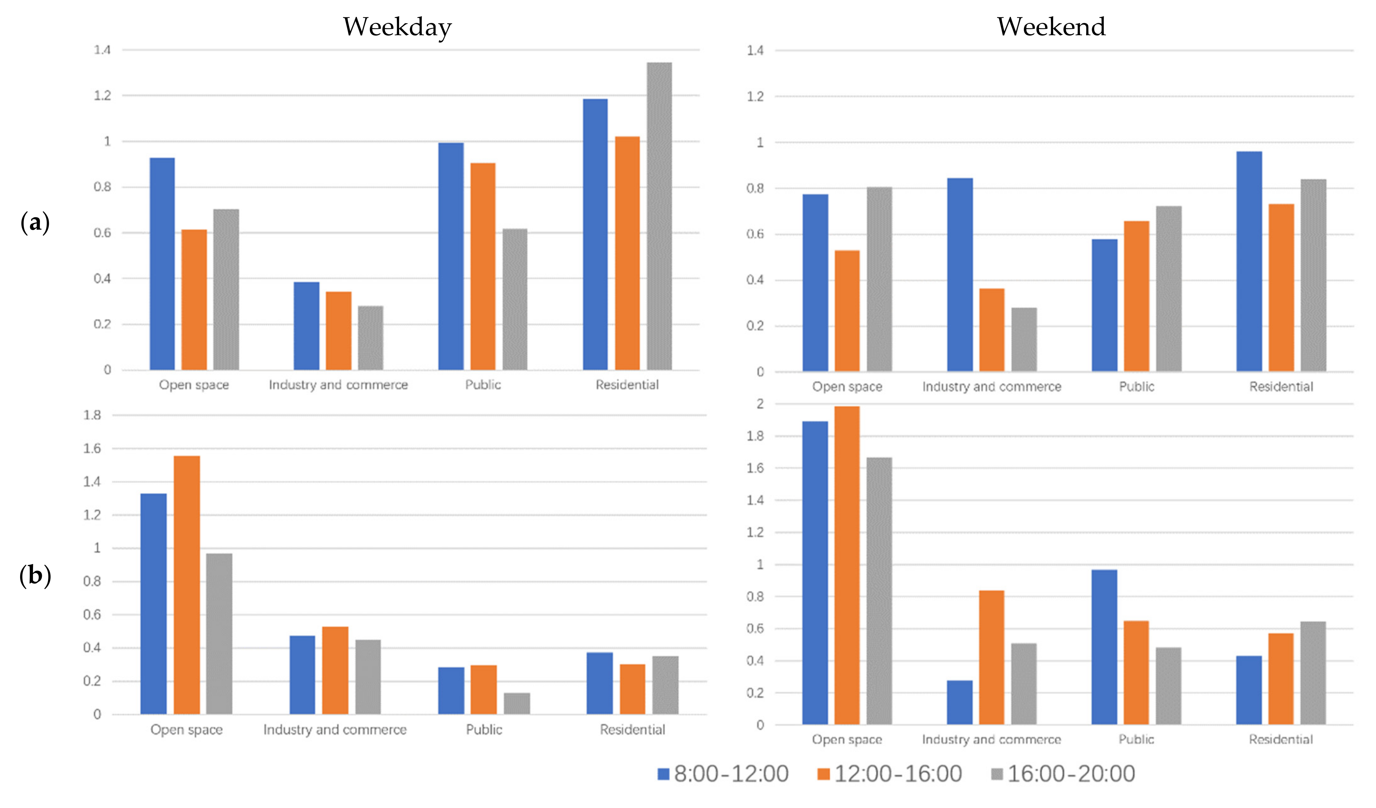
The temporal scaling factors of each category of UFR on weekdays and weekends was calculated. The result of these scaling factors is shown in Figure 8. In addition to being used in intraday various mapping of elderly individuals and children, these factors can also be used in analyze the mobility patterns and distribution preferences. On the basis of these temporal scaling factors, we can obtain the following three conclusions.
First, elderly individuals and children had different activity preferences and distribution characteristics. The proportion of elderly individuals in residential UFRs was usually higher, while the proportion of children in open space UFRs was higher. This was mainly due to the attributes of the elderly and children. Elderly individuals usually need a small amount of activity; hence, they are usually distributed near their homes. In contrast, children usually need a larger amount of activity, and thus they often go to parks, playgrounds, and other open-space UFRs.
Second, the distribution of different age groups in different time periods of the day had certain patterns. Except for residential UFRs on weekdays and public facilities UFRs on weekends, the time period with the highest proportion of elderly individuals was between 8:00 and 12:00. However, for children, apart from residential UFRs on weekdays and public facilities and residential UFRs on weekends, the time period with the highest distribution ratio was usually between 12:00 to 16:00. This shows that elderly individuals were more willing to perform activities in the morning, while children were more willing to perform activities in the afternoon.
Third, the distribution of different groups of people on weekdays and weekends had a certain pattern. Compared with weekdays, the proportion of elderly individuals in residential UFRs on weekends was significantly reduced, and the temporal scaling factors dropped by 0.23, 0.29, and 0.51 in the morning (8:00–12:00), afternoon (12:00–16:00), and evening (16:00–20:00), respectively. For children, the temporal scaling factor in both open space and public facilities UFRs was increased. The temporal scaling factor of open space UFRs increased by 0.56, 0.43, and 0.7 in the morning, afternoon, and evening, respectively. On the other hand, the temporal scaling factor of the public facilities UFRs increased by 0.69, 0.35, and 0.35 in the morning, afternoon, and evening, respectively.
4.4. Intraday Variation Maps of Population Age Structure
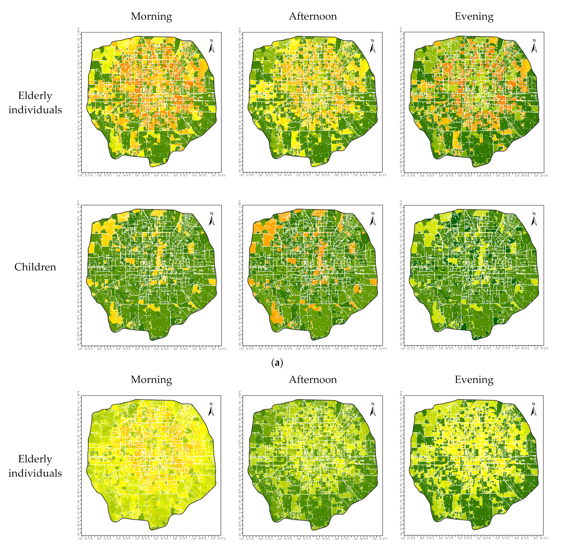
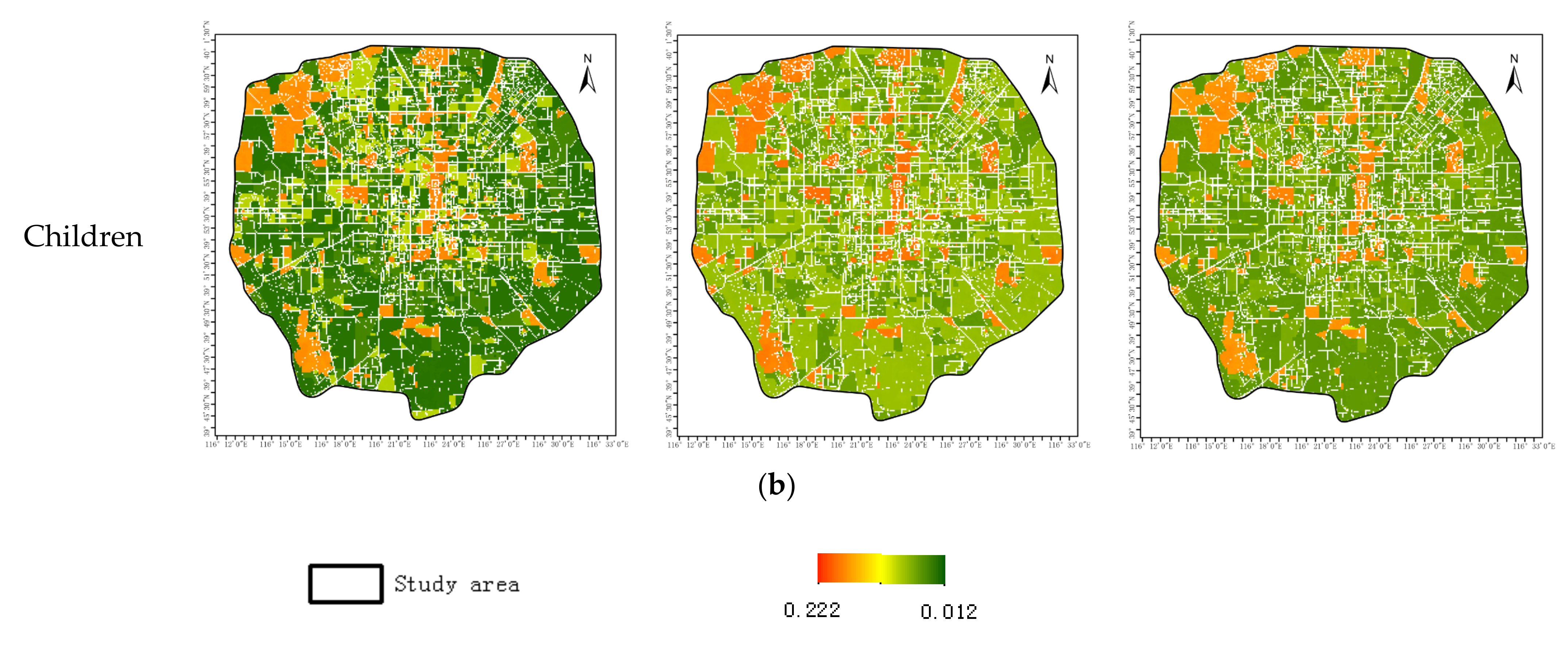
According to the population proportion maps of elderly individuals and children calculated in Section 4.1 and the temporal scaling factors calculated in Section 4.3, we were able to obtain the following fine-resolution intraday variation population maps of elderly individuals and children of weekdays (Figure 9a) and weekends (Figure 9b). As shown in these maps, the proportion of the elderly population was higher than that of children in all time periods in residential and public facilities UFRs. In comparison, the proportion of children was higher than that of elderly individuals in almost all open space UFRs at all times. In industry and commerce facilities UFRs, except for weekday and weekend mornings, the proportion of children was higher than that of the elderly. This also confirms, to a certain extent, the regularity of activities of the elderly and children. Children prefer outdoor sports and entertainment, and they will gather more in open space and industry and commerce facilities UFRs. On the other hand, the elderly individuals are more willing to participate in public activities, and they will gather more in residential and public facilities UFRs.
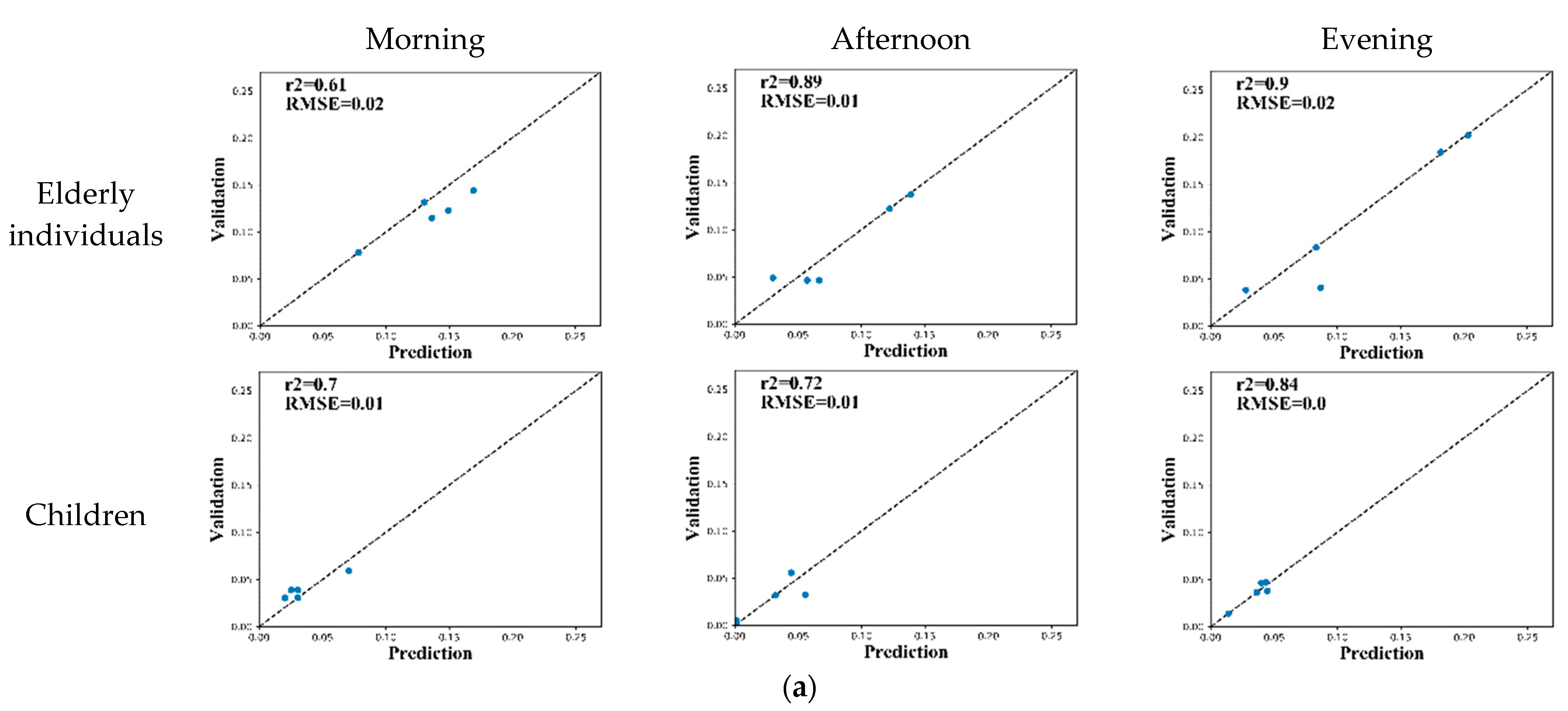
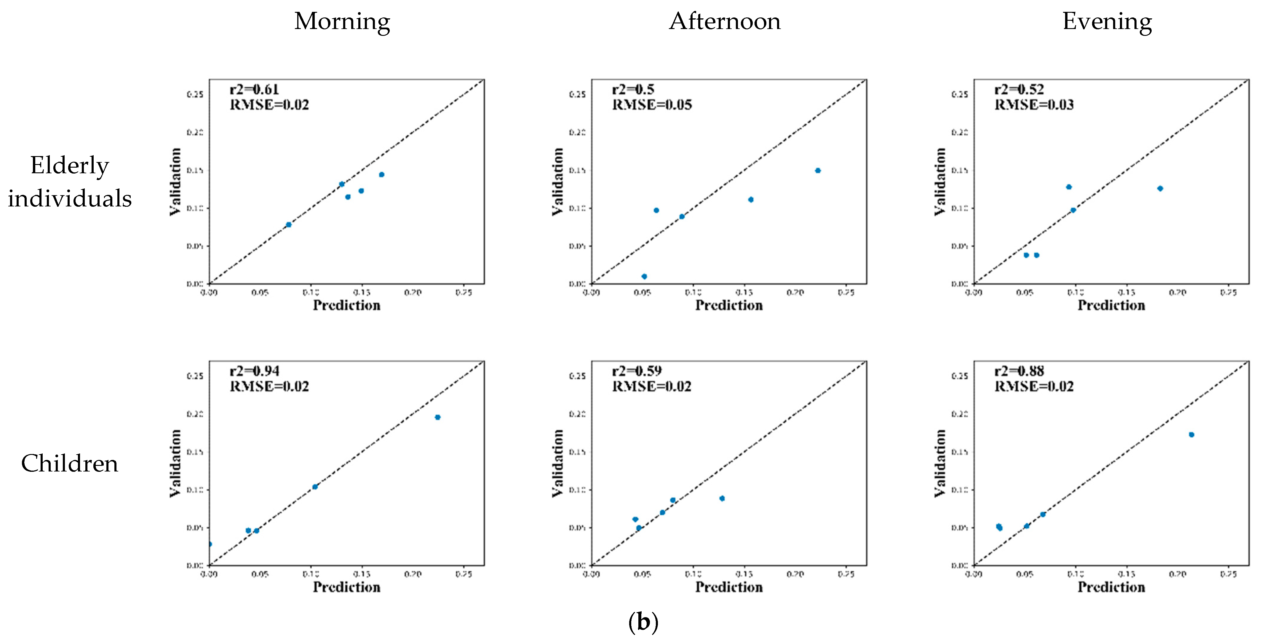
The accuracy of these intraday variation maps of population age structure was evaluated on the basis of the five sampling points for validation introduced in Section 2.2.4. We used the and RMSE indicators to evaluate the accuracy of the result (Figure 10). The result showed that the accuracy of the intraday variation maps on weekdays was higher, with the of elderly individuals and children in different time periods all above 0.6 and the value of the RMSE less than 0.02. However, the accuracy of the intraday variation maps on weekends was relatively low, with only higher than 0.5 and RMSE less than 0.05. The reason for this phenomenon may be that middle-aged people are more active on weekends, and they account for a relatively high proportion of the population, which interferes with the accuracy of intraday variation mapping of the elderly and children. At the same time, after comparing the prediction accuracy of different periods of the day, we found that the prediction accuracy in the evening was the highest. This may have been because people’s mobility in the evening will be lower than that during the day [27,87], and low population mobility makes the population distribution relatively fixed, which is conducive to improve the accuracy of population distribution estimation.
5. Discussion
The first advantage of this article is that we innovatively used UFR data and introduced the temporal scaling factor’s concept to produce fine resolution intraday variation maps of population age structure to overcome MAUP in population maps. We first achieved high accuracy UFR identification using road network data and POI data. Then, we innovatively proposed a dasymetric model based on the RF-RFE algorithm for the elderly and children. Finally, we calculated the temporal scaling factor using the population survey data and generated the intraday variation maps of population age structure. The second advantage of this article is our ability to analyze the activity patterns of population using these maps.
However, our study still had limitations and uncertainties, such as the intraday variation population maps’ low accuracy for weekend mornings and afternoons. To overcome these limitations and uncertainties, future research can consider the following aspects in order to improve population proportion maps’ mapping accuracy.
The first aspect is to further improve the identification accuracy of UFRs. Since the temporal scaling factor was calculated on the basis of the UFRs’ category, a higher UFRs’ identification accuracy may improve spatiotemporal population maps’ final accuracy. This article only used OSM road network and POI data to identify UFRs. Although the UFR identification results were reasonably good, with the overall accuracy reaching 70.97% (Table 3), there were still some shortcomings. For example, the identification accuracy of industry and commercial facility UFRs was low and needs to be further improved. The most direct way to improve the identification accuracy of UFRs is to introduce other data related to the division of UFRs, such as high-resolution remote sensing images and landscape metrics. High-resolution remote sensing images can provide many spectral and texture attributes that have already been used in UFR identification [88,89]. Landscape metrics have also been found to be a very important indicator in differentiating urban land uses [59,90,91]. Therefore, in the next step, we further introduce these data to improve UFR identification accuracy.
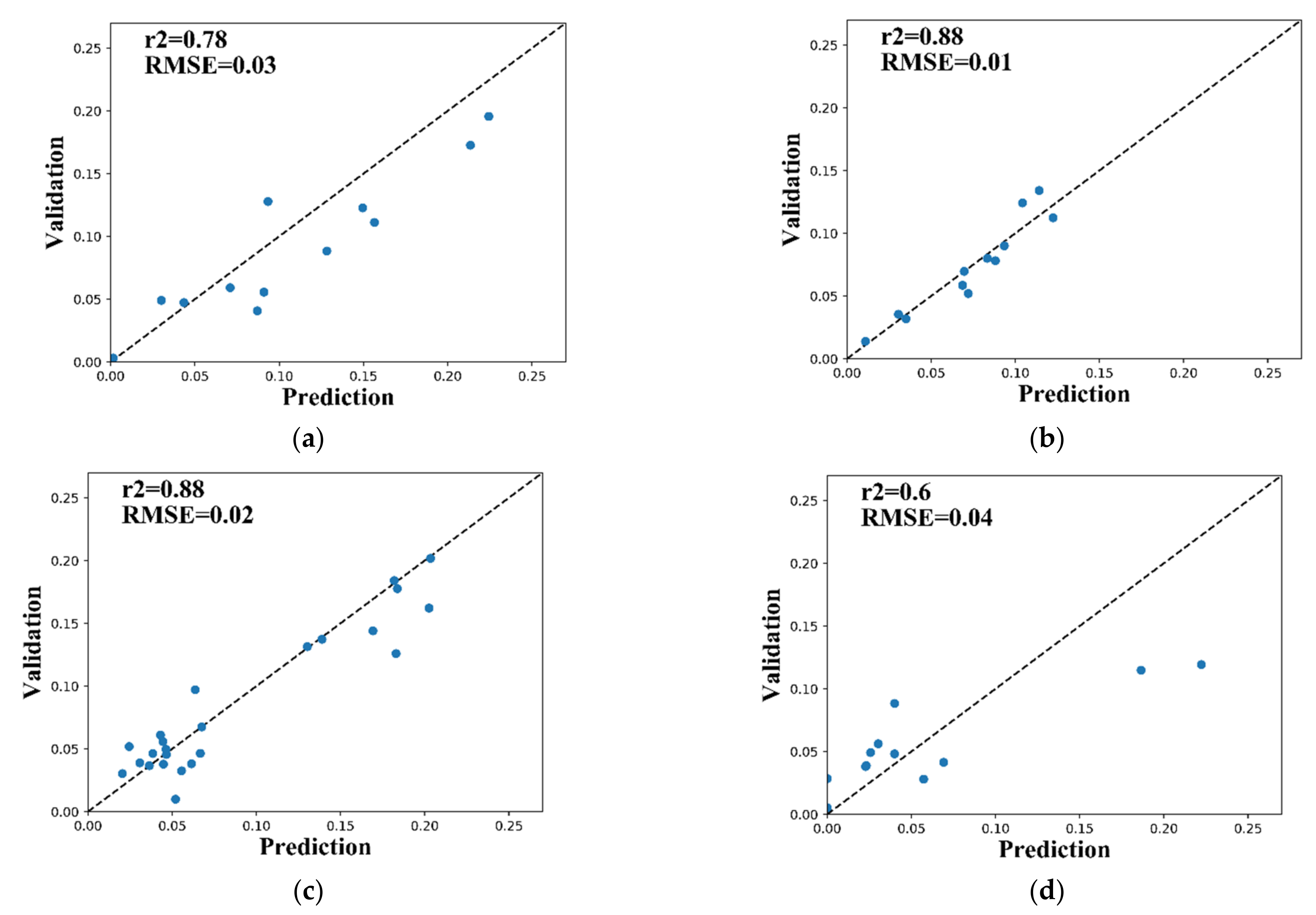
The second aspect is the city’s complexity; this article’s temporal scaling factor did not fully reflect the real situation. We divided the records from sampling points for validation into four categories according to the UFR categories and found that the accuracy of the records was less accurate in the industrial and commercial facility regions (Figure 11). This may have been due to the complexity of the industry and commercial facility regions themselves. It is necessary to further divide the industrial and commercial regions, such as the separation of industrial regions and commerce regions, in order to obtain more UFR categories so that this article’s research results are more realistic. In the future, more categories of UFRs will be identified to improve the accuracy of intraday variation population age structure mapping.
The third aspect is sampling error. Since the population is flowing and uneven, there may be abnormal values in the process of population sampling, such as the elderly tour group when sampling in tourist attractions, which will interfere with the population sampling results. In order to solve this problem, the number of sampling points and the sampling times of each sampling point can be increased to eliminate the sampling error as much as possible.
The last aspect is the inherent drawbacks with parcels generated using the road network data. In this article, we assumed that all the parcels were separated by roads. In reality, parcels in real life can be divided by walls, vegetations, river, or even nothing. Therefore, in future research, it is necessary to comprehensively consider these elements and establish a multi-element land-use parcels identification method to improve the identification accuracy of land-use parcels.
6. Conclusions
The objectives introduced in the introduction were achieved in this study. We realized the intraday variation mapping of population age structure, and also proved that the mobility of the urban population has certain patterns. People of different age groups will prefer to gather in a different category of UFRs at different periods.
This article made the first attempt to apply UFR data to analyze the spatial and temporal distribution of elderly individuals and children. The results of this article can accurately display information on the distribution and activity patterns of population of different age groups, which can be directly applied to assess the aging of the population in different regions and urban management. The research method in this article also provides ideas for calculating the proportion of other populations with different attributes (e.g., gender or income levels) in the future. The fine resolution intraday variation maps of population age structures in this article can be further used in many other studies. By combining the results of this article and population maps such as Worldpop and LandScan, we were able to obtain the distribution data of elderly individuals and children in different time periods. These data will play a vital role in the risk assessment of disasters, public health management, and many other aspects.
Author Contributions
Author Contributions: Conceptualization, Y.Z. (Yuncong Zhao), Q.L., and Y.Z. (Yuan Zhang); methodology, Y.Z. (Yuncong Zhao); software, Y.Z. (Yuncong Zhao); data acquisition and production Y.Z. (Yuncong Zhao) and J.Z.; writing—original draft preparation, Y.Z. (Yuncong Zhao); writing—review and editing, Y.Z. (Yuncong Zhao), Q.L., Y.Z. (Yuan Zhang), X.D., and H.W.; supervision, Q.L. All authors have read and agreed to the published version of the manuscript.
Funding
This research was funded by the Strategic Priority Research Program of the Chinese Academy of Sciences, grant number XDA 20030302.
Data Availability Statement
Public available datasets were analyzed in this study. These data can be found here: https://ncc.nesdis.noaa.gov/VIIRS/, https://lpdaac.usgs.gov/, https://www2.jpl.nasa.gov/srtm/, https://scihub.copernicus.eu, https://www.openstreetmap.org/, http://nj.tjj.beijing.gov.cn (accessed on 18 February 2021).
Acknowledgments
We thank the anonymous reviewers whose comments and suggestions significantly improved the manuscript.
Conflicts of Interest
The authors declare no conflicts of interest.
References
- Linard, C.; Tatem, A.J. Large-scale spatial population databases in infectious disease research. Int. J. Health Geogr. 2012, 11, 7. [Google Scholar] [CrossRef] [Green Version]
- Pindolia, D.K.; Garcia, A.J.; Huang, Z.; Smith, D.L.; Alegana, V.A.; Noor, A.M.; Snow, R.W.; Tatem, A.J. The demographics of human and malaria movement and migration patterns in East Africa. Malar. J. 2013, 12, 397. [Google Scholar] [CrossRef] [Green Version]
- Tatem, A.J.; Campiz, N.; Gething, P.W.; Snow, R.W.; Linard, C. The effects of spatial population dataset choice on estimates of population at risk of disease. Popul. Health Metr. 2011, 9, 4. [Google Scholar] [CrossRef] [PubMed] [Green Version]
- Tatem, A.J.; Garcia, A.J.; Snow, R.W.; Noor, A.M.; Gaughan, A.E.; Gilbert, M.; Linard, C. Millennium development health metrics: Where do Africa’s children and women of childbearing age live? Popul. Health Metr. 2013, 11, 11. [Google Scholar] [CrossRef] [Green Version]
- Forbes, V.E.; Calow, P.; Grimm, V.; Hayashi, T.I.; Jager, T.; Katholm, A.; Palmqvist, A.; Pastorok, R.; Salvito, D.; Sibly, R.; et al. Adding Value to Ecological Risk Assessment with Population Modeling. Hum. Ecol. Risk Assess. 2011, 17, 287–299. [Google Scholar] [CrossRef]
- Tang, X.; Li, Q.; Wu, M.; Tang, W.; Jin, F.; Haynes, J.; Scholz, M. Ecological Environment Protection in Chinese Rural Hydropower Development Practices: A Review. Water Air Soil Pollut. 2012, 223, 3033–3048. [Google Scholar] [CrossRef]
- Butler, D. Reactors, residents and risk. Nat. Cell Biol. 2011, 472, 400–401. [Google Scholar] [CrossRef] [PubMed]
- Mondal, P.; Tatem, A.J. Uncertainties in Measuring Populations Potentially Impacted by Sea Level Rise and Coastal Flooding. PLoS ONE 2012, 7, e48191. [Google Scholar] [CrossRef] [PubMed]
- Wegscheider, S.; Post, J.; Zosseder, K.; Muck, M.; Strunz, G.; Riedlinger, T.; Muhari, A.; Anwar, H.Z. Generating tsunami risk knowledge at community level as a base for planning and implementation of risk reduction strategies. Nat. Hazards Earth Syst. Sci. 2011, 11, 249–258. [Google Scholar] [CrossRef]
- Flowerdew, R. How serious is the Modifiable Areal Unit Problem for analysis of English census data? Popul. Trends 2011, 145, 106–118. [Google Scholar] [CrossRef]
- Dark, S.J.; Bram, D. The modifiable areal unit problem (MAUP) in physical geography. Prog. Phys. Geogr. Earth Environ. 2007, 31, 471–479. [Google Scholar] [CrossRef] [Green Version]
- Jelinski, D.E.; Wu, J. The modifiable areal unit problem and implications for landscape ecology. Landsc. Ecol. 1996, 11, 129–140. [Google Scholar] [CrossRef]
- Fotheringham, A.S.; Wong, D.W.S. The Modifiable Areal Unit Problem in Multivariate Statistical Analysis. Environ. Plan. A 1991, 23, 1025–1044. [Google Scholar] [CrossRef]
- Botta, F.; Moat, H.S.; Preis, T. Quantifying crowd size with mobile phone and Twitter data. R. Soc. Open Sci. 2015, 2, 150162. [Google Scholar] [CrossRef] [PubMed] [Green Version]
- Kovalcsik, T.; Szabó, B.; Vida, G.; Boros, L. Area-Based and Dasymetric Point Allocation Interpolation Method for Spatial Modelling Micro–Scale Voter Turnout in Budapest. Geogr. Technol. 2021, 16, 67–77. [Google Scholar] [CrossRef]
- Buzzelli, M. Modifiable Areal Unit Problem. Int. Encycl. Hum. Geogr. 2020, 169–173. [Google Scholar]
- Bakillah, M.; Liang, S.; Mobasheri, A.; Arsanjani, J.J.; Zipf, A. Fine-resolution population mapping using OpenStreetMap points-of-interest. Int. J. Geogr. Inf. Sci. 2014, 28, 1940–1963. [Google Scholar] [CrossRef]
- Holt, J.B.; Lo, C.; Hodler, T.W. Dasymetric Estimation of Population Density and Areal Interpolation of Census Data. Cartogr. Geogr. Inf. Sci. 2004, 31, 103–121. [Google Scholar] [CrossRef]
- Langford, M. Rapid facilitation of dasymetric-based population interpolation by means of raster pixel maps. Comput. Environ. Urban Syst. 2007, 31, 19–32. [Google Scholar] [CrossRef]
- Reibel, M.; Agrawal, A. Areal Interpolation of Population Counts Using Pre-classified Land Cover Data. Popul. Res. Policy Rev. 2007, 26, 619–633. [Google Scholar] [CrossRef]
- Lo, C.P. Population Estimation Using Geographically Weighted Regression. GISci. Remote Sens. 2008, 45, 131–148. [Google Scholar] [CrossRef]
- Tobler, W.; Deichmann, U.; Gottsegen, J.; Maloy, K. World population in a grid of spherical quadrilaterals. Int. J. Popul. Geogr. 1997, 3, 203–225. [Google Scholar] [CrossRef]
- Wang, L.; Wang, S.; Zhou, Y.; Liu, W.; Hou, Y.; Zhu, J.; Wang, F. Mapping population density in China between 1990 and 2010 using remote sensing. Remote Sens. Environ. 2018, 210, 269–281. [Google Scholar] [CrossRef]
- Sorichetta, A.; Hornby, G.M.; Stevens, F.R.; Gaughan, A.E.; Linard, C.; Tatem, A.J. High-resolution gridded population datasets for Latin America and the Caribbean in 2010, 2015, and 2020. Sci. Data 2015, 2, 150045. [Google Scholar] [CrossRef] [PubMed] [Green Version]
- Stevens, F.F.; Gaughan, A.A.; Linard, C.; Tatem, A.A. Disaggregating Census Data for Population Mapping Using Random Forests with Remotely-Sensed and Ancillary Data. PLoS ONE 2015, 10, e0107042. [Google Scholar] [CrossRef] [PubMed] [Green Version]
- Wardrop, N.A.; Jochem, W.C.; Bird, T.J.; Chamberlain, H.R.; Clarke, D.; Kerr, D.; Bengtsson, L.; Juran, S.; Seaman, V.; Tatem, A.J. Spatially disaggregated population estimates in the absence of national population and housing census data. Proc. Natl. Acad. Sci. USA 2018, 115, 3529–3537. [Google Scholar] [CrossRef] [PubMed] [Green Version]
- Zhao, Y.; Li, Q.; Zhang, Y.; Du, X. Improving the Accuracy of Fine-Grained Population Mapping Using Population-Sensitive POIs. Remote Sens. 2019, 11, 2502. [Google Scholar] [CrossRef] [Green Version]
- Mennis, J.; Hultgren, T. Intelligent Dasymetric Mapping and Its Application to Areal Interpolation. Cartogr. Geogr. Inf. Sci. 2006, 33, 179–194. [Google Scholar] [CrossRef]
- Mrozinski, R.D.; Cromley, R.G. Singly-and doubly-constrained methods of areal interpolation for vector-based GIS. Trans. GIS 1999, 3, 285–301. [Google Scholar] [CrossRef]
- Murray, C.J.L.; Vos, T.; Lozano, R.; Naghavi, M.; Flaxman, A.D.; Michaud, C.; Ezzati, M.; Shibuya, K.; Salomon, J.A.; Abdalla, S.; et al. Disability-adjusted life years (DALYs) for 291 diseases and injuries in 21 regions, 1990–2010: A systematic analysis for the Global Burden of Disease Study 2010. Lancet 2012, 380, 2197–2223. [Google Scholar] [CrossRef]
- Wang, H.; Dwyer-Lindgren, L.; Lofgren, K.T.; Rajaratnam, J.K.; Marcus, J.R.; Levin-Rector, A.; Levitz, C.E.; Lopez, A.D.; Murray, C.J.L. Age-specific and sex-specific mortality in 187 countries, 1970–2010: A systematic analysis for the Global Burden of Disease Study 2010. Lancet 2012, 380, 2071–2094. [Google Scholar] [CrossRef]
- Bloom, D.E.; Canning, D.; Fink, G.; Finlay, J.E. Does age structure forecast economic growth? Int. J. Forecast. 2007, 23, 569–585. [Google Scholar] [CrossRef]
- Liddle, B.; Lung, S. Age-structure, urbanization, and climate change in developed countries: Revisiting STIRPAT for disaggregated population and consumption-related environmental impacts. Popul. Environ. 2010, 31, 317–343. [Google Scholar] [CrossRef] [Green Version]
- Krüger, T.; Held, F.; Hoechstetter, S.; Goldberg, V.; Geyer, T.; Kurbjuhn, C. A new heat sensitivity index for settlement areas. Urban Clim. 2013, 6, 63–81. [Google Scholar] [CrossRef]
- Global Vaccine Action Plan 2011–2020; World Health Organization: Geneva, Switzerland, 2013; Available online: https://www.who.int/teams/immunization-vaccines-and-biologicals/strategies/global-vaccine-action-plan (accessed on 19 February 2021).
- Korenromp, E.L.; Hosseini, M.; Newman, R.D.; Cibulskis, R.E. Progress towards malaria control targets in relation to national malaria programme funding. Malar. J. 2013, 12, 18. [Google Scholar] [CrossRef] [PubMed] [Green Version]
- Centers for Disease Control and Prevention. Climate Change and Extreme Heat: What You Can Do to Prepare. 2019. Available online: https://www.researchgate.net/publication/312891446_Climate_Change_and_Extreme_Heat_What_You_Can_Do_to_Prepare (accessed on 19 February 2021).
- Bosco, C.; Alegana, V.; Bird, T.; Pezzulo, C.; Bengtsson, L.; Sorichetta, A.; Steele, J.; Hornby, G.; Ruktanonchai, C.; Wetter, E.; et al. Exploring the high-resolution mapping of gender-disaggregated development indicators. J. R. Soc. Interface 2017, 14, 20160825. [Google Scholar] [CrossRef] [Green Version]
- Alegana, V.A.; Atkinson, P.M.; Pezzulo, C.; Sorichetta, A.; Weiss, D.; Bird, T.; Erbach-Schoenberg, E.; Tatem, A.J. Fine resolution mapping of population age-structures for health and development applications. J. R. Soc. Interface 2015, 12, 20150073. [Google Scholar] [CrossRef] [Green Version]
- Feng, Y.; Wang, X.; Du, W.; Liu, J.; Li, Y. Spatiotemporal characteristics and driving forces of urban sprawl in China during 2003–2017. J. Clean. Prod. 2019, 241, 118061. [Google Scholar] [CrossRef]
- Newling, B.E. The Spatial Variation of Urban Population Densities. Geogr. Rev. 1969, 59, 242. [Google Scholar] [CrossRef]
- Pan, J.; Lai, J. Spatial pattern of population mobility among cities in China: Case study of the National Day plus Mid-Autumn Festival based on Tencent migration data. Cities 2019, 94, 55–69. [Google Scholar] [CrossRef]
- Deville, P.; Linard, C.; Martin, S.; Gilbert, M.; Stevens, F.R.; Gaughan, A.E.; Blondel, V.D.; Tatem, A.J. Dynamic population mapping using mobile phone data. Proc. Natl. Acad. Sci. USA 2014, 111, 15888–15893. [Google Scholar] [CrossRef] [Green Version]
- Ding, C.; Liu, C.; Zhang, Y.; Yang, J.; Wang, Y. Investigating the impacts of built environment on vehicle miles traveled and energy consumption: Differences between commuting and non-commuting trips. Cities 2017, 68, 25–36. [Google Scholar] [CrossRef]
- Kuang, W. Spatio-temporal patterns of intra-urban land use change in Beijing, China between 1984 and 2008. Chin. Geogr. Sci. 2012, 22, 210–220. [Google Scholar] [CrossRef]
- Chen, W.; Huang, H.; Dong, J.; Zhang, Y.; Tian, Y.; Yang, Z. Social functional mapping of urban green space using remote sensing and social sensing data. ISPRS J. Photogramm. Remote Sens. 2018, 146, 436–452. [Google Scholar] [CrossRef]
- Murphy, R.; Barnes, W.; Lyapustin, A.; Privette, J.; Welsch, C.; Deluccia, F.; Swenson, H.; Schueler, C.; Ardanuy, P.; Kealy, P. Using VIIRS to provide data continuity with MODIS. In Proceedings of the IGARSS 2001, Scanning the Present and Resolving the Future, IEEE 2001 International Geoscience and Remote Sensing Symposium (Cat. No.01CH37217), Sydney, Australia, 9–13 July 2001; Volume 3, pp. 1212–1214. [Google Scholar] [CrossRef] [Green Version]
- Miller, S.D.; Straka, W.; Mills, S.P.; Elvidge, C.D.; Lee, T.F.; Solbrig, J.; Walther, A.; Heidinger, A.K.; Weiss, S.C. Illuminating the Capabilities of the Suomi National Polar-Orbiting Partnership (NPP) Visible Infrared Imaging Radiometer Suite (VIIRS) Day/Night Band. Remote Sens. 2013, 5, 6717–6766. [Google Scholar] [CrossRef] [Green Version]
- Drusch, M.; del Bello, U.; Carlier, S.; Colin, O.; Fernandez, V.; Gascon, F.; Hoersch, B.; Isola, C.; Laberinti, P.; Martimort, P.; et al. Sentinel-2: ESA’s optical high-resolution mission for GMES operational services. Remote Sens. Environ. 2012, 120, 25–36. [Google Scholar] [CrossRef]
- Arsanjani, J.J.; Helbich, M.; Bakillah, M.; Hagenauer, J.; Zipf, A. Toward mapping land-use patterns from volunteered geographic information. Int. J. Geogr. Inf. Sci. 2013, 27, 2264–2278. [Google Scholar] [CrossRef]
- Neis, P.; Zipf, A. Analyzing the Contributor Activity of a Volunteered Geographic Information Project—The Case of OpenStreetMap. ISPRS Int. J. Geo-Inf. 2012, 1, 146–165. [Google Scholar] [CrossRef]
- Helbich, M.; Amelunxen, C.; Neis, P.; Zipf, A. Comparative spatial analysis of positional accuracy of OpenStreetMap and proprietary geodata. Proc. GI_Forum 2012, 4, 24. [Google Scholar]
- Hong, Y.; Yao, Y. Hierarchical community detection and functional area identification with OSM roads and complex graph theory. Int. J. Geogr. Inf. Sci. 2019, 33, 1569–1587. [Google Scholar] [CrossRef]
- Gao, S.; Janowicz, K.; Couclelis, H. Extracting urban functional regions from points of interest and human activities on location-based social networks. Trans. GIS 2017, 21, 446–467. [Google Scholar] [CrossRef]
- Hu, T.; Yang, J.; Li, X.; Gong, P. Mapping Urban Land Use by Using Landsat Images and Open Social Data. Remote Sens. 2016, 8, 151. [Google Scholar] [CrossRef]
- Jiang, S.; Alves, A.; Rodrigues, F.; Ferreira, J.; Pereira, F.C. Mining point-of-interest data from social networks for urban land use classification and disaggregation. Comput. Environ. Urban Syst. 2015, 53, 36–46. [Google Scholar] [CrossRef] [Green Version]
- Liu, X.; He, J.; Yao, Y.; Zhang, J.; Liang, H.; Wang, H.; Hong, Y. Classifying urban land use by integrating remote sensing and social media data. Int. J. Geogr. Inf. Sci. 2017, 31, 1675–1696. [Google Scholar] [CrossRef]
- Wang, Y.; Gu, Y.; Dou, M.; Qiao, M. Using Spatial Semantics and Interactions to Identify Urban Functional Regions. ISPRS Int. J. Geo-Inf. 2018, 7, 130. [Google Scholar] [CrossRef] [Green Version]
- Zhang, Y.; Li, Q.; Huang, H.; Wu, W.; Du, X.; Wang, H. The Combined Use of Remote Sensing and Social Sensing Data in Fine-Grained Urban Land Use Mapping: A Case Study in Beijing, China. Remote Sens. 2017, 9, 865. [Google Scholar] [CrossRef] [Green Version]
- Yao, Y.; Liu, X.; Li, X.; Zhang, J.; Liang, Z.; Mai, K.; Zhang, Y. Mapping fine-scale population distributions at the building level by integrating multisource geospatial big data. Int. J. Geogr. Inf. Sci. 2017, 31, 1220–1224. [Google Scholar] [CrossRef]
- Anderson, H.; de Leon, A.P.; Bland, J.; Bower, J.; Emberlin, J.; Strachan, D. Air pollution, pollens, and daily admissions for asthma in London 1987-92. Thorax 1998, 53, 842–848. [Google Scholar] [CrossRef] [PubMed] [Green Version]
- Atkinson, R.W.; Anderson, H.R.; Sunyer, J.; Ayres, J.; Baccini, M.; Vonk, J.M.; Boumghar, A.; Forastiere, F.; Forsberg, B.; Touloumi, G. Acute effects of particulate air pollution on respiratory admissions: Results from APHEA 2 project. Am. J. Respir. Crit. Care Med. 2001, 164, 1860–1866. [Google Scholar] [CrossRef] [PubMed]
- Huang, X.; Mengersen, K.; Milinovich, G.; Hu, W. Effect of Weather Variability on Seasonal Influenza among Different Age Groups in Queensland, Australia: A Bayesian Spatiotemporal Analysis. J. Infect. Dis. 2017, 215, 1695–1701. [Google Scholar] [CrossRef]
- Linard, C.; Gilbert, M.; Tatem, A.J. Assessing the use of global land cover data for guiding large area population distribution modelling. GeoJournal 2010, 76, 525–538. [Google Scholar] [CrossRef] [PubMed] [Green Version]
- Malik, K. Human Development Report 2013. The Rise of the South: Human Progress in a Diverse World; UNDP-HDRO Human Development Reports; United Nations Development Programme (UNDP): New York, NY, USA, 15 March 2013. [Google Scholar]
- Bhaduri, B.L.; Bright, E.A.; Dobson, J.E. LandScan: Locating People is What Matters. Geoinformatics 2002, 5, 34–37. [Google Scholar]
- Tatem, A.J.; Adamo, S.; Bharti, N.; Burgert, C.R.; Castro, M.; Dorélien, A.; Fink, G.; Linard, C.; John, M.; Montana, L.; et al. Mapping populations at risk: Improving spatial demographic data for infectious disease modeling and metric derivation. Popul. Health Metr. 2012, 10, 8. [Google Scholar] [CrossRef] [PubMed]
- Ye, T.; Zhao, N.; Yang, X.; Ouyang, Z.; Liu, X.; Chen, Q.; Hu, K.; Yue, W.; Qi, J.; Li, Z.; et al. Improved population mapping for China using remotely sensed and points-of-interest data within a random forests model. Sci. Total Environ. 2019, 658, 936–946. [Google Scholar] [CrossRef] [PubMed]
- Sutton, P.; Roberts, D.; Elvidge, C.; Baugh, K. Census from Heaven: An estimate of the global human population using night-time satellite imagery. Int. J. Remote Sens. 2001, 22, 3061–3076. [Google Scholar] [CrossRef]
- Chen, Z.; Yu, B.; Song, W.; Liu, H.; Wu, Q.; Shi, K.; Wu, J. A New Approach for Detecting Urban Centers and Their Spatial Structure with Nighttime Light Remote Sensing. IEEE Trans. Geosci. Remote Sens. 2017, 55, 6305–6319. [Google Scholar] [CrossRef]
- Zhu, Z.; Zhou, Y.; Seto, K.C.; Stokes, E.C.; Deng, C.; Pickett, S.T.; Taubenböck, H. Understanding an urbanizing planet: Strategic directions for remote sensing. Remote Sens. Environ. 2019, 228, 164–182. [Google Scholar] [CrossRef]
- Tatem, A.J.; Noor, A.M.; von Hagen, C.; di Gregorio, A.; Hay, S.I. High Resolution Population Maps for Low Income Nations: Combining Land Cover and Census in East Africa. PLoS ONE 2007, 2, e1298. [Google Scholar] [CrossRef]
- Telbisz, T.; Bottlik, Z.; Mari, L.; Kőszegi, M. The impact of topography on social factors, a case study of Montenegro. J. Mt. Sci. 2014, 11, 131–141. [Google Scholar] [CrossRef]
- Breiman, L. Random forests. Mach. Learn. 2001, 45, 5–32. [Google Scholar] [CrossRef] [Green Version]
- Guyon, I.; Weston, J.; Barnhill, S.; Vapnik, V. Gene Selection for Cancer Classification using Support Vector Machines. Mach. Learn. 2002, 46, 389–422. [Google Scholar] [CrossRef]
- Qiu, G.; Bao, Y.; Yang, X.; Wang, C.; Ye, T.; Stein, A.; Jia, P. Local Population Mapping Using a Random Forest Model Based on Remote and Social Sensing Data: A Case Study in Zhengzhou, China. Remote Sens. 2020, 12, 1618. [Google Scholar] [CrossRef]
- Sinha, P.; Gaughan, A.E.; Stevens, F.R.; Nieves, J.J.; Sorichetta, A.; Tatem, A.J. Assessing the spatial sensitivity of a random forest model: Application in gridded population modeling. Comput. Environ. Urban Syst. 2019, 75, 132–145. [Google Scholar] [CrossRef]
- Granitto, P.M.; Furlanello, C.; Biasioli, F.; Gasperi, F. Recursive feature elimination with random forest for PTR-MS analysis of agroindustrial products. Chemom. Intell. Lab. Syst. 2006, 83, 83–90. [Google Scholar] [CrossRef]
- R Core Team. R: A Language and Environment for Statistical Computing; R Core Team: Vienna, Austria, 2013. [Google Scholar]
- Liaw, A.; Wiener, M. Classification and regression by randomForest. R News 2002, 2, 18–22. [Google Scholar]
- Kuhn, M. The Caret Package; R Foundation for Statistical Computing: Vienna, Austria, 2012; Available online: https://cran.r-project.org/package=caret (accessed on 19 February 2021).
- Liu, X.; Long, Y. Automated identification and characterization of parcels with OpenStreetMap and points of interest. Environ. Plan. B Plan. Des. 2015, 43, 341–360. [Google Scholar] [CrossRef]
- Yuan, J.; Zheng, Y.; Xie, X. Discovering Regions of Different Functions in a City Using Human Mobility and POIs. In Proceedings of the 18th ACM SIGKDD International Conference on Knowledge Discovery and Data Mining, Beijing, China, 12–16 August 2012; pp. 186–194. [Google Scholar]
- Davis, R.R.; Lii, K.-S.; Politis, D.N. Remarks on Some Nonparametric Estimates of a Density Function. In Selected Works of Murray Rosenblatt; Springer: Berlin/Heidelberg, Germany, 2011; pp. 95–100. Available online: https://0-link-springer-com.brum.beds.ac.uk/chapter/10.1007/978-1-4419-8339-8_13 (accessed on 19 February 2021).
- González, M.C.; Hidalgo, C.A.; Barabási, A.-L. Understanding individual human mobility patterns. Nat. Cell Biol. 2008, 453, 779–782. [Google Scholar] [CrossRef]
- Wang, S.; Liu, Y.; Zhi, W.; Wen, X.; Zhou, W. Discovering Urban Functional Polycentricity: A Traffic Flow-Embedded and Topic Modeling-Eased Methodology Framework. Sustainability 2020, 12, 1897. [Google Scholar] [CrossRef] [Green Version]
- Zhang, Y.; Li, Q.; Wang, H.; Du, X.; Huang, H. Community scale livability evaluation integrating remote sensing, surface observation and geospatial big data. Int. J. Appl. Earth Obs. Geoinf. 2019, 80, 173–186. [Google Scholar] [CrossRef]
- Du, S.; Liu, B.; Zhang, X.; Zheng, Z. Large-scale urban functional zone mapping by integrating remote sensing images and open social data. GISci. Remote Sens. 2020, 57, 411–430. [Google Scholar] [CrossRef]
- Zhou, W.; Ming, D.; Lv, X.; Zhou, K.; Bao, H.; Hong, Z. SO–CNN based urban functional zone fine division with VHR remote sensing image. Remote Sens. Environ. 2020, 236, 111458. [Google Scholar] [CrossRef]
- Tu, W.; Hu, Z.; Li, L.; Cao, J.; Jiang, J.; Li, Q.; Li, Q. Portraying Urban Functional Zones by Coupling Remote Sensing Imagery and Human Sensing Data. Remote Sens. 2018, 10, 141. [Google Scholar] [CrossRef] [Green Version]
- Herold, M.; Liu, X.; Clarke, K.C. Spatial Metrics and Image Texture for Mapping Urban Land Use. Photogramm. Eng. Remote Sens. 2003, 69, 991–1001. [Google Scholar] [CrossRef] [Green Version]
Figure 1.
The study area and its location in Beijing. The image data are L14-level data obtained from Google Earth.
Figure 1.
The study area and its location in Beijing. The image data are L14-level data obtained from Google Earth.

Figure 2.
The study area and sampling points in this article. The image data is L14-level data obtained from Google Earth.
Figure 2.
The study area and sampling points in this article. The image data is L14-level data obtained from Google Earth.

Figure 3.
Diagram of the methodological framework of intraday variation mapping of population age structure.
Figure 3.
Diagram of the methodological framework of intraday variation mapping of population age structure.

Figure 4.
The relationship between different root mean square error (RMSE) values and the optimal subset of different numbers of variables (a) for the elderly subset and (b) for the child subset. (The red lines represent the minimum RSME of the model based on different optimal subsets, indicating that the variable numbers of the optimal subset of elderly and children were 38 and 26, respectively).

Figure 5.
Dasymetric population map of (a) the elderly and (b) children.

Figure 6.
Identification results of urban functional regions (UFRs) for the Fifth Ring Road in Beijing.
Figure 6.
Identification results of urban functional regions (UFRs) for the Fifth Ring Road in Beijing.

Figure 7.
Comparison of the results of UFR identification in this article and the results of visual interpretation: (a) correctly classified results, (b) the results of UFR in this study, and (c) the results of visual interpretation.
Figure 7.
Comparison of the results of UFR identification in this article and the results of visual interpretation: (a) correctly classified results, (b) the results of UFR in this study, and (c) the results of visual interpretation.

Figure 8.
The temporal scaling factor of (a) elderly individuals and (b) children.

Figure 9.
Intraday variation maps of the elderly and children on (a) weekdays and (b) weekends.


Figure 10.
Accuracy of the population maps of the elderly and children for (a) weekdays and (b) weekends.
Figure 10.
Accuracy of the population maps of the elderly and children for (a) weekdays and (b) weekends.


Figure 11.
Accuracy of the intraday variation maps of population age structure in different UFRs: (a) open space, (b) public facilities, (c) residential, and (d) industry and commerce facilities.
Figure 11.
Accuracy of the intraday variation maps of population age structure in different UFRs: (a) open space, (b) public facilities, (c) residential, and (d) industry and commerce facilities.


Table 1.
Spectral bands and resolution of Sentinel-2 (https://sentinel.esa.int/web/sentinel/missions/sentinel-2 accessed on 18 February 2021).
Table 1.
Spectral bands and resolution of Sentinel-2 (https://sentinel.esa.int/web/sentinel/missions/sentinel-2 accessed on 18 February 2021).
| Bands | Central Wavelength (μm) | Resolution (m) |
|---|---|---|
| Band 1—Coastal aerosol | 0.443 | 60 |
| Band 2—Blue | 0.490 | 10 |
| Band 3—Green | 0.560 | 10 |
| Band 4—Red | 0.655 | 10 |
| Band 5—Vegetation Red Edge | 0.705 | 20 |
| Band 6—Vegetation Red Edge | 0.740 | 20 |
| Band 7—Vegetation Red Edge | 0.783 | 20 |
| Band 8—NIR | 0.842 | 10 |
| Band 8A—Vegetation Red Edge | 0.865 | 20 |
| Band 9—Water Vapor | 0.945 | 60 |
| Band 10—SWIR—Cirrus | 1.375 | 60 |
| Band 11—SWIR | 1.610 | 20 |
| Band 12—SWIR | 2.190 | 20 |
Table 2.
Covariates used in dasymetric mapping.
| Datasets | Covariates |
|---|---|
| VIIRS Stray Light Corrected Nighttime Day/Night Band Composites | Nighttime light |
| MODIS Land Cover Type Product | Distance to built-up lands |
| Shuttle Radar Topography Mission | Elevation |
| Slope | |
| Sentinel-2 MSI: MultiSpectral Instrument | EVI |
| NDBI | |
| NDWI | |
| OpenStreetMap | Road density |
| Distance to road | |
| Density of river network | |
| Distance to water body | |
| NavInfo POI | Distance to POI |
| Density of POI |
Table 3.
Confusion matrix for the UFR identification result.
| Actual | Open Space | Industry and Commerce Facilities | Public Facilities | Residential | User’s Accuracy | |
|---|---|---|---|---|---|---|
| Predicted | ||||||
| Open space | 595 | 137 | 83 | 0 | 73.01% | |
| Industry and commerce facilities | 89 | 332 | 96 | 81 | 55.52% | |
| Public facilities | 0 | 7 | 879 | 89 | 84.03% | |
| Residential | 51 | 97 | 158 | 538 | 63.74% | |
| Producer’s accuracy | 80.95% | 51.55% | 72.29% | 75.99% | 70.97% | |
Publisher’s Note: MDPI stays neutral with regard to jurisdictional claims in published maps and institutional affiliations. |
© 2021 by the authors. Licensee MDPI, Basel, Switzerland. This article is an open access article distributed under the terms and conditions of the Creative Commons Attribution (CC BY) license (http://creativecommons.org/licenses/by/4.0/).
Share and Cite
MDPI and ACS Style
Zhao, Y.; Zhang, Y.; Wang, H.; Du, X.; Li, Q.; Zhu, J. Intraday Variation Mapping of Population Age Structure via Urban-Functional-Region-Based Scaling. Remote Sens. 2021, 13, 805. https://0-doi-org.brum.beds.ac.uk/10.3390/rs13040805
AMA Style
Zhao Y, Zhang Y, Wang H, Du X, Li Q, Zhu J. Intraday Variation Mapping of Population Age Structure via Urban-Functional-Region-Based Scaling. Remote Sensing. 2021; 13(4):805. https://0-doi-org.brum.beds.ac.uk/10.3390/rs13040805
Chicago/Turabian StyleZhao, Yuncong, Yuan Zhang, Hongyan Wang, Xin Du, Qiangzi Li, and Jiong Zhu. 2021. "Intraday Variation Mapping of Population Age Structure via Urban-Functional-Region-Based Scaling" Remote Sensing 13, no. 4: 805. https://0-doi-org.brum.beds.ac.uk/10.3390/rs13040805
Note that from the first issue of 2016, this journal uses article numbers instead of page numbers. See further details here.