Error Analysis of LAI Measurements with LAI-2000 Due to Discrete View Angular Range Angles for Continuous Canopies

Abstract

As a widely used ground-based optical instrument, the LAI-2000 or LAI-2200 plant canopy analyzer (PCA) (Li-Cor, Inc., Lincoln, NE) is designed to measure the plant effective leaf area index (L_e) by measuring the canopy gap fraction at several limited or discrete view zenith angles (VZAs) (usually five VZAs: 7, 23, 38, 53, and 68°) based on Miller’s equation. Miller’s equation requires the probability of radiative transmission through the canopy to be measured over the hemisphere, i.e., VZAs in the range from 0 to 90°. However, the PCA view angle ranges are confined to several limited ranges or discrete sectors. The magnitude of the error produced by the discretization of VZAs in the leaf area index measurements remains difficult to determine. In this study, a theoretical deduction was first presented to definitely prove why the limited or discrete VZAs or ranges can affect the L_e measured with the PCA, and the specific error caused by the limited or discrete VZAs was described quantitatively. The results show that: (1) the weight coefficient of the last PCA ring is the main cause of the error; (2) the error is closely related to the leaf inclination angles (IAs)—the L_e measured with the PCA can be significantly overestimated for canopies with planophile IAs, whereas it can be underestimated for erectophile IAs; and (3) the error can be enhanced with the increment of the discrete degree of PCA rings or VZAs, such as using four or three PCA rings. Two corrections for the error are presented and validated in three crop canopies. Interestingly, although the leaf IA type cannot influence the L_e calculated by Miller’s equation in the hemispheric space, it affects the L_e measured with the PCA using the discrete form of Miller’s equation for several discrete VZAs.

1. Introduction

The leaf area index (LAI), defined as one half of the leaf area per unit ground area [1], is an essential parameter for controlling mass and energy exchanges between the forest and the environment, and thus affects many ecosystem processes [2,3,4]. Therefore, LAI measurement is important in the fields of plant, ecology, and vegetation remote sensing [5,6,7]. The LAI is difficult to directly acquire for large spatial extents due to its time-consuming and work-intensive nature [8]. Thus, the indirect method is often the preferred choice, because LAI estimation can be undertaken rapidly with accuracy comparable to that of destructive sampling [9]. As an indirect method of measuring the LAI, ground-based indirect instruments, such as the LAI-2000 or LAI-2200 plant canopy analyzer (PCA, LI-COR, Lincoln, Nebraska USA), AccuPAR (Decagon Devices, Inc., Pullman, Washington, USA), Tracing Radiation and Architecture of Canopies (TRAC, 3rd Wave, Ontario Canada), digital hemispherical photographs (DHPs), and light detection and ranging (LiDAR), have been widely applied in LAI measurement for much of the past 30 years [7,8,10,11] (Figure 1). Each of the abovementioned instruments has its own advantages [12].

As an important ground-based optical instrument, the PCA has been widely used to estimate the effective leaf area index (L_e) indirectly in vegetation canopies, and to validate the retrieval LAI using remote sensing technique throughout the past 30 years [13,14,15,16,17,18,19] (Figure 2). Although new technologies (such as terrestrial and airborne LiDAR [20]) have become popular in recent years, PCA remains superior due to its advantages of efficiency, convenience, and relatively low cost.

The consistency and reliability of the PCA have been analyzed by many researchers. For example, the LAI measured with the PCA is often underestimated because of the foliage clumping effect in many canopies [18,19,21]. Therefore, the results measured with the PCA represent L_e but not the true LAI. Additionally, the influence of L_e arithmetic [22,23], the ratio of leaf to wood area or trunk [24,25,26], the sampling scheme [15,27], the number of PCA rings [12,28], multiple scattering on the large PCA rings [29], sky conditions [30,31], view caps of the PCA [31], and foliage specular reflection [13] on the L_e measured with the PCA have been studied. These reliability analyses have greatly improved the consistency of the PCA and enhanced its application in in situ LAI measurement.

The PCA is designed to measure L_e by measuring the gap fraction (GF) at several rings or discrete view zenith angles (VZAs) (usually five VZAs: 7, 23, 38, 53, and 68°) based on Miller’s equation [19,31]. Then, L_e can be calculated from the GF without considering the specific leaf inclination angle (IA). Miller’s equation is the result of definite integrals in the whole hemispheric space with the VZAs ranging from 0 to 90° [32]; however, only five rings are used in the PCA although the PCA’s VZAs cover nearly the whole hemispherical space (Figure 3). Moreover, in practice, it is often suggested to reduce the number of PCA rings because the GF measured with the PCA may be affected by the following reasons: (1) the effect of multiple scattering can increase the amount of light entering the large PCA rings (such as the fifth PCA ring), which leads to the underestimation of L_e measured with the PCA [29]; (2) the plot areas are not sufficiently large to cover the area of the sensor view of the fifth PCA ring (VZA = 68°) completely [28,31,33]; and (3) objects (such as mountains and buildings) outside the plot can contaminate the incident ray of the PCA large rings [31,34]. Due to the abovementioned reasons, it is suggested that the number of PCA rings is suggested to be reduced from five to four or three [28,29,31].

Understandably, the discrete or limited VZAs may affect the results measured with the PCA and produce error in LAI measurements because insufficient GFs have been measured. This has been reported in previous research. For example, [31] found that the estimation of L_e based on the first four PCA rings changed by less than 5% for some plots, but increased by 9–13% for other plots. Ref. [28] found that decreasing the number of PCA rings can produce error because insufficient GFs are measured, whereas L_e can be underestimated by the PCA for small trees and overestimated for large trees. Similar work has been done by [33,35]. Error produced by the discrete VZAs in the PCA has been identified in previous studies; however, the error was found to exist under conditions of obvious uncertainty and several problems remain unsolved: (1) Why does the error occur? (2) What is the magnitude of the error and how does the error change after reducing the number of PCA rings? (3) How can the error be eliminated? The aims of this study were to show: (1) why the discrete VZAs may affect L_e measured with the PCA; (2) how the discrete VZAs affect L_e measured with the PCA, especially after reducing the number of PCA rings; and (3) how to correct for the error.

2. Theory

2.1. Miller’s Equation in the PCA

The LAI-2000 or LAI-2200 PCA (Li-Cor, Inc., Lincoln, NE) is designed to estimate the L_e of plant canopies indirectly from measurements of radiation above and below the canopy, based on a theoretical relationship between the leaf area and canopy transmittance [19,31]. Using Beer–Lambert’s law:

$$P\left(\theta \right)=e^{-G\left(\theta \right)\ast L_e/\cos \theta }$$

(1)

where $P\left(\theta \right)$ is the GF in the direction of VZA (θ), and $G\left(\theta \right)$ is the ratio between the projected and one-sided leaf area when projected at the VZA (θ). Based on Miller’s equation [32]:

$$L_e=2{{\displaystyle \int }}_0^{\mathsf{\pi }/2}G\left(\theta \right)L_e\sin \theta \mathrm{d}\theta$$

(2)

Combining Equations (1) and (2), $G\left(\theta \right)$ can be discarded and $L_e$ can be calculated as follows without considering the leaf inclination angle (IA) or the leaf angle distribution (LAD). This is a fundamental formula of the PCA.

$$L_e=-2{{\displaystyle \int }}_0^{\pi /2}\ln \left[P\left(\theta \right)\right]\cos \theta \sin \theta \mathrm{d}\theta$$

(3)

The PCA estimates the GF by measuring the below- and above-canopy attenuation of diffuse sky radiation. The summation of $\left\{\ln \left[P\left(\theta \right)\right]\cos \theta \sin \theta \mathrm{d}\theta \right\}$ in Equation (4) at several discrete VZAs can be replaced by the corresponding item in the following equation [19,31]

$$L_e^{Li\_cor}=-2{\displaystyle \sum }_{j=1}^{n_{\_ring}}\left[\frac{1}{n}{\displaystyle \sum }_{i=1}^n\ln \left(tr\left(i,j\right)\right)\right]\cos {\theta }_j{w}_j$$

(4)

where the spatial average (i =1, …, n) of the logarithms of transmittance for each of the PCA ring (j) (${\theta }_j$=7, 23, 38, 53, and 68°) is used to estimate ln[P(θ)], and the $w_j$ values (0.034, 0.104, 0.160. 0.218, and 0.494) represent the weighing factors instead of $\left(\sin \theta \mathrm{d}\theta \right)$ in Equation (3).$n_{ring}$ is the number of PCA rings. Finally, $L_e^{Li\_cor}$ can be estimated by measuring canopy transmittances at several discrete VZAs.

It is worth noting that the VZAs in Equation (4) are discretizations of Equation (3). In practice, multiple scattering can increase the amount of light entering the large PCA rings (such as the fifth PCA ring), which leads to underestimation of L_e measured with the PCA [29]. In addition, the fifth ring (VZA = 68°) can be contaminated if the plot areas are not sufficiently large to cover the area of the sensor view completely, or if there are objects outside the plot, such as mountains and buildings. Due to the above reasons, the number of PCA rings can be reduced from five to four ($n_{ring}$ = 4, θ_j = 7, 23, 38, and 53°) or three rings ($n_{ring}$ = 3, θ_j = 7, 23, and 38°). Then, the corresponding $w_j$ are 0.034, 0.103, 0.158, and 0.705 for $n_{ring}$ = 4, and 0.034, 0.103, and 0.863 for $n_{ring}$ = 3 in Equation (4) [28,31,33,35] (Figure 3).

2.2. Cause of the Error

Equation (4) is a discretization (but not a direct discretization, see below) of Equation (3). With the exception of the last PCA ring, the weight coefficients ($w_j$) of rings in Equation (4) correspond to the item of $\left(\sin \theta \mathrm{d}\theta \right)$ in Equation (3). For example, the weight coefficients (0.034, 0.104, 0.160, and 0.218) of the first four PCA rings are nearly equal to [sin(${\theta }_{\mathrm{j}}$)*15*π/180]. (${\theta }_{\mathrm{j}}$ corresponds to the center VZAs of the first four rings; “15” represents the interval angle between the two adjacent PCA ring centers). The weight coefficient of the last ring is always equal to 1 minus the sum of the weight coefficients of all front rings ($1-{\displaystyle \sum }_{j=1}^{n_{ring}-1}{w}_j$). For example, the weight coefficient of the fifth ring (0.494) is calculated as 1 minus the sum of the weight coefficients of the first four rings. The above process may lead to some problems. According to the Beer–Lambert law:

From Equations (3) and (5),

$${{\displaystyle \int }}_0^{\pi /2}G\left(\theta \right)\sin \theta \mathrm{d}\theta =\frac{1}{2}$$

(5)

The discrete form of Equation (5) could be written as follows:

$${{\displaystyle \sum }}_{j=1}^{n\_ring}G\left({\theta }_j\right)\sin {\theta }_j\mathrm{d}{\theta }_j= ?$$

(6)

It is worth noting that Equation (6) may not be equal to 1/2 because of the discrete or limited VZAs in the PCA. We focused on comparing the difference between the left expressions of Equations (5) and (6). First, we assumed there were only two rings or VZAs in the PCA. In

Table 1. Demonstration of the discretization created by decreasing the number of VZAs: from continuous to discrete.

Degree of Discrete	Number of Rings or VZAs in PCA	$\mathit{G}\left(\mathit{\theta }\right)$
Continuous	2	$G\left({\theta }_{\mathrm{i}}\right),G\left({\theta }_j\right)$
Discrete	1	$G\left({\theta }_i\right)$

In Table 1, ${\theta }_i$ and ${\theta }_j$ are two VZAs or rings, and ${\theta }_i$ is always less than ${\theta }_j$.

, the second line is a discrete form of the first line by reducing the number of VZAs from two to one. Subscripts “i” and “j” indicate that ${\theta }_i$ is always less than ${\theta }_j$. SinD is $\left(\sin \theta \mathrm{d}\theta \right)$ in Equation (5). SinD_{1_last} is the weight coefficient of the last PCA ring.$F_{continu}$ and $F_{discrete}$ represent the results of Equation (6) in the first and second lines, respectively.

According to the weight coefficient of the last PCA ring, we have:

$${\mathrm{Sin}\mathrm{D}}_{2\_last }={\mathrm{Sin}\mathrm{D}}_1-{\mathrm{Sin}\mathrm{D}}_2$$

(7)

For the first line in Table 1, Equation (6) can be calculated as:

$$\begin{gathered} F_{continu}=G\left({\theta }_i\right){\ast \mathrm{Sin}\mathrm{D}}_2+G\left({\theta }_j\right){\ast \mathrm{Sin}\mathrm{D}}_{2_{last}} \\ =G\left({\theta }_i\right){\ast \mathrm{Sin}\mathrm{D}}_2+G\left({\theta }_j\right)\ast \left({\mathrm{Sin}\mathrm{D}}_1-{\mathrm{Sin}\mathrm{D}}_2\right) \end{gathered}$$

(8)

For the second line, Equation (6) can be calculated as:

$$F_{discrete}=G\left({\theta }_i\right){\ast \mathrm{Sin}\mathrm{D}}_1$$

(9)

From the above two equations, the difference between the discrete value (Equation (9)) and the continuous value (Equation (8)) is:

$$F_{discrete}-F_{continu}=(G\left({\theta }_{\mathrm{i}}\right)-G\left({\theta }_{\mathrm{j}}\right))\ast \left({\mathrm{Sin}\mathrm{D}}_1-{\mathrm{Sin}\mathrm{D}}_2\right)$$

(10)

According to Equation (7), the item $\left({\mathrm{Sin}\mathrm{D}}_1-{\mathrm{Sin}\mathrm{D}}_2\right)$ is always larger than 0. Therefore, the item of $(G\left({\theta }_i\right)-G\left({\theta }_j\right))$ plays an important role in Equation (10), which determines the result of Equation (6). Here, we focus on this item:

Case 1:$G\left({\theta }_i\right)=G\left({\theta }_j\right)$.

The $G$ value is a constant at any VZA, then:

$$F_{discrete}–F_{continu}=0$$

(11)

This means that Equation (6) is always equal to 1/2; L_e calculated by the discrete form of Miller’s equation is equal to that calculated by the continuous form of Miller’s equation. The discrete VZAs cannot affect L_e measured with the PCA.

Case 2:$G\left({\theta }_i\right)>G\left({\theta }_j\right)$.

The $G$ value decreases with the increment of VZAs, then:

$$F_{discrete}–F_{continu}>0$$

(12)

This means Equation (6) is always larger than 1/2; L_e calculated by the discrete form of Miller’s equation is larger than that calculated by the continuous form of Miller’s equation. Then, the L_e measured with the PCA is overestimated.

Case 3:$G\left({\theta }_i\right)<G\left({\theta }_j\right)$.

The $G$ value increases with the increment of VZAs, then:

$$F_{discrete}–F_{continu}<0$$

(13)

This means Equation (6) is always less than 1/2; L_e calculated by the discrete form of Miller’s equation is less than that calculated by the continuous form of Miller’s equation. Then, the L_e measured with the PCA is underestimated.

Table 1 shows why the discrete VZAs can affect L_e measured with the PCA. This can be extended to the whole hemispheric space (0–90°) (

Table 2. Demonstration of the discretization created by decreasing the number of VZAs in the whole hemispheric space.

Number of Rings or VZAs in PCA	$\mathit{G}\left(\mathit{\theta }\right)$	Weight Coefficients in Each Ring or VZA
91	$G\left({\theta }_0\right),G\left({\theta }_1\right),\dots ,G\left({\theta }_{90}\right)$	SinD0, SinD1, …, SinD90,
…	…	…
5	$G\left({\theta }_7\right),G\left({\theta }_{23}\right),G\left({\theta }_{38}\right),G\left({\theta }_{53}\right),G\left({\theta }_{68}\right)$	SinD7, SinD23, SinD38, SinD53, SinD68
4	$G\left({\theta }_7\right),G\left({\theta }_{23}\right),G\left({\theta }_{38}\right),G\left({\theta }_{53}\right)$	SinD7, SinD23, SinD38, SinD53
3	$G\left({\theta }_7\right),G\left({\theta }_{23}\right),G\left({\theta }_{38}\right)$	SinD7, SinD23, SinD38

). After each discretization (from the above line to the next line in Table 2), the result of Equation (6) can decrease if the $G$ value increases with the increment of VZA, and increase if the $G$ value decreases with the increment of VZA. Both the weight coefficient of the last PCA ring and $G\left(\theta \right)$ are important reasons for the influence. Both the discretization degree and $G\left(\theta \right)$ play key roles in the influence of the discrete VZAs on PCA results. How they affect $L_e$ measured with the PCA is presented in the following sections.

2.3. Two Common LADs and Their $G\left(\theta \right)$

Leaf IA often exists in canopies in a certain distribution. Leaf angle distribution (LAD) is used to quantitatively describe the distribution of IA in canopies. Spherical LAD is relatively simple and unrealistic for most vegetation canopies. In addition to the spherical LAD, there are several common LADs, such as conical, ellipsoidal, horizontal, and vertical or cylindrical LADs.

• Conical distribution

The conical LAD is a common LAD. The foliage $G$ value can be calculated as follows:

$$G\left(\theta \right)=\left\{\begin{array}{cc}\cos \alpha \ast \cos \theta \hfill & \theta \le \frac{\pi }{2}-\alpha \hfill \\ \cos \alpha \ast \cos \theta \ast \left[1+2\ast \frac{\tan x-x}{\pi }\right]\hfill & \theta >\frac{\pi }{2}-\alpha \hfill \end{array}\right.$$

(14)

where,

$$x={\cos }^{-1}\left(\cot \alpha \ast \cot \theta \right)$$

Here, α is the leaf IA$, \theta$ is the VZAs. The $G\left(\theta \right)$ of the conical distribution are shown in Figure 4a.

b.

Ellipsoidal distribution

The ellipsoidal distribution is another common LAD. The $G$ value can be calculated as follows:

$$G\left(\theta \right)={\left(x^2{\cos }^2\theta +{\sin }^2\theta \right)}^{\frac{1}{2}}/\left(Ax\right)$$

(15)

here,

$$\begin{gathered} A=\left[x+1.774{\left(x+1.182\right)}^{-0.733}\right]/x \\ {A}_1=1+\frac{\ln \left[\left(1+{\mathsf{\epsilon }}_1\right)/\left(1-{\mathsf{\epsilon }}_1\right)\right]}{2{\mathsf{\epsilon }}_1{x}^2},{\mathsf{\epsilon }}_1={\left(1-x^{-2}\right)}^{1/2} \\ {A}_2=1+\left({\sin }^{-1}{\mathsf{\epsilon }}_2\right)/\left(x{\mathsf{\epsilon }}_2\right),{\mathsf{\epsilon }}_2={\left(1-x^2\right)}^{1/2} \end{gathered}$$

where $x$ is the ratio of the horizontal semi-axis to the vertical semi-axis of the ellipsoid. When $x$ = 1, the ellipsoidal distribution becomes the spherical distribution, and then the $G$ value is always equal to 0.5 at any VZA. $G\left(\theta \right)$ of the ellipsoidal distribution are shown in Figure 4b.

The horizontal and vertical distribution are two particular cases of the conical distribution: the conical distribution is actually the horizontal distribution if $\alpha$ = 0°; it becomes the vertical distribution if $\alpha$ = 90°. Furthermore, the spherical distribution is the particular case of the ellipsoidal distribution ($x$ in the former is equal to 1). Therefore, the two LADs chosen in the paper can represent many common LADs. From Figure 4, the $G$ value decreases with the increment of VZA for horizontal or planophile leaf IAs; it is a constant (0.5) for the spherical LAD, and increases with the increment of VZA for erectophile and vertical leaf IAs.

L_e of canopies with different leaf IAs are calculated using several PCA rings ($L_e^{L{i}_{cor}}$, calculated by the discrete form of Miller’s equation (Equation (4)) and at VZAs ranging from 0 to 90° ($L_e$, calculated by Miller’s equation (Equation (3)). The relative error ($R_{error}$, Equation (16) is used to describe the difference in the L_e between the abovementioned two methods.

$$R_{error}=\frac{L_e^{L{i}_{cor}}-L_e}{L_e}$$

(16)

3. Results

3.1. Error Analysis

From Section 2, the influence of discrete VZAs on L_e measured with the PCA for continuous canopies is closely related to the characteristics of the $G$ value, which vary with VZAs or LADs. The errors of L_e with the different degrees of discrete VZAs (such as the different numbers of PCA rings, i.e., four and three) are presented.

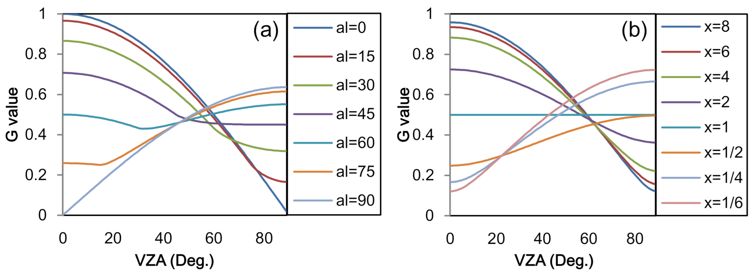
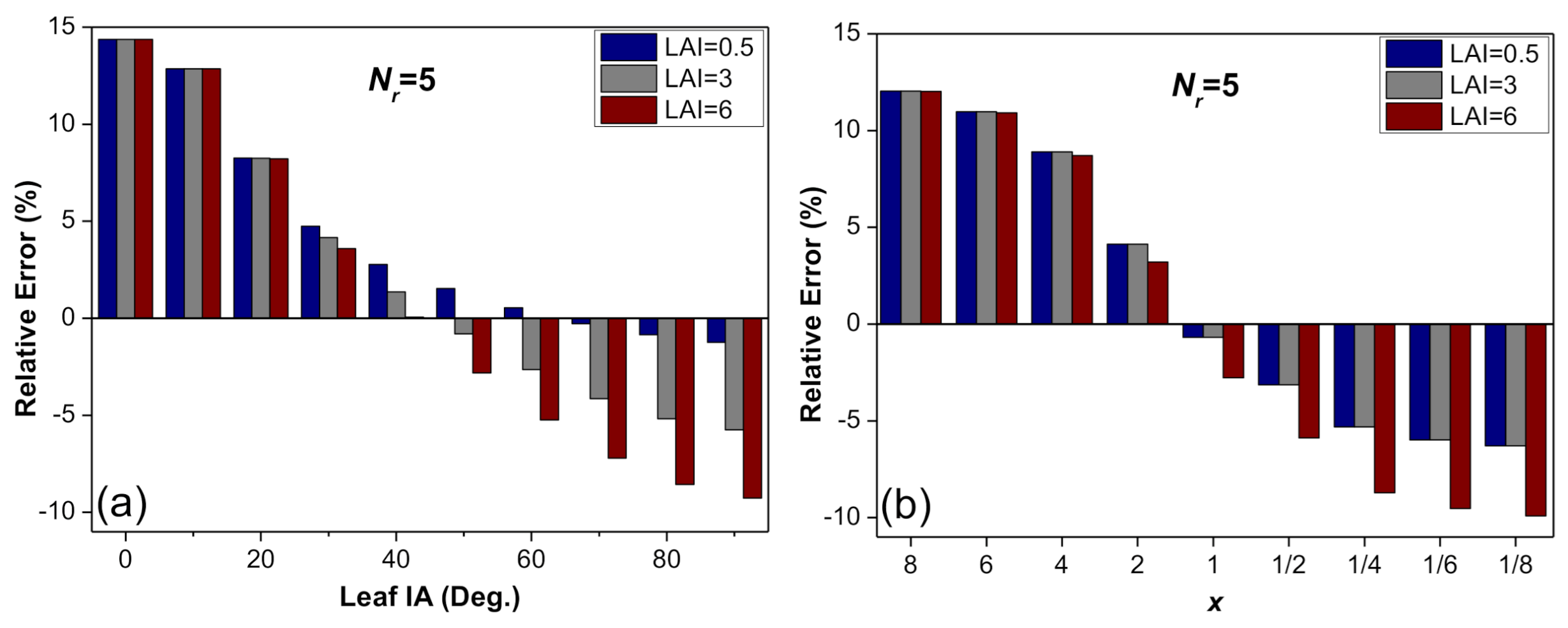
• Using (all) five PCA rings

Comparisons of $R_{error}$ among canopies with the different leaf IAs using all of the five PCA rings are shown in Figure 5. $R_{error}$ between $L_e^{L{i}_{cor}}$ and $L_e$ is closely related to the leaf IA. For horizontal and planophile leaf IA (such as leaf IA < 30° for the conical LAD (Figure 5a) or x > 2 for the ellipsoidal LAD (Figure 5b)), $L_e^{L{i}_{cor}}$ calculated by the discrete form of Miller’s equation is significantly larger than that calculated by Miller’s equation. $R_{error}$ is about 10% for the planophile leaf IA, meaning that $L_e$ is overestimated for the planophile leaf IAs although all five PCA rings are used. When the leaf IA is about 50° for the conical LAD or x is about 1 (spherical LAD) for the ellipsoidal LAD, $R_{error}$ can be ignored (lower than ±4%), meaning that the PCA has a good performance for these leaf IAs. With the increment of the leaf IA, $R_{error}$ is negative and $L_e$ is underestimated. The maximum can be up to −10%. In summary, $R_{error}$ increases as the leaf IAs deviate from the spherical LAD.

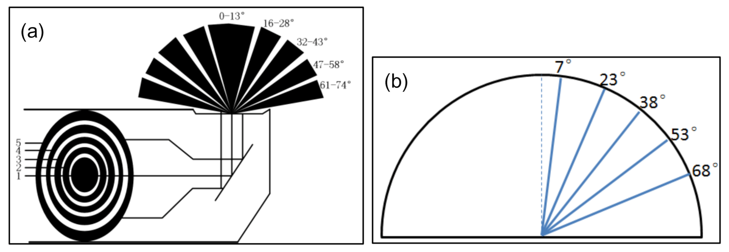
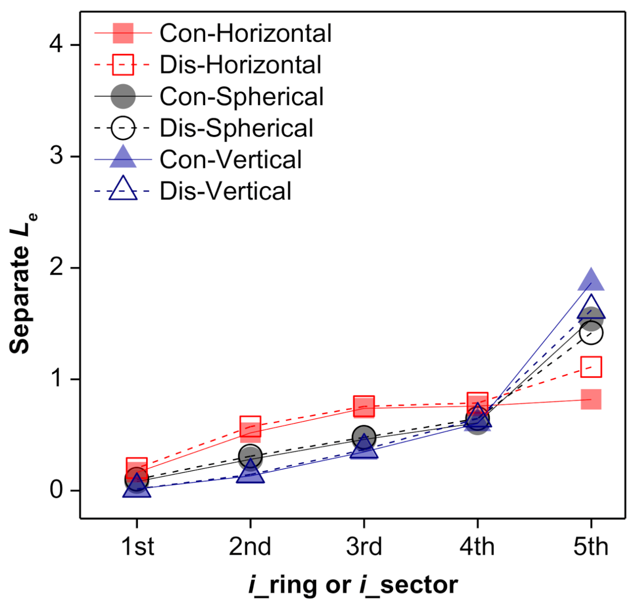
For further analysis, the whole hemispheric space (0−90°) was divided into five sectors corresponding to the right borders of the five rings of the PCA: 0−13°, 14−28°, 29−43°, 44−58°, and 59−90°, respectively. Thus, the five sectors corresponded to the five PCA rings. We separated the results of the definite integrals in Equation (3) according to the five sectors. Here, we noted the separated result in each sector as a separated $L_e$. Thus, each sector has a separated $L_e$ (noted as the separated $L_e^{Con}$), and the sum of separated $L_e^{Con}$ is $L_e$ in Equation (3). Similarly, we calculate the separated $L_e$ (noted as the separated $L_e^{Dis}$) in Equations (4) and (16) according to the PCA rings, and the sum of separated $L_e^{Dis}$ is $L_e^{L{i}_{cor}}$ in Equations (3) and (16). Taking LAI = 3 as an example, the separated $L_e^{Con}$ in each sector and $L_e^{Dis}$ in each PCA ring are compared to find the specific error (Figure 6).

The separated $L_e^{Dis}$ (dashed lines in Figure 6; prefix “Dis” in the legend) in the non-last (i.e., the first four) rings are almost close to the separated $L_e^{Con}$, indicating that there is no obvious error in the non-last rings, although the VZA ranges between the sectors and PCA rings are different. The separated $L_e^{Dis}$ in the non-last PCA rings are slightly overestimated. This is because the weight coefficients (w_j in Equation (4)) of the first four PCA rings are slightly larger than the corresponding continuous item of ($\sin \theta \mathrm{d}\theta$). For example, the first w_j (0.034) in Equation (4) is slightly larger than the corresponding item ($\sin \theta \mathrm{d}\theta$, approximately 0.032) in Equation (3). This means that the errors produced by the discrete VZAs are slight in the non-last PCA rings.

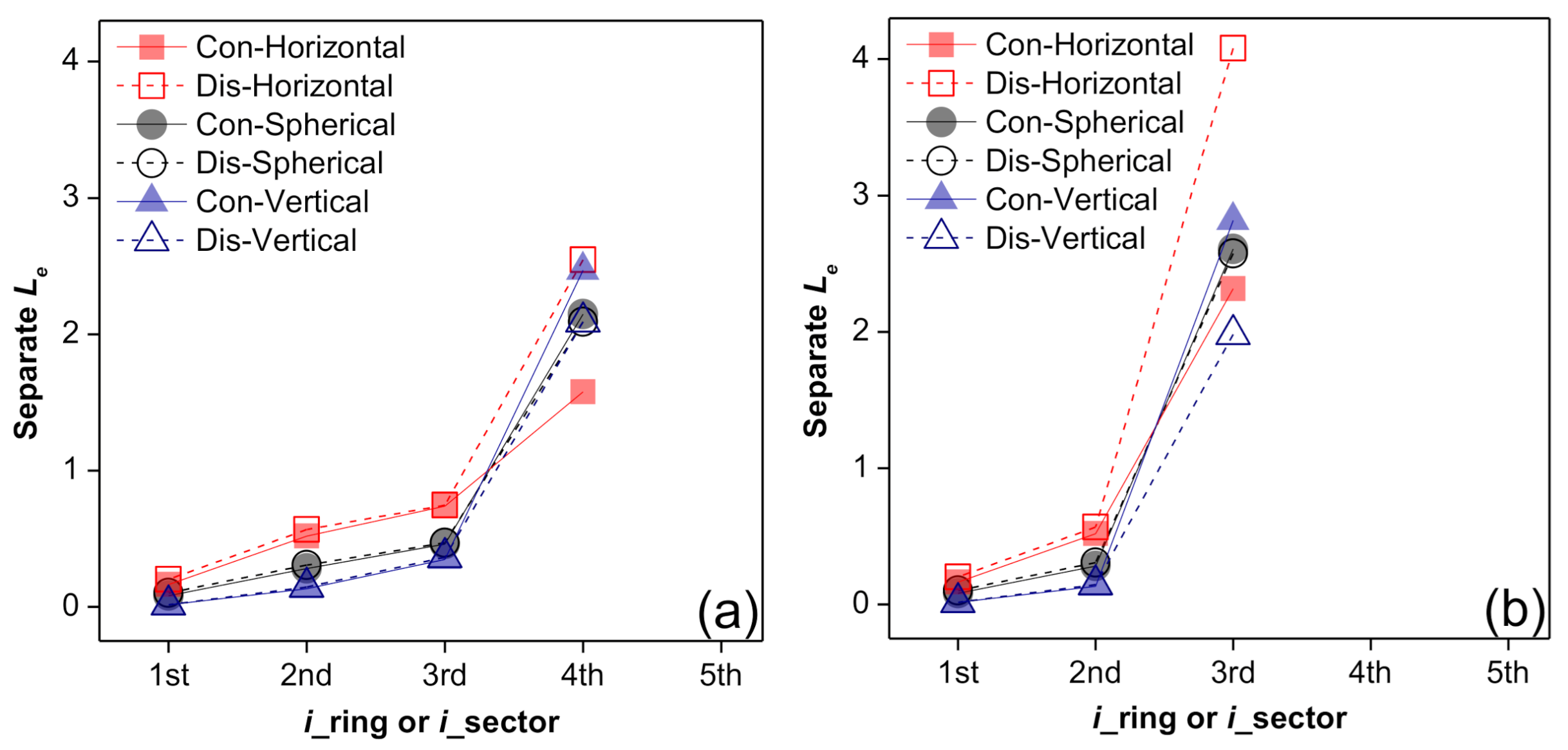
The main error exists in the last PCA ring. For canopies with a spherical leaf IA, the separated $L_e^{Dis}$ in the last PCA ring is slightly underestimated. Then, the difference between $L_e^{Dis}$ in the last PCA ring and $L_e^{Con}$ in the last sector can be offset by the first four sectors or PCA rings, thus, the total $L_e^{Dis}$ (sum of all separated $L_e^{Dis}$) is nearly equal to the total $L_e^{Con}$ (sum of all separated $L_e^{Con}$). However, for the horizontal and planophile leaf IAs, the separated $L_e^{Dis}$ in the last PCA ring is obviously overestimated compared with the separated $L_e^{Con}$; thus, the total $L_e^{Dis}$ is significantly overestimated. For the vertical and erectophile canopies, the separated $L_e^{Dis}$ in the last PCA ring is obviously underestimated; thus, the total $L_e^{Dis}$ is underestimated. Considering that the separated $L_e^{Dis}$ in the non-last PCA rings are slightly overestimated, the magnitude of errors for these types of leaf IA are smaller than those for the horizontal and planophile leaf IAs.

b.

Using four and three PCA rings

Fewer PCA rings inevitably leads to a higher degree of discretization of VZAs in the PCA, which must affect $L_e$ measured with the PCA. Here, all of the canopy parameters (except for the number of PCA rings) and the analysis method of $R_{error}$ are the same as those noted in the previous section. Comparison of $R_{\mathrm{error}}$ in $L_e$ measured with the PCA among canopies with the different leaf IAs using four and three PCA rings are shown in Figure 7. Notably, the scope of the vertical coordinates in Figure 7 is different from that in Figure 5, in order to achieve a more beautiful visualization.

The general change trends of the results in Figure 7 are similar to those in Figure 5. However, nearly all $R_{error}$ values in Figure 7 increase obviously with the decreasing number of PCA rings (except in the case of canopies in which the leaf IA is about 50° or a spherical LAD). For the horizontal leaf IA, $R_{error}$ can reach up to 35% and 60% with four and three PCA rings, respectively. For the erectophile leaf IA, the PCA results can be underestimated by 15% and 27% with four and three PCA rings, respectively. Even for the leaf IA = 40° or 60°, $R_{error}$ is also obvious when the number of PCA rings decreases to three: the $R_{error}$ can reach up to 23% and −15% for canopies with the leaf IA = 40° and 60°, respectively. The above phenomenon is due to the error of $L_e^{Dis}$ in the last PCA ring. Taking LAI = 3 as an example, the separated $L_e^{Dis}$ in the last ring is overestimated by about 66% and 100% for the horizontal leaf IA using four and three PCA rings, respectively (Figure 8).

In summary, decreasing the number of PCA rings can enhance the degree of discrete VZAs, and enlarge the magnitude of PCA error, especially for the planophile and erectophile leaf IAs.

3.2. Corrections

The above results show that the error produced by the discrete VZAs is closely related to the leaf IA. Thus, the correction for the error must be related to the leaf IA. In practice, leaf IA is often influenced by many environmental factors, such as wind and sunlight. Therefore, it is often a variable value and is not easily measured in situ. Moreover, the accurate measurement of leaf IA is in contradiction with the convenience of the PCA. Plant leaf IA type, which is an estimation of leaf IA, is often stable in a certain period of time. Here, we divided the whole hemispherical space equally into three sectors. Then, the leaf IAs were divided into three types: planophile (VZA: 0–30°), spherical-like (30–60°), and erectophile (60–90°). Linear relationships are used to correct the error produced by the discrete VZAs according to the three leaf IA types. Two corrections were made: (1) correction for only the last PCA ring (the “CL” method) and (2) the direct correction for total $L_e$ measured with the PCA (the “CT” method).

• “CL” method

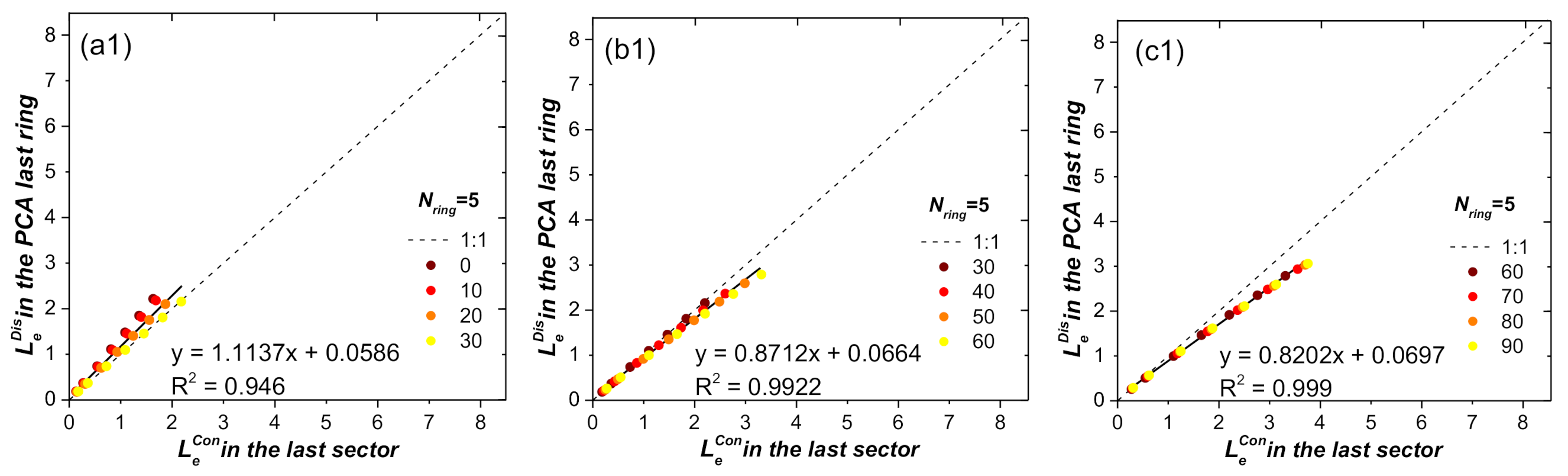
From the previous section, the default or original weight coefficients in the PCA rings are suitable for the spherical LAD, whereas they produce an error and need to be modified for other leaf IA types. The error of $L_e$ in the last PCA ring is mainly due to the use of incorrect weight coefficients for the last PCA ring. Here, we use the regression coefficients in Figure 9 to correct the original weight coefficients in the last PCA ring.

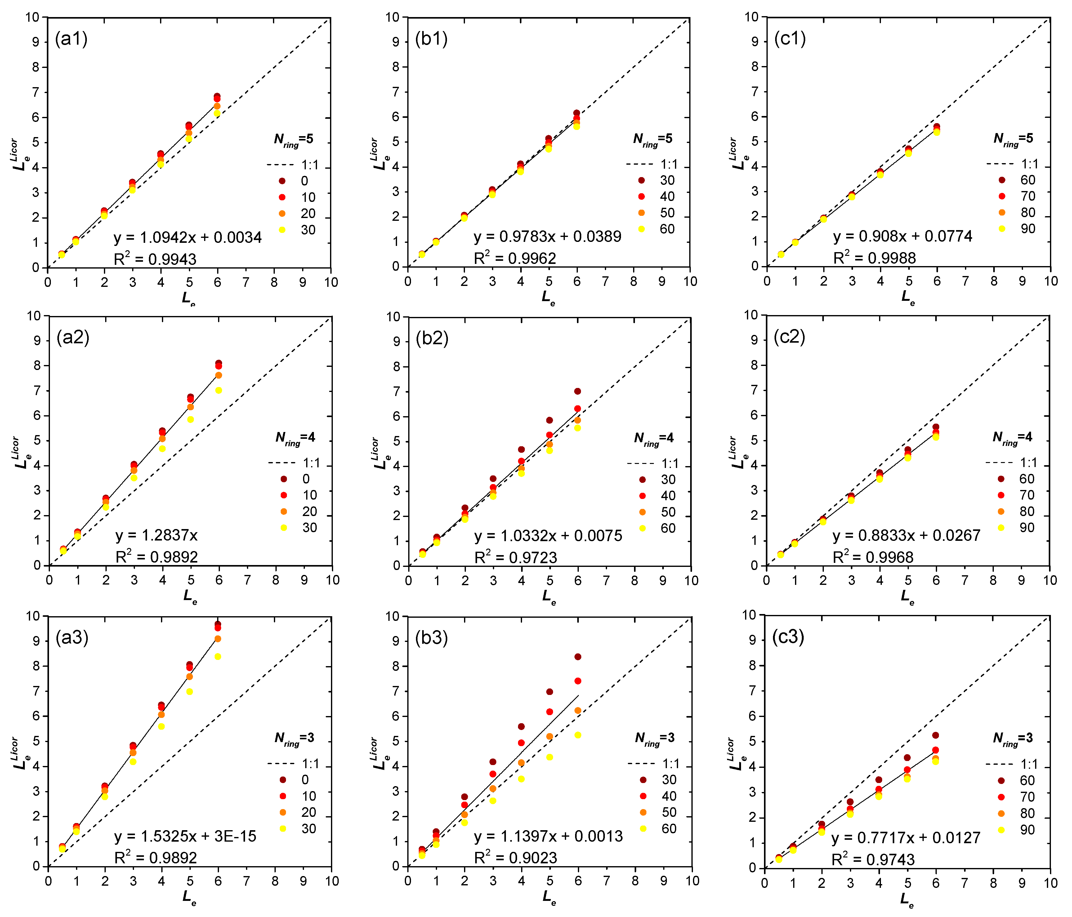
The linear relationships of the separated $L_e$ in the last PCA ring between the discrete ($L_e^{Dis}$) and continuous results ($L_e^{Con}$) are shown in Figure 9 with the three different leaf IA types (Figure 9a planophile, Figure 9b spherical-like, and Figure 9c erectophile) and with the decrement of the number of PCA rings from five to three (Figure 9(a1,b1,c1) five rings, Figure 9(a2,b2,c2) four rings, and Figure 9(a3,b3,c3) three rings). From Figure 9, the regression coefficients between $L_e^{Dis}$ in the last PCA ring and $L_e^{Con}$ in the last sector are closely related to the leaf IA types: all of the slopes of the regression line are larger than 1 for the planophile type, but lower than 1 for the erectophile type; the regression lines for the spherical-like types are around the 1:1 line. With the decrement of the number of PCA rings, the regression lines are generally distinct from the 1:1 line. With the exception of Figure 9(b3), all of the coefficients of determination (R²) are larger than 0.94, indicating that the correction is reasonable and acceptable. The scattering points in Figure 9 are concentrated around the regression lines (except for Figure 9(b3)), indicating that the magnitude of $L_e$ has little effect on the regression coefficients in most situations.

As nearly all of the values for R² in Figure 9 are close to 1, we provide the new weight coefficients for the last PCA ring (

Table 3. New weight coefficients of the PCA rings after the “CL” correction.

Number of PCA Rings	Leaf IA Type	Ring_1	Ring_2	Ring_3	Ring_4	Ring_5
5	Default *	0.034	0.104	0.160	0.218	0.494
	Planophile	0.034	0.104	0.160	0.218	0.444
	Spherical-like	0.034	0.104	0.160	0.218	0.567
	Erectophile	0.034	0.104	0.160	0.218	0.602
4	Default *	0.034	0.103	0.158	0.705	-
	Planophile	0.034	0.103	0.158	0.488	-
	Spherical-like	0.034	0.103	0.158	0.715	-
	Erectophile	0.034	0.104	0.160	0.831	-
3	Default *	0.034	0.103	0.863	-	-
	Planophile	0.034	0.103	0.525	-	-
	Spherical-like	0.034	0.103	0.769	-	-
	Erectophile	0.034	0.103	1.155	-	-

* “Default” means the default or original weight coefficients of the PCA.

) according to the regression coefficients in Figure 9. The only change for the new weight coefficients is the value in the last PCA ring. Generally, the values of the weight coefficients in the PCA last ring increase for the planophile type of leaf IA, but decrease for the erectophile type of leaf IA, according to Figure 9, and change slightly for the spherical-like type of leaf IA.

In summary, the correction for each specific leaf IA is not completely necessary although the error produced by the discrete VZAs is closely related to the specific leaf IA (Figure 6 and Figure 8).

b.

“CT” method

The relationships of total $L_e$ between the discrete ($L_e^{L{i}_{cor}}$, sum of the separated $L_e^{Dis}$ in all used PCA rings) and continuous result ($L_e$, sum of the separated $L_e^{Con}$ in all used sectors) are shown in Figure 10 with various leaf IA types (Figure 10a planophile, Figure 10b spherical-like, and Figure 10c erectophile) and with the decrement in the number of PCA rings from five to three (Figure 10(a1–c1) five rings, Figure 10(a2–c2) four rings, and Figure 10(a3–c3) three rings).

All of the R² of the relationships in Figure 10 are larger than 0.9, indicating that the relationships between $L_e^{L{i}_{cor}}$ and $L_e$ are also close, although we used the leaf IA type instead of the leaf IA. The regression coefficients are related to the leaf IA type and number of PCA rings, whereas the magnitude of $L_e$ has little effect on the regression coefficients in most situations in Figure 10. The planophile and erectophile types show a similar trend with the results in Figure 9: $L_e$ is underestimated with the PCA for the planophile-type canopies (all relationship slopes are lower than 1) but overestimated for the erectophile-type (all relationship slopes are larger than 1). $L_e$ is estimated well for the spherical-like type with five and four PCA rings. Nonetheless, with the decrement in the number of PCA rings, the relationship slopes are different from 1 (about 1.14 in Figure 10(b3)), indicating that the correction for the PCA is also needed; that is, the discrete VZA correction for the PCA is essential in most cases, especially for the planophile- and erectophile-type with four and three PCA rings.

3.3. Experiments

Planophile is a common type of leaf IA in many heliophile vegetables, such as green pepper, tomato, and soybean, when water and sunlight are sufficient. Erectophile is another common type of leaf IA in the early stage of many continuous canopies, such as rice, wheat, and some herbage.

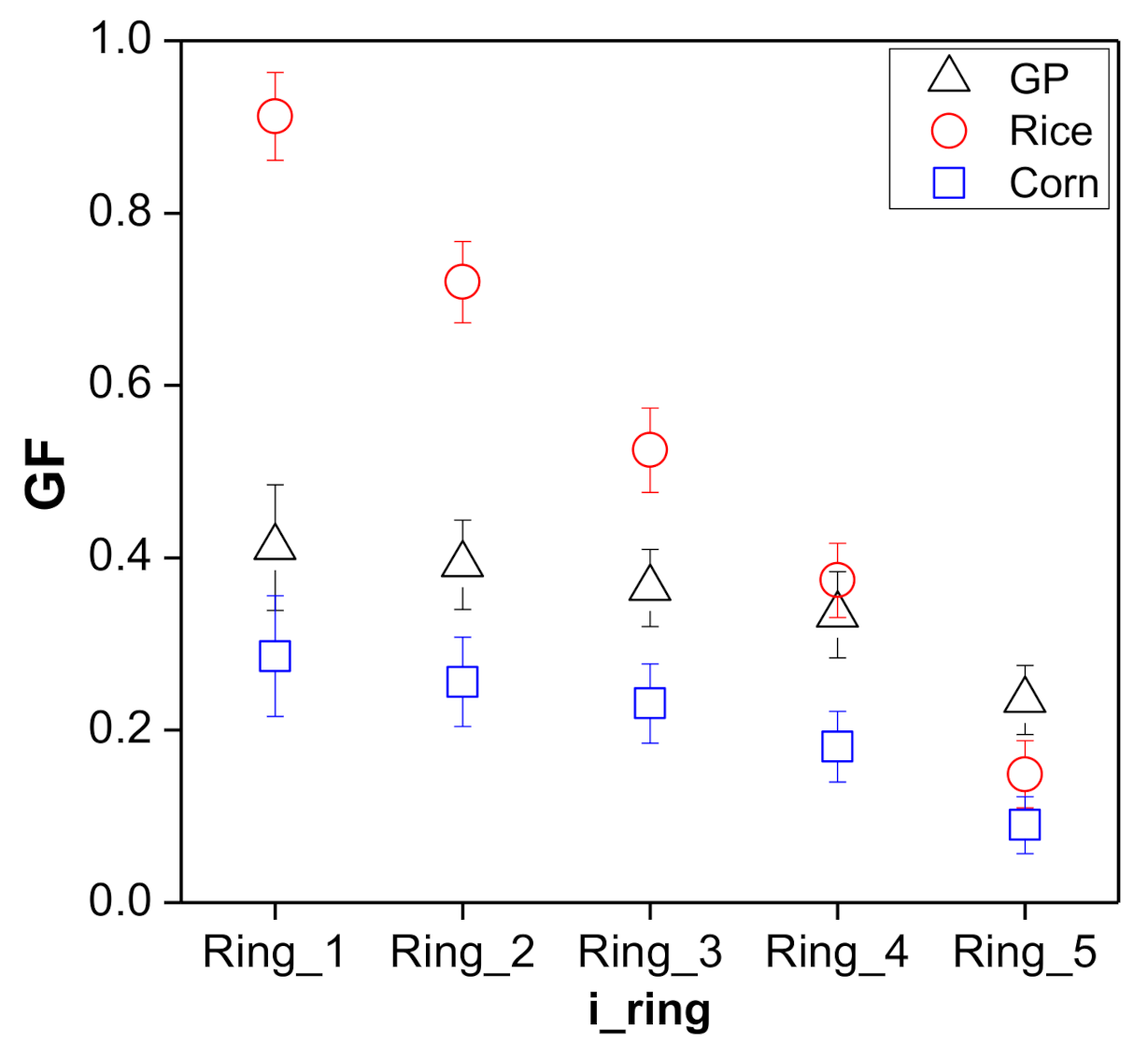
Three crop plots—a green pepper (GP) plot (E 32°20′47″; N 117°15′15″), a corn plot (E 32°20′28″; N 117°15′03″), and a rice plot (E 32°20′53″; N 117°15′02″) —were selected to validate the influence of discrete VZAs on the PCA. Experiments were conducted during July 1–3, 2018. All of the selected plants were in early stage to avoid the influence of fruits on the interception of light in the lens. The sizes of the three plots were 30× 30 m and there were five replicates initially. A view restrictor of 270° of the PCA was used in all plots to avoid the influence of the observer. As the IAs of dead leaves on the plants were distributed irregularly, they were needed to be removed. The LAI was measured by destructive sampling. The leaf IAs were measured using a protractor and a gradienter, and are listed in

Table 4. Leaf IA measurement of the three plots.

Plant	Minimum (°)	Maximum (°)	Mean (°)	Type
GP	4	20	10	Planophile
Corn	41	60	48	Spherical-like
Rice	68	89	82	Erectophile

. There were significant differences in leaf IA among the three plots: the leaf IA types of the three crops obviously belonged to planophile, spherical-like, and erectophile, respectively. The GFs were measured using the LAI-2000 PCA in an overcast situation (Figure 11). Finally, L_e in each plot was calculated in the FV2000 software (Li-Cor, Inc., Lincoln, NE) for the PCA (noted as L_e) using five, four, and three rings (noted as L_e__P5, L_e__P4, and L_e__P3, respectively,

Table 5. In situ measurement of L_e with the PCA and LAI in the three plots.

Plant	Leaf IA type	LAI	L5	L4	L3
GP	Planophile	1.15	1.29	1.41	1.61
Corn	Spherical-like	2.01	2.05	2.16	2.34
Rice	Erectophile	1.20	1.10	1.01	0.89

L₅ means L_e measured with five PCA rings; L₄ means L_e measured with four rings; L₃ means L_e measured with three rings.

). $R_{error}$ is used to describe the relative error between L_e measured with the PCA and the LAI (Figure 12).

L_e measured with the different numbers of PCA rings in the three plots are listed in Table 5. As there were no fruits and no obvious stalks in each of the three plots, foliage was the main object intercepting light. The influence of the discrete VZAs on the PCA in the three plots is similar to the results shown in Figure 5 and Figure 7. L_e measured with the PCA in the GP plot is larger than the true LAI, meaning that L_e is overestimated in the GP plot; on the contrary, the L_e in the rice plot is lower than the LAI, meaning L_e is overestimated in the plot. L_e measured with the PCA is closer to the true LAI in the corn plot than that in the other two plots (all $R_{error}$ of L_e in the corn plot are lower than those in the other two plots). This means that the PCA has higher performance in the corn plot than in the other two plots. Moreover, the gap between the value of L_e and LAI increased with the decrement of the number of PCA rings. For example, the value of L_e increased from 1.29 to 1.61 with the decrement of the number of PCA rings from five to three in the GP plot. Thus, the $R_{error}$ between L_e and LAI increased from 12.5% to 40.0% in the GP plot. Although in the corn plot with the spherical-like type of leaf IA, $R_{error}$ can reach up to about 15%. The different performance of the PCA in the three plots validates the theoretical deduction presented in Section 2.2.

L_e corrections were made for the three crop plots using the two methods: “CL” and “CT”. (1) We changed the weight coefficients (w_j) of the last PCA ring according to Table 3. Then, L_e was recalculated according to the new w_j in each plot (L_e is corrected as “L_{e _CL}” in Figure 12). 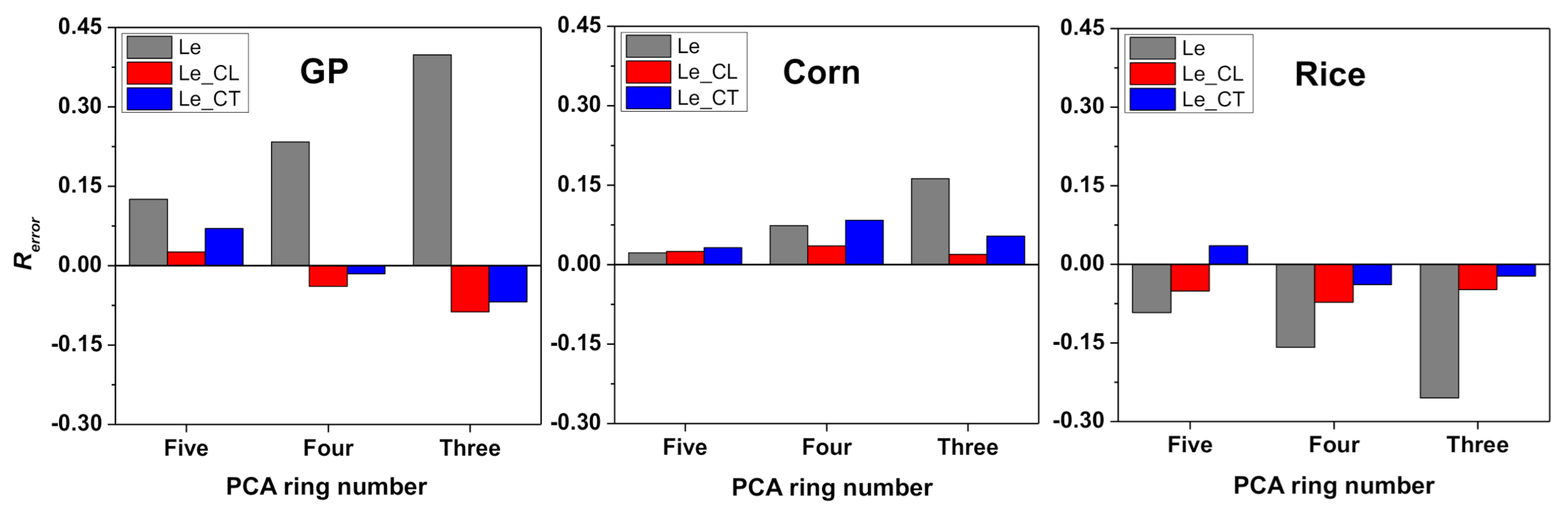(2) We directly recalculated L_e according to the linear regression coefficients in Figure 10 (L_e is corrected as “L_{e _CT}” in Figure 12). After correction, both the L_{e _CL} and L_{e _CT} are obviously closer to the LAI than L_e measured with the PCA in all three plots (all $R_{error}$ in the three plots are lower than 10%). In particular, with four and three rings, L_e errors produced by the discrete VZAs decrease significantly. This means that both of the two correction methods are effective for decreasing the error produced by the discrete VZAs.

The improvement due to the correction for L_e in the corn plot is not as clear as that in the other two plots (e.g., $R_{error}$ increases using five and four PCA rings after the “CT” correction method), although $R_{error}$ of L_e in the corn plot is not obvious (the largest $R_{error}$ is lower than 10%) after correction. This is due to the fact that the L_e error produced by the discrete VZAs can be neglected for the leaf IA ≈ 50° or the LAD meeting the spherical distribution (as shown in Figure 5 and Figure 7). In addition, the correction performed here is an approximation because corrected for L_e according to the three leaf IA types but not the specific leaf IAs. Therefore, the correction for the PCA with five or four rings is not necessary for the leaf IA ≈ 50° or the LAD meeting the spherical distribution.

4. Discussion

As the PCA has been widely used to estimate the effective leaf area index (L_e) indirectly in vegetation canopies, and to validate the retrieval LAI using remote sensing technique during the past 30 years, the series of studies using the PCA is an important topic [13,21,26,36]. This study proved and supported the previous preliminary results. Here, several aspects need to be discussed.

4.1. Error Produced by the Discrete VZAs

Miller’s equation as used in the PCA is the discrete form because only several rings are used, although the VZAs cover nearly all of the hemispherical space. Moreover, the large rings of PCA have often been suggested to be reduced in in situ L_e measurement by previous studies. Leblanc and Chen suggested that multiple scattering could increase the incident light into the PCA sensor, especially in the fifth ring [29]. Therefore, the effect of multiple scattering on the fifth ring of the PCA can lead to overestimation of the GF and underestimation of the L_e. Similarly, the effect of sunlight and the specular reflection [13] on the fifth ring of PCA can also lead to overestimating the GF and underestimating L_e. Additionally, the number of PCA rings needs to be reduced when the plot is not large enough to cover the whole range of the fifth PCA ring and there is contamination outside the plot [31]. A similar operation using the fewer PCA rings was suggested by Eckrich et al. [35]. It is commonly accepted that discrete or limited VZAs in the PCA may produce uncertainty because insufficient VZAs are used compared to the whole hemispherical space [10]. The study definitely proves why the error can be produced by the discrete VZAs and quantifies the magnitude of the error, especially when using a lower number of PCA rings.

The influence of discrete or limited VZAs is not merely a problem with the PCA; it is a common problem for many optical instruments. Digital hemispherical photographs (DHPs), which have a wider VZA range than the PCA (usually covering the whole hemispherical space), also have similar problems. In practice, the GFs at the large VZAs are too small to be classified in the photographs. Therefore, the values of GF at large VZAs are often equal to zero in the photographs. According to Equation (3), if the GF is equal to zero, L_e is equal to infinity. Therefore, the GFs at large VZAs cannot be used in Miller’s equation. In this situation, the wide VZAs in the DHPs also need to be reduced and the weight coefficients in the last VZAs cannot be calculated by 1 minus the sum of the weight coefficients in the front VZAs. The weight coefficients in each VZA need to be recalculated, similar to the approach used in this study before using Miller’s equation for the DHPs.

The influence of the discrete VZAs on the PCA is not merely a problem with the weight coefficients in the last PCA ring. In fact, there are two discrete components in Equations (3) and (4): the GF and the weight coefficient. The GF is actually an averaged value in each PCA ring. For example, the GF in the first ring is an average of the GF at the VZAs ranging from 0 to 13°. Therefore, only five averaged GFs can be measured by the PCA, although the PCA VZAs cover nearly the whole hemispherical space. From the results in this study (Figure 6 and Figure 8), the difference between the separated $L_e^{Con}$ and $L_e^{Dis}$ in the non-last ring can be ignored, regardless of what the leaf IA is, indicating that the influence of the average GF on the PCA is slight and can be neglected, although the average GF is an estimation from Equation (3) to Equation (4).

4.2. Leaf IAs Effect

One of the most important contributions of the Miller’s equation is the establishment of the relationship between L_e and the GF at the hemispherical VZAs without considering the specific leaf IA or the G value. Thus, the essence of Miller’s equation is that L_e can be measured using the GF at the hemispherical VZAs while neglecting the specific leaf IA. While, interestingly, although the leaf IA type cannot influence L_e calculated using Miller’s equation in hemispheric space, it may affect L_e measured with the PCA using the discrete form of Miller’s equation at several discrete VZAs in this study. This must be considered in LAI measurement with the PCA. The influence of leaf IA on the PCA was discussed by Stenberg et al. [31]. They noted that the error of L_e measured with the PCA may be due to non-spherical shoot orientation; as a result, the discrete form of Miller’s equations was no longer applicable. This study proved and supported the previous preliminary results. Moreover, the specific influence of various leaf IAs on L_e was quantitatively analyzed in detail in this study: L_e can be overestimated for the planophile type of leaf IA and underestimated for the erectophile type. The corrections according to the leaf IA types are effective means of reducing the error produced by the discrete VZAs.

4.3. Corrections

Two corrections were undertaken for the separated L_e or the weight coefficients of the last PCA ring (the “CL” method) and the total L_e measured with the PCA (the “CT” method) in this study. It is suggested that the “CL” method be used to correct for the error produced by the discrete VZAs, although the coefficients of determination in Figure 10 are generally larger than those in Figure 9. This is because the “CL” method is specifically used to correct for the error produced by the discrete VZAs. In practice, the PCA may not only be influenced by the discrete VZAs, but also by other factors (such as multiple scattering) in in situ L_e measurement. Therefore, using the “CT” correction for L_e measured with the PCA may not be appropriate. The “CT” method can be adopted in relatively ideal situations, such as when the sky is overcast. As the in situ measurement of L_e with the PCA may be affected by synthetic factors (for example, concurrently affected by non-photosynthesis components, multiple scattering, clumping effect, and foliage specular reflection), the “CL” correction for the discrete VZAs in this study can be used to solve the synthesis problem.

4.4. Discrete Canopies

Why and how the discrete VZAs affect L_e measured with the PCA for continuous canopies (such as crops and grasses) were clearly proven and shown in this study, respectively. For discrete canopies (such as forests), this influence also exists. Moreover, Equations (4–6) in Section 2.2 need to be added to the clumping index [36,37]. Therefore, both $G\left(\theta \right)$ and the clumping index can affect L_e measured with the PCA for discrete canopies. Similar to the case of $G\left(\theta \right)$ in Section 2.2, the variation of the product of $G\left(\theta \right)$ and the clumping index with the VZAs should be made clear. Although the clumping index has been reported to increase with VZAs in some forests [38,39], it has also been reported to decrease with VZAs in other scenes [36]. Considering the complex architecture of discrete canopies, the effect of the discrete VZAs for discrete canopies on the PCA is complicated. Our next work will investigate the relationship between the clumping index and VZAs, and then determine the influence of discrete VZAs on L_e measured with the PCA for discrete canopies.

5. Conclusions

In this study, why and how discrete VZAs may affect L_e measured with the PCA for continuous canopies were firstly proven and presented, respectively. A theoretical deduction is presented to prove why the discrete VZAs can affect L_e measured with the PCA: both the weight coefficient of the last PCA ring and the foliage G value are two main reasons. The magnitudes of the errors produced by the discrete VZAs are shown in detail. Specifically: (1) L_e measured with the PCA is overestimated for the planophile type of leaf IA and underestimated for the erectophile type; and (2) the influence can be amplified, or the relative error can increase with the increment of discretization or the decrement of the number of PCA rings. We recommend that the PCA is highly suitable for canopies with the spherical-like type of leaf IA. The leaf IA type needs to be considered and the “CL” correction for the error is suggested to be used when measuring L_e with the PCA, especially for planophile or erectophile types of leaf IA using four or fewer PCA rings.

References

1. Chen, J.M.; Black, T.A. Defining leaf area index for non-flat leaves. Plant Cell Environ. 1992, 15, 421–429. [Google Scholar] [CrossRef]
2. Myneni, R.B.; Hoffman, S.; Knyazikhin, Y.; Privette, J.L.; Glassy, J.; Tian, Y.; Wang, Y.; Song, X.; Zhang, Y.; Smith, G.R.; et al. Global products of vegetation leaf area and fraction absorbed PAR from year one of MODIS data. Remote Sens. Environ. 2002, 83, 214–231. [Google Scholar] [CrossRef] [Green Version]
3. Yin, G.; Cao, B.; Li, J.; Fan, W.; Zeng, Y.; Xu, B.; Zhao, W. Path Length Correction for Improving Leaf Area Index Measurements Over Sloping Terrains: A Deep Analysis Through Computer Simulation. IEEE Trans. Geosci. Remote Sens. 2020, 58, 4573–4589. [Google Scholar] [CrossRef]
4. Maki, M.; Sekiguchi, K.; Homma, K.; Hirooka, Y.; Oki, K. Estimation of rice yield by SIMRIW-RS, a model that integrates remote sensing data into a crop growth model. J. Agric. Meteorol. 2017, 73, 2–8. [Google Scholar] [CrossRef] [Green Version]
5. Breda, N.J.J. Ground-based measurements of leaf area index: A review of methods, instruments and current controversies. J. Exp. Bot. 2003, 54, 2403–2417. [Google Scholar] [CrossRef]
6. Zheng, G.; Moskal, L.M. Retrieving Leaf Area Index (LAI) Using Remote Sensing: Theories, Methods and Sensors. Sensors 2009, 9, 2719–2745. [Google Scholar] [CrossRef] [Green Version]
7. Chen, J.M.; Rich, P.M.; Gower, S.T.; Norman, J.M.; Plummer, S. Leaf area index of boreal forests: Theory, techniques, and measurements. J. Geophys. Res. Atmos. 1997, 102, 29429–29443. [Google Scholar] [CrossRef]
8. Yan, G.; Hu, R.; Luo, J.; Weiss, M.; Jiang, H.; Mu, X.; Xie, D.; Zhang, W. Review of indirect optical measurements of leaf area index: Recent advances, challenges, and perspectives. Agric. For. Meteorol. 2019, 265, 390–411. [Google Scholar] [CrossRef]
9. Hu, R.; Yan, G.; Mu, X.; Luo, J. Indirect measurement of leaf area index on the basis of path length distribution. Remote Sens. Environ. 2014, 155, 239–247. [Google Scholar] [CrossRef]
10. Weiss, M.; Baret, F.; Smith, G.J.; Jonckheere, I.; Coppin, P. Review of methods for in situ leaf area index (LAI) determination Part II. Estimation of LAI, errors and sampling. Agric. For. Meteorol. 2004, 121, 37–53. [Google Scholar] [CrossRef]
11. Jonckheere, I.; Fleck, S.; Nackaerts, K.; Muys, B.; Coppin, P.; Weiss, M.; Baret, F. Review of methods for in situ leaf area index determination—Part I. Theories, sensors and hemispherical photography. Agric. For. Meteorol. 2004, 121, 19–35. [Google Scholar] [CrossRef]
12. Garrigues, S.; Shabanov, N.V.; Swanson, K.; Morisette, J.T.; Baret, F.; Myneni, R.B. Intercomparison and sensitivity analysis of Leaf Area Index retrievals from LAI-2000, AccuPAR, and digital hemispherical photography over croplands. Agric. For. Meteorol. 2008, 148, 1193–1209. [Google Scholar] [CrossRef] [Green Version]
13. Kuusk, A. Specular reflection in the signal of LAI-2000 plant canopy analyzer. Agric. For. Meteorol. 2016, 221, 242–247. [Google Scholar] [CrossRef]
14. Chianucci, F.; Macfarlane, C.; Pisek, J.; Cutini, A.; Casa, R. Estimation of foliage clumping from the LAI-2000 Plant Canopy Analyzer: Effect of view caps. Trees 2015, 29, 355–366. [Google Scholar] [CrossRef]
15. Majasalmi, T.; Rautiainen, M.; Stenberg, P.; Rita, H. Optimizing the sampling scheme for LAI-2000 measurements in a boreal forest. Agric. For. Meteorol. 2012, 154–155, 38–43. [Google Scholar] [CrossRef]
16. Arias, D.; Calvo-Alvarado, J.; Dohrenbusch, A. Calibration of LAI-2000 to estimate leaf area index (LAI) and assessment of its relationship with stand productivity in six native and introduced tree species in Costa Rica. For. Ecol. Manag. 2007, 247, 185–193. [Google Scholar] [CrossRef]
17. Dovey, S.B.; du Toit, B. Calibration of LAI-2000 canopy analyser with leaf area index in a young eucalypt stand. Trees 2006, 20, 273–277. [Google Scholar] [CrossRef]
18. Stenberg, P. Correcting LAI-2000 estimates for the clumping of needles in shoots of conifers. Agric. For. Meteorol. 1996, 79, 1–8. [Google Scholar] [CrossRef]
19. Smith, N.J.; Chen, J.M.; Black, T.A. Effects of clumping on estimates of stand leaf area index using the LI-COR LAI-2000. Can. J. Forest Res. 1993, 23, 1940–1943. [Google Scholar] [CrossRef]
20. Zheng, G.; Ma, L.; Eitel, J.U.H.; He, W.; Magney, T.S.; Moskal, L.M.; Li, M. Retrieving Directional Gap Fraction, Extinction Coefficient, and Effective Leaf Area Index by Incorporating Scan Angle Information From Discrete Aerial Lidar Data. IEEE Trans. Geosci. Remote Sens. 2017, 55, 577–590. [Google Scholar] [CrossRef]
21. Kuusk, A.; Pisek, J.; Lang, M.; Märdla, S. Estimation of Gap Fraction and Foliage Clumping in Forest Canopies. Remote Sens. Basel. 2018, 10, 1153. [Google Scholar] [CrossRef] [Green Version]
22. Lang, A.; Yueqin, X. Estimation of leaf area index from transmission of direct sunlight in discontinuous canopies. Agric. For. Meteorol. 1986, 37, 229–243. [Google Scholar] [CrossRef]
23. Lang, A. Leaf-area and average leaf angle from transmission of direct sunlight. Aust. J. Bot. 1986, 34, 349–355. [Google Scholar] [CrossRef]
24. Woodgate, W.; Armston, J.D.; Disney, M.; Jones, S.D.; Suarez, L.; Hill, M.J.; Wilkes, P.; Soto-Berelov, M. Quantifying the impact of woody material on leaf area index estimation from hemispherical photography using 3D canopy simulations. Agric. For. Meteorol. 2016, 226–227, 1–12. [Google Scholar] [CrossRef]
25. Zou, J.; Zhuang, Y.; Chianucci, F.; Mai, C.; Lin, W.; Leng, P.; Luo, S.; Yan, B. Comparison of Seven Inversion Models for Estimating Plant and Woody Area Indices of Leaf-on and Leaf-off Forest Canopy Using Explicit 3D Forest Scenes. Remote Sens. Basel 2018, 10, 1297. [Google Scholar] [CrossRef] [Green Version]
26. Zou, J.; Leng, P.; Hou, W.; Zhong, P.; Chen, L.; Mai, C.; Qian, Y.; Zuo, Y. Evaluating Two Optical Methods of Woody-to-Total Area Ratio with Destructive Measurements at Five Larix gmelinii Rupr. Forest Plots in China. Forests 2018, 9, 746. [Google Scholar] [CrossRef] [Green Version]
27. Nackaerts, K.; Coppin, P.; Muys, B.; Hermy, M. Sampling methodology for LAI measurements with LAI-2000 in small forest stands. Agric. For. Meteorol. 2000, 101, 247–250. [Google Scholar] [CrossRef]
28. Villalobos, F.J.; Orgaz, F.; Mateos, L. Non-destructive measurement of leaf area in olive (Olea europaea L.) trees using a gap inversion method. Agric. For. Meteorol. 1995, 73, 29–42. [Google Scholar] [CrossRef]
29. Leblanc, S.G.; Chen, J.M. A practical scheme for correcting multiple scattering effects on optical LAI measurements. Agric. For. Meteorol. 2001, 110, 125–139. [Google Scholar] [CrossRef]
30. Pearse, G.D.; Watt, M.S.; Morgenroth, J. Comparison of optical LAI measurements under diffuse and clear skies after correcting for scattered radiation. Agric. For. Meteorol. 2016, 221, 61–70. [Google Scholar] [CrossRef]
31. Stenberg, P.; Linder, S.; Smolander, H.; Flower-Ellis, J. Performance of the LAI-2000 plant canopy analyzer in estimating leaf area index of some Scots pine stands. Tree Physiol. 1994, 14, 981–995. [Google Scholar] [CrossRef]
32. Miller, J.B. A formula for average foliage density. Aust. J. Bot. 1967, 15, 141–144. [Google Scholar] [CrossRef]
33. Varhola, A.; Coops, N.C. Estimation of watershed-level distributed forest structure metrics relevant to hydrologic modeling using LiDAR and Landsat. J. Hydrol. 2013, 487, 70–86. [Google Scholar] [CrossRef]
34. Majasalmi, T.; Korhonen, L.; Korpela, I.; Vauhkonen, J. Application of 3D triangulations of airborne laser scanning data to estimate boreal forest leaf area index. Int. J. Appl. Earth Obs. 2017, 59, 53–62. [Google Scholar] [CrossRef]
35. Eckrich, C.A.; Flaherty, E.A.; Ben-David, M. Estimating Leaf Area Index in Southeast Alaska: A Comparison of Two Techniques. PLoS ONE 2013, 8, e77642. [Google Scholar]
36. Geng, J.; Chen, J.; Tu, L.; Tian, Q.; Wang, L.; Yang, R.; Yang, Y.; Huang, Y.; Fan, W.; Lv, C.; et al. Influence of the exclusion distance among trees on gap fraction and foliage clumping index of forest plantations. Trees 2016, 30, 1683–1693. [Google Scholar] [CrossRef]
37. Gonsamo, A.; Pellikka, P. The computation of foliage clumping index using hemispherical photography. Agric. For. Meteorol. 2009, 149, 1781–1787. [Google Scholar] [CrossRef]
38. Leblanc, S.G.; Chen, J.M.; Fernandes, R.; Deering, D.W.; Conley, A. Methodology comparison for canopy structure parameters extraction from digital hemispherical photography in boreal forests. Agric. For. Meteorol. 2005, 129, 187–207. [Google Scholar] [CrossRef] [Green Version]
39. Pisek, J.; Lang, M.; Nilson, T.; Korhonen, L.; Karu, H. Comparison of methods for measuring gap size distribution and canopy nonrandomness at Järvselja RAMI (RAdiation transfer Model Intercomparison) test sites. Agric. For. Meteorol. 2011, 151, 365–377. [Google Scholar] [CrossRef]
Figure 1. Yearly published items about indirect LAI measurement. (The search was conducted on December 12, 2019, using Web of Science with the keyword combination TOPIC: [“LAI-2000” OR “LAI2000” OR “LAI-2200” OR “LAI2200” OR “plant canopy analyzer”)] AND TOPIC: [“digital hemispherical photography” OR “fisheye photography” OR “hemispherical photography”] AND TOPIC: (Lidar AND LAI) AND TOPIC: (TRAC AND LAI) AND TOPIC: [“AccuPAR” OR “LP-80”].).
Remotesensing 13 01405 g001
Figure 2. Total number of published items regarding the five main LAI measuring instruments from 1992 to 2019.
Remotesensing 13 01405 g002
Figure 3. Five concentric rings of the LAI-2000 or LAI-2200 plant canopy analyzer (PCA) ((a) the five concentric rings in the PCA (Li-Cor, Inc., Lincoln, NE); (b) blue lines indicate the middle view zenith angles (VZAs) in the PCA rings).
Remotesensing 13 01405 g003
Figure 4. Different characteristics of G values at various VZAs. (a) Conic distribution. “al” in the legend represents the leaf inclination angle (IA) (degree). (b) Ellipsoidal distribution. “x “in the legend represents x in Equation (15), x = 1 is the spherical distribution.
Remotesensing 13 01405 g004
Figure 5. Comparison of R e r r o r caused by the discrete VZAs in the PCA between canopies with different leaf IAs using the five PCA rings. (a) Conical leaf angle distribution (LAD). (b) Ellipsoidal LAD. “Nr is the number of rings being used. “x” in the subplot (b) represents x in Equation (15).
Remotesensing 13 01405 g005
Figure 6. Comparison of the separated L e calculated by Miller’s equation (prefix “Con” means L e Con in the legend) and the discrete form of Miller’s equation using the five PCA rings (prefix “Dis” means L e D i s ) for canopies with different leaf IAs. “i_ring” means the serial number of the PCA ring; “i_sector” means the serial number of the sector.
Remotesensing 13 01405 g006
Figure 7. Comparison of R error produced by the discrete VZAs among canopies with the different leaf IAs using four (a,b) and three (c,d) rings. (a,c) Canopies with the conical LAD. (b,d) Canopies with the ellipsoidal LAD. “Nr” represents the number of PCA rings. “x” in subplot (b,d) represents x in Equation (15). Notably, the scope of vertical coordinates here is different from that in Figure 5 for beautiful visualization).
Remotesensing 13 01405 g007
Figure 8. Comparison of the separated L e calculated using Miller’s equation (prefix “Con” means L e Con in legend) and the discrete form of Miller’s equation using (a) four and (b) three PCA rings (prefix “Dis” means L e D i s ) for canopies with different leaf IAs. “i_ring” means the serial number of the PCA rings.“i_sector” means the serial number of the sector.
Remotesensing 13 01405 g008
Figure 9. The relationship between the separated L e D i s in the last PCA ring and the separated L e C o n in the last sector. (a to c) represent Le measurement using the five, four, and three PCA rings, respectively. (1 to 3) represent the three different leaf IA types: planophile, spherical-like, and erectophile, respectively. Values in the legend refer to the leaf IAs (degree).
Remotesensing 13 01405 g009aRemotesensing 13 01405 g009b
Figure 10. The relationships of L e between the discrete and continuous results. (a to c) represent Le measurement using the five, four, and three PCA rings, respectively. (1 to 3) represent the three different leaf IA types: planophile, spherical-like, and erectophile, respectively. Values in the legend mean leaf IAs (degree).
Remotesensing 13 01405 g010
Figure 11. In situ measurement of the gap fraction (GF) with the PCA in the three plots.
Remotesensing 13 01405 g011
Figure 12. Correction for Le using the two methods (“Le_CL” means Le corrected by the “CL” method; “Le_CT” means Le corrected by the “CT” method) in the three plots.
Remotesensing 13 01405 g012