
Estimating Plant Nitrogen Concentration of Rice through Fusing Vegetation Indices and Color Moments Derived from UAV-RGB Images


Abstract
:
1. Introduction
2. Materials and Methods
2.1. Experiment Design
2.2. Data Collection
2.2.1. Determination of PNC
2.2.2. Image Acquisition
2.3. Image Data Processing
2.3.1. Image Mosaic
2.3.2. Calculation of VIs

| Data type | Variables | Equation/Description | Reference |
|---|---|---|---|
| RGB-VIs | NRI | R/(R+G+B) | [33] |
| NGI | G/(R+G+B) | [33] | |
| NBI | B/(R+G+B) | [33] | |
| G/R | G/R | [34] | |
| G/B | G/B | [34] | |
| R/B | R/B | [34] | |
| ExR | (1.4R-G)/(G+R+B) | [35] | |
| ExG | (2*G-R-B) /(G+R+B) | [36] | |
| GMR | G-R | [17] | |
| INT | (R+G+B)/3 | [37] | |
| VARI | (G-R)/(G+R-B) | [38] | |
| NGRDI | (G-R)/(G+R) | [13] | |
| Color moments | H | The average of hue | [27] |
| H_var | The variance of hue | [27] | |
| H_ske | The skewness of hue | [27] | |
| S | The average of saturation | [27] | |
| S_var | The variance of saturation | [27] | |
| S_ske | The skewness of saturation | [27] | |
| V | The average of value | [27] | |
| V_var | The variance of value | [27] | |
| V_ske | The skewness of value | [27] |
2.3.3. Calculation of Color Moments
2.4. Algorithms of Multivariate Regression Model
2.4.1. PLSR
2.4.2. Random Forests
2.5. Statistical Analysis
3. Results
3.1. Descriptive Analysis of Measured PNC Data
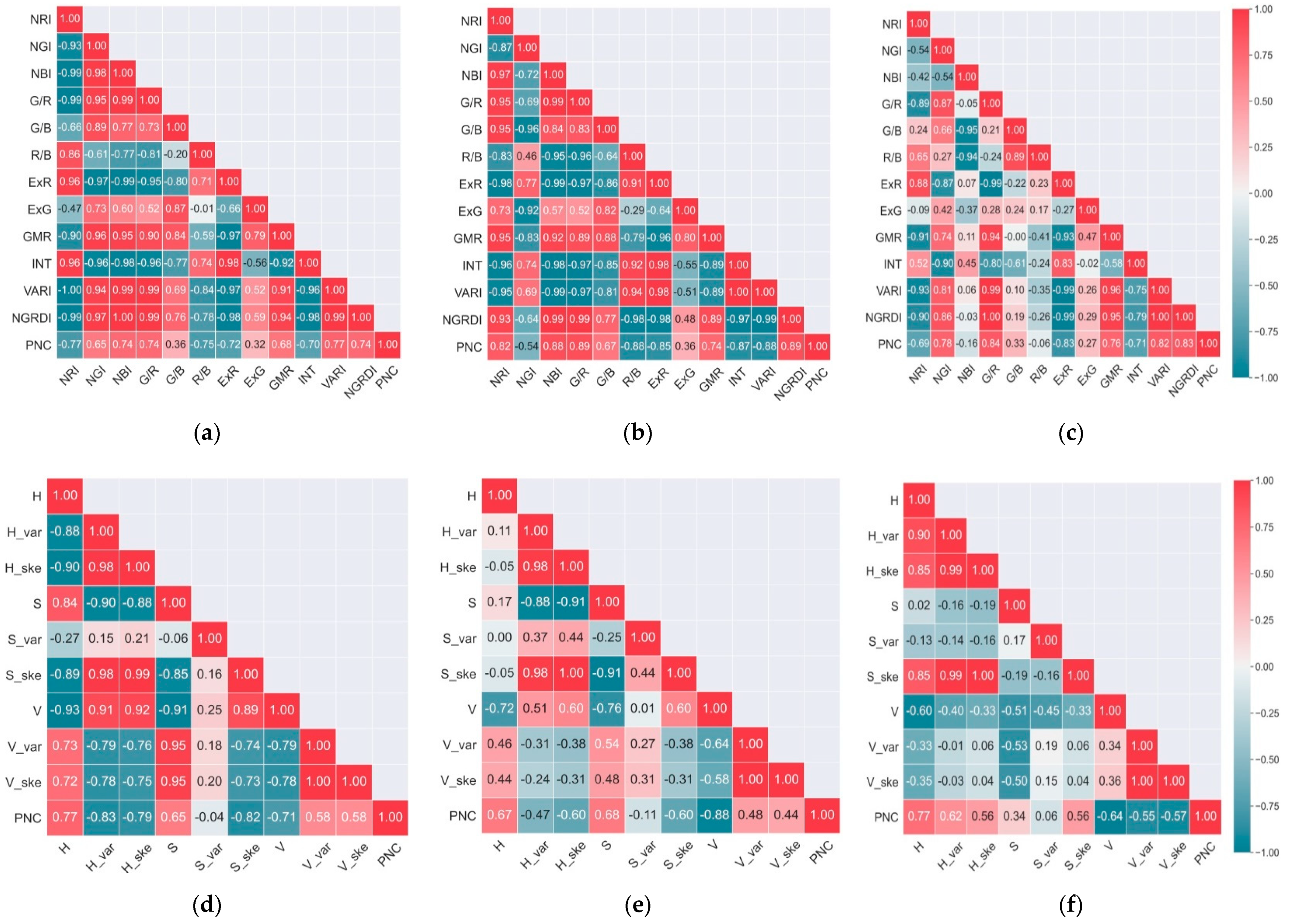
3.2. Correlations between RGB-VIs, Color Moments and PNC
3.3. PLSR Analysis
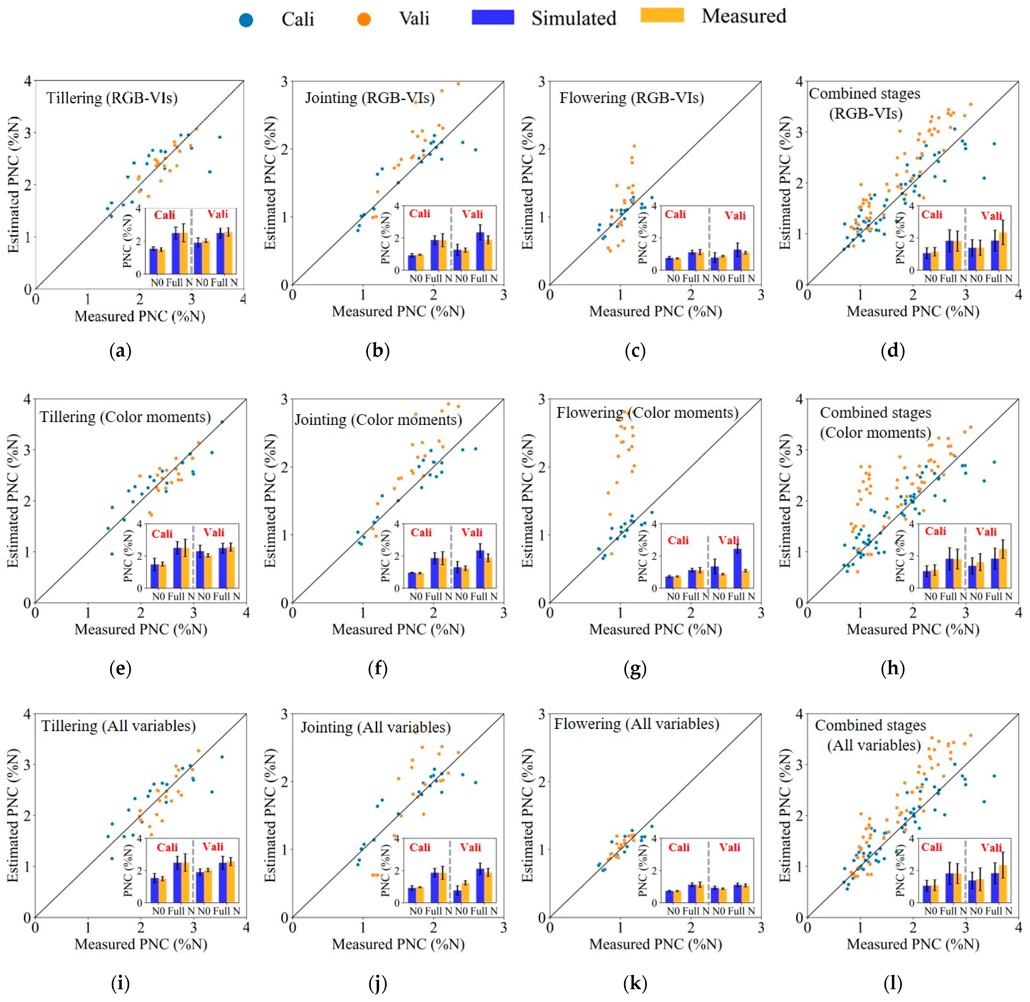
3.4. RF Analysis
4. Discussion
4.1. Comparisons of the PLSR and RF Models
4.2. Fusion of RGB-VIs and Color Moments for PNC Estimation
4.3. Implications of UAV-Based RGB Imagery for Crop Monitoring
5. Conclusions
Author Contributions
Funding
Data Availability Statement
Acknowledgments
Conflicts of Interest
References
- Cantrell, R.P. The Rice Genome: The Cereal of the World’s Poor Takes Center Stage. Science 2002, 296, 53. [Google Scholar] [CrossRef] [PubMed]
- Huang, S.; Miao, Y.; Zhao, G.; Yuan, F.; Ma, X.; Tan, C.; Yu, W.; Gnyp, M.L.; Lenz-Wiedemann, V.I.; Rascher, U.; et al. Satellite Remote Sensing-Based In-Season Diagnosis of Rice Nitrogen Status in Northeast China. Remote Sens. 2015, 7, 10646–10667. [Google Scholar] [CrossRef] [Green Version]
- Zheng, H.; Cheng, T.; Li, D.; Yao, X.; Tian, Y.; Cao, W.; Zhu, Y. Combining Unmanned Aerial Vehicle (UAV)-Based Multispectral Imagery and Ground-Based Hyperspectral Data for Plant Nitrogen Concentration Estimation in Rice. Front. Plant Sci. 2018, 9. [Google Scholar] [CrossRef]
- Zheng, H.; Ma, J.; Zhou, M.; Li, D.; Yao, X.; Cao, W.; Zhu, Y.; Cheng, T. Enhancing the Nitrogen Signals of Rice Canopies across Critical Growth Stages through the Integration of Textural and Spectral Information from Unmanned Aerial Vehicle (UAV) Multispectral Imagery. Remote Sens. 2020, 12, 957. [Google Scholar] [CrossRef] [Green Version]
- Padilla, F.M.; Peña-Fleitas, M.T.; Gallardo, M.; Thompson, R.B. Evaluation of optical sensor measurements of canopy reflectance and of leaf flavonols and chlorophyll contents to assess crop nitrogen status of muskmelon. Eur. J. Agron. 2014, 58, 39–52. [Google Scholar] [CrossRef]
- Miphokasap, P.; Honda, K.; Vaiphasa, C.; Souris, M.; Nagai, M. Estimating Canopy Nitrogen Concentration in Sugarcane Using Field Imaging Spectroscopy. Remote Sens. 2012, 4, 1651–1670. [Google Scholar] [CrossRef] [Green Version]
- Tian, Y.; Yao, X.; Yang, J.; Cao, W.; Hannaway, D.; Zhu, Y. Assessing newly developed and published vegetation indices for estimating rice leaf nitrogen concentration with ground- and space-based hyperspectral reflectance. Field Crop. Res. 2011, 120, 299–310. [Google Scholar] [CrossRef]
- Wang, W.; Yao, X.; Yao, X.; Tian, Y.; Liu, X.; Ni, J.; Cao, W.; Zhu, Y. Estimating leaf nitrogen concentration with three-band vegetation indices in rice and wheat. Field Crop. Res. 2012, 129, 90–98. [Google Scholar] [CrossRef]
- Kalacska, M.; Lalonde, M.; Moore, T. Estimation of foliar chlorophyll and nitrogen content in an ombrotrophic bog from hyperspectral data: Scaling from leaf to image. Remote Sens. Environ. 2015, 169, 270–279. [Google Scholar] [CrossRef]
- Lepine, L.C.; Ollinger, S.V.; Ouimette, A.P.; Martin, M.E. Examining spectral reflectance features related to foliar nitrogen in forests: Implications for broad-scale nitrogen mapping. Remote Sens. Environ. 2016, 173, 174–186. [Google Scholar] [CrossRef]
- Crema, A.; Boschetti, M.; Nutini, F.; Cillis, D.; Casa, R. Influence of Soil Properties on Maize and Wheat Nitrogen Status Assessment from Sentinel-2 Data. Remote Sens. 2020, 12, 2175. [Google Scholar] [CrossRef]
- Loozen, Y.; Rebel, K.T.; de Jong, S.M.; Lu, M.; Ollinger, S.V.; Wassen, M.J.; Karssenberg, D. Mapping canopy nitrogen in European forests using remote sensing and environmental variables with the random forests method. Remote Sens. Environ. 2020, 247, 111933. [Google Scholar] [CrossRef]
- Li, Y.; Chen, D.; Walker, C.; Angus, J. Estimating the nitrogen status of crops using a digital camera. Field Crop. Res. 2010, 118, 221–227. [Google Scholar] [CrossRef]
- Bendig, J.; Yu, K.; Aasen, H.; Bolten, A.; Bennertz, S.; Broscheit, J.; Gnyp, M.L.; Bareth, G. Combining UAV-based plant height from crop surface models, visible, and near infrared vegetation indices for biomass monitoring in barley. Int. J. Appl. Earth Obs. Geoinf. 2015, 39, 79–87. [Google Scholar] [CrossRef]
- Yang, G.; Liu, J.; Zhao, C.; Li, Z.; Huang, Y.; Yu, H.; Xu, B.; Yang, X.; Zhu, D.; Zhang, X.; et al. Unmanned Aerial Vehicle Remote Sensing for Field-Based Crop Phenotyping: Current Status and Perspectives. Front. Plant Sci. 2017, 8, 1111. [Google Scholar] [CrossRef]
- Sidike, P.; Sagan, V.; Qumsiyeh, M.; Maimaitijiang, M.; Essa, A.; Asari, V. Adaptive Trigonometric Transformation Function with Image Contrast and Color Enhancement: Application to Unmanned Aerial System Imagery. IEEE Geosci. Remote Sens. Lett. 2018, 15, 404–408. [Google Scholar] [CrossRef]
- Wang, Y.; Wang, D.; Zhang, G.; Wang, J. Estimating nitrogen status of rice using the image segmentation of G-R thresholding method. Field Crop. Res. 2013, 149, 33–39. [Google Scholar] [CrossRef]
- Babel, M.; Agarwal, A.; Swain, D.; Herath, S. Evaluation of climate change impacts and adaptation measures for rice cultivation in Northeast Thailand. Clim. Res. 2011, 46, 137–146. [Google Scholar] [CrossRef] [Green Version]
- Fanourakis, D.; Briese, C.; Max, J.F.; Kleinen, S.; Putz, A.; Fiorani, F.; Ulbrich, A.; Schurr, U. Rapid determination of leaf area and plant height by using light curtain arrays in four species with contrasting shoot architecture. Plant Methods 2014, 10, 9. [Google Scholar] [CrossRef] [Green Version]
- Golzarian, M.R.; Frick, R.A.; Rajendran, K.; Berger, B.; Roy, S.; Tester, M.; Lun, D.S. Accurate inference of shoot biomass from high-throughput images of cereal plants. Plant Methods 2011, 7, 2. [Google Scholar] [CrossRef] [Green Version]
- Bendig, J.; Bolten, A.; Bennertz, S.; Broscheit, J.; Eichfuss, S.; Bareth, G. Estimating Biomass of Barley Using Crop Surface Models (CSMs) Derived from UAV-Based RGB Imaging. Remote Sens. 2014, 6, 10395–10412. [Google Scholar] [CrossRef] [Green Version]
- Jiang, J.; Cai, W.; Zheng, H.; Cheng, T.; Tian, Y.; Zhu, Y.; Ehsani, R.; Hu, Y.; Niu, Q.; Gui, L.; et al. Using Digital Cameras on an Unmanned Aerial Vehicle to Derive Optimum Color Vegetation Indices for Leaf Nitrogen Concentration Monitoring in Winter Wheat. Remote Sens. 2019, 11, 2667. [Google Scholar] [CrossRef] [Green Version]
- Fu, Y.; Yang, G.; Li, Z.; Song, X.; Li, Z.; Xu, X.; Wang, P.; Zhao, C. Winter Wheat Nitrogen Status Estimation Using UAV-Based RGB Imagery and Gaussian Processes Regression. Remote Sens. 2020, 12, 3778. [Google Scholar] [CrossRef]
- Rorie, R.L.; Purcell, L.C.; Mozaffari, M.; Karcher, D.E.; King, C.A.; Marsh, M.C.; Longer, D.E. Association of “Greenness” in Corn with Yield and Leaf Nitrogen Concentration. Agron. J. 2011, 103, 529–535. [Google Scholar] [CrossRef] [Green Version]
- Li, S.; Yuan, F.; Ata-Ui-Karim, S.T.; Zheng, H.; Cheng, T.; Liu, X.; Tian, Y.; Zhu, Y.; Cao, W.; Cao, Q. Combining Color Indices and Textures of UAV-Based Digital Imagery for Rice LAI Estimation. Remote Sens. 2019, 11, 1763. [Google Scholar] [CrossRef] [Green Version]
- Yue, J.; Yang, G.; Tian, Q.; Feng, H.; Xu, K.; Zhou, C. Estimate of winter-wheat above-ground biomass based on UAV ultrahigh-ground-resolution image textures and vegetation indices. ISPRS J. Photogramm. Remote Sens. 2019, 150, 226–244. [Google Scholar] [CrossRef]
- Stricker, M.A.; Orengo, M. Similarity of color images. In Proceedings of the Storage and Retrieval for Image and Video Databases III—International Society Optical Engineering, San Jose, CA, USA, 23 March 1995; pp. 381–392. [Google Scholar]
- Li, W.; Niu, Z.; Chen, H.; Li, D.; Wu, M.; Zhao, W. Remote estimation of canopy height and aboveground biomass of maize using high-resolution stereo images from a low-cost unmanned aerial vehicle system. Ecol. Indic. 2016, 67, 637–648. [Google Scholar] [CrossRef]
- Page, A.L.; Miller, R.H.; Keeney, D.R. Methods of Soil Analysis: Chemical and Microbiological Properties; American Society of Agronomy: Madison, WI, USA, 1982. [Google Scholar]
- Yu, N.; Li, L.; Schmitz, N.; Tian, L.F.; Greenberg, J.A.; Diers, B.W. Development of methods to improve soybean yield estimation and predict plant maturity with an unmanned aerial vehicle-based platform. Remote Sens. Environ. 2016, 187, 91–101. [Google Scholar] [CrossRef]
- Qiu, Z.; Xiang, H.; Ma, F.; Du, C. Qualifications of Rice Growth Indicators Optimized at Different Growth Stages Using Unmanned Aerial Vehicle Digital Imagery. Remote Sens. 2020, 12, 3228. [Google Scholar] [CrossRef]
- Saberioon, M.; Amin, M.; Anuar, A.; Gholizadeh, A.; Wayayok, A.; Khairunniza-Bejo, S. Assessment of rice leaf chlorophyll content using visible bands at different growth stages at both the leaf and canopy scale. Int. J. Appl. Earth Obs. Geoinf. 2014, 32, 35–45. [Google Scholar] [CrossRef]
- Liu, K.; Li, Y.; Han, T.; Yu, X.; Ye, H.; Hu, H.; Hu, Z. Evaluation of grain yield based on digital images of rice canopy. Plant Methods 2019, 15, 28. [Google Scholar] [CrossRef] [PubMed]
- Maimaitijiang, M.; Sagan, V.; Sidike, P.; Maimaitiyiming, M.; Hartling, S.; Peterson, K.T.; Maw, M.J.; Shakoor, N.; Mockler, T.; Fritschi, F.B. Vegetation Index Weighted Canopy Volume Model (CVMVI) for soybean biomass estimation from Unmanned Aerial System-based RGB imagery. ISPRS J. Photogramm. Remote Sens. 2019, 151, 27–41. [Google Scholar] [CrossRef]
- Meyer, G.E.; Neto, J.C. Verification of color vegetation indices for automated crop imaging applications. Comput. Electron. Agric. 2008, 63, 282–293. [Google Scholar] [CrossRef]
- Woebbecke, D.M.; Meyer, G.E.; Vonbargen, K.; Mortensen, D.A. Color Indexes for Weed Identification under Various Soil, Residue, and Lighting Conditions. Trans. Asae 1995, 38, 259–269. [Google Scholar] [CrossRef]
- Ahmad, I.S.; Reid, J.F. Evaluation of Colour Representations for Maize Images. J. Agric. Eng. Res. 1996, 63, 185–195. [Google Scholar] [CrossRef]
- Sakamoto, T.; Gitelson, A.A.; Wardlow, B.D.; Arkebauer, T.J.; Verma, S.B.; Suyker, A.E.; Shibayama, M. Application of day and night digital photographs for estimating maize biophysical characteristics. Precis. Agric. 2012, 13, 285–301. [Google Scholar] [CrossRef] [Green Version]
- Stricker, M.A.; Dimai, A. Color Indexing with Weak Spatial Constraints. In Proceedings of the IS&T/SPIE’s Symposium on Electronic Imaging: Science and Technology, San Jose, CA, USA, 13 March 1996; pp. 29–40. [Google Scholar]
- Grossman, Y.; Ustin, S.; Jacquemoud, S.; Sanderson, E.; Schmuck, G.; Verdebout, J. Critique of stepwise multiple linear regression for the extraction of leaf biochemistry information from leaf reflectance data. Remote Sens. Environ. 1996, 56, 182–193. [Google Scholar] [CrossRef]
- Fassio, A.; Cozzolino, D. Non-destructive prediction of chemical composition in sunflower seeds by near infrared spectroscopy. Ind. Crop. Prod. 2004, 20, 321–329. [Google Scholar] [CrossRef]
- Nguyen, H.T.; Lee, B.-W. Assessment of rice leaf growth and nitrogen status by hyperspectral canopy reflectance and partial least square regression. Eur. J. Agron. 2006, 24, 349–356. [Google Scholar] [CrossRef]
- Breiman, L. Random Forests. Mach. Learn. 2001, 45, 5–32. [Google Scholar] [CrossRef] [Green Version]
- Enciso, J.; Avila, C.A.; Jung, J.; Elsayed-Farag, S.; Chang, A.; Yeom, J.; Landivar, J.; Maeda, M.; Chavez, J.C. Validation of agronomic UAV and field measurements for tomato varieties. Comput. Electron. Agric. 2019, 158, 278–283. [Google Scholar] [CrossRef]
- Loague, K. The impact of land use on estimates of pesticide leaching potential: Assessments and uncertainties. J. Contam. Hydrol. 1991, 8, 157–175. [Google Scholar] [CrossRef]
- Plénet, D.; Lemaire, G. Relationships between dynamics of nitrogen uptake and dry matter accumulation in maize crops. Determination of critical N concentration. Plant Soil 1999, 216, 65–82. [Google Scholar] [CrossRef]
- Cutler, D.R.; Edwards, T.C., Jr.; Beard, K.H.; Cutler, A.; Hess, K.T.; Gibson, J.; Lawler, J.J. Random Forests for Classification in Ecology. Ecology 2007, 88, 2783–2792. [Google Scholar] [CrossRef] [PubMed]
- Maimaitijiang, M.; Sagan, V.; Sidike, P.; Daloye, A.M.; Erkbol, H.; Fritschi, F.B. Crop Monitoring Using Satellite/UAV Data Fusion and Machine Learning. Remote Sens. 2020, 12, 1357. [Google Scholar] [CrossRef]
- Osco, L.; Junior, J.; Ramos, A.; Furuya, D.; Santana, D.; Teodoro, L.; Gonçalves, W.; Baio, F.; Pistori, H.; Junior, C.; et al. Leaf Nitrogen Concentration and Plant Height Prediction for Maize Using UAV-Based Multispectral Imagery and Machine Learning Techniques. Remote Sens. 2020, 12, 3237. [Google Scholar] [CrossRef]
- Liang, L.; Di, L.; Huang, T.; Wang, J.; Lin, L.; Wang, L.; Yang, M. Estimation of Leaf Nitrogen Content in Wheat Using New Hyperspectral Indices and a Random Forest Regression Algorithm. Remote Sens. 2018, 10, 1940. [Google Scholar] [CrossRef] [Green Version]
- Stroppiana, D.; Boschetti, M.; Brivio, P.A.; Bocchi, S. Plant nitrogen concentration in paddy rice from field canopy hyperspectral radiometry. Field Crop. Res. 2009, 111, 119–129. [Google Scholar] [CrossRef]
- Prey, L.; Schmidhalter, U. Sensitivity of Vegetation Indices for Estimating Vegetative N Status in Winter Wheat. Sensors 2019, 19, 3712. [Google Scholar] [CrossRef] [Green Version]
- Yu, K.; Li, F.; Gnyp, M.L.; Miao, Y.; Bareth, G.; Chen, X. Remotely detecting canopy nitrogen concentration and uptake of paddy rice in the Northeast China Plain. ISPRS J. Photogramm. Remote Sens. 2013, 78, 102–115. [Google Scholar] [CrossRef]
- Maesano, M.; Khoury, S.; Nakhle, F.; Firrincieli, A.; Gay, A.; Tauro, F.; Harfouche, A. UAV-Based LiDAR for High-Throughput Determination of Plant Height and Above-Ground Biomass of the Bioenergy Grass Arundo donax. Remote Sens. 2020, 12, 3464. [Google Scholar] [CrossRef]
- Bareth, G.; Aasen, H.; Bendig, J.; Gnyp, M.L.; Bolten, A.; Jung, A.; Michels, R.; Soukkamaki, J. Low-weight and UAV-based Hyperspectral Full-frame Cameras for Monitoring Crops: Spectral Comparison with Portable Spectroradiometer Measurements. Photogramm. Fernerkund. Geoinf. 2015, 1, 69–79. [Google Scholar] [CrossRef]
- Kopačková-Strnadová, V.; Koucká, L.; Jelének, J.; Lhotáková, Z.; Oulehle, F. Canopy Top, Height and Photosynthetic Pigment Estimation Using Parrot Sequoia Multispectral Imagery and the Unmanned Aerial Vehicle (UAV). Remote Sens. 2021, 13, 705. [Google Scholar] [CrossRef]
- Poley, L.G.; McDermid, G.J. A Systematic Review of the Factors Influencing the Estimation of Vegetation Aboveground Biomass Using Unmanned Aerial Systems. Remote Sens. 2020, 12, 1052. [Google Scholar] [CrossRef] [Green Version]
- Zhang, J.; Wang, C.; Yang, C.; Jiang, Z.; Zhou, G.; Wang, B.; Shi, Y.; Zhang, D.; You, L.; Xie, J. Evaluation of a UAV-mounted consumer grade camera with different spectral modifications and two handheld spectral sensors for rapeseed growth monitoring: Performance and influencing factors. Precis. Agric. 2020, 21, 1092–1120. [Google Scholar] [CrossRef]
- Hasan, U.; Sawut, M.; Chen, S. Estimating the Leaf Area Index of Winter Wheat Based on Unmanned Aerial Vehicle RGB-Image Parameters. Sustainability 2019, 11, 6829. [Google Scholar] [CrossRef] [Green Version]
- Niu, Y.; Zhang, L.; Zhang, H.; Han, W.; Peng, X. Estimating Above-Ground Biomass of Maize Using Features Derived from UAV-Based RGB Imagery. Remote Sens. 2019, 11, 1261. [Google Scholar] [CrossRef] [Green Version]
- De Castro, A.I.; Torres-Sánchez, J.; Peña, J.M.; Jiménez-Brenes, F.M.; Csillik, O.; López-Granados, F. An Automatic Random Forest-OBIA Algorithm for Early Weed Mapping between and within Crop Rows Using UAV Imagery. Remote Sens. 2018, 10, 285. [Google Scholar] [CrossRef] [Green Version]
- Fu, Y.; Yang, G.; Song, X.; Li, Z.; Xu, X.; Feng, H.; Zhao, C. Improved Estimation of Winter Wheat Aboveground Biomass Using Multiscale Textures Extracted from UAV-Based Digital Images and Hyperspectral Feature Analysis. Remote Sens. 2021, 13, 581. [Google Scholar] [CrossRef]
- Modica, G.; Messina, G.; De Luca, G.; Fiozzo, V.; Praticò, S. Monitoring the vegetation vigor in heterogeneous citrus and olive orchards. A multiscale object-based approach to extract trees’ crowns from UAV multispectral imagery. Comput. Electron. Agric. 2020, 175, 105500. [Google Scholar] [CrossRef]
- Shahhosseini, M.; Hu, G.; Archontoulis, S.V. Forecasting Corn Yield with Machine Learning Ensembles. Front. Plant Sci. 2020, 11, 1120. [Google Scholar] [CrossRef] [PubMed]
- Cao, J.; Zhang, Z.; Tao, F.; Zhang, L.; Luo, Y.; Zhang, J.; Han, J.; Xie, J. Integrating Multi-Source Data for Rice Yield Prediction across China using Machine Learning and Deep Learning Approaches. Agric. For. Meteorol. 2021, 297, 108275. [Google Scholar] [CrossRef]
- Cao, J.; Zhang, Z.; Luo, Y.; Zhang, L.; Zhang, J.; Li, Z.; Tao, F. Wheat yield predictions at a county and field scale with deep learning, machine learning, and google earth engine. Eur. J. Agron. 2021, 123, 126204. [Google Scholar] [CrossRef]
- Yang, Q.; Shi, L.; Han, J.; Zha, Y.; Zhu, P. Deep convolutional neural networks for rice grain yield estimation at the ripening stage using UAV-based remotely sensed images. Field Crop. Res. 2019, 235, 142–153. [Google Scholar] [CrossRef]
- Yang, Q.; Shi, L.; Han, J.; Yu, J.; Huang, K. A near real-time deep learning approach for detecting rice phenology based on UAV images. Agric. For. Meteorol. 2020, 287, 107938. [Google Scholar] [CrossRef]


| Treatment | Cultivar | Fertilizer Rate (kg/ha) | ||
|---|---|---|---|---|
| N | P2O5 | K2O | ||
| N0 | Wuyunjing 23 (2018) Nanjing 5055 (2019) | 0 | 0 | 0 |
| N1 | 240 | 60 | 120 | |
| N2 | 240 (30%) 1 | 60 | 120 | |
| N3 | 240 (40%) 2 | 60 | 120 | |
| N4 | 240 (50%) 3 | 60 | 120 | |
| Year | UAV Flight Date | Sampling Date | Growth Stage |
|---|---|---|---|
| 2018 | 19 July | 19 July | Tillering |
| 11 August | 11 August | Jointing | |
| 9 September | 9 September | Flowering | |
| 2019 | 14 July | 14 July | Tillering |
| 12 August | 12 August | Jointing | |
| 8 September | 8 September | Flowering |
| Dataset | Stages | PNC (%N) | |||
|---|---|---|---|---|---|
| Min | Max | Mean | SD | ||
| Calibration (2019) | Tillering | 1.4 | 3.5 | 2.3 | 0.6 |
| Jointing | 0.9 | 2.6 | 1.7 | 0.5 | |
| Flowering | 0.7 | 1.4 | 1.1 | 0.2 | |
| Validation (2018) | Tillering | 2.0 | 3.1 | 2.5 | 0.3 |
| Jointing | 1.1 | 2.4 | 1.8 | 0.3 | |
| Flowering | 0.8 | 1.2 | 1.0 | 0.1 | |
| Stages | Dataset | Calibration | Validation | ||
|---|---|---|---|---|---|
| R2 | NRMSE | R2 | NRMSE | ||
| Tillering | RGB-VIs | 0.62 | 0.16 | 0.63 | 0.11 |
| Color moments | 0.72 | 0.14 | 0.32 | 0.12 | |
| All variables | 0.79 | 0.12 | 0.68 | 0.10 | |
| Jointing | RGB-VIs | 0.80 | 0.13 | 0.81 | 0.29 |
| Color moments | 0.89 | 0.10 | 0.80 | 0.28 | |
| All variables | 0.84 | 0.12 | 0.75 | 0.24 | |
| Flowering | RGB-VIs | 0.71 | 0.11 | 0.60 | 0.36 |
| Color moments | 0.75 | 0.10 | 0.33 | 1.22 | |
| All variables | 0.77 | 0.10 | 0.73 | 0.15 | |
| Combined stages | RGB-VIs | 0.80 | 0.19 | 0.84 | 0.30 |
| Color moments | 0.81 | 0.18 | 0.50 | 0.41 | |
| All variables | 0.83 | 0.17 | 0.87 | 0.29 | |
| Parameter | Description | Range | Stages | Model | ||
|---|---|---|---|---|---|---|
| RGB-VIs Only | Color Moments Only | All Variables | ||||
| max_depth | The maximum depth of the tree | 2−6 | Tillering | 2 | 3 | 6 |
| Jointing | 5 | 6 | 2 | |||
| Flowering | 6 | 2 | 2 | |||
| All | 6 | 6 | 4 | |||
| min_samples_split | The minimum number of samples required to split an internal node | 2−8 | Tillering | 2 | 4 | 2 |
| Jointing | 4 | 2 | 2 | |||
| Flowering | 4 | 4 | 4 | |||
| All | 2 | 2 | 2 | |||
| min_samples_leaf | The minimum number of samples required to be at a leaf node | 1−12 | Tillering | 4 | 8 | 4 |
| Jointing | 4 | 2 | 6 | |||
| Flowering | 4 | 2 | 8 | |||
| All | 6 | 4 | 2 | |||
| Model | Tillering | Jointing | Flowering | Combined Stages | ||||
|---|---|---|---|---|---|---|---|---|
| Variable | Importance | Variable | Importance | Variable | Importance | Variable | Importance | |
| RGB-VIs only | NRI | 0.160 | INT | 0.209 | ExR | 0.353 | NRI | 0.439 |
| GMR | 0.127 | ExR | 0.177 | NGRDI | 0.182 | VARI | 0.146 | |
| R/B | 0.126 | NGI | 0.145 | G/R | 0.113 | G/R | 0.104 | |
| INT | 0.120 | NRI | 0.136 | NGI | 0.108 | NGRDI | 0.097 | |
| NGRDI | 0.104 | VARI | 0.117 | INT | 0.092 | G/B | 0.067 | |
| Color moments only | H | 0.269 | V | 0.632 | H | 0.706 | V | 0.562 |
| V | 0.192 | S | 0.183 | H_var | 0.086 | H | 0.315 | |
| H_ske | 0.174 | H | 0.139 | S_ske | 0.081 | S_var | 0.025 | |
| H_var | 0.113 | S_ske | 0.025 | V | 0.032 | S_ske | 0.022 | |
| S_ske | 0.103 | V_var | 0.005 | H_ske | 0.032 | H_var | 0.019 | |
| All variables | H | 0.125 | ExR | 0.231 | ExR | 0.306 | NRI | 0.420 |
| R/B | 0.093 | G/R | 0.136 | NGRDI | 0.166 | G/R | 0.125 | |
| H_ske | 0.088 | NRI | 0.126 | G/R | 0.160 | VARI | 0.095 | |
| NRI | 0.085 | VARI | 0.099 | H_var | 0.101 | NGRDI | 0.066 | |
| H_var | 0.080 | V | 0.088 | NGI | 0.091 | V | 0.062 | |
| Stages | Dataset | Calibration | Validation | ||
|---|---|---|---|---|---|
| R2 | NRMSE | R2 | NRMSE | ||
| Tillering | RGB-VIs | 0.86 | 0.11 | 0.62 | 0.08 |
| Color moments | 0.73 | 0.15 | 0.57 | 0.08 | |
| All variables | 0.89 | 0.10 | 0.69 | 0.07 | |
| Jointing | RGB-VIs | 0.88 | 0.10 | 0.82 | 0.09 |
| Color moments | 0.90 | 0.10 | 0.75 | 0.10 | |
| All variables | 0.93 | 0.08 | 0.84 | 0.08 | |
| Flowering | RGB-VIs | 0.79 | 0.10 | 0.63 | 0.09 |
| Color moments | 0.73 | 0.11 | 0.59 | 0.11 | |
| All variables | 0.83 | 0.09 | 0.71 | 0.08 | |
| Combined stages | RGB-VIs | 0.93 | 0.19 | 0.89 | 0.15 |
| Color moments | 0.94 | 0.16 | 0.54 | 1.46 | |
| All variables | 0.95 | 0.15 | 0.91 | 0.13 | |
Publisher’s Note: MDPI stays neutral with regard to jurisdictional claims in published maps and institutional affiliations. |
© 2021 by the authors. Licensee MDPI, Basel, Switzerland. This article is an open access article distributed under the terms and conditions of the Creative Commons Attribution (CC BY) license (https://creativecommons.org/licenses/by/4.0/).
Share and Cite
Ge, H.; Xiang, H.; Ma, F.; Li, Z.; Qiu, Z.; Tan, Z.; Du, C. Estimating Plant Nitrogen Concentration of Rice through Fusing Vegetation Indices and Color Moments Derived from UAV-RGB Images. Remote Sens. 2021, 13, 1620. https://0-doi-org.brum.beds.ac.uk/10.3390/rs13091620
Ge H, Xiang H, Ma F, Li Z, Qiu Z, Tan Z, Du C. Estimating Plant Nitrogen Concentration of Rice through Fusing Vegetation Indices and Color Moments Derived from UAV-RGB Images. Remote Sensing. 2021; 13(9):1620. https://0-doi-org.brum.beds.ac.uk/10.3390/rs13091620
Chicago/Turabian StyleGe, Haixiao, Haitao Xiang, Fei Ma, Zhenwang Li, Zhengchao Qiu, Zhengzheng Tan, and Changwen Du. 2021. "Estimating Plant Nitrogen Concentration of Rice through Fusing Vegetation Indices and Color Moments Derived from UAV-RGB Images" Remote Sensing 13, no. 9: 1620. https://0-doi-org.brum.beds.ac.uk/10.3390/rs13091620