Article

Mapping Smallholder Maize Farms Using Multi-Temporal Sentinel-1 Data in Support of the Sustainable Development Goals

by
Zinhle Mashaba-Munghemezulu
1,2,*,
George Johannes Chirima
1,2 and
Cilence Munghemezulu
2
1
Department of Geography, Geoinformatics and Meteorology, University of Pretoria, Pretoria 0028, South Africa
2
Geoinformation Science Division, Agricultural Research Council Institute for Soil, Climate and Water, Pretoria 0001, South Africa
*
Author to whom correspondence should be addressed.
Submission received: 1 March 2021 / Revised: 30 March 2021 / Accepted: 6 April 2021 / Published: 24 April 2021

Abstract

:
Reducing food insecurity in developing countries is one of the crucial targets of the Sustainable Development Goals (SDGs). Smallholder farmers play a crucial role in combating food insecurity. However, local planning agencies and governments do not have adequate spatial information on smallholder farmers, and this affects the monitoring of the SDGs. This study utilized Sentinel-1 multi-temporal data to develop a framework for mapping smallholder maize farms and to estimate maize production area as a parameter for supporting the SDGs. We used Principal Component Analysis (PCA) to pixel fuse the multi-temporal data to only three components for each polarization (vertical transmit and vertical receive (VV), vertical transmit and horizontal receive (VH), and VV/VH), which explained more than 70% of the information. The Support Vector Machine (SVM) and Extreme Gradient Boosting (Xgboost) algorithms were used at model-level feature fusion to classify the data. The results show that the adopted strategy of two-stage image fusion was sufficient to map the distribution and estimate production areas for smallholder farms. An overall accuracy of more than 90% for both SVM and Xgboost algorithms was achieved. There was a 3% difference in production area estimation observed between the two algorithms. This framework can be used to generate spatial agricultural information in areas where agricultural survey data are limited and for areas that are affected by cloud coverage. We recommend the use of Sentinel-1 multi-temporal data in conjunction with machine learning algorithms to map smallholder maize farms to support the SDGs.

Graphical Abstract

1. Introduction

The United Nations in 2015 agreed on 17 Sustainable Development Goals (SDGs) with the aim of ensuring peace and prosperity for the people and the planet [1]. The SDG number 2—end hunger, achieve food security and improve nutrition, and promote sustainable agriculture—aims to address this global crisis. Smallholder farming is one of the vehicles that can be used to achieve this goal [2]. Smallholder farms are in most cases the only main source of reasonable income and food security for rural livelihoods in most developing countries. To achieve this goal, spatial agricultural information such as the spatial distribution of smallholder farms and production area estimates are pre-requisites. The production area estimates provide a quantitative measure in which food security can be forecasted in rural communities. Local governments can alleviate starvation and provide targeted relief efforts by using this information. Food security in developing countries remains a big challenge that the world is currently facing [3,4]. In Africa, smallholder farmers produce 80% of the maize in the regions, which forms part of the staple diet [5]. The smallholder maize farmers of Africa are faced with environmental problems such as insufficient rainfall because of drought, insect pest infestations, and infertile soils due to a multitude of reasons (e.g., monoculture, desertification, salinization, and degradation) [6,7,8]. Additionally, economic issues such as the use of outdated technologies, limited market opportunities, and limited access to capital are prevalent in smallholder farms [5,9]. These issues coupled with an increase in demand for maize products have contributed to food insecurity, particularly in rural communities that are reliant on maize [10].
Remote sensing data offers opportunities to monitor and map smallholder farms because they are able to capture their heterogonous and complex characteristics [11]. Optical remote sensing has been used to map agricultural fields [12,13]. However, clouds and cloud shadows remain a big challenge in extracting phenological parameters of crops during the growth stages and mapping crop fields using a multi-temporal approach due to data gaps [14]. Radar data have emerged as one of the best remote sensing tools that can be used to map agricultural crops without being affected by clouds [15]. Previously, this data type was limited to specific regions and campaigns [16]. The Sentinel-1A/B Synthetic Aperture Radar (SAR) C-band satellites were launched by the European Space Agency (ESA) with a wider coverage [17]. Applications of SAR data in agricultural crop mapping have increased over the years; this was mainly driven by free access to the data and improved spatial (10 m) and temporal (global coverage) resolutions. The smallholder farms are generally less than 2 ha in size, which makes it difficult to map them with coarse resolution sensors [18]. Therefore, the characteristics of Sentinel-1 sensors make it a suitable tool for agricultural applications [19].
Different authors have used a Sentinel-1 multi-temporal approach to map agricultural crops. Useya and Chen [20] used Sentinel-1 data to map smallholder maize and wheat farms in Zimbabwe. The authors used model-level data fusion (i.e., data were stacked and used as input into the models) and achieved overall accuracies of 99% and 95% for different study area sites. Kenduiywo et al. [21] applied a Dynamic Conditional Random Fields (DCRFs) classification procedure on multi-temporal Sentinel-1 images to map different kinds of crops (maize, potato, sugar beet, wheat, and other classes). The authors were able to map maize with a producer and user accuracies of 93.74% and 90.04%, respectively. Whelen and Siqueira [22] used comprehensive Sentinel-1 multi-temporal data to identify agricultural land cover types. They concluded that vertical transmit and vertical receive (VV) and vertical transmit and horizontal receive (VH) polarizations individually and combined were able to provide an accuracy of above 90% over North Dakota. All authors mention the problem of “Big Data” when dealing with Sentinel-1 multi-temporal images due to the increase in dimensionality. Therefore, processing multi-temporal satellite data requires more computational resources. McNairn and Brisco [19] provide a detailed review on the applications of C-band polarimetric SAR for agricultural applications.
In this study, we used multi-temporal images of Sentinel-1 to develop a framework to map smallholder maize farms using well-known machine learning algorithms (Support Vector Machine—SVM and Extreme Gradient Boosting—Xgboost) under a complex environment. The strengths of these algorithms are that: (1) the SVM algorithm can handle high dimensional data using a few training samples [13]. (2) The Xgboost algorithm runs at an improved computational speed, which is advantageous when processing multi-temporal images for the maize planting season [23]. (3) Additionally, both algorithms have a good feature identification capacity and are non-parametric [13,24,25]. The two-stage image fusion approach was applied. Firstly, pixel-level fusion was done; the purpose of this first stage is to reduce computational demands on the system by reducing the dimensions of the datasets using Principal Component Analysis (PCA). Secondly, model-level fusion was done; this second stage uses sufficient principal components for all the reduced polarizations as input into the classifying algorithms.
Generally, this approach has been used mainly in hyperspectral remote sensing image classification or change detection analysis [26,27]. It has not yet been applied to Sentinel-1 to map smallholder maize farms and estimation of their production areas. The approach was tested on a rural community in Makhuduthamaga, Limpopo province of South Africa. This region is dominated by smallholder maize farms and most farmers farm for subsistence.

2. Literature Review

The continuous reliance of developing counties on smallholder farms for food security requires effective monitoring and management of these farms. Smallholder farms play a crucial role in combating hunger in developing countries [3,5]. However, smallholder farms continue to be threatened by climate variability and climate change, population growth, and changes in land use management [6,7,8]. Remote sensing technology provides an opportunity to monitor and manage smallholder farms. Essential crop parameters (e.g., biophysical, crop production area, crop type) can be estimated with reasonable accuracies. This information can be used to better manage essential crops (e.g., maize, rice) [12,13] and to improve management practices (e.g., irrigation, monitoring of production, mobilization of resources from governmental departments to the farmers in need).
Remote sensing has been underutilized for applications concerning smallholder farms. Table 1 lists the number of retrieved articles, books, and book chapters from a bibliometric search using common key words from the two widely used databases in scientific research, i.e., Scopus and Web of Science. The results generally indicate that an average of 1807 articles were published involving the use of remote sensing for maize crops at different spatial scales. The research generally involves using remote sensing to monitor crops, classify crop types, and estimate crop biophysical parameters at different spatial scales using different remote sensing sensors (e.g., MODIS, Landsat, and Sentinel-1/2) (e.g., Karthikeyan et al. [28], Mufungizi et al. [29], Skakun et al. [30], Ji et al. [31]). This high number of research outputs was mainly due to the general search, using remote sensing and maize as keywords.
Kavvada et al. [32] outlined the importance of Earth Observation data in delivering on the SDGs. The water ecosystem, land-use efficiency, and land degradation have been identified by the Group on Earth Observations (GEOS) 2020–2021 Work Plan on SDGs as areas that require attention in terms of development of methodologies and lack of data in some areas. Kavvada et al. [32] identified additional areas where Earth Observation can provide an indirect contribution to other SDGs such as sustainable economic growth by providing population distribution or urban structures. On average, 58 articles from our search results have been published that focused on remote sensing as a tool to realize different SDGs. For example, Cochran et al. [33] used a remote sensing-based ecosystem services platform (EnviroAtlas) to address SDG numbers 6, 11, and 15. This platform can be used to monitor water levels, land cover, and other socio-economic variables such as population density. These variables are used to report on certain SDGs indicators at different governmental levels.
An average number of 39 papers were retrieved when the smallholder keyword was added to the search method. This generally shows that there is a need for more research focused on smallholder farms using remote sensing data to address SDG number 2. The bibliometric analysis also revealed that most research involving remote sensing and maize was produced by researchers from the United States of America and China, with a combined total of 819 authors contributing to this research area, whereas the African continent had only 34 authors contributing in total. This is concerning as smallholder maize farms contribute significant proportions to providing a sustainable staple food source for developing countries [3,5]. Earth Observation systems have matured enough to provide accurate information to smallholder farmers to enhance their food production under erratic climate variability and climate change, hence contributing towards SDG number 2.
Other research studies have used Synthetic Aperture Radar (SAR) data to map maize fields. For example, Abubakar et al. [34] used multi-temporal Sentinel-1 and Sentinel-2 to map smallholder farms in Nigeria using a stacking approach of different Sentinel data combinations. The authors applied SVM and Random Forest (RF) algorithms and achieved an overall accuracy of more than 90% for both algorithms. However, the authors did not provide the estimated production area for maize, which is the most important parameter for SDG reporting and food security monitoring. Jin et al. [35] used multi-temporal Sentinel-1 and Sentinel-2 to also map maize production areas and estimate yield using the Google Earth Engine (GEE) platform in Tanzania and Kenya. Seasonal median composites, radar backscatter and optical surface reflectance were used to build an RF classifier and they obtained accuracies of more than 70%. Polly et al. [36] used both Sentinel-1 and Sentinel-2 to map maize in Rwanda and noted that Sentinel-1 had a poor performance, which resulted in overestimating the maize production area compared to the Sentinel-2 data. All authors acknowledge that smallholder farms are difficult to map due to their small size and heterogenous characteristics that can affect the spectral/backscatter signal. They also encourage the use of Sentinel-1 multi-temporal data since this platform can be used in all weather conditions and the resolution of 10 m is sufficient to contribute towards SDGs with relatively high accuracy. Generally, local governments still lack spatial agricultural information on smallholder farms.
It has not yet been fully established whether the use of the PCA technique on Sentinel-1 to enhance the detection of smallholder maize farms can be effective. The PCA is a simple but powerful multivariate technique that transforms inter-correlated variables into a set of new linearly orthogonal (non-correlated) variables called principal components, and these components have maximum variance [37]. The condition of maximum variance is an added advantage to the classification algorithms as this can allow determination of decision boundaries with ease, therefore enhancing the detection of different classes. Meanwhile, a stacking approach such as the one used by Abubakar et al. [34], Jin et al. [35], and Useya and Chen [20] may result in class overlap due to inter-correlated bands that may exist within the stacked datasets. This can lead to potential misclassification of different classes. Readers should consult Canty [38] for more details on PCA formulation.

3. Materials and Methods

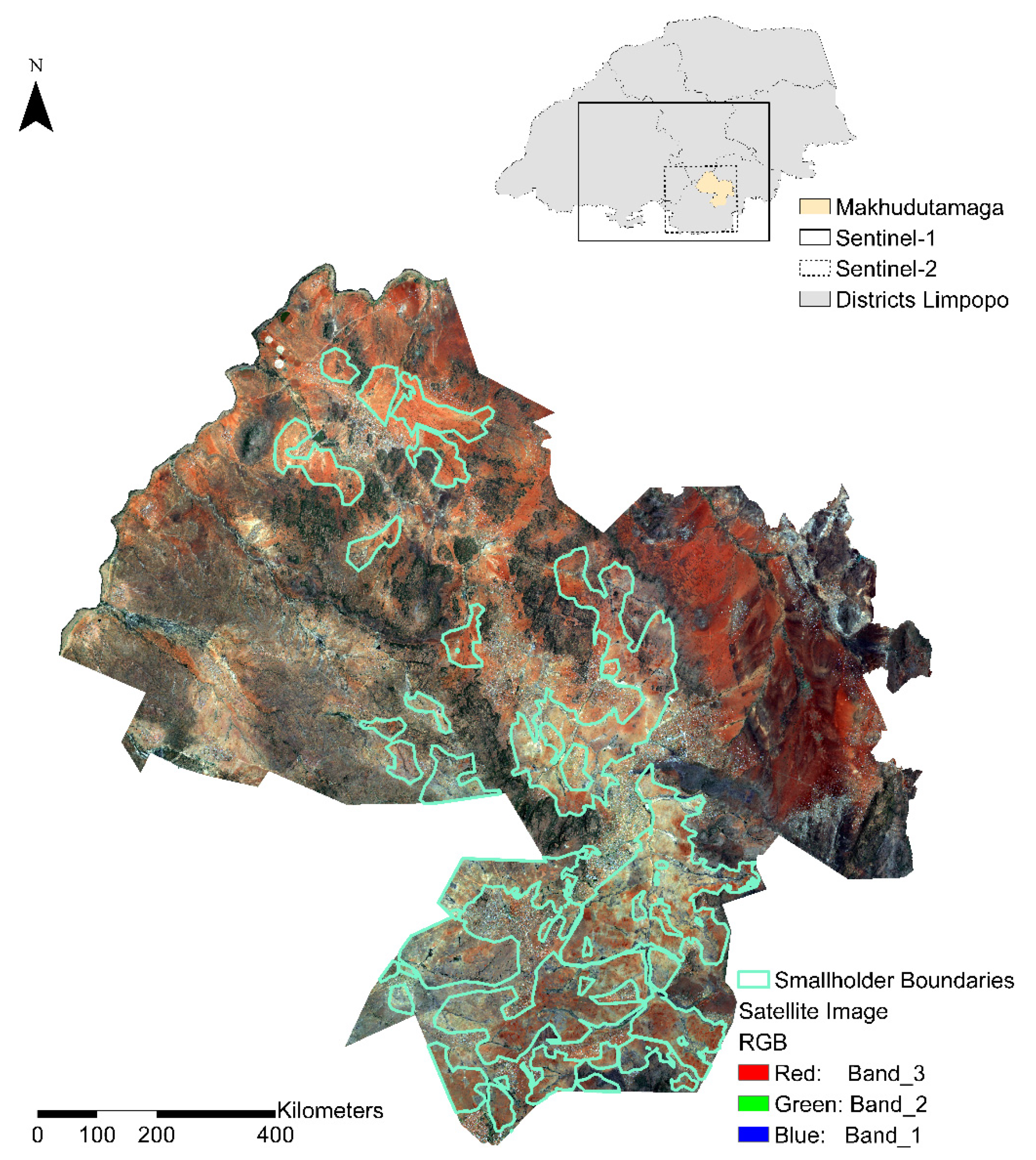
3.1. Study Area and Field Data Collection

Limpopo province is located on the northern part of South Africa. This province hosts Makhuduthamaga (Figure 1), which is the focus of this study. The area has rural villages that focus on smallholder maize farming [39]. Hence, due to the dominance of smallholder farms in the area, it was selected as a case study. Weather stations from the Agricultural Research Council located in Nchabeleng, Ga-Rantho, and Leeuwkraal have recorded an average annual rainfall of 536 mm and average annual temperatures of 7 °C in winter and 35 °C in summer. Makhuduthamaga has an undulating topography with rock habitats in the form of rock outcrops, rocky ridges, rocky flats, and rocky refugia [40].
Field surveys for the collection of training and validation data for different landcover types within the smallholder boundaries occurred from 18 to 21 February 2019. A handheld Garmin Global Positioning System (GPS) device which has a positional accuracy of 1.5 meters (on average mode) used to capture the coordinates of different land cover classes. The dominant land cover classes in the study area were captured; these include maize, bare land, and vegetation. The bare land and vegetation classes were combined to generate training samples (n = 9895 pixels) for the non-planted areas. The maize class consisted of n = 9802 pixels training samples. The samples were randomly selected into 80% training and 20% validation for each class. Constraining the land cover classes to two classes reduced the potential of classification errors from using the classes individually due to the variations in the natural occurrence of certain features. Limiting the area of investigation to the smallholder boundary excluded the farming activities in residents’ backyards, thus only land that was demarcated as smallholder farmland was considered. A total of 18 smallholder farms were randomly selected in the field for validation purposes. Their areas were measured using a GPS. Most of these farms do not have proper access roads, which made it difficult to survey more farms.

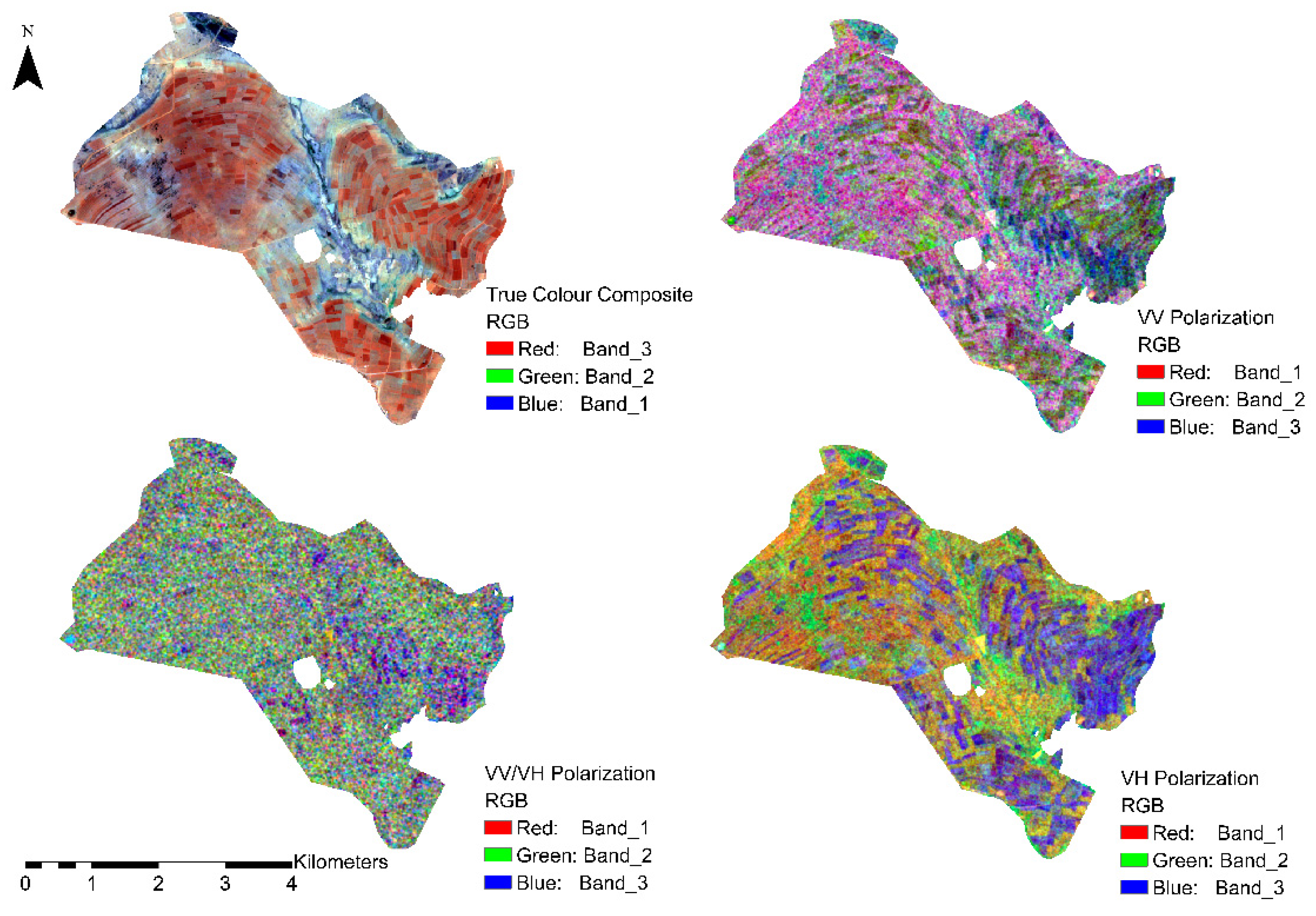
3.2. Sentinel-1 Data Acquisition and Pre-Processing

Sentinel-1 consists of a constellation of two satellites—Sentinel-1A and Sentinel-1B—which carry C-band SAR instruments to observe the Earth’s surface. Sentinel-1 has a frequent repeat cycle of 12 days and the repeat cycle of the two-satellite constellation can offer a 6 day repeat cycle depending on the availability of observations from both of them [41]. The advantages of this configuration in the current study is that Sentinel-1 can capture the spatio-temporal variations of smallholder farms. This study used Sentinel-1 Level-1 Ground Range Detected (GRD) images, which cover the maize cropping season (November 2018–July 2019) inclusive of all the smallholder farms. These images were 22 in total, and they were acquired from the Copernicus Open Access Hub in the Interferometric Wide (IW) mode. Both the VV and VH polarizations with a 10 m spatial resolution were used.
Pre-processing of the radar images was done in the Sentinel Application Platform (SNAP) according to Filipponi [42]. Firstly, the orbit files were applied to update the orbit state vectors in the metadata files. Secondly, radiometric calibration was done by applying annotated image calibration constants to convert the intensity values into sigma nought values. Thirdly, speckle filtering was performed to reduce the granular noise caused by many scatters. Fourthly, the geometric distortions caused by topography were corrected for using the Range Doppler terrain correction with a 3 sec Shuttle Radar Topography Mission (SRTM) Digital Elevation Model (DEM). Finally, the two polarizations (VV and VH) were converted from a linear scale to a decibel scale and the ratio VV/VH was calculated.
Figure 2 illustrates the mean polarizations for selected planted maize farms and non-planted maize areas during the planting season. The mean backscatter values for the VV, VH, and VV/VH polarizations for maize are −13.66, −20.14, and 0.68 dB, respectively. The aggregated class has mean values of −14.83, −20.67, and 0.72 dB for VV, VH, and VV/VH polarizations, respectively. The VH polarization has the highest variance of 6.31 dB compared to VV polarization with 2.65 dB and the VV/VH ratio with 0.0009 dB. The VH polarization seems to respond more effectively to the growing stages of maize. A similar observation was made by Son et al. [43] when they studied the rice crop also using Sentinel-1 data. This response is attributed to an increase in the volumetric structure of maize, which increases multiple reflections of the incoming signal.

3.3. Machine Learning Algorithms

The SVMs are advanced non-parametric statistical learning kernel-based algorithms commonly used in classification of remote sensing data [44,45]. Training data are projected into a higher-dimensional space using a linear/kernel-based function to optimally separate classes [43]. Parameters that optimally define the linear/non-linear hyperplane to separate the target classes are determined through an optimization problem. New data are evaluated based on the defined hyperplane constraints and categorized accordingly. The SVM requires regularization parameters that assist in tuning the model. These are C and gamma values, which were determined by the grid search method. In this study, the regularization parameter was 100, the gamma value was 0.01, and a Radial Basis Function (RBF) kernel was used. A comprehensive review of the tuning method can be found in Mountrakis et al. [46].
The Xgboost is part of the classification and regression ensemble gradient boosting machines (e.g., Gradient Boosting and AdaBoost). This boosting technique is an improved version of Gradient Boosting and AdaBoost because it has a higher computational efficiency and improved capacity to deal with over-fitting. For example, Xgboost grows trees parallel to each other, whereas the original Gradient Boosting model builds the trees in a series configuration [23,36,47]. Boosting uses many weak classifiers to produce a powerful classifier in an additive manner. The classifiers are trained on the weighted versions of the training sample; misclassified data are given more weight during the iteration process so that the next step focuses on the misclassified data [23]. The predictions improve over time and the final predictions are decided through a majority voting process to create vigorous predictions. This algorithm contains a rigorous number of regularization parameters that can be tuned to improve predictions and minimize overfitting [48]. These parameters are also determined using a grid search method.

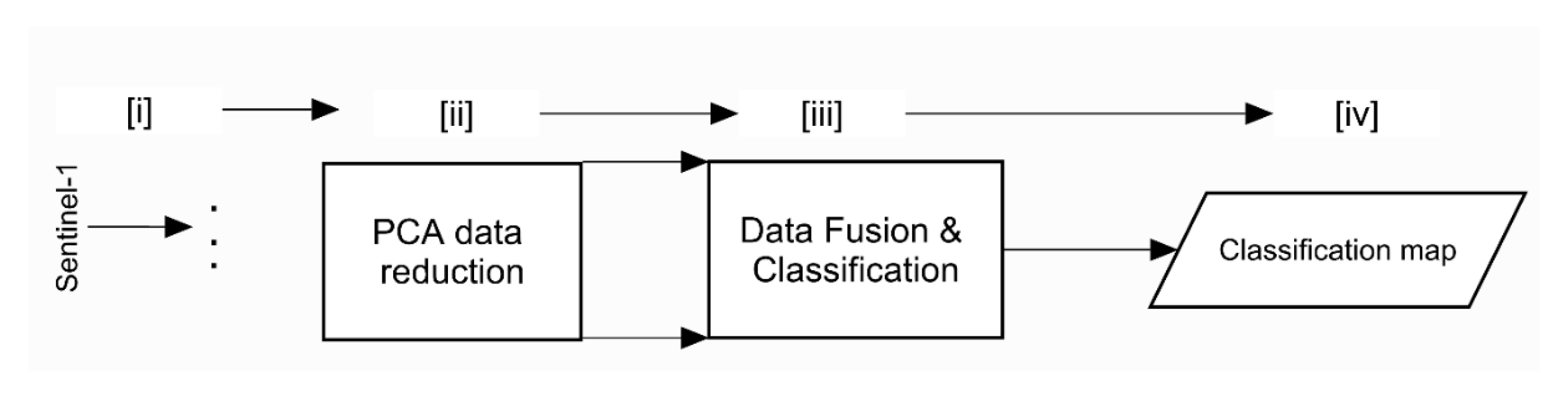
3.4. Experimental Design

The experimental design scheme is illustrated in Figure 3. The first stage (i) involves preparation and pre-processing of Sentinel-1 images as described in Section 3.2. The second stage (ii) pixel-based PCA image fusion, which reduces the dimensions of the multi-temporal Sentinel-1 images into only 3 bands (i.e., principal components 1, 2, and 3). The bands describe more than 70% of the information contained in the multi-temporal images (Figure 4). The selection criteria were motivated by reducing the computational demands on the system, without compromising on the accuracy of the results. The third stage (iii) entails model-level data fusion and application of SVM and Xgboost classification algorithms. The last stage (iv) is the generation of the classification map. The second stage (ii) is necessary to reduce computational demands and Random Access Memory (RAM) requirements. The third stage (iii) involves model-level data fusion using machine learning algorithms as described in Section 3.3. The data were separated into training (80%) and testing (20%) [49]. The performance and results of the algorithms in different experiments are compared using well-known evaluation metrics. This experiment was implemented using a Python programming platform on a Ryzen 9 3900, 12 cores processor at 3.8 GHz and 128 GB RAM computer.

3.5. Accuracy Assessment and Smallholder Maize Area Estimation

The models and experiments were evaluated using standard statistical analysis, i.e., confusion matrix, cross-validation, overall accuracy, precision, recall, F1-Score, and McNemar’s test [50,51]. These statistical measures have been used to evaluate different machine learning algorithms, such examples include, but are not limited to, Petropoulos et al. [52], Tong et al. [53], and Cucho-Padin et al. [54].
The confusion matrix is constructed by comparing the results from the classification algorithm with the reference data collected in the field [55]. The matrix can be used to derive accuracy statistics for the map. Such statistical values include overall accuracy, kappa coefficient of agreement ( k ^ ), and conditional kappa coefficient of agreement ( k ^ i ). These values are computed using Equations (1), (2), and (3 according to Congalton and Green [56]):
Overall   accuracy = i = 1 k x i i N ,
k ^ = N i = 1 k x i i i = 1 k ( x i + × x + j ) N 2 i = 1 k ( x i + × x + j ) ,
k ^ i = N ( x i i ) ( x i + × x + j ) N ( x i + ) ( x i + × x + j ) ,
where k is the land cover classes in the confusion matrix, x i + and x + j represent marginal total for row i and column j. x i i represents the number of observations in row i and column i. N represents total number of samples. The overall accuracy describes the proportion of the area mapped correctly. It provides a user with a probability that a randomly selected location on a map is correctly classified [57]. Kappa values that are more than 80% indicate good agreement between the reference and derived classification map. The k ^ measures the overall level of agreement between the reference data and the model data. The k ^ i allows computation of the level of agreement between the reference data and the model data for a specific class i.
Precision measures the ability of the algorithm not to label a true positive sample ( t p ) or a sample that is false positive ( f p ). Recall measures the ability of the algorithm to find all the true positives, and false negative is represented by f n . F1-Score is the harmonic mean calculated from both precision and recall values. These statistical values are calculated according to Equation (4) [55,58,59]:
precision   =   t p t p + f p , recall   =   t p t p + f n , F 1 - Score   =   ( 1 + β 2 ) p r e c i s i o n × r e c a l l β 2 × p r e c i s i o n + r e c a l l , where   β = 1 .
Cross-validation is another statistical method used to evaluate the performance of the model by dividing the data into k-folds (e.g., a standard value of 10 folds was used); the algorithm uses one set of data as training and the other sets are used to evaluate the model. During this iterative process, the accuracy score is calculated. The final cross-validation value is derived of the average accuracies from each iterative process. The superiority and significance between the SVM and Xgboost algorithms for each experiment were evaluated using a non-parametric McNemar’s statistical test [60,61,62]. The test is based on chi-square (χ2) statistics, calculated using Equation (5):
χ 2 = ( | f 12 f 21 | 1 ) 2 ( f 12 + f 21 ) ,
where f 12 denotes the number of cases that are wrongly classified by Model 1 but correctly classified by Model 2, and f 21 denotes the number of cases that are correctly classified by Model 1 but wrongly classified by Model 2 [63]. This was computed from two contingency matrices from the two algorithms that were being tested.
The unbiased proportional mapped areas were estimated using the method described by Olofsson et al. [57]. This method takes into account errors in misclassifications as reported in a confusion matrix. The mapped areas are estimated at 95% confidence intervals, and this is useful in providing error margins for the estimated areas for the end-users. Additional validation of the classification models’ ability to estimate smallholder maize was done. The areas measured at 18 smallholder farms were compared to the estimated areas from the SVM and Xgboost algorithms through a linear regression model. The p-value (p) and Pearson correlation coefficient (R) were derived to evaluate the agreement.

4. Results

4.1. Accuracy Assessment

A two-stage data fusion approach was used in this study, utilizing a time-series of Sentinel-1 polarization datasets. The SVM and Xgboost accuracy assessment results are listed in Table 2. The SVM has an overall accuracy of 97.1%, cross-validation score value of 89%, kappa value of 93.3%, and the conditional kappa coefficient of agreement of 90.54% and 95.7% for maize and non-planted classes, respectively. The Xgboost has an overall accuracy of 96.8%, cross-validation score value of 96%, kappa value of 92.6%, and conditional kappa coefficient of agreement of 90.4% and 94.4% for maize and non-planted classes, respectively. The maize classified pixels were similar for both classifiers based on the confusion matrix. The precision, recall, and F1-Score values for both algorithms have similar values that are more than 90% for both classes. It can also be noted that the recall for the planted maize class in both cases is approximately 3.7% lower compared to the precision score value. This observation is also supported by the kappa statistic and suggests that the planted maize class is less accurately classified compared to the non-planted class.
These results show that the SVM and Xgboost produced an acceptable performance in mapping smallholder farms and illustrated the capability of two-stage image fusion employed in this study. In particular, both algorithms classified the non-planted area class better by approximately 5% compared to the planted maize class. The cross-validation score indicates that the Xgboost algorithm is more consistent and stable compared to the SVM algorithm. The Xgboost algorithm cross-validation score outperformed the SVM algorithm cross-validation score by 7%. This is in contrast with the other statistical measures (Table 2), which seem to suggest that SVM has outperformed the Xgboost algorithm.
In situations where statistical evaluation matrices seem to contradict each other, a non-parametric statistical test must be conducted. In our case, we used McNemar’s significance test. If the estimated test statistic is lower than the critical chi-square table value (i.e., 3.84 at 95% confidence level), the null-hypothesis is rejected and it is concluded that there is no significant difference between the two model results [64]. The McNemar’s chi-square value of 64.62 and p-value of 9.085 × 10⁻¹⁶ were obtained by comparing the two algorithms. We, therefore, reject the null-hypothesis and conclude that the two results are statistically different from each other.

4.2. Variable Importance

Permutation variable importance was used to compute variable importance using the two estimators (SVM and Xgboost). The permutation algorithm can be defined to be the decrease in a model score when a single feature value is randomly shuffled [65]. Variable importance for each VV, VH, and VV/VH PCA 1, 2, and 3 polarizations are depicted in Figure 5. The VH and VV PCA polarizations formed the top six most important variables and the least important variables were the VV/VH PCA ratios. Specifically, the VH PCA 3 received the highest score, followed by the VV PCA 1 and VH PCA 2. The dominance of VH and VV polarizations was expected. Figure 6 depicts the VV, VH, and VV/VH PCA polarization composites. Smallholder maize farms are clearly enhanced by the VV and VH PCA polarization composites compared to the VV/VH polarizations.

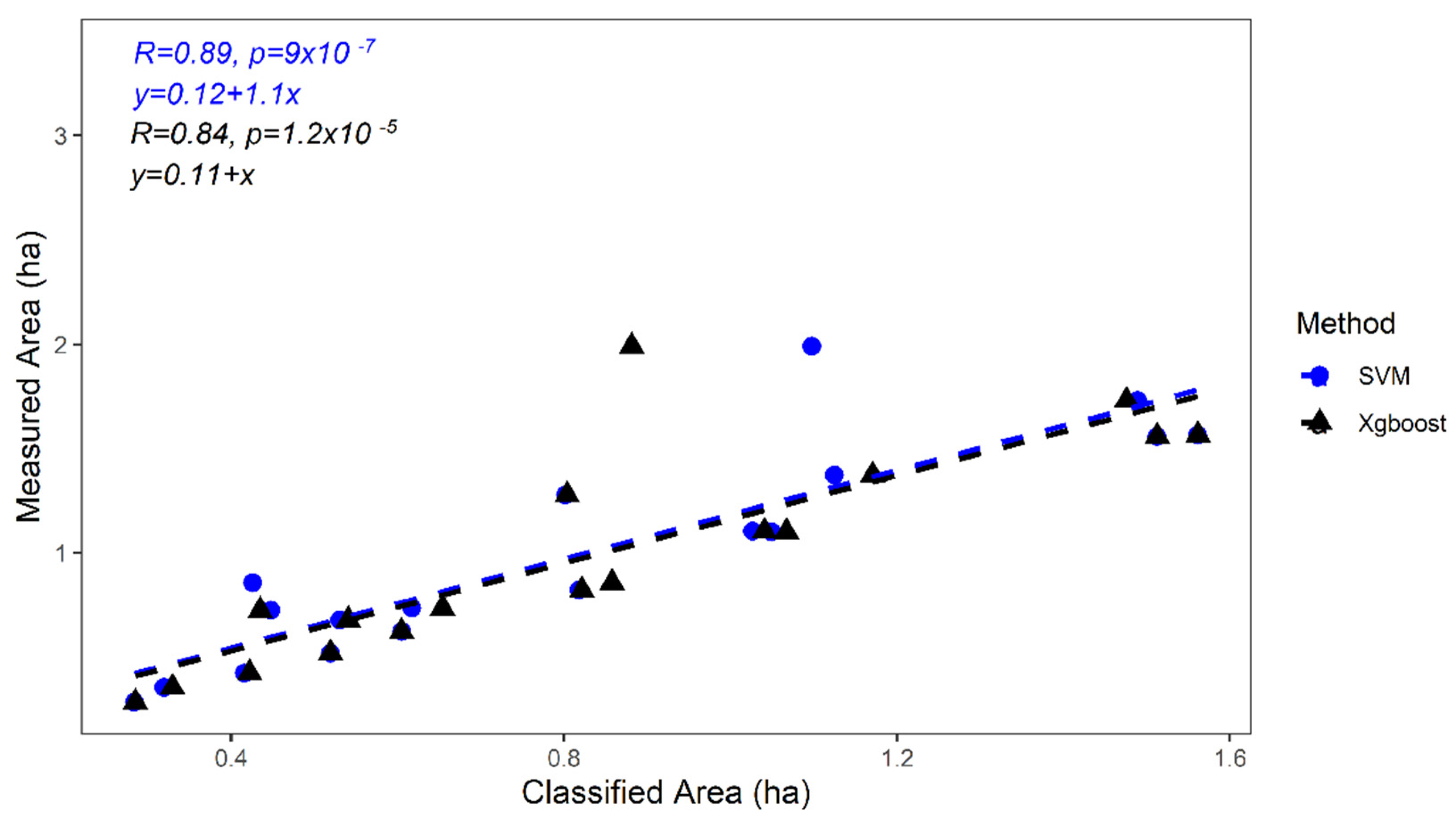
4.3. Mapping and Area Estimate for Smallholder Maize Farms

The maps for the maize planted areas produced by the SVM and Xgboost algorithms are depicted in Figure 7. The classification maps reveal the spatial distribution of the smallholder maize farms in our study area. It can be seen that most farmers that planted maize during the 2018/2019 season are from the south eastern part of Makhuduthamaga. These observations are consistent with both maps that were produced by the two algorithms. Visual inspection reveals no obvious disagreement between the two maps as predicted by the SVM and Xgboost algorithms.
The unbiased proportional areas were generated. The SVM algorithm estimated the planted maize class to be 7073.558 ± 0.01 ha and the non-planted class was estimated to be 33420.96 ± 0.01 ha. Meanwhile, the Xgboost estimated the planted maize class area to be 7303.32 ± 0.180 ha and the non-planted class was estimated to be 33191.2 ± 0.820 ha. It is worth noting that the SVM algorithm has better error margins (0.01 ha) for both classes compared to the Xgboost algorithm, which has error margins of 0.18 and 0.82 ha for the planted maize class and non-planted areas, respectively. The areas for the 18 smallholder farms (Figure 8) compared well with those generated by the classification models. The SVM classifier had a better fit (R = 0.89) in comparison with the Xgboost algorithm (R = 0.84). The linear model was an ideal fit for the data. The positive relationship was significant at a 95% level (p < 0.5).

5. Discussion

This study used Sentinel-1 multi-temporal datasets to map smallholder maize farm spatial distribution and to estimate maize production area for the maize crop. A two-staged image fusion technique was employed. The first stage involved using a pixel-based PCA technique to transform the original multi-temporal backscatter values into three component images that explained more than 70% of the information. This was done for the VV, VH, and VV/VH polarizations. The second stage involved model-level fusion, where all the components were used as input features into the machine learning algorithms. The SVM and Xgboost algorithms were used as classifiers to map the distribution of the maize farms and production area in Makhuduthamaga of Limpopo province, South Africa. This study found that Sentinel-1 had a high capacity to map smallholder maize planted areas with the application of machine learning algorithms. Furthermore, the two processing strategies used in this study detected smallholder maize farms with acceptable accuracy.
The accuracy assessment results were also expected. The overall accuracies were better than 90%, the cross-validation scores were greater than 85%, and the kappa coefficient of agreement and conditional kappa coefficient of agreement were all better than 90%. These results confirm the suitability of our approach in mapping smallholder farms using Sentinel-1 multi-temporal datasets. Other studies such as Ndikumana et al. [66] used Sentinel-1 multi-temporal data to map agricultural crops by applying a Deep Recurrent Neural Network and obtained favorable results that were better than 85% in accuracy. The SVM and Xgboost algorithms estimated maize production areas to be 7073.558 ± 0.01 ha and 7303.32 ± 0.180 ha, respectively. These values are relatively comparable to each other and SVM seems to have smaller error margins at a 95% confidence level and slightly higher overall accuracy than the Xgboost. However, for cross-validation scores, the Xgboost performed better. McNemar’s test showed that the results from the two algorithms were statistically different from each other. Other authors have evaluated different machine learning algorithms and obtained mixed performance indicators. Aguilar et al. [67] used different ensemble classifiers (Random Forest, SVM, and Majority Voting) to map smallholder farming systems based on the cloud-based multi-temporal approach and obtained overall accuracies ranging from 60% to 72%. Dong et al. [68] used Xgboost algorithms together with Decision Tree, Random Forest, and SVM to map land cover using Gaofen-3 Polarimetric SAR (PolSAR) data and obtained overall accuracies ranging from 88.4% to 93%. Zhong et al. [69] used machine learning algorithms and Deep Neural Network algorithms to map crop types and found that a Convolutional Neural Network model achieved 85.5%, while the Xgboost achieved 82.4% in overall accuracy under a multi-temporal classification scenario. Overall, the results produced by the classification algorithms compared favorably with the ground-based measured areas. Both algorithms had an agreement of more than 80%.
There are a few factors that may have contributed to the mapping errors as produced by the two algorithms and the radar data. Examples of these include, but are not limited to, loss of information during the PCA data reduction stage, backscatter mixing, and different planting patterns. Dimensional reduction may have contributed to the mapping errors. However, the three components that were kept for each polarization at more than 70% proved sufficient in our study. According to Woodhouse [16], backscatter intensity is sensitive to variations in scattering geometry, distribution of scatterer size, surface reflectivity beneath the canopy, leaf area density, row structure, and orientation relative to the range domain of the radar. Smallholder farms normally practice crop mixing, un-equal row planting patterns, and lack of irrigation systems. These practices can influence the backscatter intensity from maize. Scattering from nearby vegetation, such as grass and soil-canopy multiple scattering, can also contribute towards misclassification.
We showed that the PCA data reduction method can be used to facilitate the mapping of smallholder maize farms. Machine learning algorithms require data that can be separable to successfully classify data into their respective classes [50]. The PCA provides this by decorrelating the multi-temporal backscatter values into components that describe unique information for different classes, therefore enhancing the probability of accurate classification. Maize can grow up to an average height of 2 m and the structural volume of the crop also increases as the leaves also grow. This makes it possible to map maize with radar data, since the VV and VH polarizations are sensitive to vegetation structure and volumetric changes [70]. A frequent revisit of Sentinel-1 of 10–12 days and its high spatial resolution of 10 meters can capture the phenological stages of maize [41]. The increase in backscatter intensity for the maize class makes it possible to map smallholder farms in complex environments. PCA also suppresses other classes with low variable backscatter over time; these classes include grasslands and bare soil in our study area. The PCA image composites provide clear examples, where the advantage of the first stage of image fusion used in this study can be seen (Figure 6). The high level of importance of VH and VV polarizations were expected. Other studies, such as Arias et al. [71], illustrated that the VH, VV, and VH/VV polarizations ranked differently depending on the type of crop that was investigated. VH polarization was more suitable for rice and rapeseed discrimination, VV polarization was more suitable for alfalfa, and the VH/VV ratio was suitable for discriminating crops from different seasons.
The results can be used to generate spatial agricultural information such as estimating crop production areas and their spatial distributions in areas where survey datasets are not available, such as in our study. The results can be used to inform local government about the levels of agricultural activities in rural communities, thus providing ways to forecast food shortages and improve food security. The use of Sentinel-1 multi-temporal data provides an opportunity to afford this critical information regardless of the environmental conditions such as clouds or lack of extensive reference data. These results can also be used to contribute towards the SDG number 2. We therefore recommend the use of Sentinel-1 multi-temporal data to map smallholder farms at a provincial scale. More studies need to be done to explore the phase and amplitude data extracted from the backscatter intensities and their contribution to the accuracy of classifying smallholder farms. Different image fusion techniques and multi-sensor data fusion should also be explored.
The limitation of this study was that there were no agricultural statistics to independently validate the areas obtained by the machine learning algorithms. These validation data are normally collected by local agricultural departments. For example, the United States Department of Agriculture (USDA) uses remote sensing and extensive reference data provided by the National Agricultural Statistics Service (NASS) to generate the crop layer and associated statistics [72]. In areas with limited reference data, such as smallholder farms in developing countries, remote sensing technology provides a sustainable way to generate agricultural statistics with reasonable accuracies [18,20]. Processing multi-temporal data requires computational resources that are otherwise not easily accessible in developing countries. The Google Earth Engine (GEE) and other platforms provide an alternative solution to process data online, and these platforms allow for large-scale data processing at a relatively low cost. For example, Jin et al. [35] used the GEE platform to process Sentinel-1 data to map smallholder maize farms.
Future work should focus on testing this approach in different areas where smallholder farms are dominant. The response and efficiency of this approach should also be tested on different crop types. The operational model should be developed to consider the time domain when forecasting smallholder maize production areas. The phase and amplitude data from multi-temporal Sentinel-1 data and multi-sensor data should be explored in mapping smallholder farms in the future. These research opportunities will ensure that remote sensing technology can be fully utilized to support SDGs.

6. Conclusions

This study presented Sentinel-1 multi-temporal data for mapping smallholder maize farms’ spatial distribution and estimated production areas. The two-stage image fusion approach was adopted. The SVM and Xgboost machine learning algorithms were applied. The results revealed that most smallholder farms in our study area are distributed in the south eastern part of Makhuduthamaga. The algorithms provided comparable statistical evaluation results. However, McNemar’s test showed that the results from the two algorithms were statistically different from each other. The SVM and Xgboost algorithms estimated maize production areas to be 7073.558 ± 0.01 ha and 7303.32 ± 0.180 ha, respectively, for the region. The classified areas for selected farms compared favorably with the measured areas in the field and the SVM classifier had a better fit (R = 0.89) in comparison with the Xgboost algorithm (R = 0.84). The SVM algorithm seems to have generally performed better than the Xgboost algorithm. The use of multi-temporal Sentinel-1 with a two-stage image fusion approach proved to be effective in mapping smallholder farms. This framework can be used to support the SDGs and to provide spatial agricultural information to inform policy design and implementation by local government. Different seasons and different crop types should be tested using this approach, including extraction of phase and amplitude data from multi-temporal Sentinel-1 data. Multi-sensor data fusion should be explored to improve the mapping of smallholder farms in the future.

Author Contributions

Z.M.-M. conceptualized and developed the original draft of the manuscript. G.J.C. revised the manuscript, supervised, and provided financial resources for the project. C.M. was involved in data analysis and reviewed and edited the manuscript. All authors have read and agreed to the published version of the manuscript. The authors would like to thank the three anonymous reviewers for their valuable comments that improved the original manuscript.

Funding

This research was funded by the Agricultural Research Council, University of Pretoria and National Research Foundation (grant number: SFH170524232697 and TTK200221506319).

Data Availability Statement

Sentinel-1 data are freely available from the Copernicus Open Access Hub platform.

Conflicts of Interest

The authors declare no conflict of interest.

References

  1. Richard, C. The United Nations World Water Development Report 2015: Water for a Sustainable World; UNESCO Publishing: Paris, France, 2015; ISBN 9789231000713. [Google Scholar]
  2. Abraham, M.; Pingali, P. Transforming Smallholder Agriculture to Achieve the SDGs. In The Role of Smallholder Farms in Food and Nutrition Security; Gomez y Paloma, S., Riesgo, L., Louhichi, K., Eds.; Springer International Publishing: Berlin/Heidelberg, Germany, 2020; pp. 173–209. ISBN 9783030421489. [Google Scholar]
  3. Charman, A.; Hodge, J. Food Security in the SADC Region: An Assessment of National Trade Strategy in the Context of the 2001–03 Food Crisis. In Food Insecurity, Vulnerability and Human Rights Failure; Guha-Khasnobis, B., Acharya, S.S., Davis, B., Eds.; Studies in Development Economics and Policy; Palgrave Macmillan UK: London, UK, 2007; pp. 58–81. ISBN 9780230589506. [Google Scholar]
  4. FAO. (Ed.) Building Climate Resilience for Food Security and Nutrition. In The State of Food Security and Nutrition in the World; FAO: Rome, Italy, 2018; ISBN 9789251305713. [Google Scholar]
  5. FAO. Food and Agriculture Organization of the United Nations OECD-FAO Agricultural Outlook 2016–2025; FAO: Rome, Italy, 2016; ISBN 9789264259508. [Google Scholar]
  6. Jari, B.; Fraser, G.C.G. An Analysis of Institutional and Technical Factors Influencing Agricultural Marketing amongst Smallholder Farmers in the Kat River Valley, Eastern Cape Province, South Africa. Afr. J. Agric. Res. 2009, 4, 1129–1137. [Google Scholar] [CrossRef]
  7. Aliber, M.; Hall, R. Support for smallholder farmers in South Africa: Challenges of scale and strategy. Dev. S. Afr. 2012, 29, 548–562. [Google Scholar] [CrossRef]
  8. Calatayud, P.-A.; Le Ru, B.P.; Berg, J.V.D.; Schulthess, F. Ecology of the African Maize Stalk Borer, Busseola fusca (Lepidoptera: Noctuidae) with Special Reference to Insect-Plant Interactions. Insects 2014, 5, 539–563. [Google Scholar] [CrossRef] [Green Version]
  9. Giller, K.E.; Rowe, E.C.; de Ridder, N.; van Keulen, H. Resource use dynamics and interactions in the tropics: Scaling up in space and time. Agric. Syst. 2006, 88, 8–27. [Google Scholar] [CrossRef]
  10. Santpoort, R. The Drivers of Maize Area Expansion in Sub-Saharan Africa. How Policies to Boost Maize Production Overlook the Interests of Smallholder Farmers. Land 2020, 9, 68. [Google Scholar] [CrossRef] [Green Version]
  11. Kogan, F. Food Security: The Twenty-First Century Issue. In Promoting the Sustainable Development Goals in North American Cities; Metzler, J.B., Ed.; Springer: Berlin/Heidelberg, Germany, 2018; pp. 9–22. [Google Scholar]
  12. Liu, L.; Xiao, X.; Qin, Y.; Wang, J.; Xu, X.; Hu, Y.; Qiao, Z. Mapping cropping intensity in China using time series Landsat and Sentinel-2 images and Google Earth Engine. Remote Sens. Environ. 2020, 239, 111624. [Google Scholar] [CrossRef]
  13. Chakhar, A.; Ortega-Terol, D.; Hernández-López, D.; Ballesteros, R.; Ortega, J.F.; Moreno, M.A. Assessing the Accuracy of Multiple Classification Algorithms for Crop Classification Using Landsat-8 and Sentinel-2 Data. Remote Sens. 2020, 12, 1735. [Google Scholar] [CrossRef]
  14. Baret, F.; Weiss, M.; Lacaze, R.; Camacho, F.; Makhmara, H.; Pacholcyzk, P.; Smets, B. GEOV1: LAI and FAPAR essential climate variables and FCOVER global time series capitalizing over existing products. Part1: Principles of development and production. Remote Sens. Environ. 2013, 137, 299–309. [Google Scholar] [CrossRef]
  15. Campbell, J.B.; Wynne, R.H. Introduction to Remote Sensing, 5th ed.; Guilford Press: New York, NY, USA, 2011; ISBN 9781609181765. [Google Scholar]
  16. Woodhouse, I.H. Introduction to Microwave Remote Sensing; CRC Press: Boca Raton, FL, USA, 2017; ISBN 9781315272573. [Google Scholar]
  17. Attema, E.; Davidson, M.; Floury, N.; Levrini, G.; Rosich-Tell, B.; Rommen, B.; Snoeij, P. Sentinel-1 ESA’s new European SAR mission. Remote Sens. 2007, 6744, 674403. [Google Scholar] [CrossRef]
  18. Jain, M.; Mondal, P.; DeFries, R.S.; Small, C.G.; Galford, G.L. Mapping cropping intensity of smallholder farms: A comparison of methods using multiple sensors. Remote Sens. Environ. 2013, 134, 210–223. [Google Scholar] [CrossRef] [Green Version]
  19. McNairn, H.; Brisco, B. The application of C-band polarimetric SAR for agriculture: A review. Can. J. Remote Sens. 2004, 30, 525–542. [Google Scholar] [CrossRef]
  20. Useya, J.; Chen, S. Exploring the Potential of Mapping Cropping Patterns on Smallholder Scale Croplands Using Sentinel-1 SAR Data. Chin. Geogr. Sci. 2019, 29, 626–639. [Google Scholar] [CrossRef] [Green Version]
  21. Kenduiywo, B.K.; Bargiel, D.; Soergel, U. Crop-type mapping from a sequence of Sentinel 1 images. Int. J. Remote Sens. 2018, 39, 6383–6404. [Google Scholar] [CrossRef]
  22. Whelen, T.; Siqueira, P. Time-series classification of Sentinel-1 agricultural data over North Dakota. Remote Sens. Lett. 2018, 9, 411–420. [Google Scholar] [CrossRef]
  23. Chen, T.; Guestrin, C. XGBoost: A Scalable Tree Boosting System. In Proceedings of the 22nd ACM SIGKDD International Conference on Knowledge Discovery and Data Mining, San Francisco, CA, USA, 13 August 2016; pp. 785–794. [Google Scholar]
  24. Elith, J.; Leathwick, J.R.; Hastie, T. A working guide to boosted regression trees. J. Anim. Ecol. 2008, 77, 802–813. [Google Scholar] [CrossRef] [PubMed]
  25. Piiroinen, R.; Heiskanen, J.; Mõttus, M.; Pellikka, P. Classification of Crops across Heterogeneous Agricultural Landscape in Kenya Using AisaEAGLE Imaging Spectroscopy Data. Int. J. Appl. Earth Obs. Geoinf. 2015, 39, 1–8. [Google Scholar] [CrossRef]
  26. Licciardi, G.; Marpu, P.R.; Chanussot, J.; Benediktsson, J.A. Linear Versus Nonlinear PCA for the Classification of Hyperspectral Data Based on the Extended Morphological Profiles. IEEE Geosci. Remote. Sens. Lett. 2011, 9, 447–451. [Google Scholar] [CrossRef] [Green Version]
  27. Chatziantoniou, A.; Psomiadis, E.; Petropoulos, G.P. Co-Orbital Sentinel 1 and 2 for LULC Mapping with Emphasis on Wetlands in a Mediterranean Setting Based on Machine Learning. Remote Sens. 2017, 9, 1259. [Google Scholar] [CrossRef] [Green Version]
  28. Karthikeyan, L.; Chawla, I.; Mishra, A.K. A review of remote sensing applications in agriculture for food security: Crop growth and yield, irrigation, and crop losses. J. Hydrol. 2020, 586, 124905. [Google Scholar] [CrossRef]
  29. Mufungizi, A.A.; Musakwa, W.; Gumbo, T. A land suitability analysis of the vhembe district, south africa, the case of maize and sorghum. ISPRS Int. Arch. Photogramm. Remote. Sens. Spat. Inf. Sci. 2020, 43, 1023–1030. [Google Scholar] [CrossRef]
  30. Skakun, S.; Kalecinski, N.; Brown, M.; Johnson, D.; Vermote, E.; Roger, J.-C.; Franch, B. Assessing within-Field Corn and Soybean Yield Variability from WorldView-3, Planet, Sentinel-2, and Landsat 8 Satellite Imagery. Remote Sens. 2021, 13, 872. [Google Scholar] [CrossRef]
  31. Ji, Z.; Pan, Y.; Zhu, X.; Wang, J.; Li, Q. Prediction of Crop Yield Using Phenological Information Extracted from Remote Sensing Vegetation Index. Sensors 2021, 21, 1406. [Google Scholar] [CrossRef] [PubMed]
  32. Kavvada, A.; Metternicht, G.; Kerblat, F.; Mudau, N.; Haldorson, M.; Laldaparsad, S.; Friedl, L.; Held, A.; Chuvieco, E. Towards delivering on the Sustainable Development Goals using Earth observations. Remote Sens. Environ. 2020, 247, 111930. [Google Scholar] [CrossRef]
  33. Cochran, F.; Daniel, J.; Jackson, L.; Neale, A. Earth Observation-Based Ecosystem Services Indicators for National and Subnational Reporting of the Sustainable Development Goals. Remote Sens. Environ. 2020, 244, 111796. [Google Scholar] [CrossRef] [PubMed]
  34. Abubakar, G.A.; Wang, K.; Shahtahamssebi, A.; Xue, X.; Belete, M.; Gudo, A.J.A.; Shuka, K.A.M.; Gan, M. Mapping Maize Fields by Using Multi-Temporal Sentinel-1A and Sentinel-2A Images in Makarfi, Northern Nigeria, Africa. Sustainability 2020, 12, 2539. [Google Scholar] [CrossRef] [Green Version]
  35. Jin, Z.; Azzari, G.; You, C.; Di Tommaso, S.; Aston, S.; Burke, M.; Lobell, D.B. Smallholder maize area and yield mapping at national scales with Google Earth Engine. Remote Sens. Environ. 2019, 228, 115–128. [Google Scholar] [CrossRef]
  36. Polly, J.; Hegarty-Craver, M.; Rineer, J.; O’Neil, M.; Lapidus, D.; Beach, R.; Temple, D.S. The use of Sentinel-1 and -2 data for monitoring maize production in Rwanda. In Proceedings of the Remote Sensing for Agriculture, Ecosystems, and Hydrology XXI, Strasbourg, France, 21 October 2019; Volume 11149, p. 111491Y. [Google Scholar] [CrossRef]
  37. Abdi, H.; Williams, L.J. Principal component analysis. Wiley Interdiscip. Rev. Comput. Stat. 2010, 2, 433–459. [Google Scholar] [CrossRef]
  38. Canty, M.J. Image Analysis, Classification and Change Detection in Remote Sensing: With Algorithms for ENVI/IDL and Python, 3rd ed.; CRC Press: Boca Raton, FL, USA, 2014; ISBN 9781466570382. [Google Scholar]
  39. SDM. Greater Sekhukhune Cross Border District Municipality Integrated Development Plan: 2019/20; SDM: Sekhukhune, Limpopo, South Africa, 2019. [Google Scholar]
  40. Siebert, S.J.; Van Wyk, A.E.; Bredenkamp, G.J.; Siebert, F. Vegetation of the rock habitats of the Sekhukhuneland Centre of Plan Endemism, South Africa. Bothalia Pretoria 2003, 33, 207–228. [Google Scholar] [CrossRef] [Green Version]
  41. Torres, R.; Snoeij, P.; Geudtner, D.; Bibby, D.; Davidson, M.; Attema, E.; Potin, P.; Rommen, B.; Floury, N.; Brown, M.; et al. GMES Sentinel-1 mission. Remote Sens. Environ. 2012, 120, 9–24. [Google Scholar] [CrossRef]
  42. Filipponi, F. Sentinel-1 GRD Preprocessing Workflow. In Proceedings of the 3rd International Electronic Conference on Remote Sensing, Roma, Italy, 22 May–5 June 2019; Volume 18, p. 11. [Google Scholar] [CrossRef] [Green Version]
  43. Son, N.-T.; Chen, C.-F.; Chen, C.-R.; Minh, V.-Q. Assessment of Sentinel-1A data for rice crop classification using random forests and support vector machines. Geocarto Int. 2017, 1–32. [Google Scholar] [CrossRef]
  44. Foody, G.M.; Mathur, A. Toward intelligent training of supervised image classifications: Directing training data acquisition for SVM classification. Remote Sens. Environ. 2004, 93, 107–117. [Google Scholar] [CrossRef]
  45. Wan, S.; Chang, S.-H. Crop classification with WorldView-2 imagery using Support Vector Machine comparing texture analysis approaches and grey relational analysis in Jianan Plain, Taiwan. Int. J. Remote Sens. 2019, 40, 8076–8092. [Google Scholar] [CrossRef]
  46. Mountrakis, G.; Im, J.; Ogole, C. Support vector machines in remote sensing: A review. ISPRS J. Photogramm. Remote Sens. 2011, 66, 247–259. [Google Scholar] [CrossRef]
  47. Nobre, J.; Neves, R.F. Combining Principal Component Analysis, Discrete Wavelet Transform and XGBoost to Trade in the Financial Markets. Expert Syst. Appl. 2019, 125, 181–194. [Google Scholar] [CrossRef]
  48. Georganos, S.; Grippa, T.; VanHuysse, S.; Lennert, M.; Shimoni, M.; Wolff, E. Very High Resolution Object-Based Land Use–Land Cover Urban Classification Using Extreme Gradient Boosting. IEEE Geosci. Remote Sens. Lett. 2018, 15, 607–611. [Google Scholar] [CrossRef] [Green Version]
  49. Zhao, H.; Chen, Z.; Jiang, H.; Jing, W.; Sun, L.; Feng, M. Evaluation of Three Deep Learning Models for Early Crop Classification Using Sentinel-1A Imagery Time Series—A Case Study in Zhanjiang, China. Remote Sens. 2019, 11, 2673. [Google Scholar] [CrossRef] [Green Version]
  50. Skiena, S.S. Machine Learning. In The Data Science Design Manual; Skiena, S.S., Ed.; Texts in Computer Science; Springer International Publishing: Cham, Germany, 2017; pp. 351–390. ISBN 9783319554440. [Google Scholar]
  51. Aggarwal, C.C. (Ed.) Data Classification: Algorithms and Applications. In Data Mining and Knowledge Discovery Series; CRC Press: Boca Raton, FL, USA; Taylor & Francis Group: Boca Raton, FL, USA, 2014; ISBN 9781466586741. [Google Scholar]
  52. Petropoulos, G.P.; Kalaitzidis, C.; Vadrevu, K.P. Support vector machines and object-based classification for obtaining land-use/cover cartography from Hyperion hyperspectral imagery. Comput. Geosci. 2012, 41, 99–107. [Google Scholar] [CrossRef]
  53. Tong, X.-Y.; Xia, G.-S.; Lu, Q.; Shen, H.; Li, S.; You, S.; Zhang, L. Land-cover classification with high-resolution remote sensing images using transferable deep models. Remote Sens. Environ. 2020, 237, 111322. [Google Scholar] [CrossRef] [Green Version]
  54. Cucho-Padin, G.; Loayza, H.; Palacios, S.; Balcazar, M.; Carbajal, M.; Quiroz, R. Development of low-cost remote sensing tools and methods for supporting smallholder agriculture. Appl. Geomat. 2019, 12, 247–263. [Google Scholar] [CrossRef] [Green Version]
  55. Lewis, H.G.; Brown, M. A generalized confusion matrix for assessing area estimates from remotely sensed data. Int. J. Remote Sens. 2001, 22, 3223–3235. [Google Scholar] [CrossRef]
  56. Congalton, R.G.; Green, K. Assessing the Accuracy of Remotely Sensed Data Principles and Practices, 2nd ed; CRS Press: Boca Raton, FL, USA; Taylor and Francis Group: London, UK, 2008. [Google Scholar]
  57. Olofsson, P.; Foody, G.M.; Stehman, S.V.; Woodcock, C.E. Making better use of accuracy data in land change studies: Estimating accuracy and area and quantifying uncertainty using stratified estimation. Remote Sens. Environ. 2013, 129, 122–131. [Google Scholar] [CrossRef]
  58. Davis, J.; Goadrich, M. The relationship between Precision-Recall and ROC curves. In Proceedings of the 23rd International Conference on Machine Learning, Pittsburgh, PA, USA, 25–29 June 2006; pp. 233–240. [Google Scholar]
  59. Flach, P.; Kull, M. Precision-Recall-Gain Curves: PR Analysis Done Right. Advances in Neural Information Processing Systems; NIPS: Bristol, UK, 2015. [Google Scholar]
  60. McNemar, Q. Note on the sampling error of the difference between correlated proportions or percentages. Psychometrika 1947, 12, 153–157. [Google Scholar] [CrossRef] [PubMed]
  61. Edwards, A.L. Note on the “correction for continuity” in testing the significance of the difference between correlated proportions. Psychometrika 1948, 13, 185–187. [Google Scholar] [CrossRef] [PubMed]
  62. De Leeuw, J.; Jia, H.; Yang, L.; Liu, X.; Schmidt, K.; Skidmore, A.K. Comparing accuracy assessments to infer superiority of image classification methods. Int. J. Remote Sens. 2006, 27, 223–232. [Google Scholar] [CrossRef]
  63. Manandhar, R.; Odeh, I.O.A.; Ancev, T. Improving the Accuracy of Land Use and Land Cover Classification of Landsat Data Using Post-Classification Enhancement. Remote Sens. 2009, 1, 330–344. [Google Scholar] [CrossRef] [Green Version]
  64. Sahin, E.K.; Colkesen, I. Performance analysis of advanced decision tree-based ensemble learning algorithms for landslide susceptibility mapping. Geocarto Int. 2019, 1–23. [Google Scholar] [CrossRef]
  65. Breiman, L. Random Forests. Mach. Learn. 2001, 45, 5–32. [Google Scholar] [CrossRef] [Green Version]
  66. Ndikumana, E.; Minh, D.H.T.; Baghdadi, N.; Courault, D.; Hossard, L. Deep Recurrent Neural Network for Agricultural Classification using multitemporal SAR Sentinel-1 for Camargue, France. Remote Sens. 2018, 10, 1217. [Google Scholar] [CrossRef] [Green Version]
  67. Aguilar, R.; Zurita-Milla, R.; Izquierdo-Verdiguier, E.; De By, R.A. A Cloud-Based Multi-Temporal Ensemble Classifier to Map Smallholder Farming Systems. Remote Sens. 2018, 10, 729. [Google Scholar] [CrossRef] [Green Version]
  68. Dong, H.; Xu, X.; Wang, L.; Pu, F. Gaofen-3 PolSAR Image Classification via XGBoost and Polarimetric Spatial Information. Sensors 2018, 18, 611. [Google Scholar] [CrossRef] [Green Version]
  69. Zhong, L.; Hu, L.; Zhou, H. Deep learning based multi-temporal crop classification. Remote Sens. Environ. 2019, 221, 430–443. [Google Scholar] [CrossRef]
  70. McNairn, H.; Champagne, C.; Shang, J.; Holmstrom, D.; Reichert, G. Integration of optical and Synthetic Aperture Radar (SAR) imagery for delivering operational annual crop inventories. ISPRS J. Photogramm. Remote Sens. 2009, 64, 434–449. [Google Scholar] [CrossRef]
  71. Arias, M.; Campo-Bescós, M. Ángel; Álvarez-Mozos, J. Crop Classification Based on Temporal Signatures of Sentinel-1 Observations over Navarre Province, Spain. Remote Sens. 2020, 12, 278. [Google Scholar] [CrossRef] [Green Version]
  72. Boryan, C.; Yang, Z.; Mueller, R.; Craig, M. Monitoring US agriculture: The US Department of Agriculture, National Agricultural Statistics Service, Cropland Data Layer Program. Geocarto Int. 2011, 26, 341–358. [Google Scholar] [CrossRef]
Figure 1. Study area location map for Makhuduthamaga in Limpopo, South Africa.
Remotesensing 13 01666 g001
Figure 2. The mean raw VV, VH, and VV/VH backscatter profiles. The extracted polarizations are for maize crops and other classes, which refers to aggregated bare soil and grasslands.
Remotesensing 13 01666 g002
Figure 3. Schematic illustration of the experimental design.
Remotesensing 13 01666 g003
Figure 4. The variance explained by the VV, VH, and VV/VH components. The first three components, which explained greater than 70% of the variance, were selected.
Remotesensing 13 01666 g004
Figure 5. Permutation importance scores for the Principal Component Analysis (PCA)-derived images used in the analysis. PCA 3 for the VH polarization is the most important variable in our study. The same results were obtained for the two estimators.
Remotesensing 13 01666 g005
Figure 6. Examples of the PCA images for different polarizations derived from Sentinel-1 datasets. The PCA VH polarization composite seems to visually enhance smallholder farms compared to other polarizations.
Remotesensing 13 01666 g006
Figure 7. Planted maize crop maps produced by the SVM (a) and Xgboost (b) algorithms. Insert maps for SVM and Xgboost are represented by (c) and (d), respectively.
Remotesensing 13 01666 g007
Figure 8. Comparison of the field measured areas (y) to those generated by the classification models (x) applying the SVM and Xgboost algorithms.
Remotesensing 13 01666 g008
Table 1. A bibliometric search result of common result phrases and the associated number of documents retrieved. Time limit was not used in the search criteria.
Search Criteria (Limited to Article, Book Chapter, and Book) Scopus Web of Science Core Collection
TITLE-ABS-KEY (remote AND sensing AND maize OR corn) 16721942
TITLE-ABS-KEY (remote AND sensing AND sdgs) 4966
TITLE-ABS-KEY (remote AND sensing AND sdgs AND maize OR corn)11
TITLE-ABS-KEY (remote AND sensing AND maize OR corn AND smallholder) 3543
Table 2. Accuracy assessment produced for the Sentinel-1 multi-temporal classification using the Support Vector Machine (SVM) and Extreme Gradient Boosting (Xgboost) algorithms.
ModelOverall AccuracyCross-
Validation
Confusion Matrix
SVM Planted MaizeNon-Planted
0.9710.89 +/−0,0520,1391457
62850,790
Xgboost Planted MaizeNon-Planted
0.9680.96 +/−0.0220,1151481
82550,593
SVMXgboost
ClassesPlanted Maize Non-Planted Planted Maize Non-Planted
Precision0.970.9720.9610.972
Recall0.9330.9880.9310.984
F1-Score0.9510.980.9460.978
Publisher’s Note: MDPI stays neutral with regard to jurisdictional claims in published maps and institutional affiliations.

