
Joint Geoeffectiveness and Arrival Time Prediction of CMEs by a Unified Deep Learning Framework


1
Beijing Key Laboratory of Intelligent Telecommunications Software and Multimedia, Beijing University of Posts and Telecommunications, Beijing 100876, China
2
State Key Laboratory of Lunar and Planetary Sciences, Macau University of Science and Technology, Macao 999078, China
3
State Key Laboratory of Space Weather, National Space Science Center, Chinese Academy of Sciences, Beijing 100190, China
*
Author to whom correspondence should be addressed.
Remote Sens. 2021, 13(9), 1738; https://0-doi-org.brum.beds.ac.uk/10.3390/rs13091738
Submission received: 19 March 2021
/
Revised: 22 April 2021
/
Accepted: 27 April 2021
/
Published: 30 April 2021
(This article belongs to the Special Issue Space Weather: Observations and Modeling of the Near Earth Environment)
Abstract
:Fast and accurate prediction of the geoeffectiveness of coronal mass ejections (CMEs) and the arrival time of the geoeffective CMEs is urgent, to reduce the harm caused by CMEs. In this paper, we present a new deep learning framework based on time series of satellites’ optical observations that can give both the geoeffectiveness and the arrival time prediction of the CME events. It is the first time combining these two demands in a unified deep learning framework with no requirement of manually feature selection and get results immediately. The only input of the deep learning framework is the time series images from synchronized solar white-light and EUV observations. Our framework first uses the deep residual network embedded with the attention mechanism to extract feature maps for each observation image, then fuses the feature map of each image by the feature map fusion module and determines the geoeffectiveness of CME events. For the geoeffective CME events, we further predict its arrival time by the deep residual regression network based on group convolution. In order to train and evaluate our proposed framework, we collect 2400 partial-/full-halo CME events and its corresponding images from 1996 to 2018. The F1 score and Accuracy of the geoeffectiveness prediction can reach 0.270% and 75.1%, respectively, and the mean absolute error of the arrival time prediction is only 5.8 h, which are both significantly better than well-known deep learning methods and can be comparable to, or even better than, the best performance of traditional methods.
1. Introduction
Coronal Mass Ejections (CMEs) are fierce eruption phenomena in the solar atmosphere, which is one important source of severe space weather events [1]. When arriving at Earth, the magnetic field and plasma in a CME will disturb Earth’s space environment and may cause geomagnetic storms [2]. Magnetic storms are threats to the high-tech modern society, which relies on stable satellite communication, global navigation and electricity power supplements in almost every aspect [3]. To reduce the potential damages of CMEs, a reliable forecasting model is necessary. Generally speaking, it takes 1–5 days for CMEs to propagate from the Sun to Earth, which makes it theoretically feasible to predict its geoeffectiveness and the arrival time in advance.
Many efforts have been made to achieve a fast and accurate forecast in traditional methods. Based on the observations from Large Angle and Spectrometric Coronagraph (LASCO) onboard the Solar and Heliospheric Observatory (SOHO) [4], many empirical models have been developed, such as the empirical shock arrival (ESA) [5] model, the Cone model [6] and Self-similar Expansion model [7]. These models are based on the math-fit of observed morphology evolution of CMEs in the coronagraph and with a presumed propagation model. Although limited by the projection effects [8] from one single coronagraph, these models’ correctness and arrival time prediction is acceptable. The launch of the Solar-Terrestrial Relations Observatory (STEREO) [9] twin star provides additional view points away from the Sun–Earth line. With the observations from the Heliosphere Imagers (HIs) [10], the projection effects have been further reduced and the improved empirical models have been proven to be adequately effective [11]. Most of the empirical models are mathematical models with no requirement of background heliospheric measurements. Hydrodynamic models, like the drag-based model [12] and shock-based models [13,14], take into consideration the acceleration or deceleration of a CME caused by the ambient solar wind. However, those models are kinetic models without magnetic fields and with limited physical meanings, and the solar wind parameters used as input in these models need to be measured in-situ or manually set based on historical measurements. This situation was changed by magnetohydrodynamics (MHD) [15,16,17] models. With properly set input parameters and boundary conditions, a MHD model could track the whole transit of a CME from the Sun to the Earth at the cost of high computing power consumption [18]. The demands of supercomputers make such forecast models hard to distribute and to give a near real-time forecast.
In recent years, with the continuous development of machine learning and deep learning, related methods have also been applied to geoeffectiveness and arrival time prediction of CMEs. Besliu-Ionescu et al. [19] attempts to use the logistic regression which uses only initial CME parameters as input to predict the geoeffectiveness of CMEs, but it doesn’t fit well on the training set. Sudar et al. [20] uses the fully connected neural network (FCNN) to analyse the transit time for 153 CME events using the initial velocity of the CME and the central meridian distance of the associated flare as inputs, the mean absolute error (MAE) obtained is about 11.6 h. Liu et al. [21] uses the support vector machine (SVM) [22] to predict the arrival time for 182 geoeffective partial-/full-halo CME events, and the MAE is about 5.9 h. However, 5.9 h is the best result in a random 100,000 testing set. The above machine learning methods require manual collection of parameters and if the relevant parameters are missing, it may cause a wide range of errors. Wang et al. [23] first uses the convolutional neural network to estimate the arrival time of geoeffective CME events based on satellite observation images. It only uses the SOHO LASCO C2 white-light corona observations as input, and the error was about 12.4 h. Although the error is large, the input is a directly observed image, which simplifies the tedious work of manual feature acquisition. All above-mentioned four methods have certain limitations, mainly in that they can only predict the geoeffectiveness of CMEs or can only predict the transit/arrival-time of CME events that can reach Earth, and do not combine the two demands in a machine learning or deep learning method.
With the introduction of large image data sets such as ImageNet [24] and MS-COCO [25], many simple, highly modularized convolutional neural networks architecture [26,27,28,29,30,31,32,33,34,35] have been proposed in the field of computer vision. VGGNet [27] uses a stack of very small () convolution filters to increase the depth of the network, and explore the impact of depth on network performance. Resnet [28] presents a residual learning framework to make the deep neural network easier to train, and make the gradient back propagated by the model have better local correlation [36]. GoogLeNet [29] proposes the Inception module, which increases the width and depth of the network without increasing the computational budget and improves the adaptability of the network to different scales through multi-scale processing. Resnext [31] combines the idea of the Inception module with the residual learning, and improves the performance of the model by increasing the cardinality. Mobilenet [32] builds a lightweight deep neural network through depth-wise separable convolutions.
In this paper, we present a deep learning framework based on time series of satellites’ optical observations that can give both the geoeffectiveness and the arrival time prediction of the CME events. The framework is composed of the collection of time series observation images, the geoeffectiveness prediction algorithm and arrival time prediction algorithm. The contributions of this paper are summarized as follows:
- (1)
- It is the first time that making geoeffectiveness and arrival time predictions of CMEs in a unified deep learning framework and forming an end-to-end prediction. Once we get the observation images, we can immediately get the prediction result without selecting features manually or professional knowledge.
- (2)
- For the geoeffectiveness prediction of CMEs, we propose a deep residual network embedded with the attention mechanism and the feature map fusion module. Based on those, we can effectively extract key regional features and fuse the feature from each image.
- (3)
- For the arrival time prediction of geoeffective CMEs, we propose a data expansion method to increase the scale of data and deep residual regression network to capture the feature of the observation image. Meanwhile, the cost-sensitive regression loss function is proposed to allow the network focus more attention on hard predicting samples.
The remainder of this paper is organized as follows—in Section 2, we introduce our proposed deep learning framework in detail. Section 3 describes the dataset and experimental setting. The experimental results and comparisons are reported in Section 4. Section 5 and Section 6 are the discussion and conclusion, respectively.
2. Methods
The overall deep learning framework is shown in Figure 1. When predicting the geoeffectiveness and arrival time of the CME events, we first collect the corresponding satellite observation images from 10 min before up to 4 h after the onset time of the CME events and feed them into the deep learning framework as the only input.
Then our framework determines the geoeffectiveness of the CME event. Specifically, we use the deep residual network embedded with the attention mechanism which plays the role of feature extraction module in geoeffectiveness prediction to extract the feature map for each observation image. Since the number of observation images collected in each CME event is not fixed (see the details in Section 3.1), we use the feature map fusion module to fuse the feature maps of each input image into a fused feature map, and predict the probability that the CME event is geoeffective or not. If the probability is greater than 0.5, it is judged as a geoeffective CME event.
For a geoeffective CME event, our framework further predicts its arrival time by predicting the arrival time of each image in the CME event and taking the average. Specifically, we first use the deep residual regression network based on group convolution to extract the feature map of each image, and then predict the transit time of each image. The predicted arrival time of each image can be obtained through the predicted transit time plus the observation time of the image, and the average predicted arrival time of all input images in the CME event is taken as the predicted arrival time of the CME event. The reason for adopting this strategy is to prevent the problem of under-fitting of the CME arrival time prediction network due to fewer geoeffective samples and the detailed reasons can be seen in Section 2.2.1.
2.1. Geoeffectiveness Prediction of CMEs
2.1.1. Deep Residual Network Embedded with the Attention Mechanism
The proposed deep residual network embedded with the attention mechanism is used to extract the feature map from each observation image. Our network is designed based on the traditional convolutional neural networks and modified to make it more suitable for CME observation images. The main features are as follows—compared with ImageNet, the features of the CME image are more sparse, so we select larger convolution filters; using the residual learning to train a deeper network; introducing the attention mechanism to extract key area features.
The input image will first pass through data preprocessing. It consists of scaling, normalization and gray scale conversion. After that, the input image will be a gray scale image and pixel size is , and the weight of each pixel is between [0, 1].
Next, our network will extract the feature map from the input image. The architecture of our network is shown in Table 1. The first layer is a convolution with 64 filters and the stride is 2. Compared with the ImageNet data set, the features of CME image are relatively sparse, using convolution filters with big kernel size can better fuse the features. The second layer is the max pooling layer, which can downsample the feature dimensions while retaining the main features. Next layers are composed of six residual blocks with embedded attention. Each residual block introduces residual learning to make deeper neural networks easier to train, and attention mechanism is introduced to extract key regional features.
The residual block with embedded attention has two forms. The first form is shown in Figure 2, and it is used when the input and output are of the same dimensions. The formula is as follows:
where x and y are the input and output vectors of the residual blocks, represents the residual mapping to be learned. In our network, the formula of is as follows:
where and denote the convolution operation with the filter size of , and the convolution operation is followed by batch normalization [37] by default. Batch normalization allows each layer of the network to learn the wanted distribution, reduces the dependence on parameter initialization and can effectively alleviate the phenomenon of gradient vanishing/gradient exploding. denotes the activation function RELU [38], and represent the channel attention mechanism and the spatial attention mechanism, respectively. Here, the channel attention mechanism is performed first, and then the spatial attention mechanism. The second form is used to match dimensions when the input and output are different dimensions, it can be expressed as follows:
where represents a convolution operation with the filter size of . Based on Equation (1), the dimensions of x are changed to the dimensions of y through .
The attention mechanism has achieved great success in computer vision tasks [39,40,41,42,43,44,45], it can enhance the core information that is strongly related to the target task, while suppressing other information that is weakly related to the target task. Here, our network combines the channel attention module with the spatial attention module, and the realization of the attention mechanism is the same as CBAM [39].
The channel attention module explores the inter-channel relationship of the feature map and pays more attention to key channels, the computation process is as follows. First, the input feature map using average pooling and max pooling on the spatial dimensions to aggregate the spatial information in the feature map and obtain two spatial context descriptions, and the shape of each descriptions is all . Next, both two spatial descriptions are forwarded to two shared full connection layers, and merged by element-wise summation. Then, sigmoid is performed to scale the attention weights to [0, 1] and the shape of generating channel attention weights is . Finally, the attention weights are multiplied with the input feature map as the output feature map.
The spatial attention module is complementary to the channel attention mechanism, and its main purpose is to explore the inter-spatial relationship of the feature map. Through the spatial attention module, the network can pay more attention to key spatial regions, and the computation process is as follows. First, the input feature map using average pooling and max pooling on the channel dimension to aggregate the channel information of the feature map, and generate two channel context descriptors . Next, the two channel context descriptors are connected in the channel dimension and fuse the concat channel context descriptors through the convolution operation with the filter size of . Then, perform the sigmoid to scale the attention weights to [0, 1], and obtain the spatial attention weights . Finally, the spatial attention weights are multiplied with the input feature map as the output feature map.
2.1.2. Feature Map Fusion Module
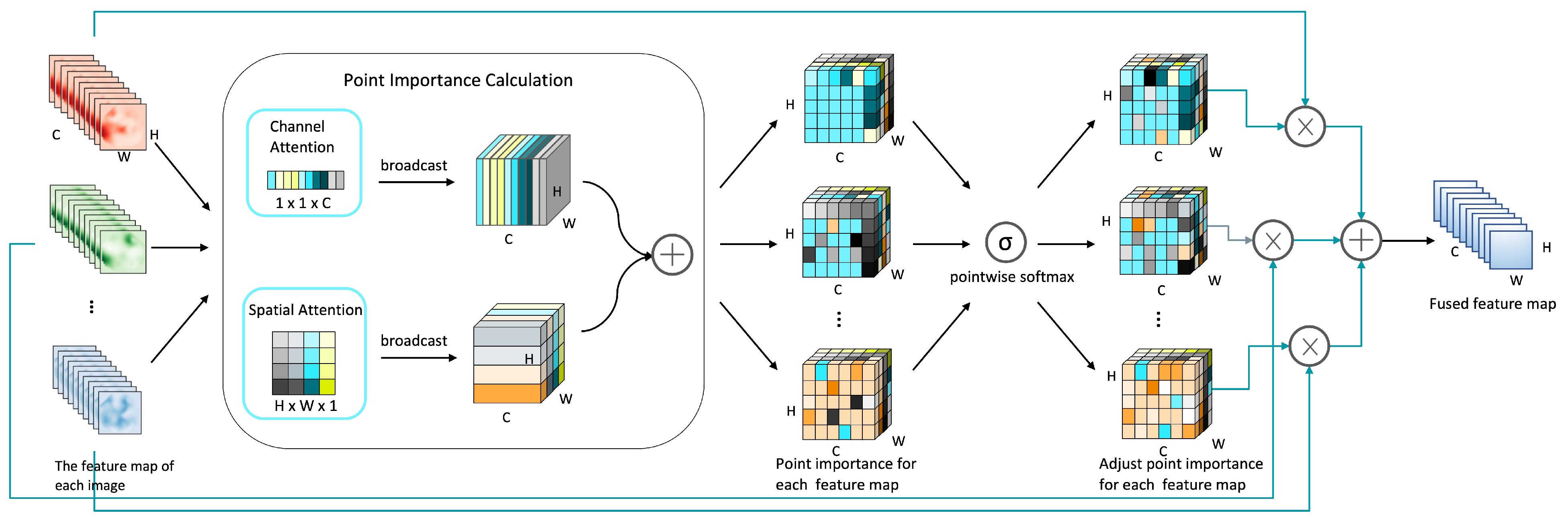
The feature map fusion module is proposed to solve the situation that the number of images collected in each CME event is not fixed. The illustration of the feature map fusion module is shown in Figure 3. When the deep residual network embedded with the attention mechanism extracts the feature map for each input image in the CME event, the feature map fusion module fuses the feature map of each image into a fused feature map based on the attention mechanism. It can be divided into three steps:
- Calculate the importance of each point in the feature map based on the attention mechanism. The module attention mechanism can focus limited attention on important regions. Through the above-mentioned channel attention module and spatial attention module, the feature map attention weights of the different channels axes and spatial axes are obtained, then the two attention weights are combined by adding to obtain the each point importance of the feature map.
- Adjust the point importance of each feature map in combination with the mutual influence between the time series feature maps. If there are N feature maps, for each point coordinate of the ith feature map, it will adjust its weight through the weight of the same position in other feature maps as follows:where represents the importance of the point whose coordinates of the j feature map is . Here, assuming that the shape of the feature map is , then , , .
- Fuse all feature map weights and point importances into one feature map. We multiply the point importance of each feature map with the original feature map weights to obtain the contribution of each feature map in the final fused feature map, and add the contribution of each feature map to get a fused feature map.
2.2. Arrival Time Prediction for Geoeffective CMEs
2.2.1. Data Expansion Based on Sample Split
The well performance of deep learning is inseparable from large-scale training data. In the prediction of the arrival time for geoeffective CME events, there are only 246 geoeffective CME events, and the number of observation images in each CME event is not fixed. The small sample size of the geoeffective CME events and the complexity of each sample make it difficult for the regression network to learn distinguishing features.
Since each observation image in the CME event can obtain its corresponding transit time by subtracting the observation time from the arrival time of the CME event, we can split the CME event to expand the scale of the data. Specifically, we split each observation image collected in the CME events as a new sample and use the transit time of the corresponding image as the label. For each image, our network predicts its transit time. After that, the sample size can be increased to 10×, and from the original 246 samples to the current 3460 samples. In the training phase, the network predicts the transit time of each observation image, and the predicted arrival time can be obtained by adding the transit time to the observation time of the image. In the testing phase, we calculate the average arrival time of each input image in this CME event as the arrival time of this CME event.
2.2.2. Deep Residual Regression Network Based on Group Convolution
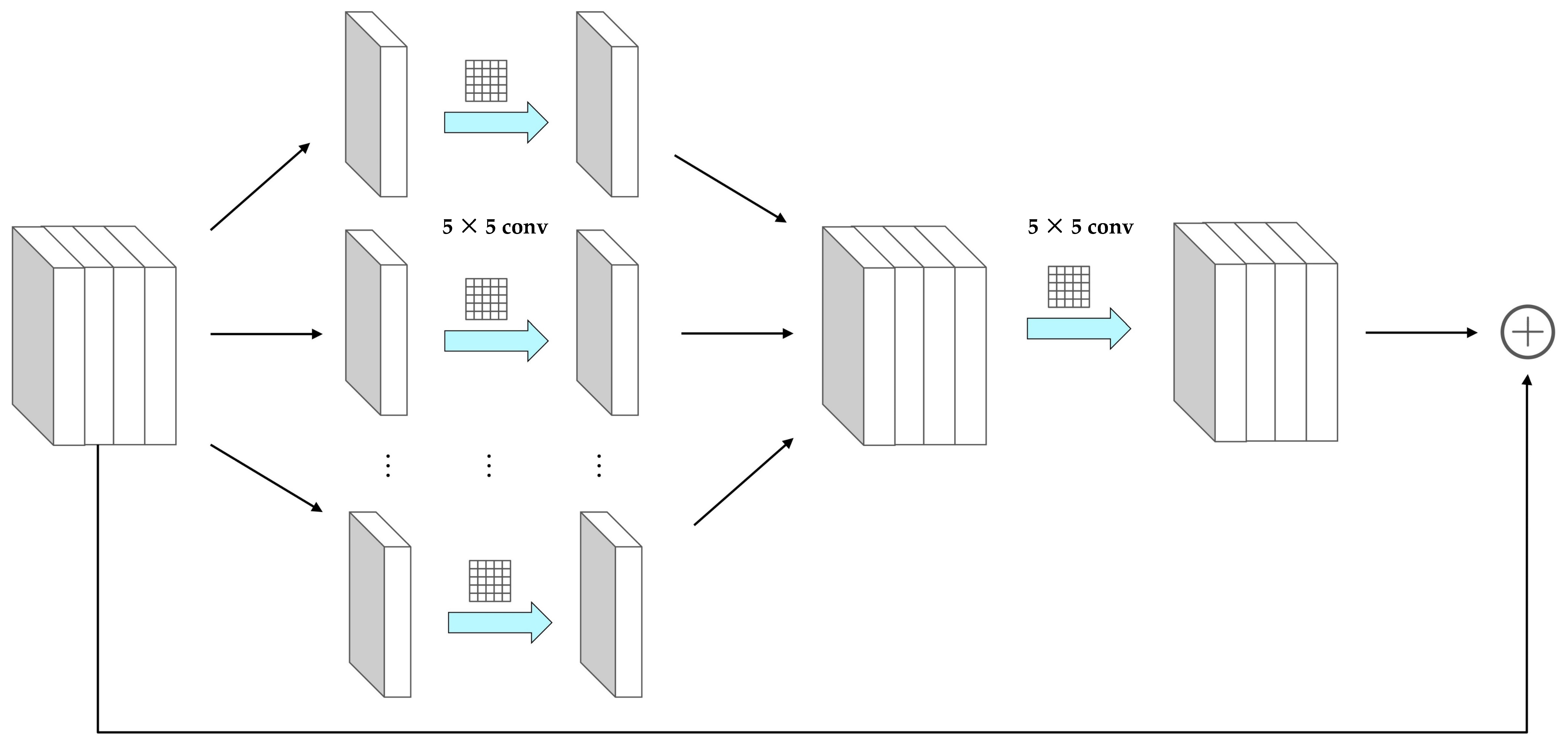
The architecture of the arrival time prediction network is shown in Table 2. The overall architecture is similar to the geoeffectiveness feature extraction network. First, through the data preprocessing, the original image is scaled, normalized and gray-scale processed in sequence. The first two layers of the network still use the same convolutional layer and max pooling. Next layers are composed of six residual blocks based on group convolution, and the illustration of the residual block is shown in Figure 4. Referring to the idea of Resnext [31], the network introduces group convolution to realize the split-transform-merge strategy. Through group convolution, the floating point operations (FLOPs) of the network can be reduced while increasing the cardinality of the network to improve the performance of the network.
The residual blocks based on group convolution first splits the input feature map in the channel dimension to obtain sub-feature maps, where is a parameter and uses as the default value of 32 in our network. The shape of each sub-feature map is . Next, convolution operation with the filter size of is performed on each sub-feature map to transform and learn the features of each sub-feature map. Then the transformed sub-feature maps are reconnected in the channel dimension, and the information of the inter sub-feature maps is merged through the convolution operation. Finally, the merged feature map is added with the shallow input feature maps. There are two purposes using residual connection based on group convolution. One is reducing the FLOPs of the network and speeding up the network. If the parameter of group convolution is , the FLOPs of group convolution is only of traditional convolution operation. The other is increasing the cardinality of the network. In addition to the dimensions of depth and width, cardinality is also an essential factor that can improve the performance of the network.
After extracting the feature map from the input image, the multi-layer perceptron module is followed to obtain the predicted arrival time, which contains two fully connected layers and Dropout [46]. The random inactivation probability of Dropout is 0.2 to prevent the network from overfitting.
2.2.3. Cost-Sensitive Regression Loss Function
In the training phase, each observed image uses the deep residual regression network based on group convolution to predict the transit time. But we find that the loss between different images is quite different. We hope that the network can focus more attention on hard samples and reduce the proportion of simple samples in the loss function. In this paper, we propose a cost-sensitive regression loss function through the combination of L1 Loss and L2 Loss. The formula is as follows:
where represents the prediction result of our network, represents the actual label, and is manually set as a positive number greater than 1. We define the sample with an error less than or equal to as an easy sample, and the sample with an error greater than as a hard sample. In the training phase, the error of almost all samples is greater than 1. For these easy samples with a loss greater than 1, using L1 Loss can reduce its proportion in the loss function, and when the gradient is updated by backpropagation [47], the absolute value of the gradient contributed by these easy samples is only 1, which reduces the impact on the network. For hard samples, the value of the loss function is much larger than easy samples, thus avoiding the situation where the loss function is dominated by easy samples. Meanwhile, the absolute value of the gradient contributed during backpropagation is greater than , which is also much larger than the simple sample, and the greater the error, the greater the absolute value of the gradient. Compared with L1 Loss, our loss distinguishes samples with different errors on the gradient of backpropagation. Compared with L2 Loss, our loss reduces the proportion of most easy samples in the loss function and the contribution of gradient updates, so that the network can pay more attention to hard samples.
3. Experiments
3.1. Dataset
The performance of a deep learning algorithm is inseparable from large-scale data, so we collect partial-/full-halo CME events and corresponding satellite time series observation images from 1996 to 2018 to build a large-scale and differentiated data set.
First, we select partial-/full-halo CME events from the SOHO LASCO CME Catalog [48], and each CME event includes onset time, the angular width and other parameters. Then the geoeffectiveness of each CME event is checked with other sources’ data. The geoeffectiveness definition used in this research is one CME eventually arrives at Earth and causes geomagnetic disturbances during which the minimal Dst index is smaller than −30 nT. We employ a similar approach to the one in CAT-PUMA [21] to construct the geoeffective CMEs data set, collect events from the Richardson and Cane List [49], the full halo CMEs provide by the University of Science and Technology of China [50], the George Mason University CME/ICME List [51] and the CME Scoreboard by NASA, respectively. We collect geoeffective CMEs and their corresponding onset/arrival time. Here the onset time is the time of a CME’s first appearance in the Field-of-View (FOV) of SOHO LASCO C2, and the arrival time of CMEs is defined as the arrival time of interplanetary shocks driven by CMEs hereafter. After that, align the collected geoeffective CMEs with the selected partial-/full-halo CME events through onset time.
For convenience, we collected images directly through CDAW Data Center (https://cdaw.gsfc.nasa.gov/images/soho/lasco/ (accessed on 18 March 2021), the Day Month Year can be obtained through the corresponding CME event). Observations from Extreme ultraviolet Imaging Telescope (EIT) on the SOHO spacecraft or Atmospheric Imaging Assembly (AIA) on the Solar Dynamics Observatory (SDO) can provide some information on the source region of CMEs, while the LASCO C2 coronagraph observations provide CMEs’ evolution and propagation information. So for each CME event, the composite running-difference images of SOHO/LASCO C2 and SOHO/EIT or SDO/AIA from 10 min before up to 4 h after the onset times of the events are collected. We believe such combined observations are more discriminative and can provide a better forecast.
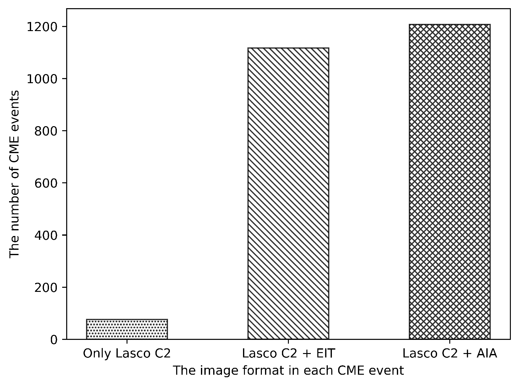
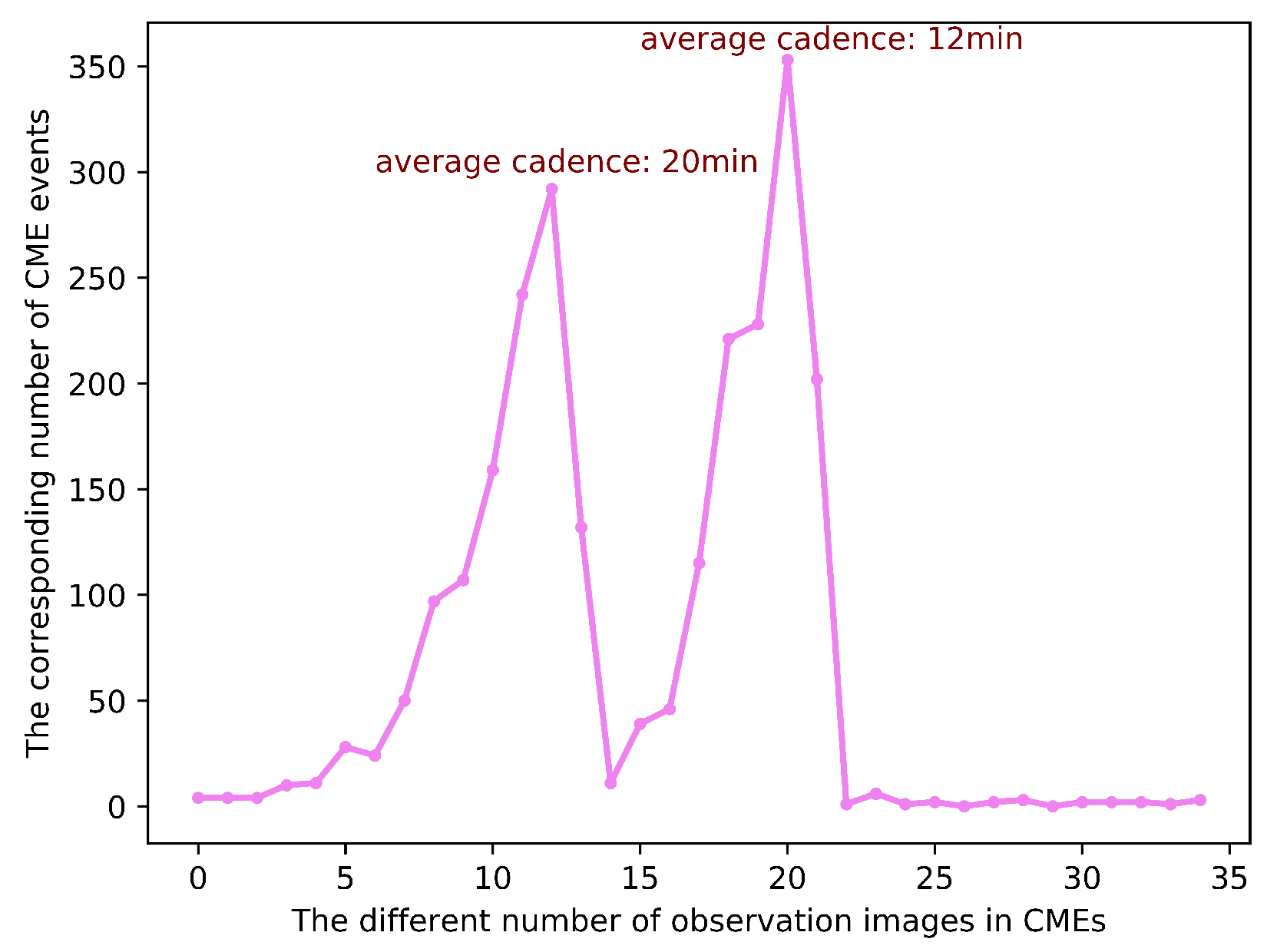
After the CME events with zero images are eliminated, there are a total of 2400 partial-/full-halo CME events and corresponding 35,666 images are collected, including 246 geoeffective CME events and 3460 corresponding images. In our data set, since the SDO satellite was launched in 2010 and the CCD bakeout of EIT and AIA, there will be three different formats of observations images: only LASCO C2 format, LASCO C2 combine EIT format and LASCO C2 combine AIA format. Meanwhile, we count the distribution of images in the CME events, as indicated in Figure 5, the number of CME events with only LASCO C2 format is 76, the number of CME events with LASCO C2 combine EIT format is 1117 and the number of CME events with LASCO C2 combine AIA format is 1207. The CME events which only contain LASCO C2 observation are fewer and randomly distributed in geoeffective or non-geoeffective CMEs, so they will not bias the training and testing of our method. Due to the different operation status of different instruments, the time interval between adjacent observation images is not fixed, which will lead to large fluctuations in the number of images collected for each CME event (shown in Figure 6).
3.2. Experimental Setting
In order to train and evaluate the proposed deep learning framework, we introduce the experimental setting.
For the geoeffectiveness prediction of CMEs, 2400 CME events are randomly divided into the training set and the testing at approximately 4:1 ratio, and the proportion of geoeffective and non-geoeffective samples in the training set is basically the same as that in the testing set. Specifically, the training set has 1725 non-geoeffective samples and 197 geoeffective samples, and the testing set has 429 non-geoeffective samples and 49 geoeffective samples. The training procedure is performed in the PyTorch framework. In the training phase, we use Adam [52] as the default optimizer to update the parameters of all deep learning methods in which the learning rate is 0.001, the related parameters and are set to 0.9 and 0.999. One hundred epochs are used for training, and the batch size is 1. The training of all methods adopts a down-sampling strategy due to the imbalanced geoeffective and non-geoeffective samples. Specifically, one eighth of the non-geoeffective samples are combined with the geoeffective samples as the training samples in each epoch. The loss function adopts binary cross-entropy, the formula is as follows:
where represents the actual label of the ith sample, when the current sample is geoeffective, the corresponding value of is 1, otherwise it is 0, represents the probability that the ith sample is predicted to be a geoeffective, and N represents the number of samples.
For the arrival time prediction of geoeffective CMEs, 246 geoeffective CME events are randomly divided into the training set and the testing set at approximately 8:1 ratio. Specifically, the training set contains 218 CME events and corresponding 3042 observation images while the testing set contains 28 CME events and corresponding 418 observation images. The training procedure is also performed in the PyTorch framework. In the training phase, we use AdamW as the default optimizer to update the parameters and avoid the network overfitting, the related parameters and are also set to 0.9 and 0.999, the weight decay coefficient is set to 0.01. We train with a total number of 100 epochs and the default batch size is 32. The learning rate is set to 0.01 initially, and is multiplied by 0.6 at epoch 40, 60 and 80. The comparing traditional convolutional neural networks all adopt L2 Loss and data expansion based on sample split in the training phase.
4. Results
4.1. Results on the Geoeffectiveness Prediction of CMEs
To assess the performance of the geoeffectiveness prediction algorithm, we divide the data into four types based on the prediction results and actual label. Record the CME events that are geoeffective and correctly predicted as true positive (TP), the CME events that are non-geoeffective and correctly predicted as true negative (TN), the CME events that are geoeffective but incorrectly predicted as false negative(FN), the CME events that are non-geoeffective but incorrectly predicted as true negative (FP). Based on the four types of classification results, the metrics for evaluating the prediction of geoeffectiveness algorithm can be obtained through the following formulas:
Accuracy is a widely used metric that measures the performance of a classifier and the definition is the percentage of the correctly classified positive and negative examples. F1 score is the trade-off recall and precision. Precision is the fraction classified as geoeffective CMEs that are true geoeffective CMEs and its value is equal to , recall is the fraction of true geoeffective CMEs recovered by the model and its value is equal to . Due to the imbalance of geoeffective and non-geoeffective samples, F1 score is a better choice metric [53]. And we use F1 score as the main evaluation metric, and Accuracy as the secondary evaluation metric. The performance of different models is first compared with the F1 score, and when the F1 score is the same, the Accuracy is further compared. The two metrics both need a threshold for deciding when the model output in the range [0, 1] becomes a positive class and we use 0.5 as the default parameter.
We first compare the proposed geoeffectiveness prediction method with traditional convolutional neural networks (CNNs), including VGG [27], Resnet [28], MobileNetv2 [54]. VGG increases the depth of the network by stacking convolution filters, Resnet introduces residual learning to train the deeper neural networks, MobileNetv2 introduces inverted residual structure on the basis of depthwise separable convolution. The results are shown in Table 3, our method has significant improvement in F1 score and accuracy, with an average improvement of 0.041 and 11.8%, respectively. The main reasons are as follows—firstly, the kernel size of the convolution filter of the traditional CNNs is relatively small, which is not fit well for the sparse features of the CME observation image; secondly, the attention mechanism in residual blocks of our network can distinguish the features of different regions by different attention weights; thirdly, these traditional CNNs fuse the feature maps of different observation images by simply averaging the feature maps which may cause the role of the important feature map is downplayed.
Then, we compare the method of long short-term memory (LSTM) [55] combined with CNN, which extracts the features of each image through CNN and uses LSTM to combine time series features, but the result is not good. The main reasons are as follows—one is that the time interval between adjacent observation images is large, and it leads to the relationship between time series images become difficult to capture; the other is the number of time series observation images in each CME event is unfixed, it increases the training difficulty of LSTM combined with CNN.
In summary, the deep residual network embedded with the attention mechanism and the feature map fusion module proposed in this paper are effective and the performance of our method is significantly better than traditional deep learning methods.
4.2. Results on the Arrival Time Prediction for Geoeffective CMEs
On the arrival time prediction of CME events, the evaluation metric adopts mean absolute error (MAE). The MAE formula can be defined as follows:
where N represents the number of CME events in the testing set, represents the actual arrival time of the ith CME event, and represents the predicted arrival time.
For comparison with other methods, we chose four well-known CNN models and three machine learning/deep learning methods, which are used in the CME arrival time prediction task. The results are shown in Table 4.
In addition to the three CNN models mentioned above, we also add ResNext [31] to compare. Resnext repeats a building block that aggregates a set of transformations with the same topology. The mean absolute error of four CNN models is 8.1 h and has been increased 2.3 h in average when compared to our method. The main reasons for the better performance of our method are as follows—firstly, our method uses a more suitable kernel size of the convolution filter; secondly, our method introduces the residual block based on group convolution to train deeper networks and improve network performance by increasing the cardinality of the network; thirdly, our method uses cost-sensitive regression loss function to reduce the error of hard sample.
Meanwhile, we also compare with the machine learning/deep learning methods used in CME arrival time prediction. Sudar et al. [20] uses FCNN to predict the transit time for CME events using the initial velocity of the CME and the central meridian distance of the associated flare as inputs, the MAE is about 11.6 h and is twice the error of our method. CAT-PUMA [21] uses SVM fitting parameters to predict the arrival time for geoeffective partial-/full-halo CME events, the MAE is increased 0.1 h when compared with our method. Moreover, 5.9 h is the best result in a random 100,000 testing set. Both two machine learning methods are necessary to manually collect the parameters and if the relevant parameters are missed, errors of the related CME events will be raised. Wang et al. [23] first uses CNN to predict the arrival time for geoeffective CME events, with an error of 12.4 h. Compared with our method, the error is greatly increased. The main reason is that the network is too simple to capture distinguishing features, and it only uses the observation of the LASCO C2 white light coronagraph as input.
Finally, we determine the value of in the cost-sensitive regression loss function through enumeration on the basis of data expansion and deep residual regression network. As shown in Table 5, the MAE is 6.4 h when using L2 Loss. After switching to cost-sensitive regression loss, different all bring a small improvement, with an average improvement of 0.3 h. Among them, the value of 3 is the optimal choice and the MAE is only 5.8 h.
In summary, our proposed arrival time prediction algorithm is effective and is better than well-known machine learning/deep learning methods.
5. Discussion
Time series of solar white-light running-difference images can be used to extract the morphology features of CMEs by tracking the bright structure in the coronagraph FOV [56]. EUV images of the whole solar disk provide information on CMEs’ source regions with additional spatial and temporal coverage in eruption observations. Taking combinations of both observation images as input, our deep learning framework outperforms the state-of-the-art methods both on the geoeffectiveness and arrival time prediction of the CME events (see experimental results given in Section 4). Besides, it has the following features:
- This is the first time that making geoeffectiveness and arrival time prediction of CMEs in a unified deep learning framework.
- This is the first time that the CNN method is applied to geoeffectiveness prediction of CMEs.
- The only input of the deep learning framework is the time series images from synchronized solar white-light and EUV observation images that are directly observed.
- Once we get the observation images, we can immediately get the prediction result with no requirement of manually feature selection and professional knowledge.
5.1. Discussion on the Prediction of Geoeffectiveness
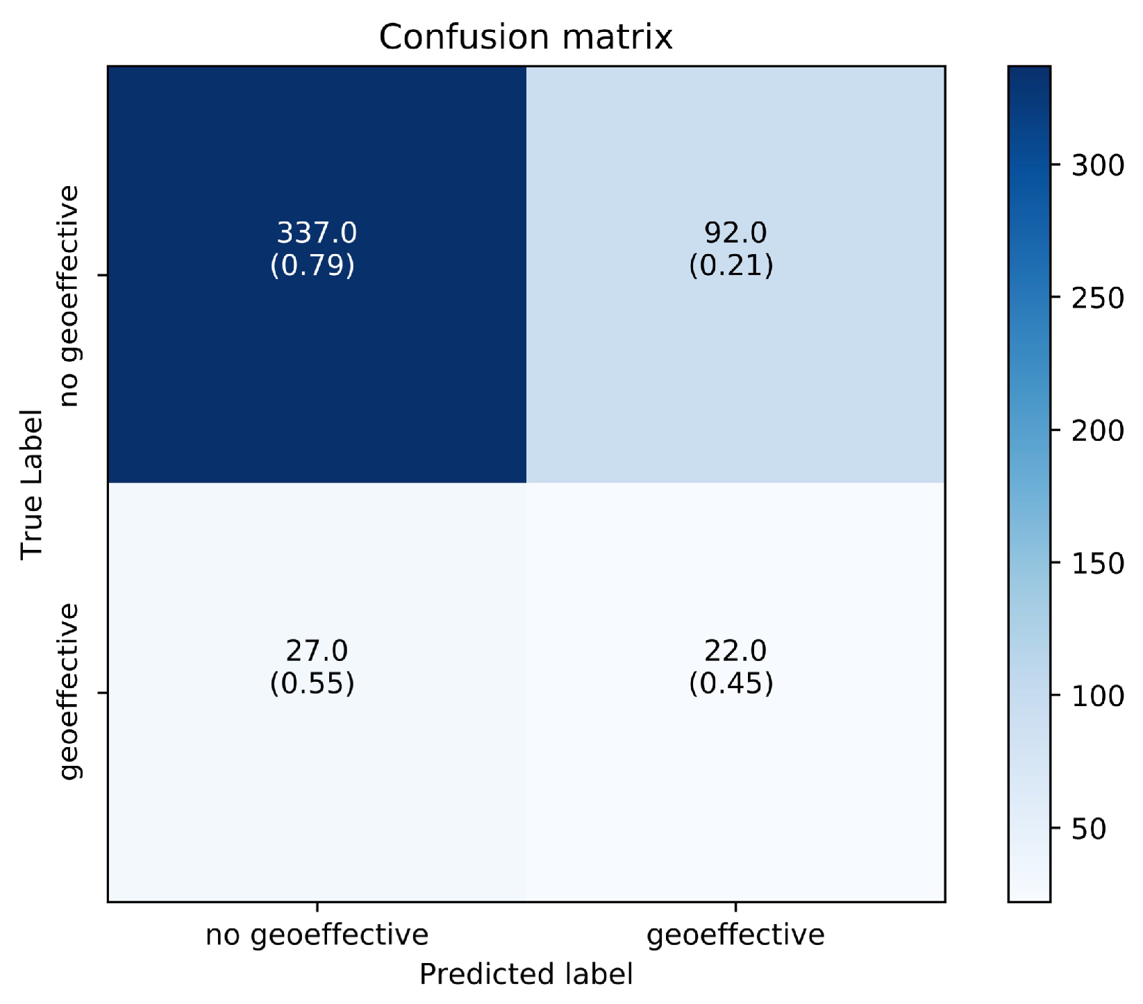
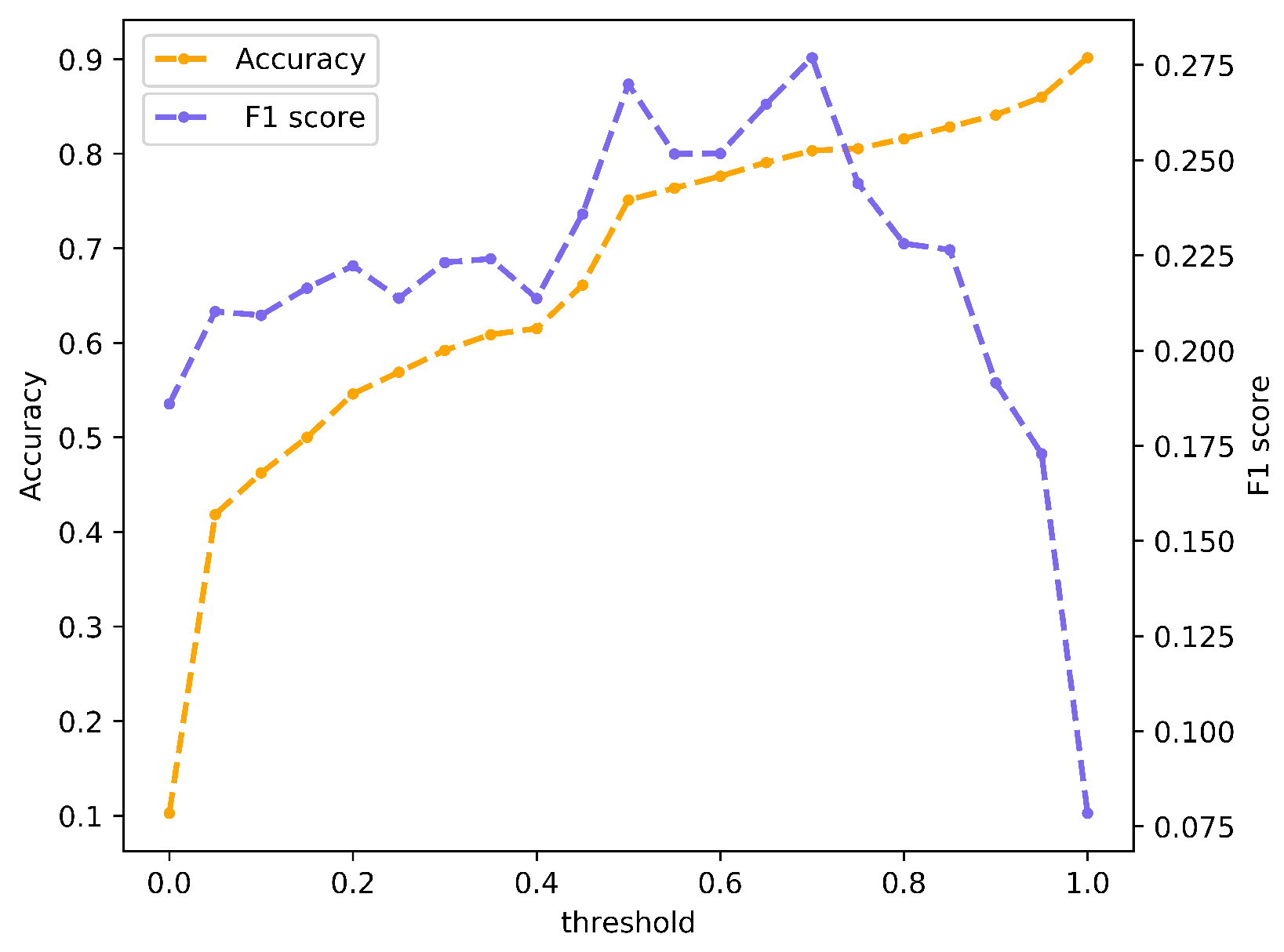
The previous experimental results show that our method is effective for geoeffectiveness prediction. But there are still many misjudgments, we discuss the main source of classification error through the confusion matrix on the testing set. As shown in Figure 7, our method predicts the CME events that are non-geoeffective as geoeffective and 92 CME events are misclassified. This may be caused by the choice of the threshold, therefore the performance of our method under different thresholds is analyzed. As shown in Figure 8, we select 20 thresholds at equal intervals between [0, 1] to verify the performance of the method. When the threshold is changed from the default 0.5 to 0.7, we get a higher F1 score and Accuracy, and they are 0.277% and 80.3%, respectively. The main reason is that the threshold is changed from 0.5 to 0.7, the number of CME events incorrectly predicted as geoeffective has greatly decreased while the number of CME events that correctly predicted as geoeffective is almost unchanged. However, with the threshold continues to increase, almost all CMEs are predicted as non-geoeffective, and due to the imbalance of samples in the test set, samples that are non-geoeffective account for about 90%, so the Accuracy is still continue to improve but F1 score has reduced sharply. This phenomenon also reflects the rationality of our evaluation metrics. For unbalanced data, F1 score can better reflect the performance of the model. When the F1 score of two methods is the same, we can distinguish through Accuracy. In the practical applications, we also can select different thresholds according to the actual needs.
5.2. Discussion on the Arrival Time Prediction for Geoeffective CMEs
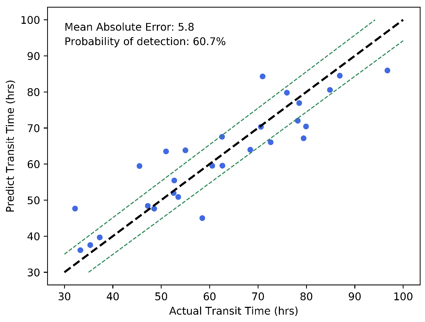
Here, we first discuss the relationship between the predicted transit time of our method and the actual transit time on the testing set. As shown in Figure 9, the different blue dots represent the different CME events. The black dashed line representing the predicted transit time is equal to the actual transit time. The two green dashed lines show the deviation from the black line and the deviation is 5.8 h, which represents the MAE of our method. From the distribution of the dots, we can find that most dots are between the two green dashed lines and the dots are scattered close to the black dashed line. This proves that our method is effective for most CME events, and the prediction error of most CME events is less than 5.8 h. Specifically, we use the probability of detection (POD) to quantify the probability that the CME prediction error is less than the MAE of our method, and the formula is defined as follows:
where the absolute prediction errors less than 5.8 h are called Hits and others called Misses. The POD of our method is 60.7%.
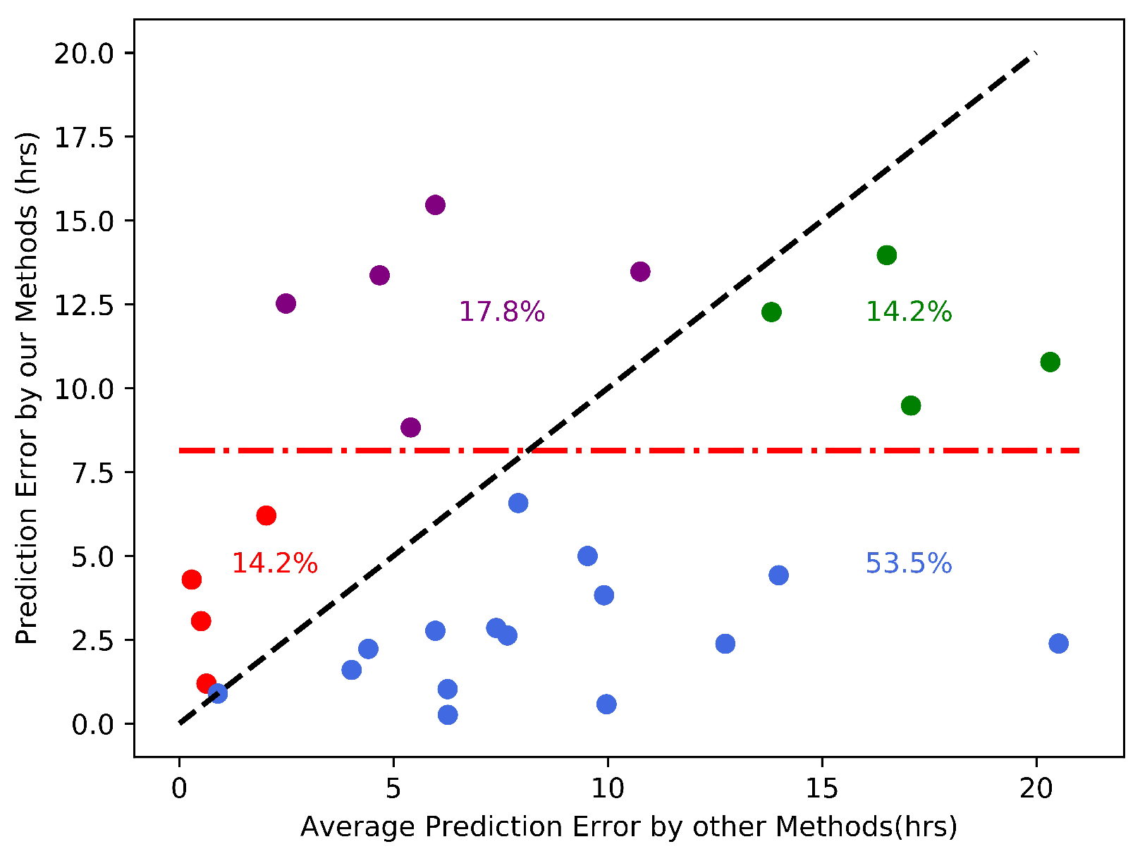
Then, we discuss the detailed comparison of our method for CMEs in the testing set with four well-known CNN models (VGG, Resnet, MobileNetv2, Resnext). As shown in Figure 10, the red dash-dotted line indicates the average absolute errors of CNN methods and its value is 8.1 h. The blue dots (53.5%) represent the events that our method has a better performance and the error is less than 8.1 h. The green dots (14.2%) represent the events that our method has a better performance but the error is greater than 8.1 h. The red dots (14.2%) represent the events that our method performs worse and the error is less than 8.1 h. The purple dots (17.8%) represent the events that our method performs worse and the error is greater than 8.1 h. In general, our method performs better for 67.7% CME events.
5.3. Applicability of the Proposed Framework in the Feature
When our method completes training and obtains the optimal weights, once we feed the observation images to the framework, we can immediately obtain the prediction results. In the future study, with the continuous high frequency of CME events, more CME events and corresponding satellite observation images will be collected, so the data set will be further expanded. As the size of the data set continues to increase, the performance of the model is expected to be further improved. Meanwhile, with the gradual implementation of new satellite observation projects, such as Advanced Space-Based Solar Observatory, continuous high-temporal-resolution images of solar observations will also improve the performance of our method.
6. Conclusions
In this paper, we propose a deep learning framework based on satellite time series observation images that can predict both the geoeffectiveness and the arrival time of CME events with no requirement for manually feature selection or professional knowledge. We construct a data set with 2400 partial-/full-halo CME events and 246 geoeffective partial-/full-halo CME events from 1996 to 2018. On the geoeffectiveness prediction of CME events, 2400 CME events are randomly divided into training set and testing set at approximately 4:1 ratio. On arrival time prediction of geoeffective CMEs, 246 geoeffective CME events are randomly divided into a training set and a testing set at approximately 8:1 ratio. Extensive experiments are conducted by comparing with state-of-the-art methods.
The main results of this study can be summarized as follows. First, the deep learning framework has been successfully applied to the geoeffectiveness and arrival time prediction of CME events. Second, on the geoeffectiveness prediction of CMEs, we propose a deep residual network embedded with the attention mechanism and the feature map fusion module to extract key regional features and fuse the features from each image. Third, data expansion method, deep residual regression network and cost-sensitive regression loss function are proposed to improve the performance of the arrival time prediction of CMEs. Fourth, our method is superior to other state-of-the-art deep learning methods on the geoeffectiveness prediction of CMEs, it can achieve 0.270 F1 score and 75.1% accuracy. Fifth, regarding arrival time prediction, our method is better than traditional CNNs and the machine learning/deep learning methods applied previously and the mean absolute error is only 5.8 h.
In this work, we have demonstrated the importance of satellite time series images. In the future, we will combine the parameter features such as the angular width, average speed, estimated mass, and so forth, with observation images for multimodal machine learning, and the features extracted from the image can be combined with other features to further improve the performance of the model. Furthermore, future work will introduce refined predictions to give a high-level priority to CMEs associated with stronger solar flares (i.e., M class or above flares) to reduce potential damages to the maximum.
Author Contributions
H.F. and Y.Z. jointly conceived the idea, performed the experiments and wrote the manuscript; Y.Z. and Y.Y. collected and analyzed the data. X.F., C.L. and H.M. supervised the study and reviewed this paper. All authors have read and agreed to the published version of the manuscript.
Funding
This research was funded by the National Natural Science Foundation of China under No.61872047 and No.61720106007, the 111 Project under No.B18008, the Funds for Creative Research Groups of China under No.61921003, and the Beijing Nova Program under No.Z201100006820124.
Institutional Review Board Statement
Not applicable.
Informed Consent Statement
Not applicable.
Data Availability Statement
Publicly available datasets in this study are described in Section 3.1, and the data can be obtained according to the described steps.
Acknowledgments
We are grateful to The SOHO LASCO CME catalog. The SOHO LASCO CME catalog is generated and maintained at the CDAW Data Center by NASA and The Catholic University of America in cooperation with the Naval Research Laboratory. SOHO is a project of international cooperation between ESA and NASA.
Conflicts of Interest
The authors declare no conflict of interest.
References
- Kataoka, R. Probability of occurrence of extreme magnetic storms. Space Weather 2013, 11, 214–218. [Google Scholar] [CrossRef]
- Gonzalez, W.D.; Tsurutani, B.T.; De Gonzalez, A.L.C. Interplanetary origin of geomagnetic storms. Space Sci. Rev. 1999, 88, 529–562. [Google Scholar] [CrossRef]
- Eastwood, J.; Biffis, E.; Hapgood, M.; Green, L.; Bisi, M.; Bentley, R.; Wicks, R.; McKinnell, L.A.; Gibbs, M.; Burnett, C. The economic impact of space weather: Where do we stand? Risk Anal. 2017, 37, 206–218. [Google Scholar] [CrossRef] [PubMed]
- Domingo, V.; Fleck, B.; Poland, A. SOHO: The solar and heliospheric observatory. Space Sci. Rev. 1995, 72, 81–84. [Google Scholar] [CrossRef]
- Gopalswamy, N.; Mäkelä, P.; Xie, H.; Yashiro, S. Testing the empirical shock arrival model using quadrature observations. Space Weather 2013, 11, 661–669. [Google Scholar] [CrossRef] [Green Version]
- Xie, H.; Ofman, L.; Lawrence, G. Cone model for halo CMEs: Application to space weather forecasting. J. Geophys. Res. Space Phys. 2004, 109. [Google Scholar] [CrossRef]
- Davies, J.; Harrison, R.; Perry, C.; Möstl, C.; Lugaz, N.; Rollett, T.; Davis, C.; Crothers, S.; Temmer, M.; Eyles, C.; et al. A self-similar expansion model for use in solar wind transient propagation studies. Astrophys. J. 2012, 750, 23. [Google Scholar] [CrossRef]
- Howard, T.; Nandy, D.; Koepke, A. Kinematic properties of solar coronal mass ejections: Correction for projection effects in spacecraft coronagraph measurements. J. Geophys. Res. Space Phys. 2008, 113, A01104. [Google Scholar] [CrossRef]
- Kaiser, M.L.; Kucera, T.; Davila, J.; Cyr, O.S.; Guhathakurta, M.; Christian, E. The STEREO mission: An introduction. Space Sci. Rev. 2008, 136, 5–16. [Google Scholar] [CrossRef]
- Howard, R.A.; Moses, J.; Vourlidas, A.; Newmark, J.; Socker, D.G.; Plunkett, S.P.; Korendyke, C.M.; Cook, J.; Hurley, A.; Davila, J.; et al. Sun Earth connection coronal and heliospheric investigation (SECCHI). Space Sci. Rev. 2008, 136, 67–115. [Google Scholar] [CrossRef] [Green Version]
- Möstl, C.; Isavnin, A.; Boakes, P.; Kilpua, E.; Davies, J.; Harrison, R.; Barnes, D.; Krupar, V.; Eastwood, J.; Good, S.; et al. Modeling observations of solar coronal mass ejections with heliospheric imagers verified with the Heliophysics System Observatory. Space Weather 2017, 15, 955–970. [Google Scholar] [CrossRef] [Green Version]
- Vršnak, B.; Žic, T.; Vrbanec, D.; Temmer, M.; Rollett, T.; Möstl, C.; Veronig, A.; Čalogović, J.; Dumbović, M.; Lulić, S.; et al. Propagation of interplanetary coronal mass ejections: The drag-based model. Sol. Phys. 2013, 285, 295–315. [Google Scholar] [CrossRef]
- Feng, X.; Zhao, X. A new prediction method for the arrival time of interplanetary shocks. Sol. Phys. 2006, 238, 167–186. [Google Scholar] [CrossRef]
- Corona-Romero, P.; Gonzalez-Esparza, J.; Aguilar-Rodriguez, E.; De-la Luz, V.; Mejia-Ambriz, J. Kinematics of ICMEs/shocks: Blast wave reconstruction using type-II emissions. Sol. Phys. 2015, 290, 2439–2454. [Google Scholar] [CrossRef] [Green Version]
- Feng, X.; Zhou, Y.; Wu, S. A novel numerical implementation for solar wind modeling by the modified conservation element/solution element method. Astrophys. J. 2007, 655, 1110. [Google Scholar] [CrossRef] [Green Version]
- Shen, F.; Feng, X.; Wu, S.; Xiang, C. Three-dimensional MHD simulation of CMEs in three-dimensional background solar wind with the self-consistent structure on the source surface as input: Numerical simulation of the January 1997 Sun-Earth connection event. J. Geophys. Res. Space Phys. 2007, 112. [Google Scholar] [CrossRef] [Green Version]
- Wold, A.M.; Mays, M.L.; Taktakishvili, A.; Jian, L.K.; Odstrcil, D.; MacNeice, P. Verification of real-time WSA- ENLIL+ Cone simulations of CME arrival-time at the CCMC from 2010 to 2016. J. Space Weather. Space Clim. 2018, 8, A17. [Google Scholar] [CrossRef] [Green Version]
- Tóth, G.; Sokolov, I.V.; Gombosi, T.I.; Chesney, D.R.; Clauer, C.R.; De Zeeuw, D.L.; Hansen, K.C.; Kane, K.J.; Manchester, W.B.; Oehmke, R.C.; et al. Space Weather Modeling Framework: A new tool for the space science community. J. Geophys. Res. Space Phys. 2005, 110. [Google Scholar] [CrossRef] [Green Version]
- Besliu-Ionescu, D.; Talpeanu, D.C.; Mierla, M.; Muntean, G.M. On the prediction of geoeffectiveness of CMEs during the ascending phase of SC24 using a logistic regression method. J. Atmos. Sol. Terr. Phys. 2019, 193, 105036. [Google Scholar] [CrossRef]
- Sudar, D.; Vršnak, B.; Dumbović, M. Predicting coronal mass ejections transit times to Earth with neural network. Mon. Not. R. Astron. Soc. 2015, 456, 1542–1548. [Google Scholar] [CrossRef] [Green Version]
- Liu, J.; Ye, Y.; Shen, C.; Wang, Y.; Erdélyi, R. A new tool for CME arrival time prediction using machine learning algorithms: CAT-PUMA. Astrophys. J. 2018, 855, 109. [Google Scholar] [CrossRef] [Green Version]
- Smola, A.J.; Schölkopf, B. A tutorial on support vector regression. Stat. Comput. 2004, 14, 199–222. [Google Scholar] [CrossRef] [Green Version]
- Wang, Y.; Liu, J.; Jiang, Y.; Erdélyi, R. CME Arrival Time Prediction Using Convolutional Neural Network. Astrophys. J. 2019, 881, 15. [Google Scholar] [CrossRef] [Green Version]
- Deng, J.; Dong, W.; Socher, R.; Li, L.J.; Li, K.; Fei-Fei, L. Imagenet: A large-scale hierarchical image database. In Proceedings of the 2009 IEEE Conference on Computer Vision and Pattern Recognition, Miami, FL, USA, 20–25 June 2009; pp. 248–255. [Google Scholar]
- Lin, T.Y.; Maire, M.; Belongie, S.; Hays, J.; Perona, P.; Ramanan, D.; Dollár, P.; Zitnick, C.L. Microsoft coco: Common objects in context. In European Conference on Computer Vision; Springer: Berlin/Heidelberg, Germany, 2014; pp. 740–755. [Google Scholar]
- Krizhevsky, A.; Sutskever, I.; Hinton, G.E. Imagenet classification with deep convolutional neural networks. Adv. Neural Inf. Process. Syst. 2012, 25, 1097–1105. [Google Scholar] [CrossRef]
- Simonyan, K.; Zisserman, A. Very deep convolutional networks for large-scale image recognition. arXiv 2014, arXiv:1409.1556. [Google Scholar]
- He, K.; Zhang, X.; Ren, S.; Sun, J. Deep residual learning for image recognition. In Proceedings of the IEEE Conference on Computer Vision and Pattern Recognition, Las Vegas, NV, USA, 27–30 June 2016; pp. 770–778. [Google Scholar]
- Szegedy, C.; Liu, W.; Jia, Y.; Sermanet, P.; Reed, S.; Anguelov, D.; Erhan, D.; Vanhoucke, V.; Rabinovich, A. Going deeper with convolutions. In Proceedings of the IEEE Conference on Computer Vision and Pattern Recognition, Boston, MA, USA, 7–12 June 2015; pp. 1–9. [Google Scholar]
- Iandola, F.N.; Han, S.; Moskewicz, M.W.; Ashraf, K.; Dally, W.J.; Keutzer, K. SqueezeNet: AlexNet-level accuracy with 50× fewer parameters and <0.5 MB model size. arXiv 2016, arXiv:1602.07360. [Google Scholar]
- Xie, S.; Girshick, R.; Dollár, P.; Tu, Z.; He, K. Aggregated residual transformations for deep neural networks. In Proceedings of the IEEE Conference on Computer Vision and Pattern Recognition, Honolulu, HI, USA, 21–26 July 2017; pp. 1492–1500. [Google Scholar]
- Howard, A.G.; Zhu, M.; Chen, B.; Kalenichenko, D.; Wang, W.; Weyand, T.; Andreetto, M.; Adam, H. Mobilenets: Efficient convolutional neural networks for mobile vision applications. arXiv 2017, arXiv:1704.04861. [Google Scholar]
- Chollet, F. Xception: Deep learning with depthwise separable convolutions. In Proceedings of the IEEE Conference on Computer Vision and Pattern Recognition, Honolulu, HI, USA, 21–26 July 2017; pp. 1251–1258. [Google Scholar]
- Huang, G.; Liu, Z.; Van Der Maaten, L.; Weinberger, K.Q. Densely connected convolutional networks. In Proceedings of the IEEE Conference on Computer Vision and Pattern Recognition, Honolulu, HI, USA, 21–26 July 2017; pp. 4700–4708. [Google Scholar]
- Tan, M.; Le, Q. Efficientnet: Rethinking model scaling for convolutional neural networks. In Proceedings of the International Conference on Machine Learning, PMLR, Long Beach, CA, USA, 15–20 June 2019; pp. 6105–6114. [Google Scholar]
- Balduzzi, D.; Frean, M.; Leary, L.; Lewis, J.; Ma, K.W.D.; McWilliams, B. The shattered gradients problem: If resnets are the answer, then what is the question? In Proceedings of the International Conference on Machine Learning, PMLR, Sydney, Australia, 6–11 August 2017; pp. 342–350. [Google Scholar]
- Ioffe, S.; Szegedy, C. Batch normalization: Accelerating deep network training by reducing internal covariate shift. In Proceedings of the International Conference on Machine Learning, PMLR, Lille, France, 6–11 July 2015; pp. 448–456. [Google Scholar]
- Nair, V.; Hinton, G.E. Rectified linear units improve restricted boltzmann machines. In Proceedings of the International Conference on Machine Learning, PMLR, Haifa, Israel, 21–24 June 2010; pp. 807–814. [Google Scholar]
- Woo, S.; Park, J.; Lee, J.Y.; Kweon, I.S. Cbam: Convolutional block attention module. In Proceedings of the European Conference on Computer Vision (ECCV), Munich, Germany, 8–14 September 2018; pp. 3–19. [Google Scholar]
- Hu, J.; Shen, L.; Sun, G. Squeeze-and-excitation networks. In Proceedings of the IEEE Conference on Computer Vision and Pattern Recognition, Salt Lake City, UT, USA, 18–23 June 2018; pp. 7132–7141. [Google Scholar]
- Wang, X.; Girshick, R.; Gupta, A.; He, K. Non-local neural networks. In Proceedings of the IEEE Conference on Computer Vision and Pattern Recognition, Salt Lake City, UT, USA, 18–23 June 2018; pp. 7794–7803. [Google Scholar]
- Roy, A.G.; Navab, N.; Wachinger, C. Concurrent spatial and channel ‘squeeze & excitation’ in fully convolutional networks. In Proceedings of the International Conference on Medical Image Computing and Computer-Assisted Intervention, Granada, Spain, 16–20 September 2018; Springer: Berlin/Heidelberg, Germany, 2018; pp. 421–429. [Google Scholar]
- Fu, J.; Liu, J.; Tian, H.; Li, Y.; Bao, Y.; Fang, Z.; Lu, H. Dual attention network for scene segmentation. In Proceedings of the IEEE/CVF Conference on Computer Vision and Pattern Recognition, Long Beach, CA, USA, 15–20 June 2019; pp. 3146–3154. [Google Scholar]
- Li, X.; Wang, W.; Hu, X.; Yang, J. Selective kernel networks. In Proceedings of the IEEE/CVF Conference on Computer Vision and Pattern Recognition, Long Beach, CA, USA, 15–20 June 2019; pp. 510–519. [Google Scholar]
- Yang, Q.L.Z.Y.B. SA-Net: Shuffle Attention for Deep Convolutional Neural Networks. arXiv 2021, arXiv:2102.00240. [Google Scholar]
- Srivastava, N.; Hinton, G.; Krizhevsky, A.; Sutskever, I.; Salakhutdinov, R. Dropout: A simple way to prevent neural networks from overfitting. J. Mach. Learn. Res. 2014, 15, 1929–1958. [Google Scholar]
- Rumelhart, D.E.; Hinton, G.E.; Williams, R.J. Learning representations by back-propagating errors. Nature 1986, 323, 533–536. [Google Scholar] [CrossRef]
- Gopalswamy, N.; Yashiro, S.; Michalek, G.; Stenborg, G.; Vourlidas, A.; Freeland, S.; Howard, R. The soho/lasco cme catalog. Earth Moon Planets 2009, 104, 295–313. [Google Scholar] [CrossRef]
- Richardson, I.G.; Cane, H.V. Near-Earth interplanetary coronal mass ejections during solar cycle 23 (1996–2009): Catalog and summary of properties. Sol. Phys. 2010, 264, 189–237. [Google Scholar] [CrossRef]
- Shen, C.; Wang, Y.; Pan, Z.; Zhang, M.; Ye, P.; Wang, S. Full halo coronal mass ejections: Do we need to correct the projection effect in terms of velocity? J. Geophys. Res. Space Phys. 2013, 118, 6858–6865. [Google Scholar] [CrossRef] [Green Version]
- Hess, P.; Zhang, J. A study of the Earth-affecting CMEs of Solar Cycle 24. Sol. Phys. 2017, 292, 1–20. [Google Scholar] [CrossRef]
- Kingma, D.P.; Ba, J. Adam: A method for stochastic optimization. arXiv 2014, arXiv:1412.6980. [Google Scholar]
- Jeni, L.A.; Cohn, J.F.; De La Torre, F. Facing imbalanced data–recommendations for the use of performance metrics. In Proceedings of the 2013 Humaine Association Conference on Affective Computing and Intelligent Interaction, Geneva, Switzerland, 2–5 September 2013; pp. 245–251. [Google Scholar]
- Sandler, M.; Howard, A.; Zhu, M.; Zhmoginov, A.; Chen, L.C. Mobilenetv2: Inverted residuals and linear bottlenecks. In Proceedings of the IEEE Conference on Computer Vision and Pattern Recognition, Salt Lake City, UT, USA, 18–23 June 2018; pp. 4510–4520. [Google Scholar]
- Hochreiter, S.; Schmidhuber, J. Long short-term memory. Neural Comput. 1997, 9, 1735–1780. [Google Scholar] [CrossRef] [PubMed]
- Qu, M.; Shih, F.Y.; Jing, J.; Wang, H. Automatic detection and classification of coronal mass ejections. Sol. Phys. 2006, 237, 419–431. [Google Scholar] [CrossRef]
Figure 1.
The overall deep learning framework of jointing geoeffectiveness and arrival time prediction. In the framework, we first predict the geoeffectiveness of CMEs and for geoeffective CMEs, we further predict the arrival time.
Figure 1.
The overall deep learning framework of jointing geoeffectiveness and arrival time prediction. In the framework, we first predict the geoeffectiveness of CMEs and for geoeffective CMEs, we further predict the arrival time.

Figure 2.
The illustration of the residual block with embedded attention. It combines residual learning with the attention mechanism.
Figure 2.
The illustration of the residual block with embedded attention. It combines residual learning with the attention mechanism.

Figure 3.
The illustration of the feature map fusion module. It fuses the feature map of each image into a fused feature map based on the attention mechanism.
Figure 3.
The illustration of the feature map fusion module. It fuses the feature map of each image into a fused feature map based on the attention mechanism.

Figure 4.
The illustration of the residual block based on group convolution.

Figure 5.
The distribution of different formats in CME events.

Figure 6.
The distribution of the number of observation images in CME events.

Figure 7.
The confusion matrix of the geoeffectiveness prediction results of our method on the testing set.
Figure 7.
The confusion matrix of the geoeffectiveness prediction results of our method on the testing set.

Figure 8.
The performance of our method in geoeffectiveness prediction with different thresholds on the testing set.
Figure 8.
The performance of our method in geoeffectiveness prediction with different thresholds on the testing set.

Figure 9.
The relationship between the predicted transit time and the actual transit time of our method on the testing set.
Figure 9.
The relationship between the predicted transit time and the actual transit time of our method on the testing set.

Figure 10.
Compared with other methods on the arrival time prediction for each CME event on the testing set.
Figure 10.
Compared with other methods on the arrival time prediction for each CME event on the testing set.


Table 1.
The architecture of the deep residual network embedded with the attention mechanism.
| Layer Name | Layer | Output Size |
|---|---|---|
| Conv1 | , 64, stride 1 | |
| Max Pool | , max pool, stride 2 | |
| Conv2_x | ||
| Conv3_x | ||
| Conv4_x |
Table 2.
The illustration of the deep residual regression network based on group convolution.
| Layer Name | Layer | Output Size |
|---|---|---|
| Conv1 | , 64, stride 1 | |
| Max Pool | , max pool, stride 2 | |
| Conv2_x | ||
| Conv3_x | ||
| Conv4_x | ||
| FC1 | FC, Dropout | |
| FC2 | FC |
Table 3.
Comparison of the geoeffectiveness prediction of CME events with other methods.
| Method | F1 Score | Accuracy | ||
|---|---|---|---|---|
| ResNet18 | 0.203 | 59.0% | % | |
| Vgg16 | 0.235 | 67.4% | % | |
| MobileNetv2 | 0.249 | 63.4% | % | |
| CNN+LSTM | 0.185 | 11.5% | % | |
| Ours | 0.270 | - | 75.1% | - |
Table 4.
Comparison of the arrival time prediction for geoeffective CMEs with other methods.
| Method | MAE (Hours) | ||
|---|---|---|---|
| Convolutional Neural Networks | ResNet18 | 7.6 | |
| Vgg16 | 8.6 | ||
| MobilenetV2 | 8.0 | ||
| ResNext | 8.3 | ||
| Machine learning/deep learning used in CME arrival time prediction | FCNN | 11.6 | |
| CAT-PUMA | 5.9 | ||
| Wang’s CNN | 12.4 | ||
| - | Ours | 5.8 | - |
Table 5.
The performance of different loss functions and different values of based on data expansion and deep residual regression network.
Table 5.
The performance of different loss functions and different values of based on data expansion and deep residual regression network.
| Loss | MAE (Hours) |
|---|---|
| L2 Loss | 6.4 |
| cost-sensitive regression loss with = 2 | 6.1 |
| cost-sensitive regression loss with = 3 | 5.8 |
| cost-sensitive regression loss with = 4 | 6.2 |
| cost-sensitive regression loss with = 4.5 | 6.1 |
Publisher’s Note: MDPI stays neutral with regard to jurisdictional claims in published maps and institutional affiliations. |
© 2021 by the authors. Licensee MDPI, Basel, Switzerland. This article is an open access article distributed under the terms and conditions of the Creative Commons Attribution (CC BY) license (https://creativecommons.org/licenses/by/4.0/).
Share and Cite
MDPI and ACS Style
Fu, H.; Zheng, Y.; Ye, Y.; Feng, X.; Liu, C.; Ma, H. Joint Geoeffectiveness and Arrival Time Prediction of CMEs by a Unified Deep Learning Framework. Remote Sens. 2021, 13, 1738. https://0-doi-org.brum.beds.ac.uk/10.3390/rs13091738
AMA Style
Fu H, Zheng Y, Ye Y, Feng X, Liu C, Ma H. Joint Geoeffectiveness and Arrival Time Prediction of CMEs by a Unified Deep Learning Framework. Remote Sensing. 2021; 13(9):1738. https://0-doi-org.brum.beds.ac.uk/10.3390/rs13091738
Chicago/Turabian StyleFu, Huiyuan, Yuchao Zheng, Yudong Ye, Xueshang Feng, Chaoxu Liu, and Huadong Ma. 2021. "Joint Geoeffectiveness and Arrival Time Prediction of CMEs by a Unified Deep Learning Framework" Remote Sensing 13, no. 9: 1738. https://0-doi-org.brum.beds.ac.uk/10.3390/rs13091738
Note that from the first issue of 2016, this journal uses article numbers instead of page numbers. See further details here.