1. Introduction
As the human population grows, so does the demand for water. Furthermore, adverse changes in the quality and quantity of water affected by anthropopressure are observed. Moreover, this problem is exacerbated by climate change. With it comes a risk of increased frequency of water shortages [
1]. One of the important sources of surface water resources are lakes. Their protection requires taking preventive measures. Particular emphasis should be put on the coastal zones of lakes, which are habitats that combine the features of land and water environments. They play an important role in limiting the negative impact of the catchment on the ecological status of surface water. The buffer capacity of a coastal zone depends on the hydromorphological features of the lake basin [
2,
3] and land use [
4]. This was reflected in the legal provisions of the Water Framework Directive of the European Parliament and the WFD Council (2000/60/EC [
5], according to which the hydromorphological assessment of lakes is one of the assessment components of the ecological status of surface water. According to Annex V of [
5], among the morphological characteristics of a lake, particular attention should be paid to parameters, such as the length and shape of the shoreline, the slope of the shore, and the presence of shoreline structures. These elements are dynamically transformed as a result of undulations, erosion and denudation of banks, changes in the range of the water table, and human activity [
6,
7]. Therefore, there is a need to test the existing and formulate new solutions allowing for quick registration of the progressive changes in the relief of coastal zones and for determination of the actual bathymetric digital elevation model (DEM). Meanwhile, when developing bathymetric plans, the greatest attention is paid to depicting the deepest zones of lakes. Bathymetric measurement methods are constantly being improved and innovative applications of existing devices are being developed [
8,
9,
10,
11]. The selection of the method depends on many factors and there is no consensus on universal techniques allowing for accurate and cost-effective bathymetric measurements of entire water bodies, including the delineation of water bodies’ borders.
This paper is methodical and concerns the acquisition of data for determining the extent of the coastal zone and digital modeling of the lake bottom. One of the methods of bathymetric measurement of deep and non-transparent water are echosounders. Measurements taken from a boat traveling along selected transects are determined and stored with the positions of the boat and the depth of the lake bottom. In order to create a DEM, the points measured by the echosounder are interpolated using standard algorithms [
12,
13]. Echosounders are commonly used in measurements in deep water, but in the case of shallow water, they have significant limitations [
14].
The limitations of echosounders are related to two very important issues: (1) the possibility of penetration of overgrown coastal zones from the boat, (2) the measurement depth range, which is a function of the boat’s draft and the position of the sensor itself. Additionally, significant limitations of echosounder measurements are the shape and extent of the water bodies shoreline, which affect both the sensor penetration ability and the boat reach area.
The question is, how can we avoid above mentioned limitations in shallow water bathymetry quantification. The method proposed in this work is the application of the ALS Airborne Laser Scanner LiDAR (Light Detection and Ranging) aircraft-based laser scanner RIEGLVQ-1560i-DW, which uses two laser beams: green and infrared. It is not a typical bathymetry scanner (ALB—Airborne LiDAR Bathymetry), which usually uses only a green laser [
15] for penetration the water column and reflecting off the bottom. The RIEGLVQ-1560i-DW uses a green laser beam to penetrate a column of water in relation to the infrared beam that is absorbed by the water surface [
16]. These wavelengths combination allows the acquisition of scan data of complementary information, thus delivering two independent reflectance distribution maps, one per laser wavelength. In this paper, we propose to use the green LiDAR scanner for mapping vegetation and waterbody shoreline of lakes, where the echosounder limitation is significant. Using a green laser scanner for bathymetry is not a completely new method. This kind of sensors where typically used for bathymetric measurements in high-transparency lagoons and open sea environments [
15,
16,
17,
18,
19,
20] and highly transparent rivers [
21,
22]. Several applications of LiDAR bathymetry for the European sea show potential of this technology being operational method for surveying shallow water of coastal zone [
20,
23]. Limitation effects caused by waves [
23,
24], water transparency [
24,
25], and algae development [
20,
26] have been noticed.
There are several dual channel LiDARS, which could be used operationally for bathymetric measurements. These are, e.g., the Teledyne Optech Titan [
27], CZMIL [
18], Leica Chiroptera [
28], and Riegl VQ880G [
29].
The practical use of dual channel LiDAR complementarily with sonar is not common and typically concerns the sea or ocean bottom. Examples of using LiDAR and sonar together are shown in the Litto3D survey [
30,
31]. The authors presented several applications of the complementary use of LiDAR and sonar for determination of the bottom relief of the sea, lagoons and estuaries. Although, the authors did not compare the methods presented. The interesting work done for the shallow sea depth inspired us to investigate the potential of this technique for mapping the littoral zone of inland lakes. To the knowledge of the authors, there are no published Green LiDAR applications for the investigation of lake’s shore zone.
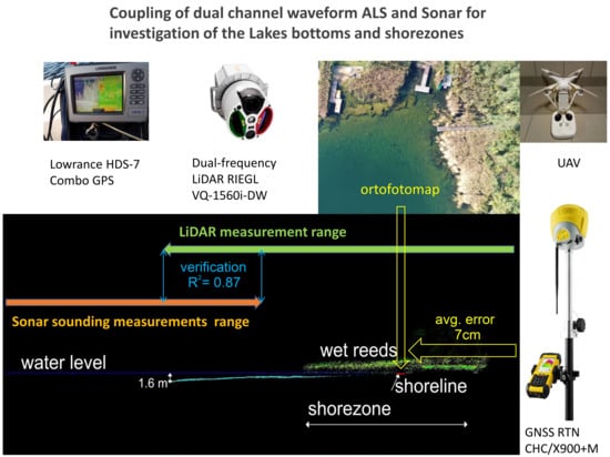
Due to the properties of both devices, the sonar and LiDAR, they have the potential to be used complementarily by fusing both datasets to create a complete image of the lake bottom. Sonar can be used for sub-littoral and pelagic mapping, and LiDAR for littoral mapping. The complete image of the bathymetric model not only combines the data collected by both devices and the information resulting from each of them separately, but also allows them to be compared in the common part, which may be the basis for applying corrections to the datasets. To verify the accuracy of LiDAR for shoreline course determination, combinations of a high-resolution UAV (unmanned aerial vehicle) orthophotomap and GNSS RTN measurements were used. To ensure the homogeneity of the meteorological conditions, the research was carried out on two closely located lakes of different ecological status (difference in water transparency). The main contribution of the paper is testing the ability for application of the dual frequency LiDAR as a complementary tool to the standard echo-sounding method for mapping of the bathymetry of inland lakes. We investigated and described limitations and advantages of both technologies and focused on the comparison of the data captured for the common zone of a lake for both measuring devices. Our investigation allows us to answer the following questions:
Could a Green LiDAR be the complementary part of bathymetry measurements on the shore zone where echo-sounding is impossible to perform due to shallow water depth and aquatic vegetation?
Regarding the findings of Green LiDAR limitations, could it be proposed as a part of the methodology for mapping of the bathymetric relief of inland lakes?
2. Study Area
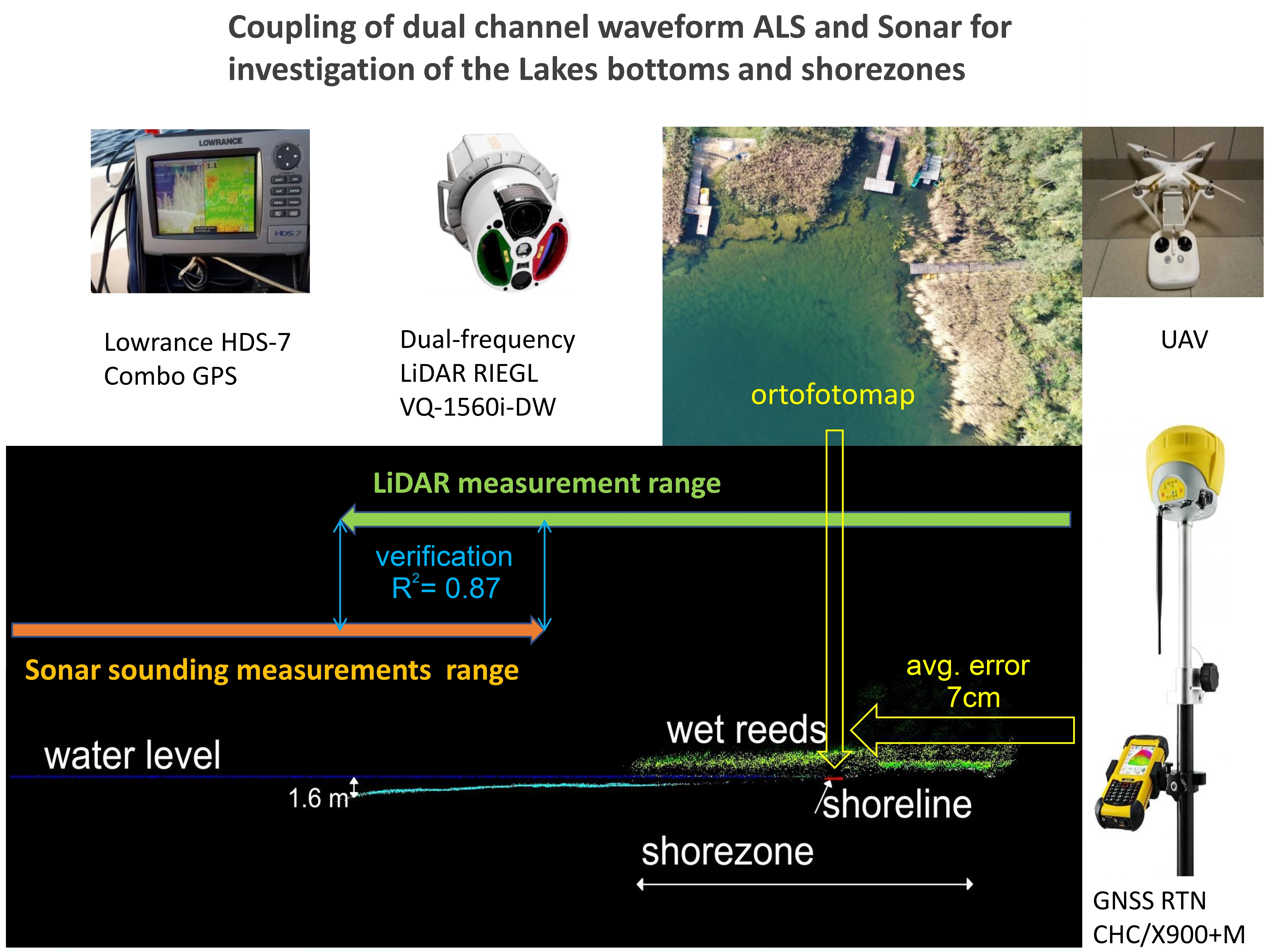
Two ribbon lakes (Białe and Lucieńskie), located in the ice-marginal valley of the Vistula River in central Poland, were selected for the study. They belong to the group of lakes of the Gostynin Lake District, unique in Europe, formed during the North Polish Glaciation and fill deep glacial bowls. The analyzed water bodies stand out against the monotonous landscape (dominant slope inclination within 3–4°). The northern and southern shores of both lakes have significant drops, reaching 30°, while from the west and east, the lakes neighboring with dried peat bogs.
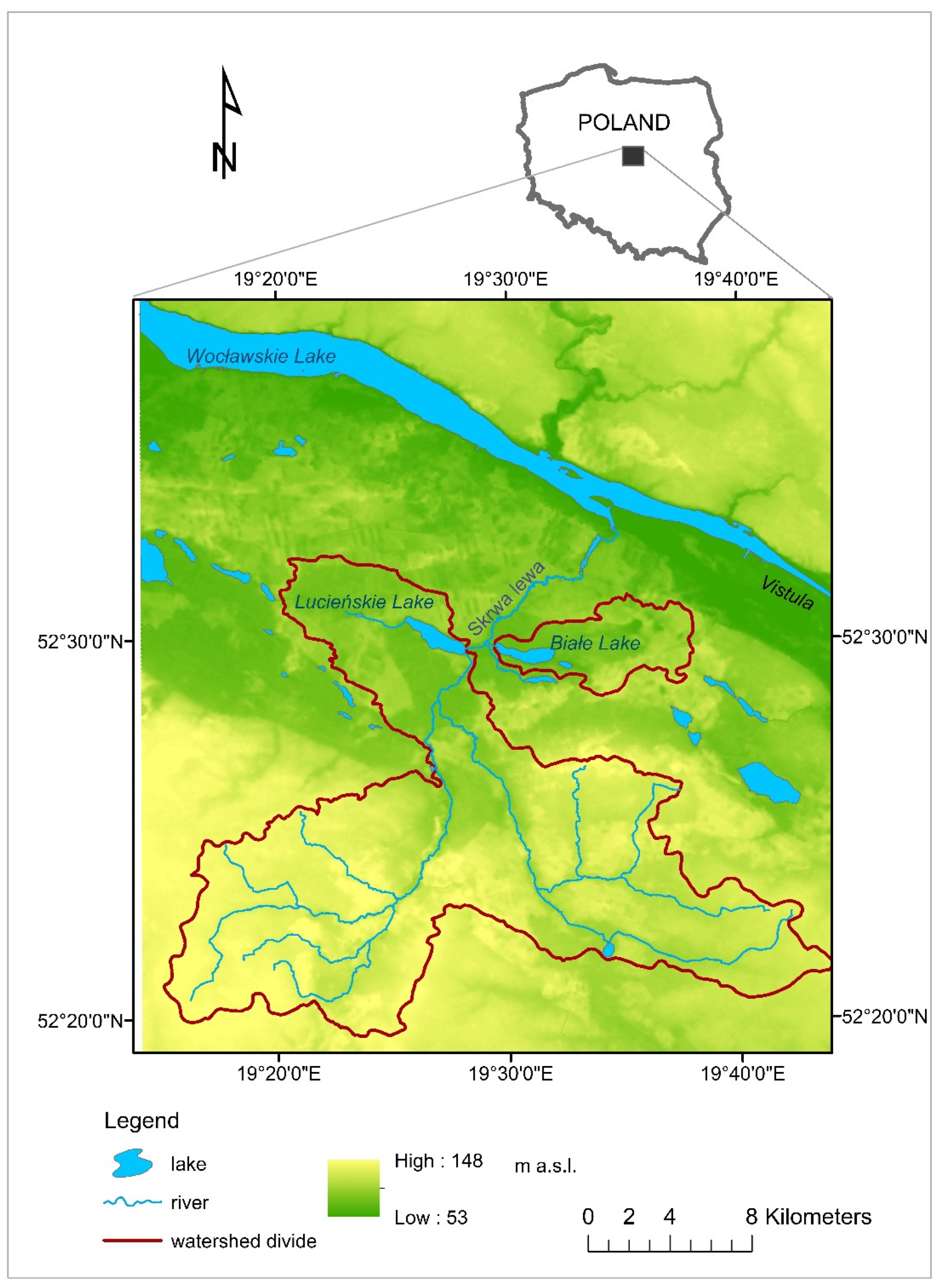
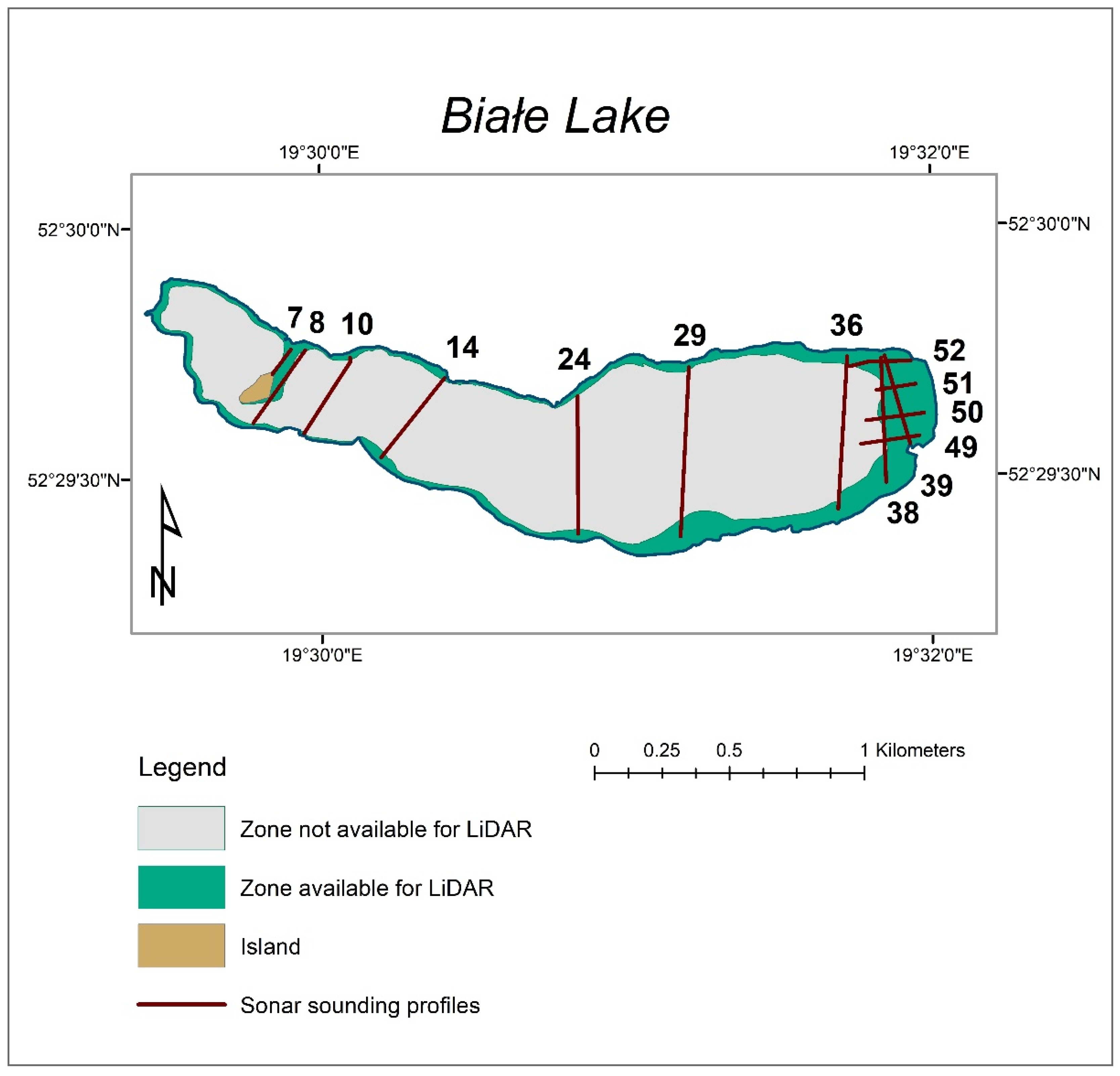
The Białe Lake bathymetry is characterized by a high level of depth changes. It reaches its greatest depths in the central part (31 m), while in the western part, there is a shallow water zone with a small island connecting to the northern shore by a high underwater barrier which separates the shallower overgrown part of the lake. The Lucieńskie Lake has an approximately 20% larger area compared to the Białe Lake and its bottom is more proportional (
Table 1,
Figure 1 and
Figure 2). In the north-eastern and eastern parts of the lake, the slope of the lake basin is the smallest and the coastal zone is the widest. In other parts of the lake, the coastal zone is narrow and the slope of the bottom is larger.
Both lakes, Lucieńskie and Białe, belong to the Skrwa Lewa River catchment, however, they represent different hydrological types. The Białe Lake is supplied by a system of drainage ditches and has a relatively small catchment area of 27 km
2. According to our own investigation performed in the period 2018–2020 by IMGW-PIB, the recorded fluctuations in the lake’s water table reached 35 cm. At the same time, changes in the water level in the Lucieńskie Lake were 10 cm higher. Contrary to the previously described reservoir, the Lucieńskie Lake is a flow-through lake. In the western part, it is supplied by the Skrwa Lewa flowing from the lake just 290 m further north. The catchment area of the Lucieńskie Lake is 309 km
2. The river transports pollutants to the lake from the towns (including the town of Gostynin with a population of ca. 20 thousand and meat processing industries) and agricultural areas located above it. In order to improve the ecological condition of the reservoir, the inflow of the river to the lake was closed in the years 1982–1993. Since 1994, as the water quality of the inflow has improved, the river waters were redirected again to the Lucieńskie Lake. This connection is active during middle and high water levels of the Skrwa Lewa River [
34,
35]. The described hydrological conditions contribute to a better ecological state of the Białe Lake (
Table 2).
According to the assessments of the Chief Inspectorate of Environmental Protection carried out in the period 2016–2019, the Białe Lake achieved a moderate ecological state, while the Lucieńskie Lake achieved a poor state [
37]. This is mainly due to biological elements, especially the development of phytoplankton, which significantly reduces the water transparency. The average visibility of the Secchi disc (SD) is 1.3 m, while on the Białe Lake it is higher and equals to 3.7 m. In the light of measurement carried out in the period 2018–2020, during the vegetation period with intensive development of phytoplankton, the visibility of SD on the Lucieńskie Lake decreased and was below 0.5 m. At the same time, on the Białe Lake it was not less than 3.4 m (unpublished results of investigations performed by IMGW-PIB).
3. Materials and Methods
3.1. Echosouder Measurements and Data
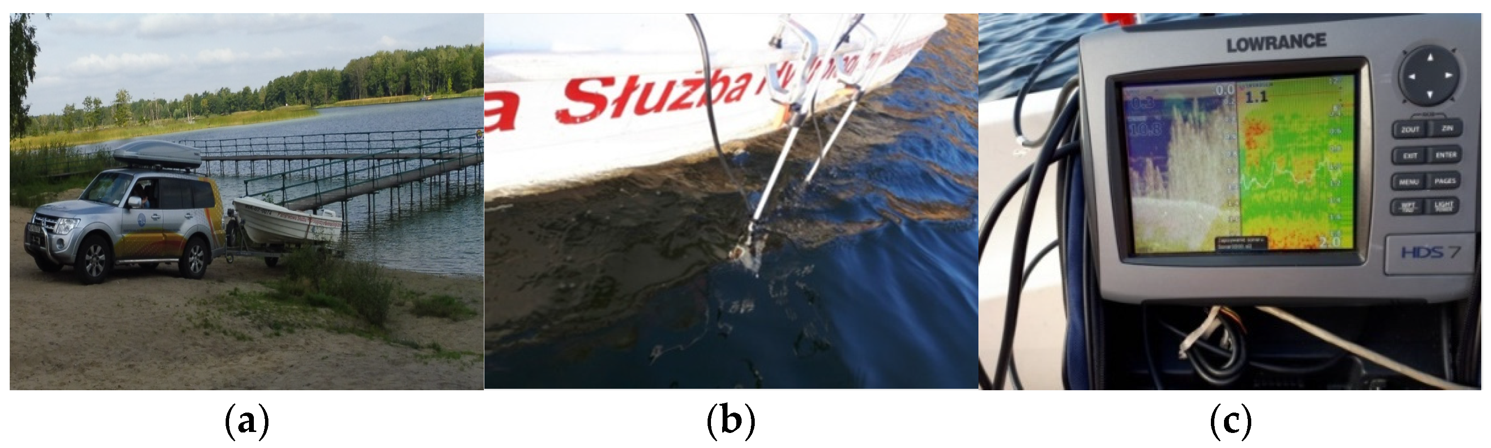
The single-beam Lowrance HDS-7 ComboGPS echosounder with an 83/200 kHz transducer was used for depth measurements (
Figure 3). The minimum depth of the sonar is 0.4 m. The sonar has a 16-channel high sensitivity GPS antenna. This allows to follow the motorboat tracks (more than 10 tracks, 12 thousand points per track). During the measurements, the LSS-1 Structure Scan side sonar was also used to record the shape of the bottom and obstacles disturbing the sonar readings (e.g., bottom vegetation). During the measurements, the route was shown on a color (16-bit) display (6.4″ 163 mm) Full VGA SolarMAX ™ PLUS TFT with a resolution of 480 × 640 (H × W).
Measurements were made from the Texas 360 boat, 3.6 m long, 1.6 m wide, 0.7 m high and 0.60 m draft. The echosounder and side-scan sonar were mounted on outriggers on the port side.
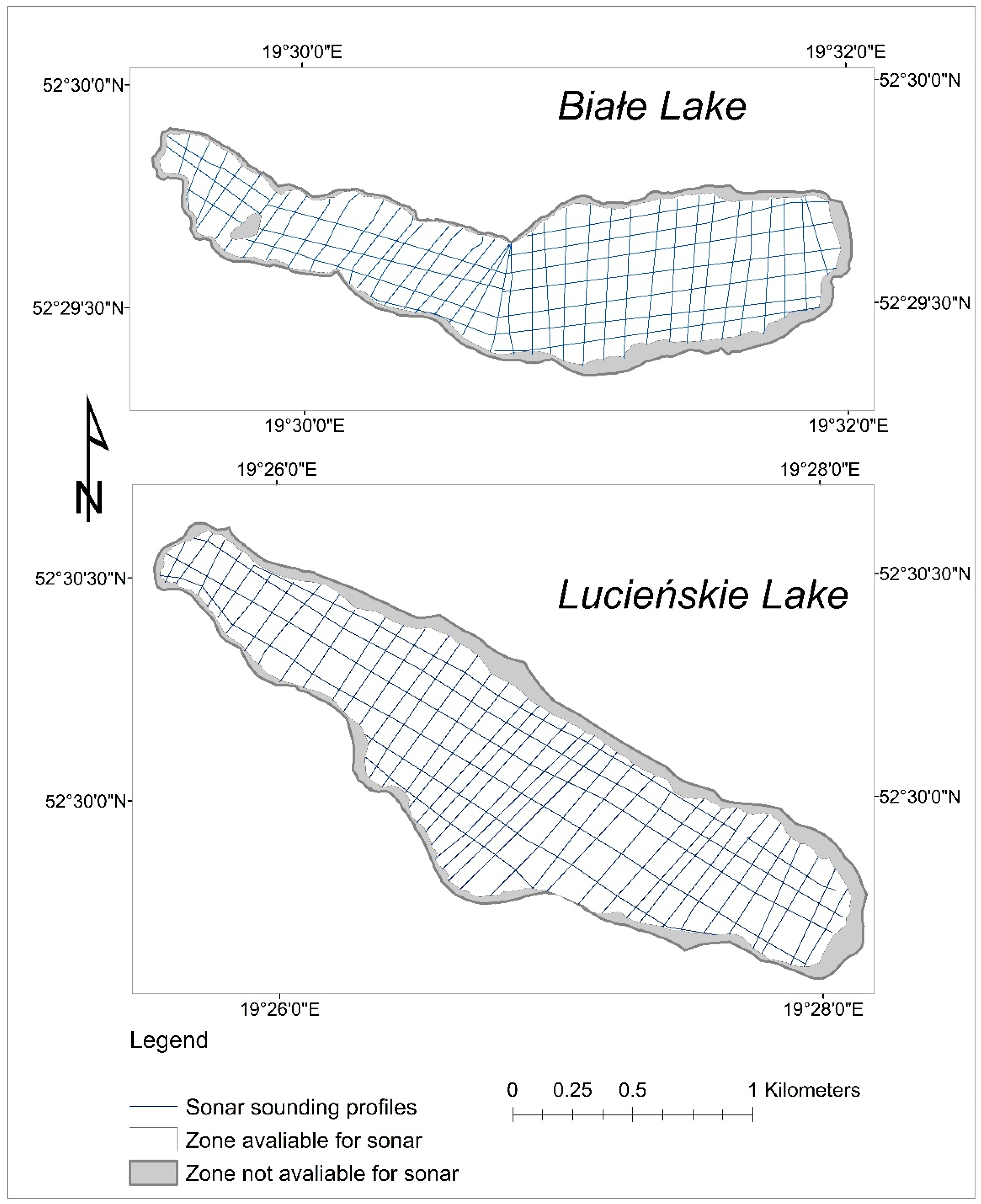
During the measurements, the boat was moving with a speed of approx. 5 m/s. Depth measurements were made in a grid of transverse and longitudinal profiles. The distance between the grid nodes ranged from 50 to 130 m. In total, 52 echograms (39 transverse 13 longitudinal) were created for the Białe Lake. A total of 46 echograms (40 transverse and 6 longitudinal) were created for the Lucieńskie Lake (
Figure 4). Measurements were made as close to the coast as possible. In most cases, it was a distance of 30–40 m from the land line. This distance was increased in the case of the dense and tall aquatic reeds (max. 150 m).
The data obtained from the echosounder (saved in the Sonar Log Files * .SL2 format) were processed by the Sonar Viewer 2.1.2 program to the Comma Delimited Text Files * .csv format, which made it possible to edit the data in the MS Excel and ArcGIS programs. This allowed for an easy selection of information. Information on the location of the measurements as point features (XY in the Mercator reference system) and the depth (in m) measured at the sonar frequency of 200 kHz (dedicated to small depths) were left for further analysis. In the next step, the coordinate system was converted to the EPSG system: 2180 (Poland CS92). Due to the high frequency of depth measurements and the change in the speed of the boat with a dense cover of bottom vegetation, the sonar performed from several to a hundred soundings for a specific combination of coordinates. To avoid information noise, duplicate information was removed for each pair of coordinates and three values were determined for each pair of coordinates: minimum, mean and maximum depth values. The mean value was used for comparison with the results of the LiDAR.
3.2. LiDAR Technology and Data Analysis
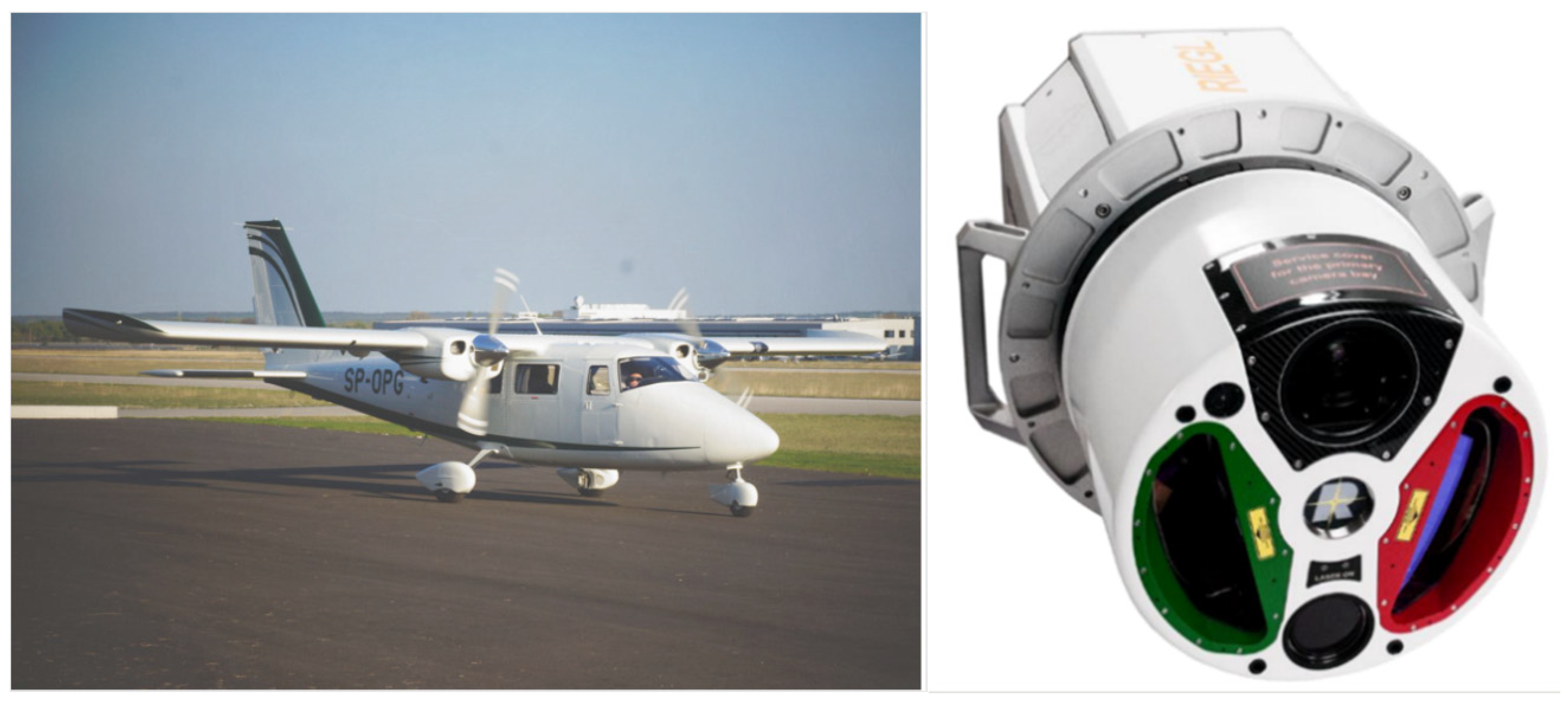
LiDAR data were obtained on 5 September 2019 during a single photogrammetric mission. The measurements were made using the SP-OPG platform by Opegieka Sp. z o.o. (Vulcanair P68C plane,
Figure 5). It was equipped with a VQ-1560i DW laser scanner which allows for the measurement in two channels: green and infrared. It performed scanning at different angles. The basic parameters of the LiDAR data registration mission include:
Flight altitude: 1400 m;
Field of View (FOV): 58 degrees;
Laser pulse repetition frequency (PRF): 1 Mhz (for both channels);
Designed point density: 5 points/m2 (for both channels);
LiDAR channel 1 spectral length @ 532 nm;
LiDAR channel 2 spectral length @ 1064 nm.
As a result of the designed flight, a point cloud with a density of 10 points per m2 was obtained, which covered 97% of the Lucieńskie Lake (including the buffer zone) and 90% of the Białe Lake (including the buffer zone). Data postprocessing was performed with the use of three software packages: RiPROCESS (Riegl) (alignment, georeferencing), RiHYDO (Riegl) (refraction correction) and TerraScan–TerraSolid (data classification).
The initial step of the LiDAR data analysis was to consider the effect of refraction on the measurements of lakes’ bottom depth. For this purpose, the RiPROCES software was used for classification of the points defining the water surface from which the WSM model (Water Surface Model) was created. On the basis of the created model, the influence of refraction was taken into account and calculated in the RiHYDRO software. After exporting data from RiPROCESS to LAS format, a point cloud was automatically classified in TerraScan into the following classes:
Class 1—Default—points not classified;
Class 2—Ground—points defining the terrain surfaces;
Class 3—LowVeg—points defining low vegetation (0 m–0.4 m);
Class 4—MidVeg—points defining medium vegetation (0.41 m–2.0 m);
Class 5—HighVeg—points defining tall vegetation (>2.01 m);
Class 6—Building—points defining the roofs and walls of buildings;
Class 7—Noise—noise;
Class 9—Water—points that define the water surface;
Class 13—UnderWater—points that define the bottom of the lake after taking into account the effect of refraction.
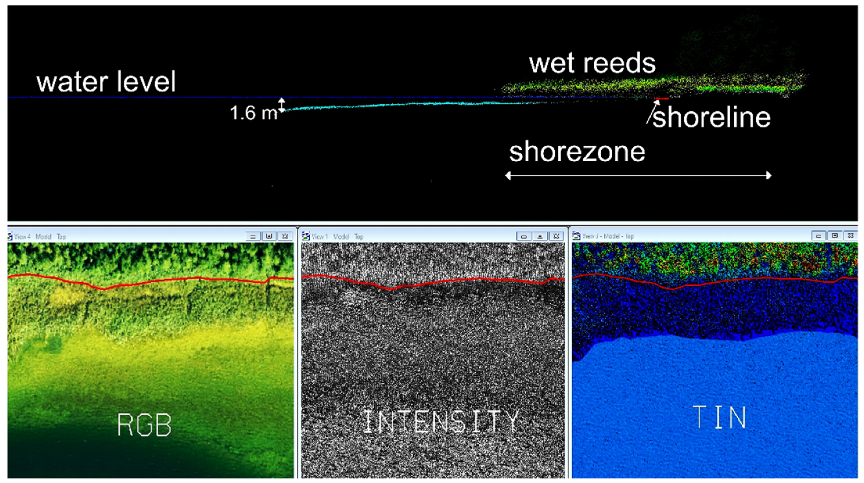
After the automatic data classification was performed, the range of the surface water boundary (shoreline) was manually digitized to obtain the shoreline of both lakes. For this purpose, the previously classified LiDAR data were used as a visual aid, displaying them in the “intensity”, “RGB” and “DTM” views. Using the range of the lakes prepared in this manner, the final classification of points defining the lakes surface (Class 9—Water) and the bottom of the lake (Class 13—UnderWater) (
Figure 6).
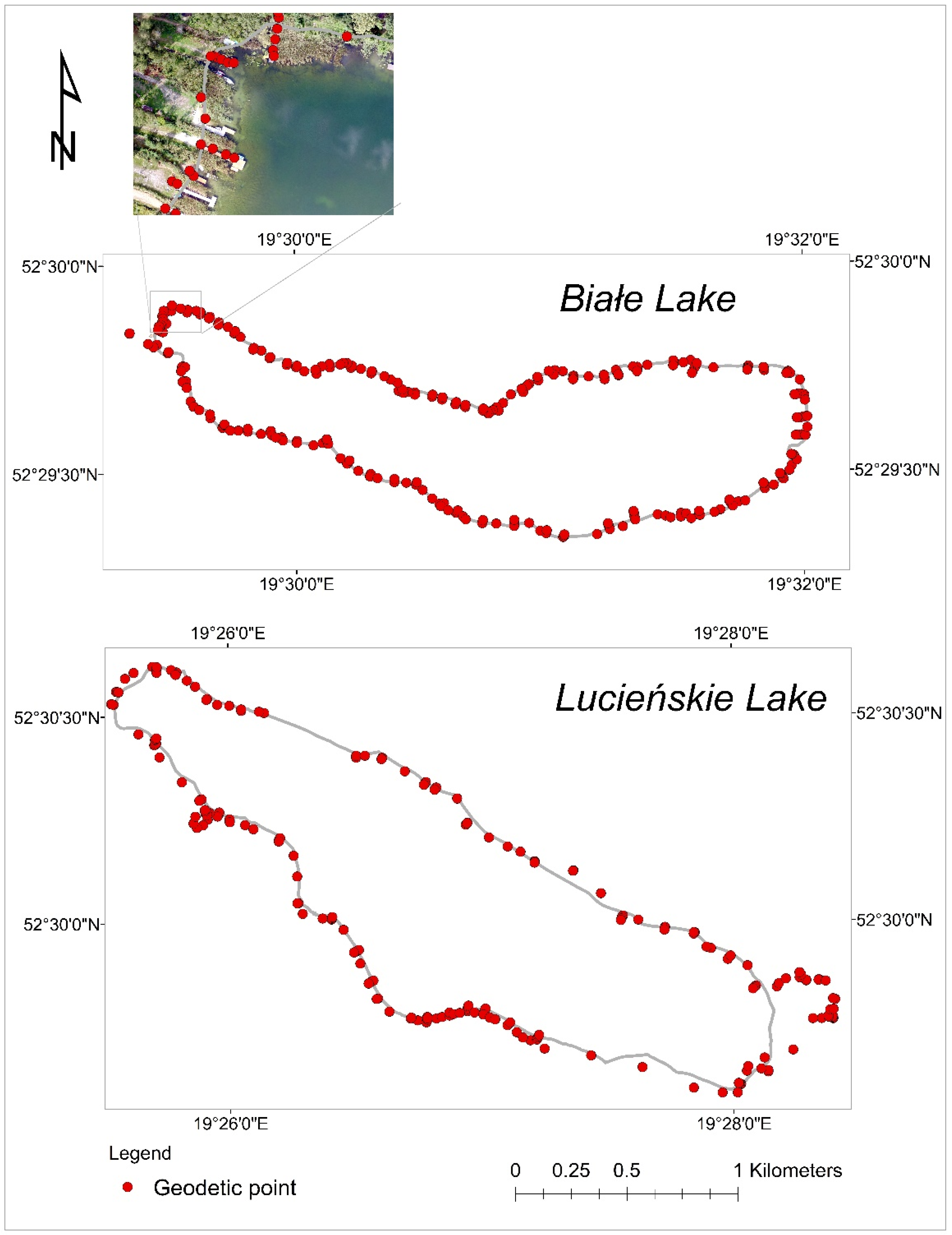
3.3. Shoreline Geodetic Surveying
In order to identify the shoreline of the lakes, geodetic measurements of the water table range and additional points, located in cross-sections perpendicular to the course of the shoreline covering the land–water transition zone of both lakes, were performed. For this purpose, the GNSS CHC/X900 + M with RTN mode (Real-Time Networks) receiver was used, based on surface corrections from the network of reference stations of the ASG-EUPOS system (
www.asgeupos.pl, accessed on 1 April 2021) with an accuracy of +/−0.05 m. The closed areas around the Lucieńskie Lake and inaccessible wetlands located between the lakes were omitted. Measurement points were selected in accessible areas of the shoreline (
Figure 7) using beaches and exposed (not covered by forest) shores, platforms, and other water structures. A total of 261 points measured on the Lucieńskie Lake and 413 points on the Białe Lake, were located in cross-sections perpendicular to the shoreline and placed where the vegetation did not limit the visibility. The obtained results were transformed to .shp format (ArcGIS) in the Coordinate System 1992 (EPSG code: 2180) and in the Kronsztadt 86 height system.
The obtained results were compared with the shoreline course determined on the basis of the LiDAR analysis. On the day of the geodetic measurements, the water table elevation was 72.53 m above the sea level, and on the day of the LiDAR raid, it was 72.54 m above the sea level. Taking into consideration that this is a small difference, for the purposes of further analyses, it was assumed that the range of the water table determined by field measurements and laser data is the same.
3.4. UAV Data Capturing and Producing Ortophotomaps
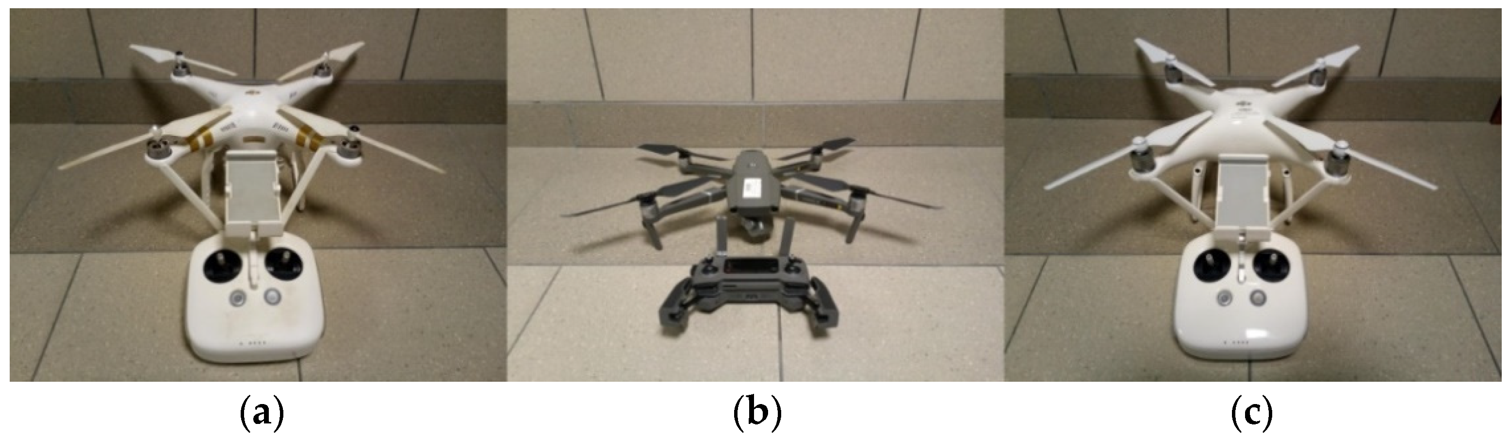
The main purpose of using an UAV was to collect ground truth information to analyze the LiDAR technique for determining the water body extent. The source data for the preparation of a set of orthophotomaps in the form of geocoded RGB photos were obtained using the DJI Mavic 2 PRO unmanned system (DJI, Shenzhen, China) and the DJI Phantom 3 Pro and Phantom 4 Advance (DJI, Shenzhen, China) (
Figure 8). The flights were carried out in autonomous mode along the paths previously determined by the Pix4D Capture software (Pix4D S.A., Prilly, Switzerland). The area of the UAV mission covered the shore zone of the lakes (together with the buffer zone). The flying height was chosen based on the size of the Ground Sample Distance (GSD) at the level of 3 cm. The flight paths were planned so that the mutual coverage of photos from neighboring paths was not less than 75%. The UAV aerial photographs were collected during the LiDAR acquisition mission and three weeks later.
The Ground Control Points (GCP) were selected in the form of “natural” points and by using black and white artificial discs of 0.3 × 0.3 m, these points were then measured using the Topcon GRS-1 GNSS system (corrections from the ASG-EUPOS—
www.asgeupos.pl, accessed on 1 April 2021) with RTN (Real-Time Networks) mode, with an accuracy of +/−0.05 m. The Metashape Photogrammetric software (Agisoft LLC, St. Petersburg, Russia) was used to generate an ortophotomosaic of the lakes using the SfM (Structure from Motion) algorithm and GCP coordinates. Moreover, photos in which water constituted more than 95% of the photography area and after visual assessment of the point cloud, points with locations significantly differing from the rest of the model (or photos to which they belong) were rejected.
Finally, after unsupervised classification and manual corrections, points classified as ground were used to generate the DTM creating mosaic. The final ortophotomap was exported in the Coordinate System 1992 (EPSG code: 2180) and then, in the case of sections with no GCP, a geometric correction in the QGIS software (OSGeo, Beaverton, OR, USA) was performed.
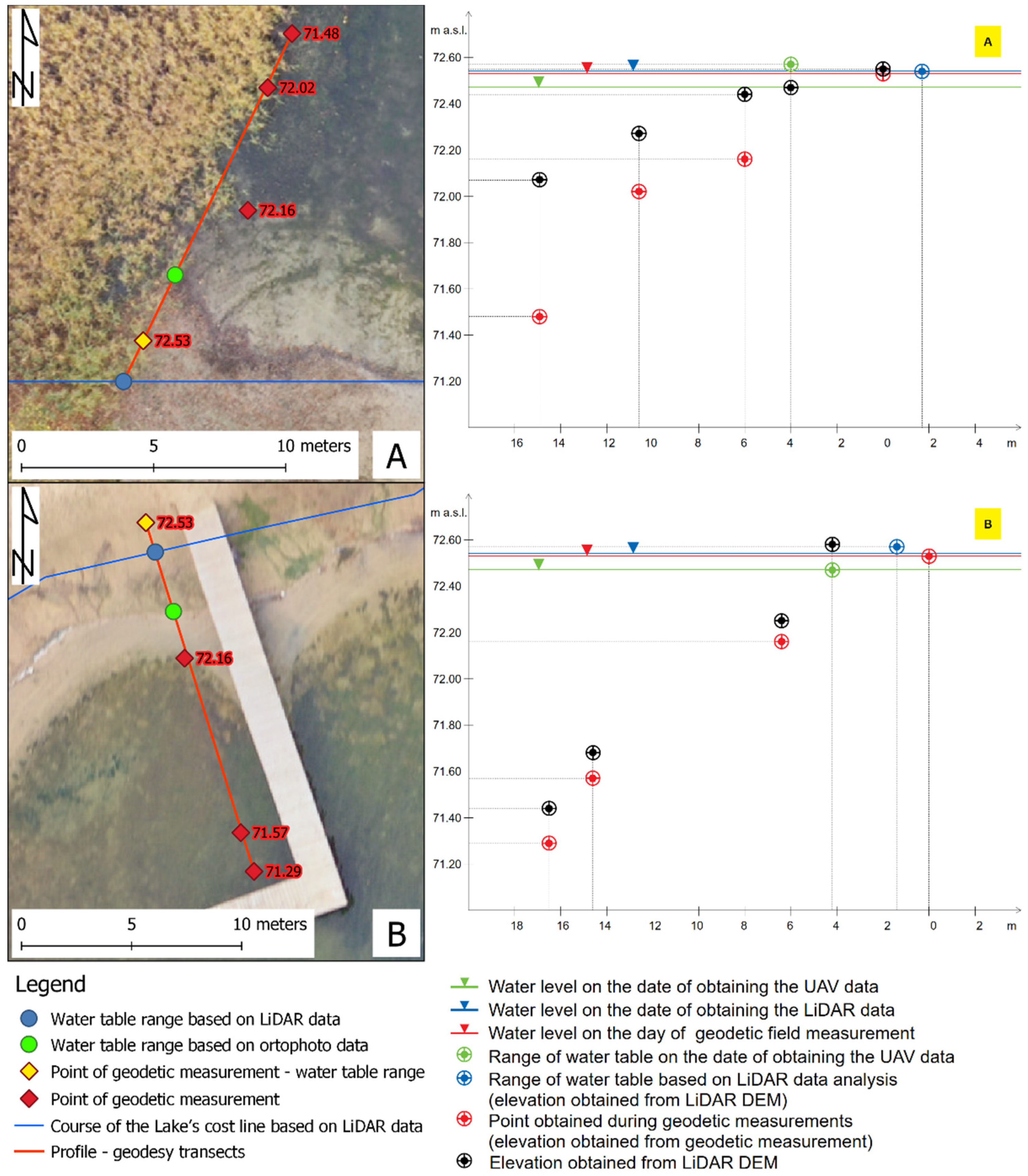
3.5. Identification of the Shoreline in Measurement Cross-Sections
In the next step, the visual analysis of point coordinates in cross-sections and point height was performed to clearly indicate the water–shore border point. In order to interpret the course of the shoreline, orthophotos taken from UAV photos obtained on 12 October 2019 were analyzed in addition to the elevation model. The digital elevation model (DEM) was developed on the basis of classified LiDAR data (“Ground” and “underwater” class) with the LAS2DEM tool included in the LAStools package (Rapidlasso GmbH, Gilching,Germany). The shoreline obtained from LiDAR data analysis was verified by comparing it with the UAV orthophotomap.
As a result of the visual analysis, a shoreline was identified, as well as the height of the water table was compared with DEM in the cross-sections.
Moreover, the range of the water table was determined on the basis of the digitized line of the lake shore (see
Section 3.6) and the distances between the measured and determined profile points were calculated.
3.6. Lake’s Water Level Changes during Investigation of the Shoreline
In order to assess the relationship between the results of different measurement types (geodesy, UAV data, sonar and LiDAR) which are collected at different times, the analysis of the water table level at a particular date is of highest importance. Taking into account the fact that the level of the lake’s water table differed during the measurements performed with various methods (
Table 3), the analysis of the shoreline course and water depth were reduced to the water table level occurring during sonar measurements. The water table level was measured in the transects perpendicular to the lake coastline. The results of these measurements allowed for the analysis of differences in the water level occurring on the days of LiDAR scanning and sonar scanning (see
Section 3.5).
3.7. Statistical Analysis of Sonar and Lidar
In the next stage, the dependence and stationarity of the sequence obtained from both measuring devices were verified. In the first case, the runs test [
39] was used, verifying the number of observations above and below the median value and determining the test probability, i.e., the
p-value. Moreover, the autocorrelation of sonar Z (the lake’s water depth measured by the SONAR, in meters) and LiDAR Z (the lake’s water depth measured by the LiDAR, in meters), which represent a measuring sequence of the sonar and LiDAR data, respectively, for the delay Lag = 100, was investigated. The Lag assumed in the study was considered sufficient to identify the occurrence in data sequences. The stationarity of both analyzed measurement sequences was verified with the use of two tests, i.e., the Augmented Dickey–Fuller test and the ADF test [
40], for which the null hypothesis assumes non-stationarity of the tested sequences, and the Kwiatkowski–Phillips–Schmidt–Shin (KPSS) test [
41], in which the null hypothesis assumes the stationarity of the random variable under study. The ADF test takes into account the existence of a trend in the tested measurement sequences by appropriate selection of the critical value of the test for the significance level of α = 0.05 [
40].
4. Results
4.1. Verification of the LiDAR Method in Determining the Extent of the Shoreline and the Water Table Level
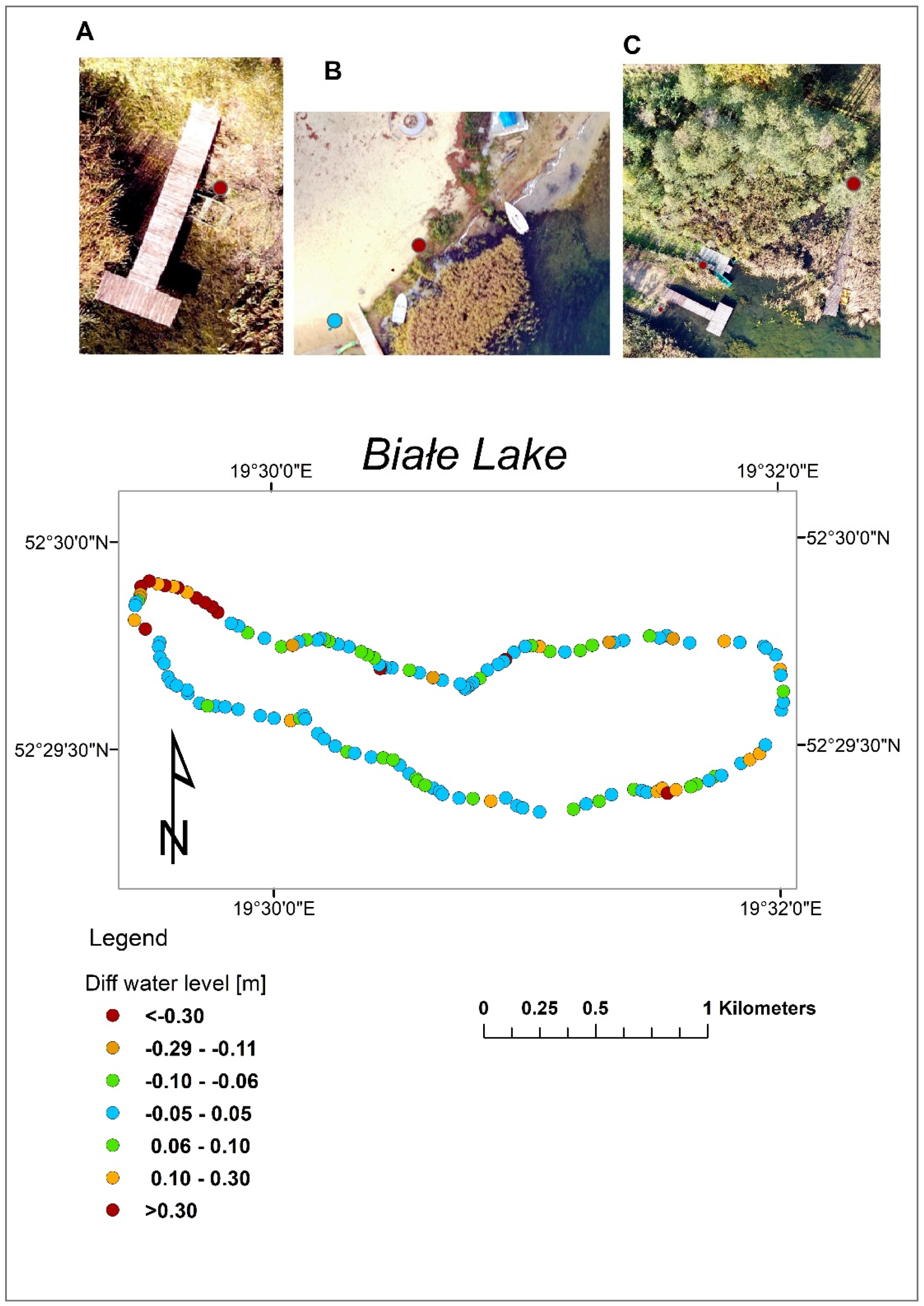
The Białe Lake water table level was verified by comparing values taken from the DEM generated from green beam LiDAR data that covered the lake bottom in the shallow coastal zone with geodetic points measured in the coastal zones marking the extent of the water table. At the outset, points that DEM did not cover and points on geodetic transects, descending below the water table, were eliminated. Subsequently, the extracted points were visually inspected point-by-point using the UAV ortophotomaps (
Figure 9). As a consequence, the verification of the position of the water table was analyzed for 145 points. The spatial differentiation of the water table verification results is shown in
Figure 10. The greatest discrepancies in water table level measurements by the two methods occur in the north-eastern coastal zone where there are numerous piers in the narrow stripes of the cut reeds. Coastline interpretation based on LiDAR data is often showing in these places the course of the pier and not the actual coastline. Another reason for the differences may be due to the watercraft moored next to the piers, which can change their position during scanning in relation to the geodetic measurement, which results in measurement heterogeneity (
Figure 10A,B). Another problem is the transformation of coastal zones due to the anthropopressure. One example is dumping the sand on the beach (
Figure 9B), which, with a one-year difference between the geodetic measurement and LiDAR scanning, may be the cause of inaccuracy. Another identified problem that may have an impact on the height differences is the presence of dense tree crowns covering the water–land boundary line (coastline) (
Figure 10C) and the proximity of reed beds (
Figure 9A).
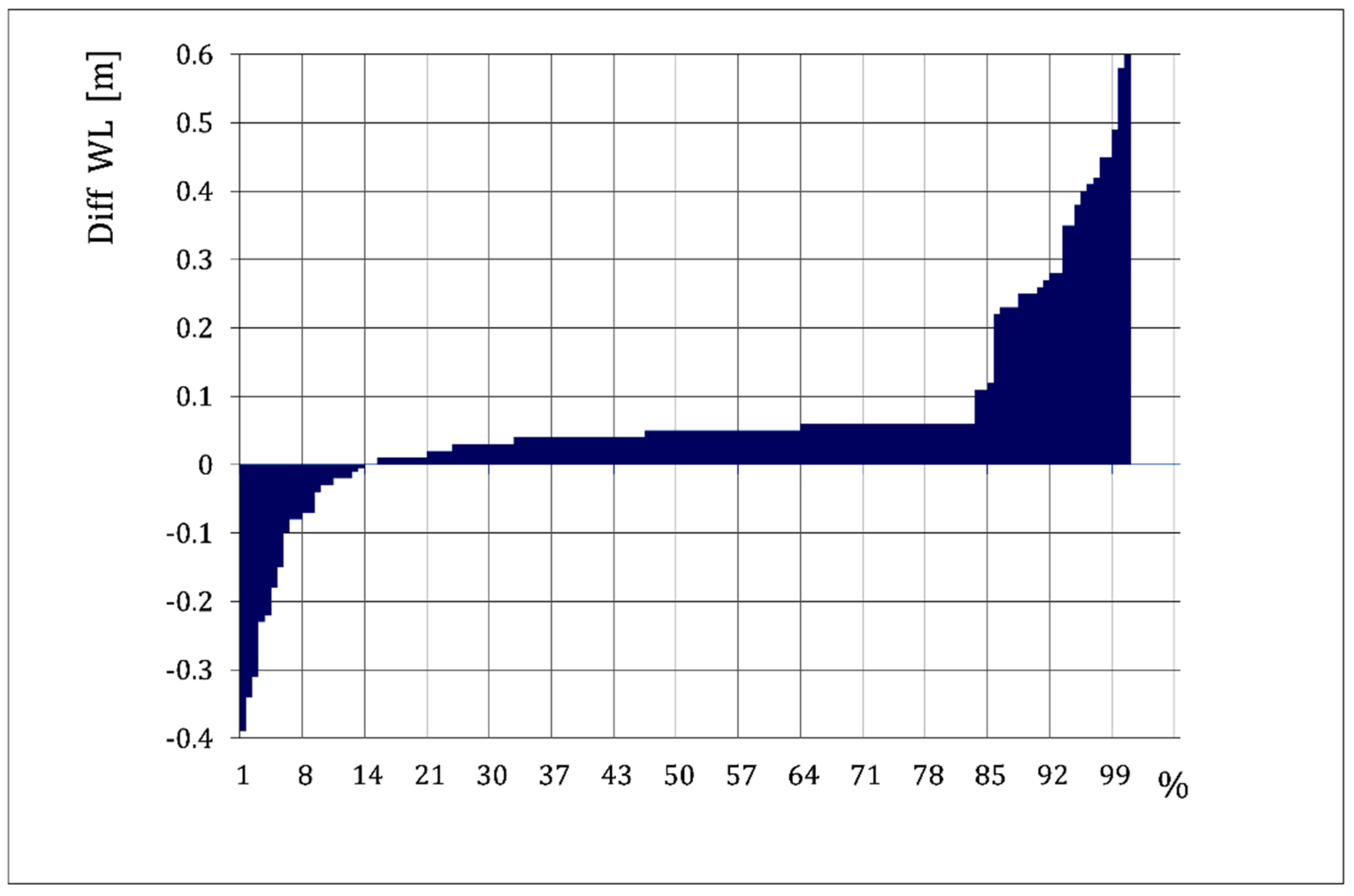
The percentage distribution of the differences of the water table level readings determined by the compared methods is shown in
Figure 11.
In 78% of the cases the error was negligibly small and it did not exceed 6 cm. In addition, 8% of the values are underestimated, including 2% of which exceed 30 cm. A much larger percentage corresponds to values that are overestimated and as much as 7% exceed 30 cm, which is the range of water table level fluctuations. The mean error in determining the elevation of the land based on LiDAR, assuming geodetic measurement as a reference, is 7 cm (the absolute mean value of the difference in water table measurements by LiDAR and geodesy). The standard deviation of differences is equal to 16 cm.
The Lucieńskie Lake was not included in the above analysis due to the properties of the reservoir that prevented penetration of the water column by the laser beam, and thus the DEM model was not created on the basis of bathymetric data from the classified LiDAR point cloud.
4.2. Comparison of LiDAR and Sonar Bathymetric Measurements
LiDAR measurements were made at low water level: Białe Lake–72.54 m above sea level, Lucieńskie Lake–72.89 m above sea level. Under these conditions, the length of the shoreline was 7.74 km and 10.13 km (including the island), respectively. As a result of LiDAR scanning, a total of 70,829,903 measurement points were obtained. The results of their classification are presented in
Table 4. When analyzing the classification results, it should be noted that the effectiveness of the conducted research of the lake bottom measurements differs in both lakes (
Figure 12,
Table 5).
The capability of scanning the bottom of the lake with sonar was greater in the case of the Lucieńskie Lake, where the bottom relief is less diversified. On the other hand, the LiDAR “Underwater” Class encountered limitations. In the case of Lucieńskie Lake, the green LiDAR beam did not penetrate the non-transparent water column (visibility of the Secchi disc 0.5 m). In the case of Białe Lake, where the visibility of the Secchi disc was 4 m, it reached a depth of 1.6 m, which made it possible to measure the depth on 20% of the lake’s surface, usually in the coastal zone (
Figure 12).
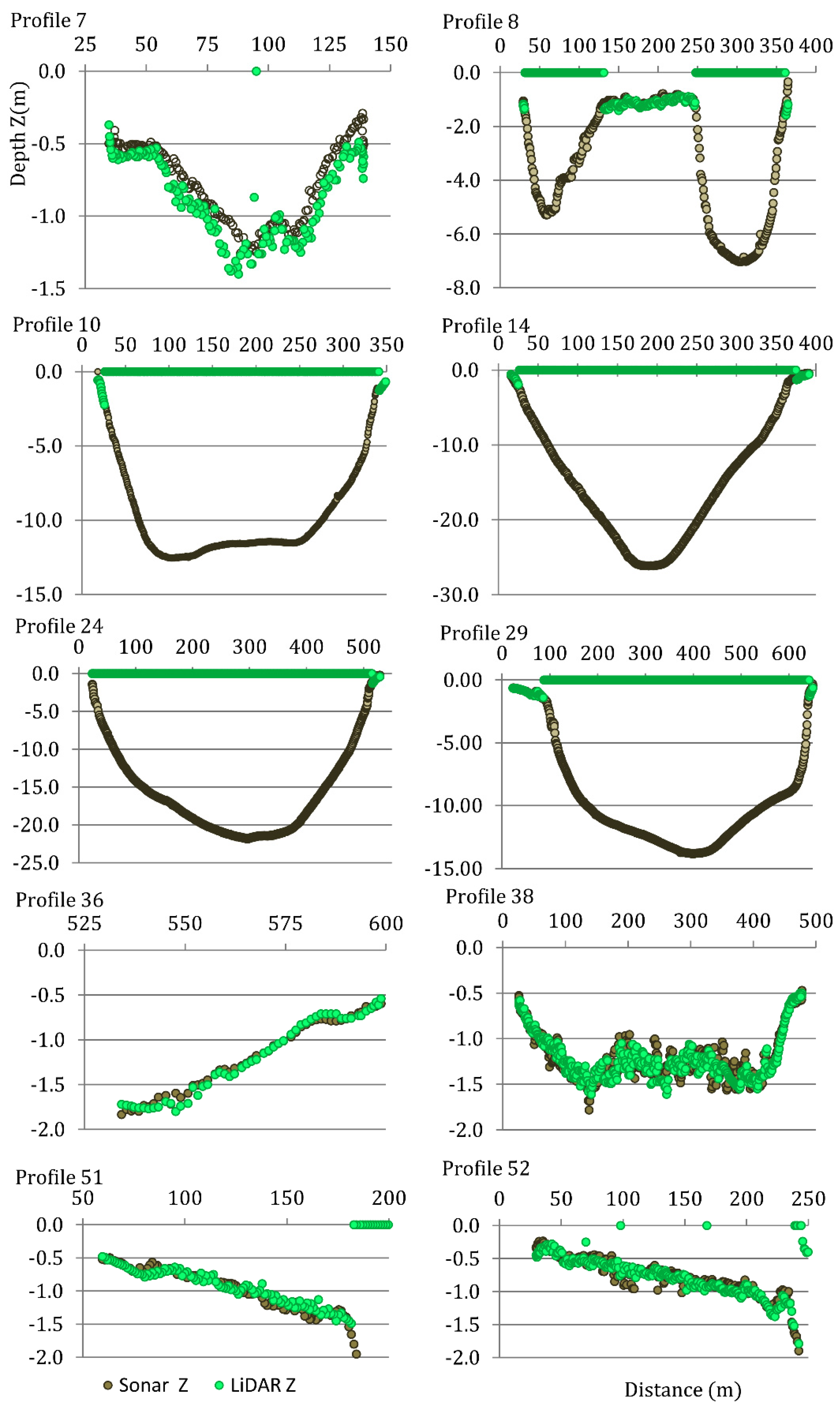
Figure 13 presents selected transects of the lake water body obtained with the use of the two compared methods. The combined measurements of both methods covered the zone defined by the depths from 0.5 to 1.6 m and these were used for comparative statistical analyses. A total of 1359 pairs of points were selected.
After confirming the dependence and stationarity of the tested measurement sequences (
Table 6,
Figure 14 and
Figure 15), the correlation between the results of the measurements of the depth Z was examined.
Two standard statistical methods have been used for correlation analysis, namely, (1) the non-parametric Spearman–Kendall rank correlation test and (2) the parametric Pearson’s linear correlation coefficient test (
Table 7). Negative and positive values indicate a downward or upward trend, respectively. The coefficients also allow to determine the strength of the current trend. The closer the values are to −1 or +1, the stronger the relationship between the studied random variables. The Pearson’s coefficient determines the proportionality (i.e., linear dependence) of the variables to each other, while the Spearman and Kendall coefficient determines any monotonic relationship, also non-linear. In the case of dependent random variables, the procedure of calculating the Pearson coefficient takes into account the calculation of variance that includes covariance [
42]. The non-parametric Mann–Kendal test [
43] was used to detect and test the significance of the trends in changes in the measurement sequences.
Then, a linear regression model of Sonar_Y = f(LiDAR_X) was presented (
Table 8), where the dependent variable is the Sonar_Y measurements and the independent laser measurements. The regression coefficients (β), standard error of β estimation (standard error β), coefficients of lower and upper bound of intercept and independent variable, LiDAR_X, t-test testing the significance of each regression coefficient expressed as the quotient β, standard error β, Pearson’s correlation coefficient (r), coefficient of determination (r
2), and standard error of estimation were computed. Moreover, using the global F test (Fisher–Snedecor), three equivalent null hypotheses were tested: H0: β1 = 0—significance of the slope coefficient, H0: r
2 = 0—significance of the determination coefficient and H0: β1x + β0 = y—significance of the linear relationship between the analyzed variables, where β1 is the slope, β0 is the free term and x and y, respectively, are the independent and dependent variable. The null hypothesis that the independent variable x (LiDAR) had no effect on the investigated dependent variable y (in Sonar_Y) was verified. The significance level of the model was
p < 0.005.
Three statistical measures were used to assess the model quality (
Table 9): mean absolute error, MAE (mean absolute error), root mean square error, RMSE, Nash and Sutcliff efficiency coefficient, NSE (Nash–Sutcliffe efficiency).
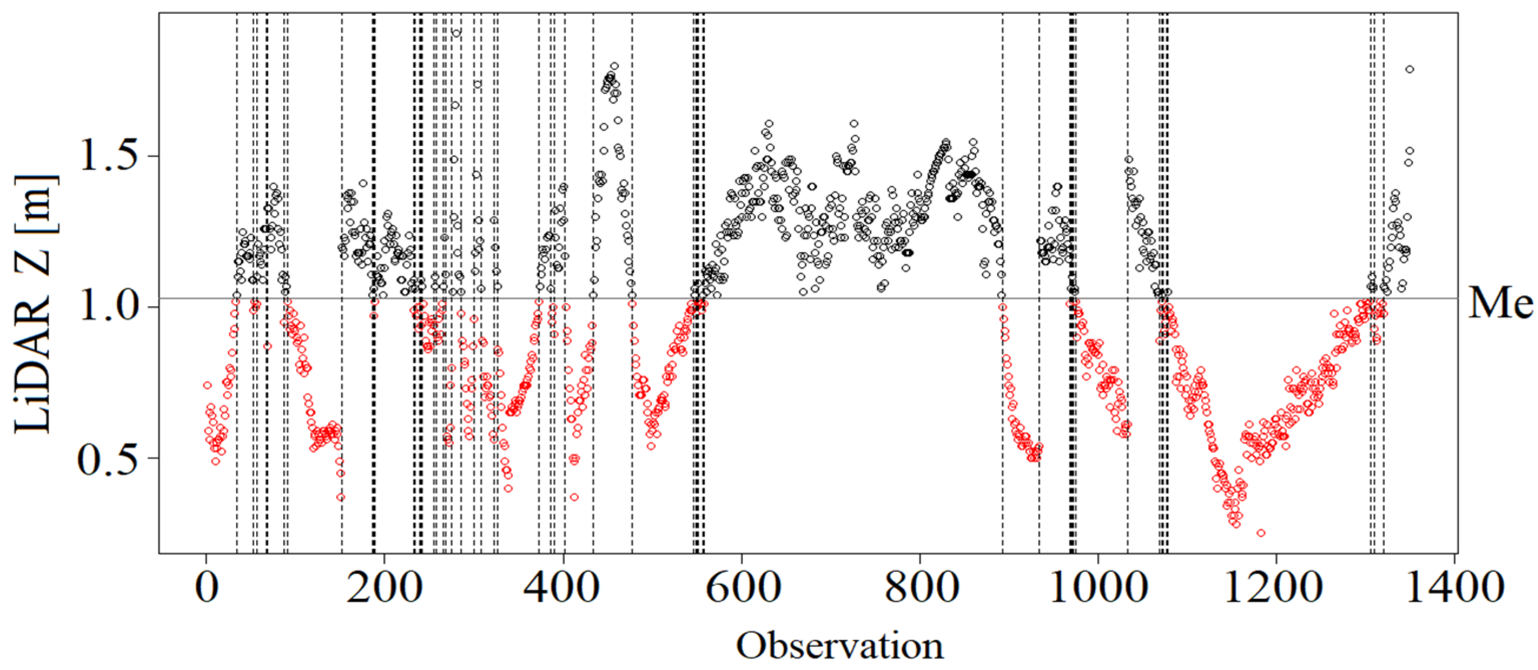
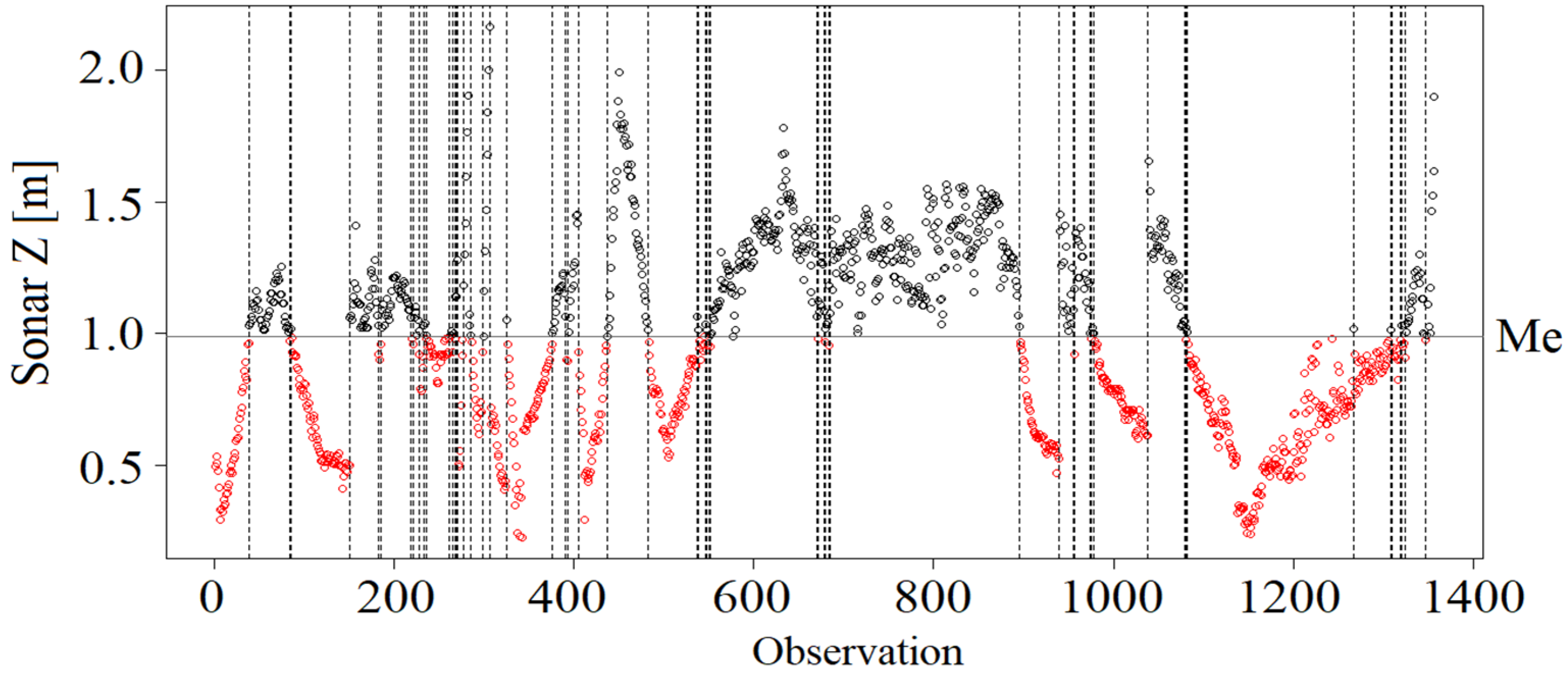
Statistical tests of the two analyzed variables Sonar Z and LiDAR Z sequences confirmed their dependence and stationarity. The runs test showed that for each analyzed variable, the number of observations above and below the median was different (
Figure 14), and the
p-value was lower than the significance level of α = 0.05 adopted in the study (
Table 6). In such a situation, it was concluded that the verified null hypothesis about the independence of the tested random variable should be rejected. It was found that the realizations of both sequences are not random, and their selection for the sample is subject to a tendency or cyclicality, i.e., the tested random variables are dependent.
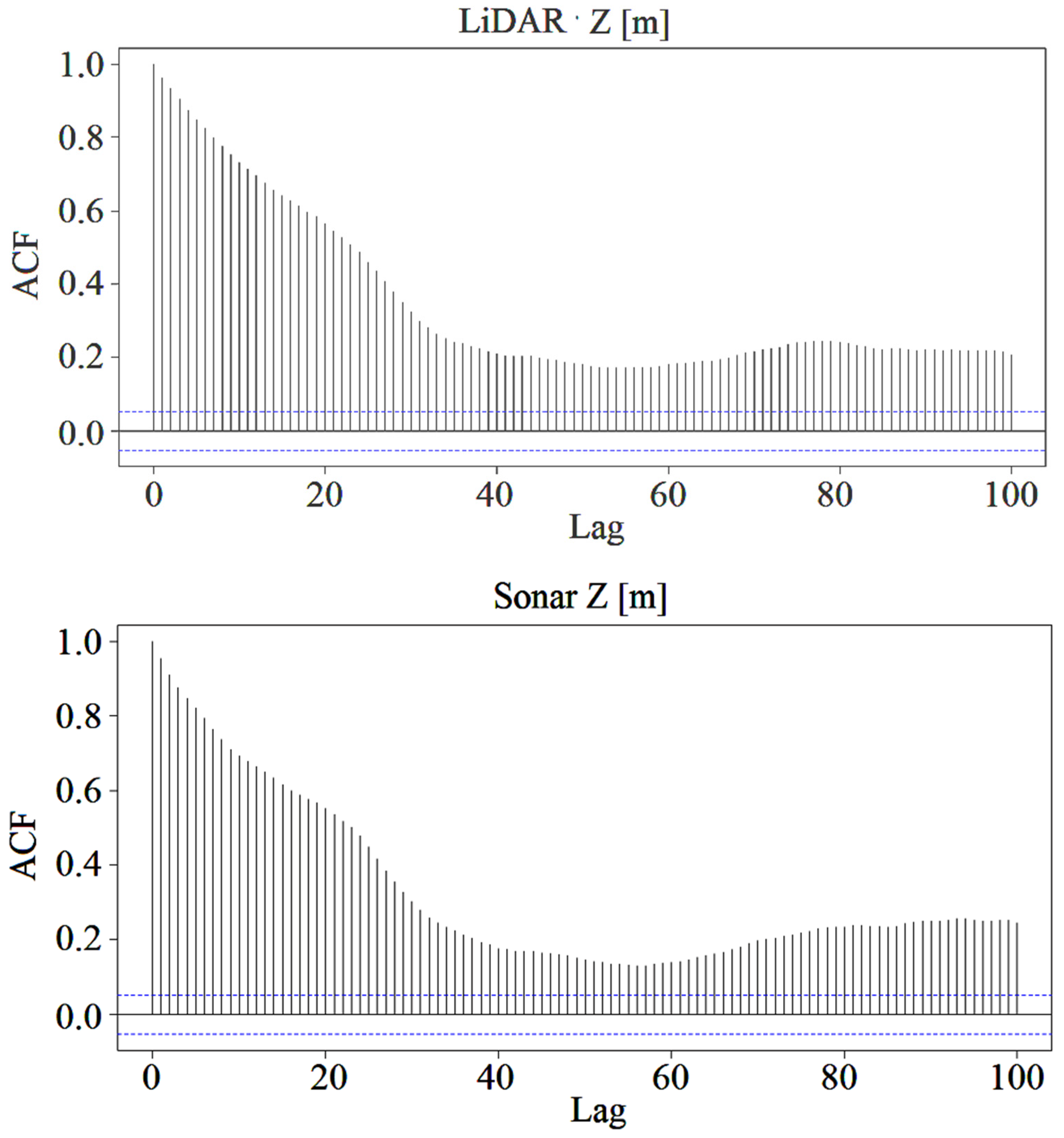
The autocorrelation studies of both measurement sequences are shown in
Figure 15. No periodic fluctuations were detected in the charts.
The stationarity verification by the ADF test indicated that the test statistic is lower than the critical value at the significance level, α = 0.05 (
Table 6). Therefore, H0 concerning the presence of the unit root in both tested sequences should be rejected in favor of the alternative hypothesis about the stationarity of the tested random variables. A similar result of stationarity assessment was obtained using the KPSS test [
41]. In both cases, the test statistic was higher than the critical value adopted in the study, thus there was no reason to reject H0 about the stationarity of the studied random variables (
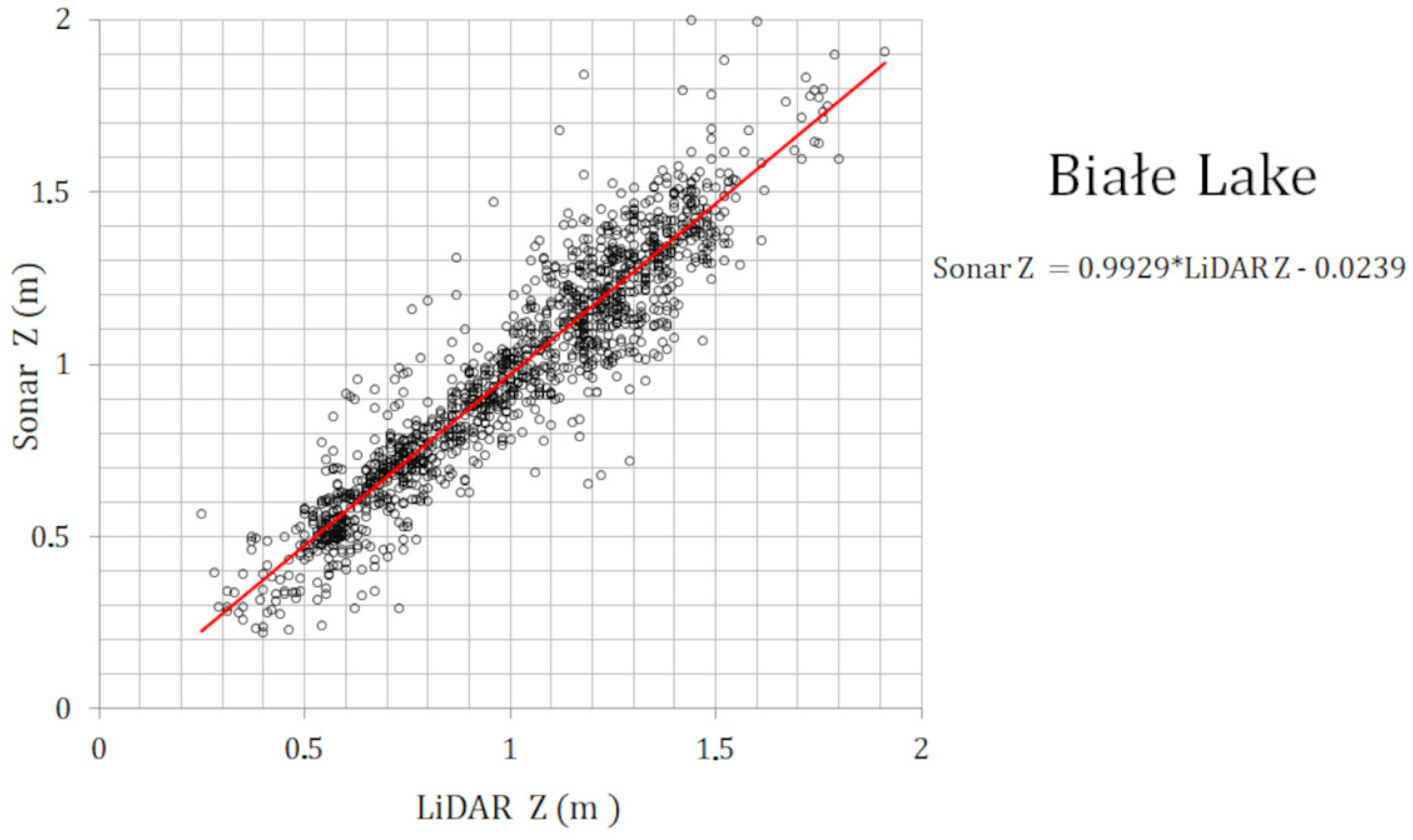
Table 6). Subsequently, the studies carried out in the coastal zones of the Białe Lake confirmed a statistically significant linear relationship between the measurements obtained from sonar and from LiDAR (
Table 9). A linear model was used to analyze the relationship Sonar_Y = f (LiDAR_X) (
Figure 16). The ADF test included in the calculations resulted in a statistically significant tendency in the LiDAR data using the Mann–Kendall test (
Table 7) by appropriate selection of the critical value of the test at the significance level, α = 0.05 (
Table 6).
The results of the regression analysis confirmed the existence of a significant linear influence of the LiDAR-X random variable on the tested Sonar-Y dependent variable, with
p < 0.05 (values in bold). The Fisher F-test has a value significantly higher than the test
p-value. This means that the null hypothesis is rejected and the evaluation of the regression coefficients is significant (
Table 8).
The results of the quality assessment of the Sonar_Y = f(LiDAR_X) model according to statistical measures are presented in
Table 9. High quality measures of the used model were obtained.
5. Discussion
The assessment of the water table range in the shore zone of natural lakes is a technically difficult task due to the dense reed vegetation in the shore zone. The dense reed zones restrict surveying from the boat, while the presence of wetlands limits the availability of shore for geodetic measurements performed from land [
44,
45]. Additionally, trees and shrubs growing in the shore zone prevent airborne passive imaging (even from low distance) and precise assessment of the shoreline [
46,
47]. Apart from that, the shore zone under the influence of anthropopressure is remodeled, causing changes in the shape of the shores in a relatively short time (e.g., construction of piers, building artificial beaches, reed mowing). In the interpretation of aerial imaging, problems may be caused by, e.g., watercraft mooring at the shore, the impact of which on the LiDAR point cloud should be corrected. Similar problems apply to the measurements of the lake bottom shape, where the bottom vegetation and semi-liquid sediments constitute an obstacle in the recording and in the interpretation of sonar data, but also require detailed interpretation of all data obtained from water, land and air. Due to this fact, LiDAR scanning appears to be an attractive measurement technology, as long as it enables accurate mapping of the coastal zone [
48], however, if precise results are needed, research should be carried out using various methods, thus supplementing the information and improving the possibilities of data interpretation.
The analysis of the possibility of using a scanner equipped with a green and infrared beam carried out in this study showed acceptable results of water table level detection, comparable to the results obtained by other authors [
49,
50]. Detection possibilities decreased in areas covered with dense plant cover in the shore zones. The obtained averaged values of the obtained deviations oscillated in the range of measuring accuracy of GNSS and LiDAR. In the detailed analysis, the differences in determining the elevation of shoreline did not exceed 0.6 m, but the highest difference was observed in a few special cases, probably caused by an antropopressure-related change of the bank. The average deviations expressed by the value of the standard deviation did not exceed 0.16 m. This result should be considered satisfactory due to the limitations of the LiDAR and GNSS technologies themselves, therefore, in a similar comparison of these technologies by [
45], no correlation was obtained for the depth below 10 cm.
Despite the difficulties related to the assessment of the water table range in the shore zone, in areas with dense vegetation cover, the LiDAR dual-beam technology allows for a relatively accurate determination of the shoreline by means of a semi-automatic classification of the point cloud or the analysis of the developed DTM of the shallow depth’s lake bottom, which allows to distinguish vegetation from the water surface and the water surface from the land [
51]. Satisfactory results were obtained for Białe Lake, while in the case of Lucieńskie Lake, the analysis was not performed due to the low water transparency and the impossibility of generating a bottom DTM, which was possible only for the Białe Lake. The high quality of the results was achieved by simultaneously taking UAV photos and eliminating doubtful points on this basis. This ensured the homogeneity of the measurement sequences.
The obtained correlation coefficient values show a strong statistical relationship between both sonar and LiDAR methods (for the recorded light reflections in the green range). The created regression model allows to reproduce the sonar measurement values on the basis of the LiDAR point cloud and its effectiveness has been positively validated. In the light of the results of the comparative analysis, it can be stated that the measurement made with the sonar technology can be supplemented/replaced with the LiDAR technology in the area that goes beyond the traditional measurement transects. Particularly good results were obtained for detection of the depth of the reservoir in the range from 0 to 1.6 m. It is worth noting that the green beam was able to obtain reliable data at a minimum depth of 0.15 m, while the sonar allowed to record only from 0.4 m. With a very high correlation of both data sources for depth measurements, LiDAR measurements did not show any significant difficulties in water penetration in the presence of aquatic vegetation in the shore zone compared to the sonar technique. Similar conclusions were also obtained by [
52].
The LiDAR scanning results of both lakes are different from each other. There were no points of reflection of the green beam from the bottom on Lucieńskie Lake. It is related to the low water transparency expressed as a low value of the Secchi Depth. With the average transparency below the Secchi Depth equal to 1.35 m, as in the case of the Lucieńskie Lake, light penetration is practically impossible [
53,
54]. In the case of the Białe Lake, over 3.5 million LiDAR points classified as the bottom were identified, covering a total of approx. 20% of the lake’s surface (Secchi Depth value for the Białe Lake = 3.7 m), with a maximum measured depth of 1.6 m. The large difference for the depth measurements achieved by the sensor in relation to the clarity of the water is possibly related to the algae growth in the water reservoir. This is clearly visible in the Lucieńskie Lake, where the LiDAR penetration has been completely blocked. In the case of the Białe Lake, the values were twice lower than expected—which is probably also due to the development of aquatic vegetation (algae). According to unpublished information from Opegieka Sp. z.o.o., the same sensor was able to reach depths up to 10 m in the Baltic Sea. It should also be noted that a good agreement was seen when comparing the obtained scanning depths and the Secchi Disk (SD) values. The lack of such compliance in the case of inland lakes is most likely due to the high concentration of vegetation in the water. Another reason may be the nature of the lake bottom, which is often built up by organic sediments that absorb light.
This makes it possible to measure the shallow water zone, including the shore zone, which is difficult to access for measurement using both traditional geodesy and the sonar method. The LiDAR that was used in our study has a relatively low efficiency in bathymetric measurements (approx. 30% of Secchi Disc visibility) compared to bathymetric LiDAR [
55]. It may be a matter of the relatively low energy of the green light per pulse, which is approximately 0.6 mJ. In the study of Kotilainen [
56], the maximum depth that could be measured with the LiDAR Hawkeye II was 13.65 m. The significant difference in the results of the maximum depth in our studies compared to the above-mentioned, is likely in some extent due to the lower power of the scanner, but the main limitation here is the lack of water transparency [
57,
58]. In [
56], they do not report the measured water transparency during the raid, and in our research the difference is very clear between the two lakes that were scanned at the same time.
However, the advantage of the applied LiDAR scanning solution is its ability to perform measurements on a large area, as a result of which we obtain the possibility of mapping the shore zone. The geodetic method, due to the difficult access in the shallow waters covered with rushes, becomes ineffective and the sonar method, due to shallow water, is even impossible. Thanks to scanning with the use of a green light beam, we obtain the possibility of mapping shore zones of natural water bodies, that were so far inaccessible without affecting their ecological state.
6. Conclusions
The LiDAR scanning with the use of green light beam made it possible to create a DEM of the bottom of the Białe Lake in the shore zone and shallow water, and the number of recorded reflections in this zone reached 3.5 million points. Contrary to it, on the Lucieńskie Lake, laser scanning did not provide results in the form of reflection points of the bottom. The reason is the very low water clarity in this lake. In this case, the influence of meteorological conditions can be excluded, because the measurements of Białe Lake and Lucieńskie Lake were carried out with the same sensor and at the same time, and as shown above, the readings from the bottom of Białe Lake are clear. In the light of the conducted research, it should be stated that when examining shallow zones of lakes with good optical conditions, the sonar depth measurements can be supplemented with the LiDAR technology. The conducted research confirmed that the water transparency characteristics have the greatest impact on the results of the depth analyses, and the dense vegetation cover influenced the detection capabilities of the shoreline. The rush vegetation in the water reservoir did not significantly affect the statistics and accuracy of the simultaneous sonar-LiDAR measurements, therefore it should be concluded that in the lake depth zone available, common to both measurement methods, it did not affect the obtained results.
Sonar sounding has limitations in the shallow part of the littoral zone, while LiDAR technology overcomes the above limitations. It worked well in the shallow zone of a lake reed bed and made it possible to map areas that could not be reached by a sonar-equipped survey boat, assuming the transparency of the water. This also translates into the possibility of detecting the shoreline, the accuracy of which is very high in the case of sufficient penetration of the lake’s water, but it drops due to the lack of transparency. Thus, when planning to map a lake reservoir bottom using green beam LiDAR, it is necessary to assess the ecological state of the lake in advance and exclude phytoplankton blooms from the survey schedule, or the presence of other suspension elements limiting light transmission (e.g., colored soluble organic matter, mineral particles). The individuality of each water reservoir should be taken into account. Even those located in a short distance and with a similar shape of the lake basin can differ significantly.
Both methods can improve the accuracy of readings by making corrections for the presence of semi-liquid lake sediments, identifying underwater vegetation of varying density, and eliminating submerged elements. This can be done using the side sonar recordings, assisted by manual sampling of submerged vegetation (e.g., with a rake, grippers, etc.). This method is laborious and extends the time of field work. Hence, further work should be aimed at automating the process of introducing amendments.
Determination of the shoreline and mapping the shore zone using the LiDAR technology requires limited field work, reduced to evaluation of the cost of technology. Due to the increasing technological availability, the cost of the flight is gradually decreasing. Thanks to this, LiDAR is becoming an attractive technology for limnologists, enabling mapping of the shore zone with high accuracy, incomparable to other methods, at a relatively low cost and short time of field work. The results of this type of research can be used to assess the dynamic resources of lakes, conservation of resources during droughts, hydromorphological assessment of a water body, etc. Therefore, it is suitable for mapping shallow shore zones, provided that it is possible in relatively clear water.
Due to the properties of both devices (Sonar and Green LiDAR), they have a potential for using them complementarily by fusing both datasets in order to image the full reservoir bottom. Sonar can be used for mapping of the sublittoral and pelagic zone, while Green LiDAR for mapping of the littoral zone. The full picture of a bathymetric plan not only connects data collected by both measuring devices and information resulting from each of them separately, but also allows for comparison in the common area, which can be a basis for applying corrections to both datasets.
Author Contributions
Conceptualization, J.C. and B.N.; methodology, J.C. and B.N.; statistical analysis M.C.; validation, B.N., M.C., T.F. and J.J.; formal analysis, J.C., B.N. and M.C.; field measurements, B.N., T.F., A.W. and J.J.; resources, J.C., B.N., T.F. and J.J.; data curation, B.N., J.J. and T.F.; writing—original draft preparation, J.C., B.N., M.C. and A.W.; writing—review and editing, J.C., B.N. and A.W.; visualization, B.N., T.F., M.C and J.J.; supervision, J.C. and B.N.; project administration, J.C. and B.N. All authors have read and agreed to the published version of the manuscript.
Funding
This research was funded by IMGW-PIB grant number DS.-H4/2018-2019 “Water resources management support at the lakes of North West Poland” and grant number DS. 6/2020, “Adaptacyjne planowanie i zarządzanie zasobami wodnymi w świetle zmian kimatu“. This API was funded proportionally by all Institutions involved in research.
Institutional Review Board Statement
Not applicable.
Informed Consent Statement
Not applicable.
Acknowledgments
The authors would like to thank Maciej Szmitka, Maciej Wagner, Bartosz Borowski, and Paweł Gołubowski from the Institute of Meteorology and Water Management—National Research Institute for their measurement work; Mateusz Zwierzyński and other representatives of Student Scientific Club “GIS-owcy” from Wasaw University of Life Science—SGGW for their help in UAV data acquisition. The Chief Inspectorate for Environmental Protection in Poland is kindly acknowledged as a provider of water physicochemical monitoring data analyzed in this study.
Conflicts of Interest
The authors declare no conflict of interest.
References
- Mekonnen, M.M.; Hoekstra, A.Y. Four billion people facing severe water scarcity. Sci. Adv. 2016, 2, e1500323. [Google Scholar] [CrossRef] [PubMed] [Green Version]
- Hellsten, S.; Dudley, B. Hydromorphological Pressures in Lakes. In Indicators and Methods for the Ecological Status Assessment under the Water Framework Directive; Solimini, A.G., Cardoso, A.C., Heiskanen, A.S., Eds.; Institute for Environment and Sustainability: Ispra, Italy, 2006; Volume JRC-EU, pp. 135–140. [Google Scholar]
- McParland, C.; Barrett, O. Hydromorphological Literature Reviews for Lakes; Environment Agency: Bristol, UK, 2009; p. 59. [Google Scholar]
- Siligardi, M.; Zennaro, B.; Nowicka, B.; Nadolna, A. SFI–Metoda oceny funkcjonalności stref brzegowych jezior. Gosp. Wodna 2016, 12, 410–417. [Google Scholar]
- Water Framework Directive. Directive 2000/60/EC of the European Parliament and of the Council of 23 October 2000 establishing a framework for Community action in the field of water policy. Off. J. L 2000, 327, 1–73. [Google Scholar]
- Fischer, P.; Ohl, U.; Wacker, N. Effects of seasonal water level fluctuations on the benthic fish community in lakes—A case study of juvenile burbot (Lota lota L). Ecohydrol. Hydrobiol. 2004, 4, 481–486. [Google Scholar]
- Brauns, M.; Garcia, X.F.; Pusch, M.T. Potential effects of water-level fluctuations on littoral invertebrates in lowland lakes. Water-Level Fluctuations in Lakes. Hydrobiologia 2008, 613, 5–12. [Google Scholar] [CrossRef]
- Pan, Z.; Glennie, C.; Fernandez-Diaz, J.C.; Shrestha, R.; Carter, B.; Hauser, D.; Singhania, A.; Sartori, M. Fusion of bathymetric LiDAR and hyperspectral imagery for shallow water bathymetry. In Proceedings of the 2016 IEEE International Geoscience and Remote Sensing Symposium (IGARSS), Beijing, China, 10–15 July 2016; pp. 3792–3795. [Google Scholar]
- Yeu, Y.; Yee, J.J.; Yun, H.S.; Kim, K.B. Evaluation of the accuracy of bathymetry on the Nearshore coastlines of Western Korea from satellite altimetry, multi-beam, and airborne bathymetric LiDAR. Sensors 2018, 18, 2926. [Google Scholar] [CrossRef] [Green Version]
- Parrish, C.E.; Magruder, L.A.; Neuenschwander, A.L.; Forfinski-Sarkozi, N.; Alonzo, M.; Jasinski, M. Validation of ICESat-2 ATLAS bathymetry and analysis of ATLAS’s bathymetric mapping performance. Remote Sens. 2019, 11, 1634. [Google Scholar] [CrossRef] [Green Version]
- Bandini, F.; Olesen, D.H.; Jakobsen, J.; Kittel, C.M.M.; Wang, S.; Garcia, M.; Bauer-Gottwein, P. Bathymetry observations of inland water bodies using a tethered single-beam sonar controlled by an unmanned aerial vehicle. Hydrol. Earth Syst. Sci. 2018, 22, 4165–4181. [Google Scholar] [CrossRef] [Green Version]
- Arseni, M.; Voiculescu, M.; Georgescu, L.P.; Iticescu, C.; Rosu, A. Testing different interpolation methods based on single beam echosounder river surveying. Case study: Siret River. ISPRS Int. J. Geo Inf. 2019, 8, 507. [Google Scholar] [CrossRef] [Green Version]
- Diaconu, D.C.; Bretcan, P.; Peptenatu, D.; Tanislav, D.; Mailat, E. The importance of the number of points, transect location and interpolation techniques in the analysis of bathymetric measurements. J. Hydrol. 2019, 570, 774–785. [Google Scholar] [CrossRef]
- Conner, J.T.; Tonina, D. Effect of cross-section interpolated bathymetry on 2D hydrodynamic model results in a large river. Earth Surf. Process. Landf. 2014, 39, 463–475. [Google Scholar] [CrossRef]
- Zhao, J.; Zhao, X.; Zhang, H.; Zhou, F. Shallow water measurements using a single green laser corrected by building a near water surface penetration model. Remote Sens. 2017, 9, 426. [Google Scholar] [CrossRef] [Green Version]
- Saylam, K.; Hupp, J.R.; Andrews, J.R.; Averett, A.R.; Knudby, A.J. Quantifying Airborne Lidar Bathymetry Quality-Control Measures: A Case Study in Frio River. Texas. Sensors 2018, 18, 4153. [Google Scholar] [CrossRef] [PubMed] [Green Version]
- Cossio, T.; Slatton, K.C.; Carter, W.; Shrestha, K.; Harding, D. Predicting Topographic and Bathymetric Measurement Performance for Low-SNR Airborne Lidar. IEEE Trans. Geosci. Remote Sens. 2009, 47, 2298–2315. [Google Scholar] [CrossRef]
- Ramnath, V.; Feygels, V.; Kopilevich, Y.; Park, J.Y.; Tuell, G. Predicted bathymetric lidar performance of Coastal Zone Mapping and Imaging Lidar (CZMIL). In Proceedings of the Algorithms and Technologies for Multispectral, Hyperspectral, and Ultraspectral Imagery XVI, Orlando, FL, USA, 12 May 2010. [Google Scholar]
- Birkebak, M.; Eren, F.; Pe’eri, S.; Weston, N. The Effect of Surface Waves on Airborne Lidar Bathymetry (ALB) Measurement Uncertainties. Remote Sens. 2018, 10, 453. [Google Scholar] [CrossRef] [Green Version]
- Ellmer, W.; Anderson, R.C.; Flatman, A.; Mononen, J.; Olsson, U.; Öiås, H. Feasibility of Laser Bathymetry for Hydrographic Surveys on the Baltic Sea. The International Hydrographic Review. Available online: https://journals.lib.unb.ca/index.php/ihr/article/view/22840 (accessed on 1 April 2021).
- Allouis, T.; Bailly, J.-S.; Feurer, D. Assessing water surface effects on LiDAR bathymetry measurements in very shallow rivers: A theoretical study. In Proceedings of the Second Space for Hydrology Workshop—“Surface Water Storage and Runoff: Modeling, In-Situ data and Remote Sensing”, Geneva, Switzerland, 12–14 November 2007. [Google Scholar]
- Guenther, G.C.; Cunningham, A.G.; LaRocque, P.E.; Reid, D.J. Meeting the Accuracy Challenge in Airborne Bathymetry. EARSeL Report. Available online: https://apps.dtic.mil/dtic/tr/fulltext/u2/a488934.pdf (accessed on 1 April 2021).
- Karlsson, T.; Peeri, S.; Axelsson, A. The impact of sea state condition on airborne lidar bathymetry measurements. Laser Radar Technol. Appl. XVII 2012, 8379, 837913. [Google Scholar]
- Wang, C.-K.; Philpot, W.D. Using airborne bathymetric lidar to detect bottom type variation in shallow waters. Remote Sens. Environ. 2007, 106, 123–135. [Google Scholar] [CrossRef]
- Webster, T.; McGuigan, K.; Crowell, N.; Collins, K.; MacDonald, C. Optimization of data collection and refinement of post-processing techniques for Maritime Canada’s first shallow water topographic-bathymetric lidar survey. J. Coast. Res. 2016, 76, 31–43. [Google Scholar] [CrossRef]
- Gao, J. Bathymetric mapping by means of remote sensing: Methods, accuracy and limitations. Prog. Phys. Geogr. 2009, 33, 103–116. [Google Scholar] [CrossRef]
- Available online: https://geo-matching.com/airborne-laser-scanning/titan-altm (accessed on 1 April 2021).
- Available online: https://leica-geosystems.com/pl-pl/products/airborne-systems/bathymetric-lidar-sensors/leica-chiroptera (accessed on 1 April 2021).
- Available online: https://coast.noaa.gov/data/docs/geotools/2017/presentations/Cooper.pdf (accessed on 1 April 2021).
- Pastol, Y.; Le Roux, C.; Louvart, L. LITTO3D—A Seamless Digital Terrain Model. Int. Hydrogr. Rev. 2007, 8, 38–44. [Google Scholar]
- Available online: https://www.esrifrance.fr/sig2006/shom.html (accessed on 1 April 2021).
- Jańczak, J. (Ed.) Atlas Jezior Polski. T. 2: Jeziora Zlewni Rzek Przymorza i Dorzecza Dolnej Wisły, Bogucki Wyd. Nauk., Poznań. 1997, p. 256. Available online: https://kl.ug.edu.pl/download/BDJP.pdf (accessed on 1 April 2021).
- Lencewicz, St. Jeziora Gostyńskie. Przeglad Geograficzny. Available online: http://rcin.org.pl/Content/18957/WA51_29613_r1939-45-t19_Przeg-Geogr.pdf (accessed on 1 April 2021).
- Brykała, D. Spatial and time differentiation of river discharge within the Skrwa Lewa river basin. Geogr. Stud. 2009, 221, 142. [Google Scholar]
- Ptak, M.; Nowak, B. Warunki termiczno-tlenowe Jeziora Lucieńskiego (centralna Polska). Acta Geogr. Sil. 2016, 22, 63. [Google Scholar]
- Available online: https://www.gios.gov.pl/images/dokumenty/pms/monitoring_wod/Klasyfikacja_i_ocena_stanu_LW_2014-2019_monitoring.xlsx (accessed on 1 April 2021).
- Available online: https://www.gios.gov.pl/images/dokumenty/pms/monitoring_wod/ocena_stanu_jezior_2011-2016_20191125.xlsx (accessed on 1 April 2021).
- Barszczyńska, M.; Borzuchowski, J.; Kubacka, D.; Piórkowski, P.; Rataj, C.; Walczykiewicz, T.; Woźniak, L. The hydrographic map of Poland at a scale of 1:10,000—new thematic reference data for hydrography (In Polish). Mapa podziału hydrograficznego Polski w skali 1:10,000—nowe hydrograficzne dane referencyjne. Roczniki Geomatyki 2013, 11, 15–26. [Google Scholar]
- Wald, A.; Wolfowitz, J. On a test whether two samples are from the same population. Ann. Math. Stat. 1940, 11, 147–162. [Google Scholar] [CrossRef]
- Dickey, D.A.; Fuller, W.A. Distribution of the Estimators for Autoregressive Time Seriesith Unit Root. J. Am. Stat. Assoc. 1979, 74, 427–431. [Google Scholar] [CrossRef]
- Kwiatkowski, D.; Phillips, P.C.B.; Schmidt, P.; Shin, Y. Testing the Null Hypothesis of Stationarity against the Alternative of a Unit Root. J. Econom. 1992, 54, 159–178. [Google Scholar] [CrossRef]
- Zhang, Y.; Wu, H.; Cheng, L. Some New Deformation about Variance and Covariance. In Proceedings of the 4th International Conference on Modelling, Identification and Control, Wuhan, China, 24–26 June 2012; pp. 1042–1047. [Google Scholar]
- Hamed, K.H. Trend detection in hydrologic data: The Mann-Kendall trend test under the scaling hypothesis. J. Hydrol. 2008, 349, 350–363. [Google Scholar] [CrossRef]
- Nowicka, B.; Nadolna, A.; Grzeskowiak, A. The Use of Echo Sounder and Side Scan Sonar in Research of Lake Charzykowskie (in:) European Lakes Under Environmental Stressors (Supporting Lake Governance to Mitigate the Impact of Climate Change), Project EuLakes Ref. Nr. 2CE243P3Poland. Non Published Full Raport 3.3.4. 2011, p. 26. Available online: https://keep.eu/projects/5508/European-Lakes-Under-Environ-EN/ (accessed on 1 April 2021).
- Góraj, M.; Karsznia, K.; Sikorska, D.; Hejduk, L.; Chormański, J. Multi-wavelength airborne laser scanning and multispectral UAV-borne imaging. Ability to distinguish selected hydromorphological indicators. In Proceedings of the 18th International Multidisciplinary Scientific Geoconference SGEM, Vienna, Austria, 3–6 December 2018. [Google Scholar]
- Paravolidakis, V.; Ragia, L.; Moirogiorgou, K.; Zervakis, M.E. Automatic coastline extraction using edge detection and optimization procedures. Geosciences 2018, 8, 407. [Google Scholar] [CrossRef] [Green Version]
- Sabuncu, A.; Dogru, A.; Ozener, H.; Turgut, B. Detection of coastline deformation using remote sensing and geodetic surveys. Int. Arch. Photogramm. Remote Sens. Spat. Inf. Sci. 2016, 41, 1169–1174. [Google Scholar] [CrossRef]
- Sesli, F.A.; Caniberk, M. Estimation of the Coastline Changes Using LIDAR. Acta Montan. Slovaca 2015, 20, 225–233. [Google Scholar]
- Morsy, S.; Shaker, A.; El-Rabbany, A. Using multispectral airborne LiDAR data for land/water discrimination: A case study at Lake Ontario, Canada. Appl. Sci. 2018, 8, 349. [Google Scholar] [CrossRef] [Green Version]
- Agrafiotis, P.; Skarlatos, D.; Georgopoulos, A.; Karantzalos, K. Shallow water bathymetry mapping from UAV imagery based on machine learning. Int. Arch. Photogramm. Remote Sens. Spatial Inf. Sci. 2019, XLII-2/W10, 9–16. [Google Scholar] [CrossRef] [Green Version]
- Kim, H.; Lee, S.B.; Min, K.S. Shoreline change analysis using airborne LiDAR bathymetry for coastal monitoring. J. Coast. Res. 2017, 79, 269–273. [Google Scholar] [CrossRef] [Green Version]
- Corti Meneses, N.; Baier, S.; Geist, J.; Schneider, T. Evaluation of green-LiDAR data for mapping extent, density and height of aquatic reed beds at Lake Chiemsee, Bavaria—Germany. Remote Sens. 2017, 9, 1308. [Google Scholar] [CrossRef] [Green Version]
- Saylam, K.; Brown, R.A.; Hupp, J.R. Assessment of depth and turbidity with airborne Lidar bathymetry and multiband satellite imagery in shallow water bodies of the Alaskan North Slope. Int. J. Appl. Earth Obs. Geoinf. 2017, 58, 191–200. [Google Scholar] [CrossRef]
- Tamari, S.; Guerrero-Meza, V.; Rifad, Y.; Bravo-Inclán, L.; Sánchez-Chávez, J.J. Stage monitoring in turbid reservoirs with an inclined terrestrial near-infrared Lidar. Remote Sens. 2016, 8, 999. [Google Scholar] [CrossRef] [Green Version]
- Quadros, N.D. Unlocking the characteristics of bathymetric lidar sensors. LiDAR Mag. 2013, 3, 62–67. [Google Scholar]
- Kotilainen, A.T.; Kaskela, A.M. Comparison of airborne LiDAR and shipboard acoustic data in complex shallow water environments: Filling in the white ribbon zone. Mar. Geol. 2017, 385, 250–259. [Google Scholar] [CrossRef]
- Richter, K.; Maas, H.G.; Westfeld, P.; Weiß, R. An approach to determining turbidity and correcting for signal attenuation in airborne lidar bathymetry. PFG J. Photogramm. Remote. Sens. Geoinf. Sci. 2017, 85, 31–40. [Google Scholar] [CrossRef]
- Launeau, P.; Giraud, M.; Robin, M.; Baltzer, A. Full-waveform LIDAR fast analysis of a moderately turbid bay in Western France. Remote Sens. 2019, 11, 117. [Google Scholar] [CrossRef] [Green Version]
Figure 1.
Geographical location of studied lakes with their watersheds.
Figure 1.
Geographical location of studied lakes with their watersheds.
Figure 2.
Bathymetry of studied lakes (own elaboration based on [
33]).
Figure 2.
Bathymetry of studied lakes (own elaboration based on [
33]).
Figure 3.
Equipment used during the echosounder measurements owned by IMGW-PIB: (a) Texas 360 boat; (b) mounting the echosounder and side-scan sonar sensors during pilot measurements (20 cm draft); (c) images of the lake bottom analyzed during the measurements on the Full VGA SolarMAX ™ PLUS TFT screen.
Figure 4.
Echosounder coverage of the studied lakes.
Figure 4.
Echosounder coverage of the studied lakes.
Figure 5.
LiDAR Vulcanair P68C plane and VQ-1560i DW laser scanner, property of Opegieka Sp. z o.o.
Figure 5.
LiDAR Vulcanair P68C plane and VQ-1560i DW laser scanner, property of Opegieka Sp. z o.o.
Figure 6.
The process of determining the course of the shoreline based on LiDAR data.
Figure 6.
The process of determining the course of the shoreline based on LiDAR data.
Figure 7.
Distribution of geodetic measurement points in the coastal zone of the analyzed lakes against their borders (gray line) derived from MPHP10 [
38]. In the zoom-in, an example of using an RGB photo from the UAV as background is shown (at the water table level 72.53 m above sea level).
Figure 7.
Distribution of geodetic measurement points in the coastal zone of the analyzed lakes against their borders (gray line) derived from MPHP10 [
38]. In the zoom-in, an example of using an RGB photo from the UAV as background is shown (at the water table level 72.53 m above sea level).
Figure 8.
Equipment used during UAV flights (a)—DJI Phantom 3 PRO, (b)—DJI Mavic 2 PRO, (c)—DJI Phantom 4 PRO).
Figure 8.
Equipment used during UAV flights (a)—DJI Phantom 3 PRO, (b)—DJI Mavic 2 PRO, (c)—DJI Phantom 4 PRO).
Figure 9.
Using the UAV orthophotomap to verify the range of the water table. (A): proximity of reed beds; (B): dumping the sand on the beach.
Figure 9.
Using the UAV orthophotomap to verify the range of the water table. (A): proximity of reed beds; (B): dumping the sand on the beach.
Figure 10.
Adjusting the measured water table level from LiDAR data to the results of geodetic measurements. Examples of the weakest matching of the water table level and their causes: (A)—pier in close proximity to the shoreline, (B)—anthropogenic changes in shore height, e.g., related to the dumping of sand on the beach, (C)—occurrence of dense tree crowns covering the water–land boundary line (coastline).
Figure 11.
Deviations of the water table level readings measured by LiDAR and geodetic surveying.
Figure 11.
Deviations of the water table level readings measured by LiDAR and geodetic surveying.
Figure 12.
Bottom zone available for LiDAR and location of transects compared to points measured by Green LiDAR and sonar on Białe Lake.
Figure 12.
Bottom zone available for LiDAR and location of transects compared to points measured by Green LiDAR and sonar on Białe Lake.
Figure 13.
Comparison of the bathymetric measurements results using the sonar (grey) and Green LiDAR (green) methods in selected profiles on the Białe Lake. Profiles 7, 8—transect through the sill in the eastern part of the lake. Profiles 10, 14, 29—transects through the central part of the bowl. Profiles 36, 38, 49—transects through the coastal zone in the western part of the lake (with underwater vegetation. Profiles 50, 51, 52—transects through the slope and shallow water zone in the western part of the lake.
Figure 14.
Verification of the measurement dependence for LiDAR and sonar data using the runs test, i.e., the runs above and below the median as well the runs up and down, where Me represents the median of all observations.
Figure 14.
Verification of the measurement dependence for LiDAR and sonar data using the runs test, i.e., the runs above and below the median as well the runs up and down, where Me represents the median of all observations.
Figure 15.
Autocorrelation function (ACF) of measurement data made by LiDAR and sonar for a 100 delay with autocorrelation coefficients and confidence level p (dotted line).
Figure 15.
Autocorrelation function (ACF) of measurement data made by LiDAR and sonar for a 100 delay with autocorrelation coefficients and confidence level p (dotted line).
Figure 16.
Linear regression of the results of depth measurements made by sonar and LiDAR.
Figure 16.
Linear regression of the results of depth measurements made by sonar and LiDAR.
Table 1.
Morphological characteristics of studied lakes [
32].
Table 1.
Morphological characteristics of studied lakes [
32].
|
Characteristics
|
Białe Lake
|
Lucieńskie Lake
|
|---|
|
Area (ha)
|
148.09
|
197.69
|
|
Length (m)
|
2993
|
3315
|
| Maximum width (m) |
702
|
895
|
|
Volume (thousends. m3)
|
15,607
|
15,499
|
| Average depth (m) |
10.1
|
10.9
|
| Maximum depth (m) |
31.3
|
20
|
| Area of catchment (km2) |
27
|
309
|
Table 2.
Selected elements of the ecological status classification of the studied lakes according to research of the Chief Inspectorate of Environmental Protection—Poland (GIOŚ) in 2016 [
36,
37].
Table 2.
Selected elements of the ecological status classification of the studied lakes according to research of the Chief Inspectorate of Environmental Protection—Poland (GIOŚ) in 2016 [
36,
37].
| Studied Elements |
Class
|
|---|
|
Białe Lake
|
Lucieńskie Lake
|
|---|
|
Biological elements
|
Phytoplankton
| very good | poor |
|
Phytobenthos
| very good |
moderate
|
|
Macrophytes
| very good |
good
|
| Biological elements class | very good | poor |
| Physico-chemical elements |
Transparency
| very good | below good |
| Oxygen saturation level | below good | below good |
| Electrolytic conductivity | good |
good
|
| Total nitrogen | below good | good |
| Total phosphorus | below good | below good |
| Physico-chemical elements class | below good | below good |
| Specific synthetic and non-synthetic contamination | good | good |
Table 3.
Water table level during the coastal zone measurements of the studied lakes.
Table 3.
Water table level during the coastal zone measurements of the studied lakes.
| Lake | Type of Measurement | Date | Water Table Level
[m.a.s.l.] |
|---|
| Lake Lucieńskie | UAV | 12.10.2019 | 72.92 |
| Geodesy | 05–07, 15.11.2018 | 73.05 |
| LiDAR | 5.09.2019 | 72.89 |
| Sonar | 23.09.2019 | 72.87 |
| Lake Białe | UAV | 12.10.2019 | 72.47 |
| Geodesy | 06–07.12.2018 | 72.53 |
| LiDAR | 5.09.2019 | 72.54 |
| Sonar | 8.08.2019 | 72.60 |
Table 4.
Number of measuring points made with the LiDAR technique according to the classes of the measured objects.
Table 4.
Number of measuring points made with the LiDAR technique according to the classes of the measured objects.
| Class Name | Number of Points |
|---|
| Białe Lake | Lucieńskie Lake |
|---|
| Default | 503,118 | 48,696 |
| Ground | 18,391 | - |
| Low vegetation 0–0.4 m | 607,667 | 1,355,998 |
| Midium vegetation 0.41 m–2.0 m | 3,188,558 | 6,981,341 |
| High vegetation 2.0 m+ | 678,452 | 1,989,941 |
| Noise | 179,326 | 8,136,833 |
| Water | 19,944,183 | 23,693,284 |
| Underwater | 3,504,119 | - |
Table 5.
UnderWater class coverage by LiDAR and sonar.
Table 5.
UnderWater class coverage by LiDAR and sonar.
| Lake | Area (Ha) | Sonar (%) | LiDAR (%) |
|---|
| Białe Lake | 148.09 | 85 | 20 |
| Lucieńskie Lake | 197.69 | 88 | 0 |
Table 6.
Non-homogeneity analysis of the variables made by sonar and LiDAR at a significance level of α = 0.05.
Table 6.
Non-homogeneity analysis of the variables made by sonar and LiDAR at a significance level of α = 0.05.
| Type of Test | Parameters | Sonar [m] | LiDAR [m] |
|---|
Independence verification
Runs test for randomness,
Wald–Wolfowitz | Number of observations above/below Me
p-valueVariable evaluation | 678/679
≈0.0000
dependent | 676/674
≈0.0000
dependent |
Identification of the occurrence and impact of periodic fluctuations
Autocorrelation test (Lag = 100 measurements) | Occurrence
(+) | (−) | (−) |
Verification of stationarity, taking into account the presence/abscence of a trend
Dickey–Fuller test, ADF | Statistic ADF
ADFcr. = −3.41
(with trend)
ADFcr. = −2.89
(without trend)
Lag
p-value
nVariable evaluation | −3.8674
11
0.0156
stationary | −3.8434
11
0.0168
stationary |
| Kwiatkowski–Phillips–Schmidt–Shin Test, KPSS | Statistic KPSS
KPSScr. = 0.463
Lag
Variable evaluation | 1.3121
7
stationary | 1.3520
7
stationary |
Table 7.
Correlations between the measurements made with sonar and LiDAR and the results of the non-parametric Mann–Kendall test. The slope of the linear function was determined for the significance level α = 0.95.
Table 7.
Correlations between the measurements made with sonar and LiDAR and the results of the non-parametric Mann–Kendall test. The slope of the linear function was determined for the significance level α = 0.95.
| Random Variable | Observations for Non-Parametric and Parametric Correlation Coefficients |
|---|
| | Sonar_Y (Dependent) | LiDAR_X (Independent) |
|---|
| Spearman’s correlation coefficient | 0.9328 1 for p < 2.2 × 10⁻¹⁶ |
| Kendall’s correlation coefficient | 0.7838 1 for p < 2.2 × 10⁻¹⁶ |
| Pearson’s correlation coefficient | 0.9324 1 for p < 2.2 × 10⁻¹⁶ |
| Trend characteristics |
| Mann–Kendall | −0.0091 | −0.0502 |
| p value | 0.6168 | 0.0057 |
| Slope | −1.3089 | −6.40 × 10⁻⁵ |
| Upper boundary | 3.95 × 10⁻⁵ | −1.12 × 10⁻⁴ |
| Lower boundary | −6.53 × 10⁻⁵ | −1.48 × 10⁻⁵ |
Table 8.
Results of regression analysis, where the dependent variable are the Sonar-Y measurements, and the independent variable are the Laser-X measurements with the size of the random sample n = 1359.
Table 8.
Results of regression analysis, where the dependent variable are the Sonar-Y measurements, and the independent variable are the Laser-X measurements with the size of the random sample n = 1359.
| | β | Standard Error
β | Lower Boundary | Upper Boundary | t (n − 2) | p Level |
|---|
| Sonar_Y | R = 0.8694, R2 = 0.8693, F(1.1357) = 9032,
Standard error estimation = 0.1218, n = 1359 |
| Intercept | −0.0239 | 0.0110 | −0.0456 | −0.0022 | −2.165 | 0.0305 |
| LiDAR_X | 0.9929 | 0.0104 | 0.9724 | 1.0113 | 95.036 | <2.2 × 10⁻¹⁶ |
Table 9.
The results of the LM regression model validation.
Table 9.
The results of the LM regression model validation.
| Model Quality Measures for Sonar_Y | Value |
|---|
| Mean absolute error | 0.0882 |
| Root mean square error | 0.1220 |
| Nash–Sutcliffe model efficiency coefficient | 0.8693 |
| Publisher’s Note: MDPI stays neutral with regard to jurisdictional claims in published maps and institutional affiliations. |
© 2021 by the authors. Licensee MDPI, Basel, Switzerland. This article is an open access article distributed under the terms and conditions of the Creative Commons Attribution (CC BY) license (https://creativecommons.org/licenses/by/4.0/).


 ,
, 


