Article

Determination of Key Phenological Phases of Winter Wheat Based on the Time-Weighted Dynamic Time Warping Algorithm and MODIS Time-Series Data

1
School of Electronics and Information Engineering, Anhui University, Hefei 230601, China
2
Key Laboratory of Quantitative Remote Sensing in Agriculture of Ministry of Agriculture, Beijing Research Center for Information Technology in Agriculture, Beijing 100097, China
3
National Engineering Research Center for Information Technology in Agriculture, Beijing Nongke Mansion, Beijing 100097, China
4
School of Electrical Engineering, Anhui Polytechnic University, Wuhu 241000, China
5
College of Biosystems Engineering and Food Science, Zhejiang University, Hangzhou 310058, China
*
Author to whom correspondence should be addressed.
Both authors contributed equally to this work and should be considered co-first authors.
Submission received: 12 April 2021 / Revised: 29 April 2021 / Accepted: 5 May 2021 / Published: 8 May 2021
(This article belongs to the Special Issue Remote Sensing and Decision Support for Precision Orchard Production)

Abstract

:
Accurate determination of phenological information of crops is essential for field management and decision-making. Remote sensing time-series data are widely used for extracting phenological phases. Existing methods mainly extract phenological phases directly from individual remote sensing time-series, which are easily affected by clouds, noise, and mixed pixels. This paper proposes a novel method of phenological phase extraction based on the time-weighted dynamic time warping (TWDTW) algorithm using MODIS Normalized Difference Vegetation Index (NDVI) 5-day time-series data with a spatial resolution of 500 m. Firstly, based on the phenological differences between winter wheat and other land cover types, winter wheat distribution is extracted using the TWDTW classification method, and the results show that the overall classification accuracy and Kappa coefficient reach 94.74% and 0.90, respectively. Then, we extract the pure winter-wheat pixels using a method based on the coefficient of variation, and use these pixels to generate the average phenological curve. Next, the difference between each winter-wheat phenological curve and the average winter-wheat phenological curve is quantitatively calculated using the TWDTW algorithm. Finally, the key phenological phases of winter wheat in the study area, namely, the green-up date (GUD), heading date (HD), and maturity date (MD), are determined. The results show that the phenological phase extraction using the TWDTW algorithm has high accuracy. By verification using phenological station data from the Meteorological Data Sharing Service System of China, the root mean square errors (RMSEs) of the GUD, HD, and MD are found to be 9.76, 5.72, and 6.98 days, respectively. Additionally, the method proposed in this article is shown to have a better extraction performance compared with several other methods. Furthermore, it is shown that, in Hebei Province, the GUD, HD, and MD are mainly affected by latitude and accumulated temperature. As the latitude increases from south to north, the GUD, HD, and MD are delayed, and for each 1° increment in latitude, the GUD, HD, and MD are delayed by 4.84, 5.79, and 6.61 days, respectively. The higher the accumulated temperature, the earlier the phenological phases occur. However, latitude and accumulated temperature have little effect on the length of the phenological phases. Additionally, the lengths of time between GUD and HD, HD and MD, and GUD and MD are stable at 46, 41, and 87 days, respectively. Overall, the proposed TWDTW method can accurately determine the key phenological phases of winter wheat at a regional scale using remote sensing time-series data.

1. Introduction

Wheat is one of the most important food crops in the global market. Winter wheat accounts for about 80% of global wheat production [1]. Crop phenology is an important link between crop ecosystems and yield estimation. Accurate acquisition of winter-wheat phenological information is of great significance for field management, decision-making, and yield prediction. Traditionally, winter-wheat phenological information is extracted using costly and time-consuming methods, such as manual recording and meteorological station observations, which are not suitable for investigating large areas [2]. It is difficult to accurately extract the phenological phases of winter wheat over a large area, due to the influence of latitude and climatic factors.
Remote sensing platforms can obtain measurements quickly and over large areas, and remote sensing data are widely used in various kinds of studies. For example, such data are convenient for obtaining long-term vegetation growth information. Long-term observational data of vegetation can help determine the response of plants to climate change, and such data are widely used in vegetation phenology research—for example, time-series of the Normalized Difference Vegetation Index (NDVI) [3,4,5,6,7] and Enhanced Vegetation Index (EVI) [8,9]. Existing methods for extracting phenological information from long-term remote sensing time-series mainly include threshold methods and change detection methods [2,10,11].
Threshold methods are a simple and easy-to-implement way to extract phenological indicators from remote sensing time-series. The earliest threshold method is the fixed threshold method, which establishes a fixed threshold according to the phenological characteristics of vegetation. However, this method has a shortcoming, namely, that the threshold is difficult to set, due to the inter-annual variability of vegetation and climate change. To address this limitation, the dynamic threshold method was developed, which is related to the seasonal variation of vegetation. Vrieling et al. [12] used a hyperbolic tangent model to better fit the upper envelope of observations and define the start of season (SOS) as the moment when the NDVI reaches 20% of its maximum annual amplitude and define the peak season (PS) as the time when the NDVI reaches 90% of its maximum annual amplitude. Additionally, Gan et al. [13] used six methods, including the relative threshold at 10%, 20%, or 50% of the amplitude of the vegetation index (RT10, RT20, and RT50, respectively), to detect the green-up date (GUD) of winter wheat for the period of 2009–2013 in the Huanghuaihai winter-wheat region of China. Compared with the fixed threshold method, the dynamic threshold method fully considers the characteristics of the vegetation index curve of the target crop and sets the threshold according to the specific conditions of the research area, which can eliminate the influence of soil background and other crops. However, when the crop phenology is extracted for complex terrain, mixed pixel phenomena will affect the accuracy of crop phenology monitoring. The change detection method involves fitting the vegetation index curve and then determining the change point of the curve in combination with the vegetation phenological characteristics and the change of the fitting curve. Before phenological information is extracted, long remote sensing time-series data are smoothed. Data smoothing can eliminate noise and reconstruct a more representative vegetation curve to provide key parameters for phenological monitoring. There have been numerous studies on vegetation curve smoothing methods, and the most widely used methods include logistic fitting [14,15], and its improved algorithm [16,17,18], the polynomial fitting algorithm [19,20,21,22,23], and the asymmetric Gaussian algorithm [24]. Typical change detection methods include the curvature method [14], and the slope method [25]. For example, Zhang et al. [14] first used the segmental logistic function to fit the Moderate Resolution Imaging Spectroradiometer (MODIS) vegetation index and then used the phenological period of vegetation corresponding to the phenological curvature to calculate the extreme point of curvature change as the GUD, maturity date (MD), decay date, and dormancy date of vegetation growth. Furthermore, Lu et al. [25] determined the SOS of winter wheat in the North China Plain as the time corresponding to the maximum derivative of the NDVI time-series curve. All the aforementioned methods use the time-series of each pixel to extract the phenology and are influenced by clouds, noise, and mixed pixels. Additionally, existing research extracts and analyzes only one phenological phase and lacks a collaborative analysis of multiple phenological phases.
The time-weighted dynamic time warping (TWDTW) algorithm is an improvement of the Dynamic Time Warping (DTW) algorithm [26]. The TWDTW algorithm was recently applied to remotely sensed time-series data [27,28,29,30,31]. TWDTW algorithm works by comparing the similarity between two time-series and finds their optimal ailgnment, resulting in dissimilarity measure. Studies have shown that the TWDTW algorithm is more robust in crop and forest classification than the commonly used machine learning algorithms (e.g., support vector machine (SVM), random forest (RF)), and can still achieve higher classification accuracy with limited training samples [32,33,34]. However, the TWDTW algorithm has never been used for crop phenology extraction. In the extraction of phenology, for the same crop, due to the difference in geographical locations, climatic factors, and field management, the shape of the crop phenological curve will change. The TWDTW algorithm can provide a matching relationship when calculating the similarity of two curves to obtain the time alignment relationship, and this relationship can be used to calculate the difference in phenology. Thus, the accurate phenological phase can be determined. Overall, TWDTW is used both for classification and phenology extraction in this study.
In this study, we propose a novel method for phenological phase extraction based on the TWDTW algorithm. We firstly extracted winter wheat distribution using the TWDTW classification method [32,33,34]. Then, we extracted the pure winter-wheat pixels using a method based on the coefficient of variation and then used these pixels to generate the average phenological curve. Furthermore, the GUD, heading date (HD), and MD were defined based on the average phenological curve. Next, waveform processing was performed on each NDVI time-series curve. Finally, the difference between each NDVI phenological curve and the average phenological curve was extracted using the TWDTW algorithm to obtain the phenological phases.

2. Study Area and Data
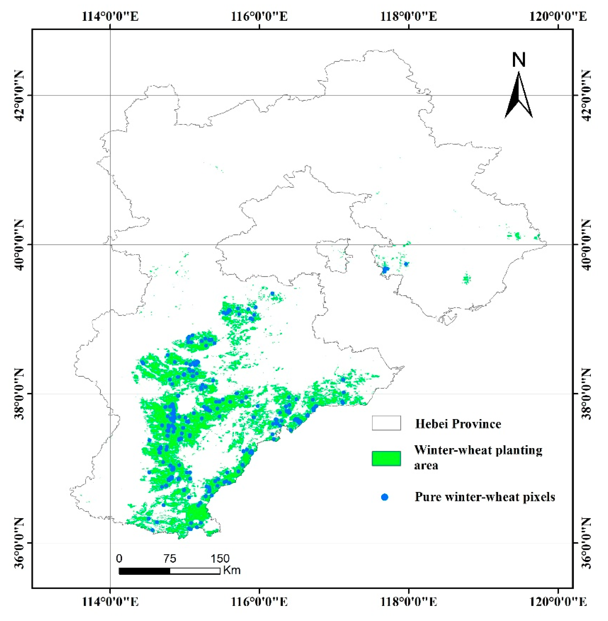
2.1. Study Area

The study area is located in Hebei Province in Northern China, between 36°05′ and 42°40′ N and between 113°27′ and 119°50′ E (Figure 1). Hebei Province contains plateaus, mountains, hills, and plains, with the latter accounting for 41.2% of the total area of the province. Hebei Province has a temperate continental monsoon climate, with cold and dry winters, dry and windy springs, hot and rainy summers, and clear and cool autumns. The province’s average annual rainfall is 350–815 mm, and its annual average temperature is (–0.3)–14.0 °C. The main local cultivation system is a double-season rotation, with winter wheat–corn rotation being the most common; other crops include cotton, spring corn, millet, and peanuts.

2.2. Data

2.2.1. Remote Sensing Data and Preprocessing

Remote sensing data were obtained from the Terra satellite daily surface reflectivity product MOD09GA, which is developed by the National Aeronautics and Space Administration (NASA) MODIS land product group (https://ladsweb.modaps.eosdis.nasa.gov, accessed on 26 June 2020). The product includes daily surface reflectance data from channels 1–7 with a spatial resolution of 500 m. The MODIS NDVI daily product was obtained from the red and near-infrared channels, and the maximum value of each five-day period was then taken to obtain the MODIS NDVI five-day composite products. A total of 31 NDVI composites from 01 February to 30 June 2018 were used in this study, which covers the key phenological growth stages of winter wheat, such as GUD, HD, and MD. To reduce the influence of noise on the NDVI time-series data, a Savitzky-Golay (S-G) [13,35,36] filter was applied to the whole time-series. In this study, the MODIS data were mainly used to determine the winter-wheat distribution and phenological phases.

2.2.2. Phenological Monitoring Station Data and Field Data

The phenological monitoring station data were obtained from the Meteorological Data Sharing Service System of China (http://data.cma.cn, accessed on 4 August 2020). This data set contains field records of crop growth and development since September 1991. The data include crop varieties, names, and dates of crop development stages, abnormal development stages, etc. Data from 15 phenological monitoring stations in Hebei Province were used (Figure 1b), each of which recorded the GUD, HD, and MD. The ground GUD was recorded by observers when more than half of the winter-wheat leaves had begun to turn green and reached a length of 1–2 cm in a wheat field near the station; the ground HD was recorded by observers when more than half of the top of the ear (excluding the awns) was exposed from the leaf sheath in a wheat field near the station; and the ground MD was recorded by observers when the endosperm of more than 50% of grains was waxy, and the ear and the node under the ear had turned yellow in a wheat field near the station. These data were used to verify the results for the phenological phases extracted using the TWDTW method. Additionally, we collected ground samples from field surveys in 2018. The location of each winter wheat sample was recorded using a mobile GPS device. Then, we added some non-winter-wheat samples (e.g., water, forest grass, town) through visual interpretation on the high-resolution image of Google Earth. Finally, 263 winter-wheat samples and 223 non-winter-wheat samples were collected. The samples were divided into two parts—one part used for training and classification, another part used for accuracy evaluation. (Figure 1b).

2.2.3. Temperature Data

The temperature data were based on European Space Agency (ESA) EAR5 data (https://cds.climate.copernicus.eu/, accessed on 16 August 2020). Data were acquired for latitudes between 35° and 45° N and longitudes between 112° and 120° E, covering the whole of Hebei Province. The grid intervals of longitude and latitude were both 0.1°. The EAR5 data provide one temperature measurement per hour, that is, 24 data sets every day. Data were obtained from 01 February to 30 June 2018, that is, for a total of 150 days. In this study, the temperature data were mainly used to analyze the effects of accumulated temperature on the winter-wheat phenological phases.

3. Methodology

3.1. Extraction of Winter Wheat Distribution by TWDTW Classification Method

The land cover sample points and MODIS NDVI time-series data were used to construct the NDVI time-series curve. The waveform of the time-series curve reflects the growth and changes of land cover types. According to the phenological characteristics of different land cover types, the winter wheat distribution was extracted using the TWDTW classification method.

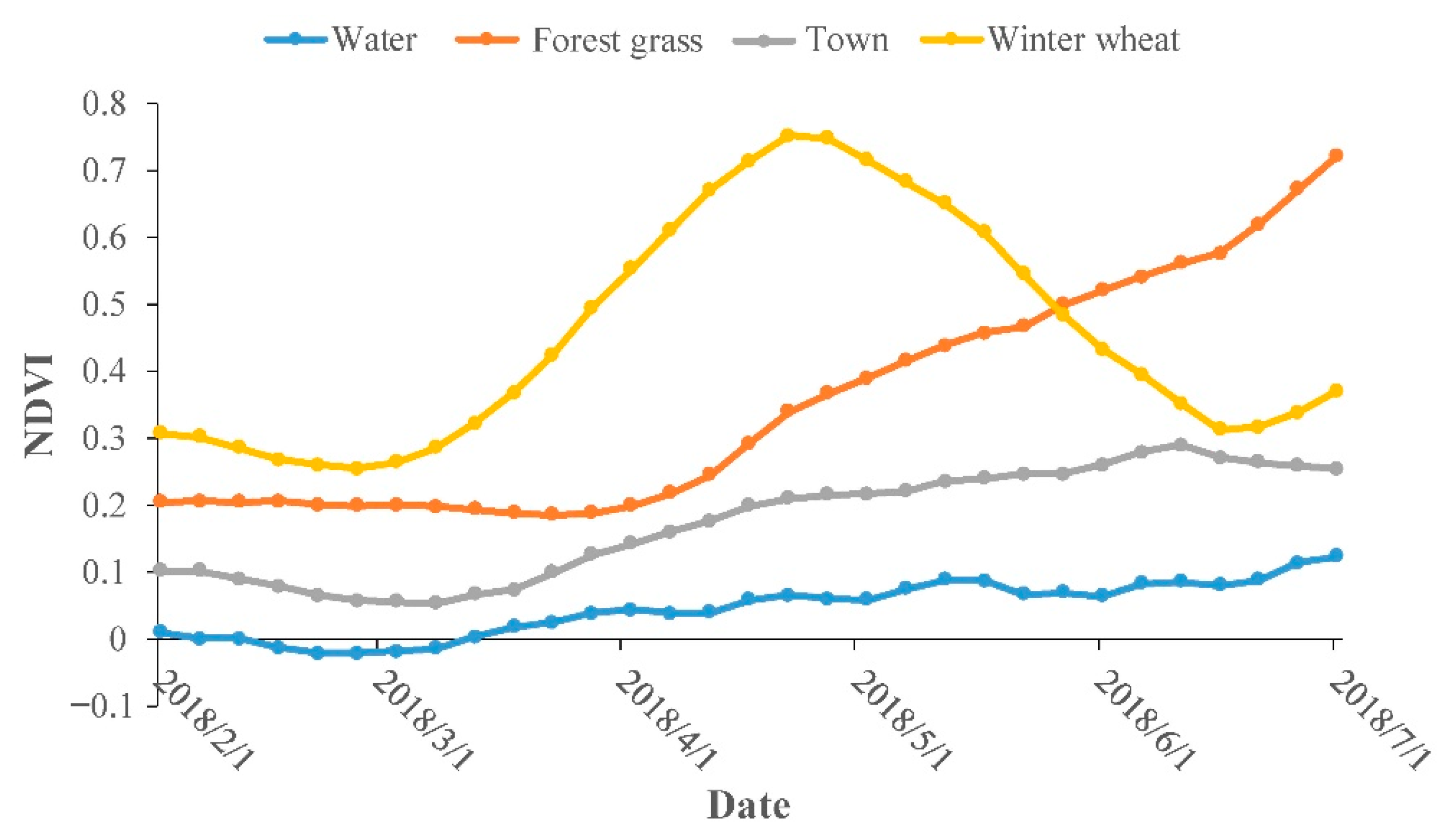
3.1.1. Phenological Characteristics of Land Cover

Different land cover types have different phenological patterns. Therefore, it is very important to understand the changes in the phenological characteristics of different land cover types [37]. During the growth period of winter wheat, the NDVI time-series curves of several typical land cover types are different from those of winter wheat. As shown in Figure 2, the NDVI of winter wheat is greater than the NDVI of non-vegetation land cover types (e.g., water, town). The NDVI of winter wheat gradually increased from March, peaked in May, then gradually decreased and reached the lowest value in mid-late June. In contrast, the NDVI of forest grass gradually increased from April and showed different phenological characteristics from winter wheat.

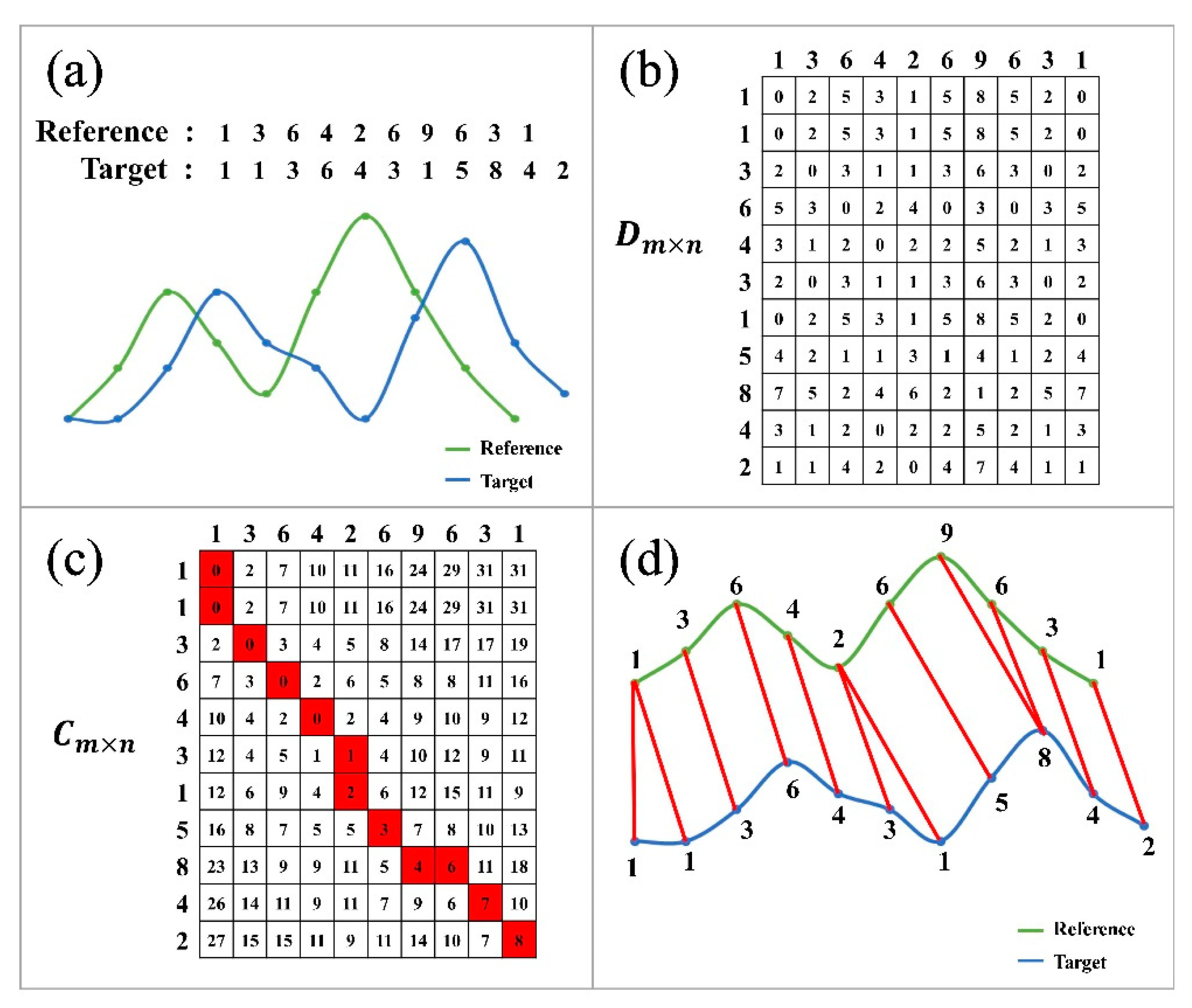
3.1.2. TWDTW Classification Method

The TWDTW algorithm includes a time weighting factor based on dynamic warping to find the path with the minimum cumulative distance. When calculating the degree of similarity between two sequences, it is important to consider not only the numerical size of the matching points, but also the period between the matching points to avoid a severe mismatch between sequences [32]. Suppose that there are two time-series curves: X = (X1, X2, X3, …, Xm), and Y = (Y1, Y2, Y3, …, Yn). First, the distance matrix of the two time-series D m × n [Equation (1)] (Figure 3b) is constructed, where each element in the matrix is defined as D i , j = w i , j X i Y j , where w i , j is the time weighting factor following a logistic function, as given in Equation (2). Secondly, the cumulative distance matrix C m × n [Equation (3)] (Figure 3c) is calculated.
D m × n = D 1 , 1 D 1 , 2 D 2 , 1 D 2 , 2 D 1 , n D 2 , n D m , 1 D m , 2 D m , n
w i , j = 1 1 + e α t i t j β
C i , j = D i , j + m i n C i 1 , j 1 , C i 1 , j ,   C i , j 1
where α and β represent the steepness and median value of the time-series [32].
Thirdly, the minimum distance between the two curves and the corresponding matching relationship is determined using the cumulative distance matrix C m × n (Figure 3c). According to this matching relationship, the time alignment relationship of the two curves is obtained (Figure 3d).
Specifically, winter wheat in Hebei province was mapped using the following steps: (1) One hundred and forty-two winter-wheat samples and one hundred and sixteen non-winter-wheat samples were randomly selected for training. One hundred and twenty-one winter-wheat samples and one hundred and seven non-winter-wheat samples were selected for validation; (2) the average winter-wheat phenological curve was generated using the NDVI time-series curve of 142 winter-wheat samples; (3) the TWDTW distance between the average winter-wheat phenological curve and the phenological curve of the training samples were calculated, and the best threshold 1.5 is obtained; (4) the TWDTW distance between the average winter-wheat phenological curve and all the NDVI time-series curves was calculated, and the samples whose distance was less than the threshold were considered to be winter wheat.

3.2. Determination of Winter-Wheat Key Phenological Phases by TWDTW Algorithm

Based on the MODIS NDVI time-series data and the winter-wheat distribution, the key phenological phases of winter wheat were determined, including the following steps: (a) The selection of pure winter-wheat pixels; (b) the definition of the average GUD, HD, and MD; (c) the waveform adjustment; (d) the calculation of the difference between each NDVI phenological curve and the average phenological curve using the TWDTW algorithm; and (e) the determination of the key winter-wheat phenological phases and accuracy assessment (Figure 4).

3.2.1. Selection of Pure Winter-Wheat Pixels

The accuracy of the average phenological curve directly affects the accuracy of the extraction of GUD, HD, and MD. In this study, large homogeneous areas of winter wheat were chosen to avoid mixed pixels, due to the coarser resolution of MODIS [38,39]. Using pure winter-wheat pixels to generate an average phenological curve can improve the accuracy of the extraction of GUD, HD, and MD. In this study, the coefficient of variation was used to obtain pure winter-wheat pixels [13]. The coefficient of variation, also known as the coefficient of dispersion, is defined as the ratio of the standard deviation to the mean. The steps in the process for the selection of pure winter-wheat pixels are as follows:
(1) Establish a series of 3 × 3 windows with each winter-wheat pixel as the center. (2) Calculate the coefficient of variation of each of the nine pixels in each 3 × 3 window. As the time range of the MODIS NDVI time-series data used in this paper is from 1 February to 30 June 2018, and the time interval is five days, there are 31 images in total, and 31 coefficients of variation can be obtained for each pixel. (3) If the 31 coefficients of variation of a given pixel are all less than the threshold of 0.5%, the winter-wheat pixel is determined to be a pixel of pure winter-wheat.
Here, we argue that it is appropriate to set the size of the window to 3 × 3, considering that the winter-wheat planting area in Hebei Province is mainly in the plain area, and the wheat is planted continuously. If the window is too large, it is likely to be affected by mixed pixels, and no pure winter-wheat pixels can be found. Additionally, the threshold value of 0.5% was chosen—since, if the threshold value is too large, the influence of mixed pixels cannot be effectively removed; in contrast, if the threshold is too small, too few pixels of pure winter-wheat are extracted, which is not representative.

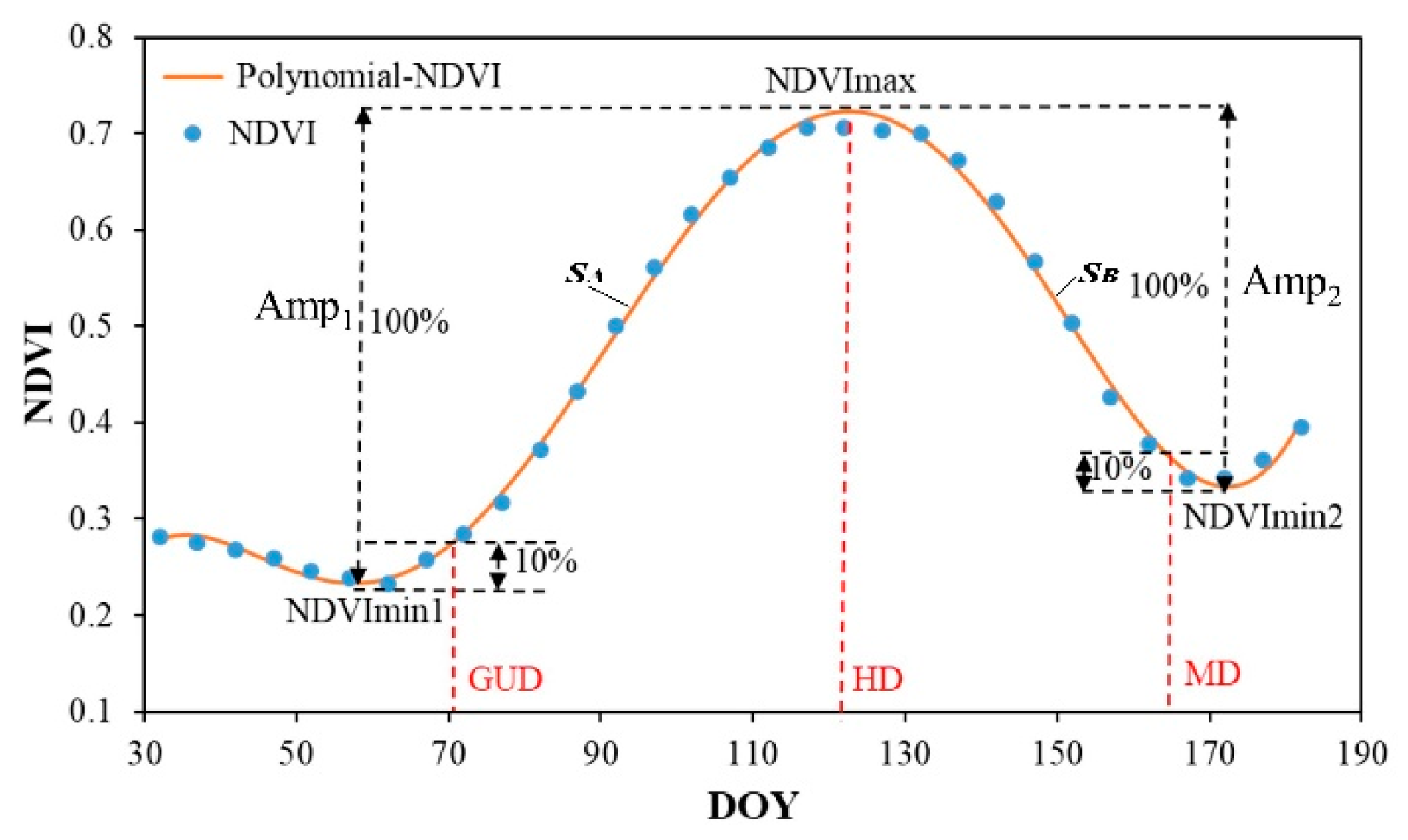
3.2.2. Definition of the Average GUD, HD, and MD

Based on the extracted pure winter-wheat pixels, the average winter-wheat phenological curve was obtained using the arithmetic average, which is used to define the average of GUD, HD, and MD. Since the average winter-wheat phenological curve is a time-series with a 5-day interval, a 6th-order polynomial function was used to fit the 5-day interval NDVI time-series and reconstruct daily NDVI time-series; this approach has previously been used to extract crop phenology [19,21,22,23]. Here, the GUD and MD were defined using the relative threshold method [13,24,35], and the HD was defined via the maximum method [35]. The definition of the average GUD, HD, and MD is as shown in Figure 5.

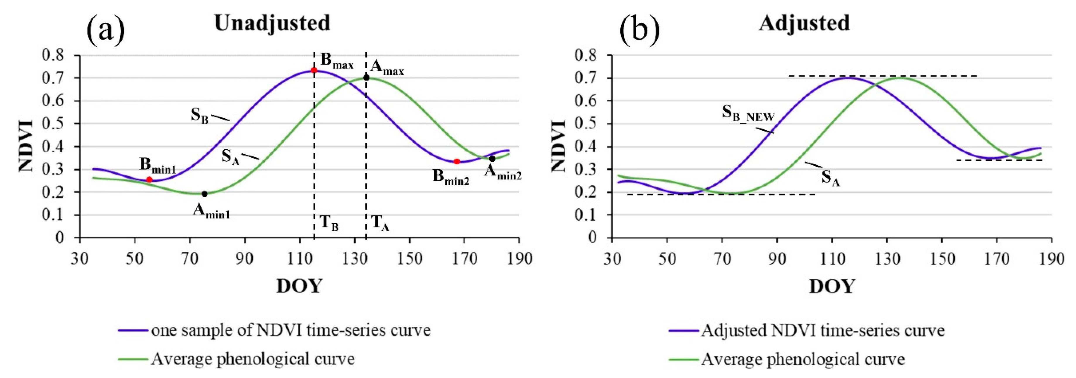
3.2.3. Waveform Adjustment

Before extracting the differences between each NDVI phenological curve and the average phenological curve, it is necessary to preprocess the phenological curve of winter wheat, including waveform adjustment and polynomial fitting. Due to factors, such as temperature, latitude, and longitude, and the NDVI value of winter wheat, may be different in different regions even for the same phenological phase. For example, in some regions, when winter wheat enters the HD, the NDVI reaches 0.8, while in other regions, the NDVI only reaches 0.7. Therefore, it was necessary to adjust the NDVI time-series curve to reduce the influence of different amplitudes on the two phenological curves. Details of the waveform adjustment method are given in Appendix A.

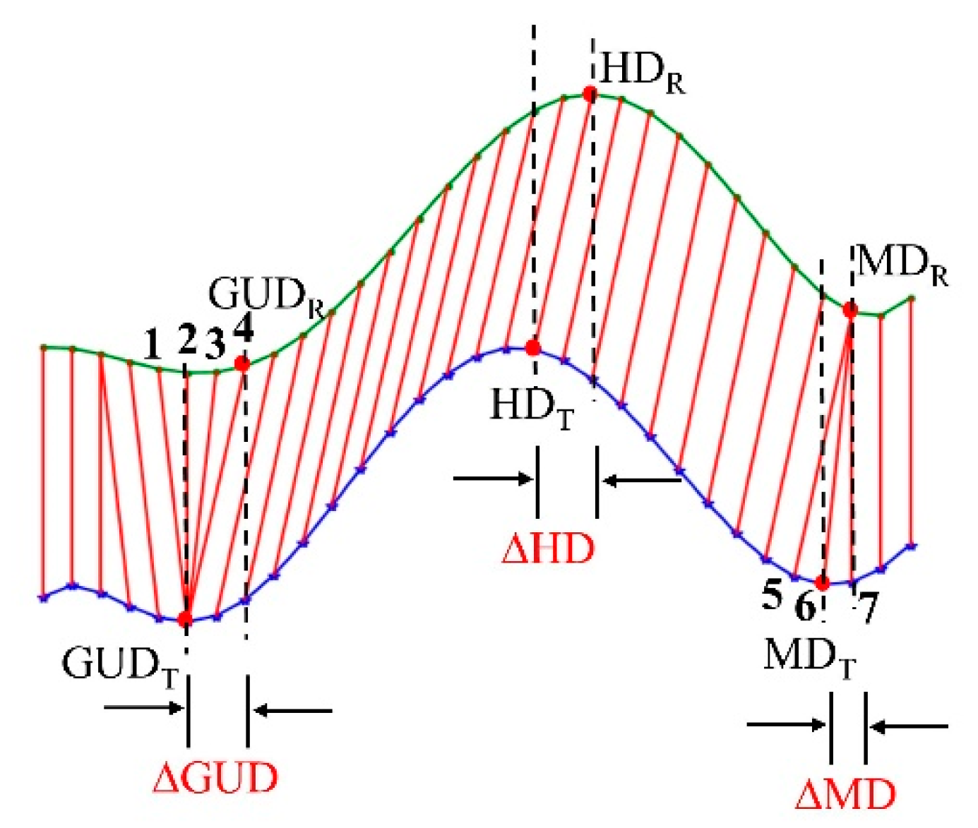
3.2.4. Calculation of the Difference between NDVI Phenological Curves and the Average Phenological Curve

According to the time alignment relationship by the TWDTW algorithm in Section 3.1.2, when the phenological phase of the reference curve is known, the phenological phase of the target curve can be obtained. Figure 6 shows an example of how the TWDTW algorithm was used to determine the phenological phase. Two NDVI phenological curves were used, namely, a reference curve and a target curve, where the key phenological phases (GUD, HD, and MD) of the reference curve (termed GUDR, HDR, and MDR, respectively) are known. Three cases are analyzed here. In the first case, one point on the reference curve matches one point on the target curve; HDR and the location of HD on the target curve (HDT) belong to this situation; that is, there is only one line segment connecting HDR and HDT. This shows that, from the perspective of waveform similarity, HDT has similar characteristics to HDR, so HDT can be regarded as the HD of the target curve. In the second case, multiple points on the reference curve match one point on the target curve; GUDR and the location of GUD on the target curve (GUDT) belong to this situation. GUDR and the three points on the left match the GUDT point. From the perspective of alignment, although GUDT is aligned with four points, GUDR only matches GUDT, so GUDT can be regarded as the GUD of the target curve. In the third case, one point on the reference matches multiple points on the target curve; this is the case for MDR and the location of MD on the target curve (MDT). MDR is aligned with three points on the target curve. In this case, the average point is chosen as the MD of the target curve. After the phenological phase of the target curve is determined, the difference between each NDVI phenological curve and the average phenological curve can be calculated by Equation (4).
Phenological   difference = n   ×   T #
where n represents the number of points between the corresponding phenological phases of the reference curve and the target curve, and T represents the temporal resolution of the phenological curve.

3.2.5. Determination of GUD, HD, and MD

When the differences between each NDVI phenological curve and the average phenological curve (∆GUD, ∆HD, and ∆MD) were calculated, combined with the known average phenological phases. The phenological phases of the target curve were obtained according to Equations (5)–(7).
GUD T = GUD R + GUD
HD T = HD R + HD
MD T = MD R + MD
Using the same method, the GUD, HD, and MD were obtained for each winter-wheat NDVI phenological curve.

3.3. Accuracy Assessment

The coefficient of determination (R2), root mean square error (RMSE), and bias were used to assess the accuracy of the values of GUD, HD, and MD. These metrics are defined as follows:
R 2 = i = 1 n y i y ¯ 2 i = 1 n y i y ¯ 2
RMSE = 1 n i = 1 n y i y i 2
bias = 1 n i = 1 n y i y i
where n represents the number of samples, y i represents the ground-observed phenological phase,   y i represents the satellite-derived phenological phase, and y ¯ represents the average phenological phase.

4. Results

4.1. Winter Wheat Distribution and Pure Winter-Wheat Pixels

The TWDTW method was used to extract winter wheat distribution in the Hebei area, and the result is shown in Figure 7. It can be seen from the figure that winter wheat in Hebei is mainly distributed in the central and southern plains of Hebei Province, and a small amount of cultivation is in the northeastern region of Hebei Province. Using 121 winter wheat and 107 non-winter wheat verification samples to verify the accuracy of the extraction results. The overall accuracy of the classification is 94.74%, and the kappa coefficient is 0.90. According to the winter-wheat area obtained by the TWDTW classification method, the area of winter wheat in Hebei Province in 2018 was found to be 2.5 million hectares, which is close to the value of 2.3 million hectares published in the Yearbook of Hebei Province 2018. Additionally, a total of 338 pure winter-wheat pixels were extracted (Figure 7). These pure winter-wheat pixels were used to generate the average phenological curve and analyze the spatial patterns of the phenological phases.

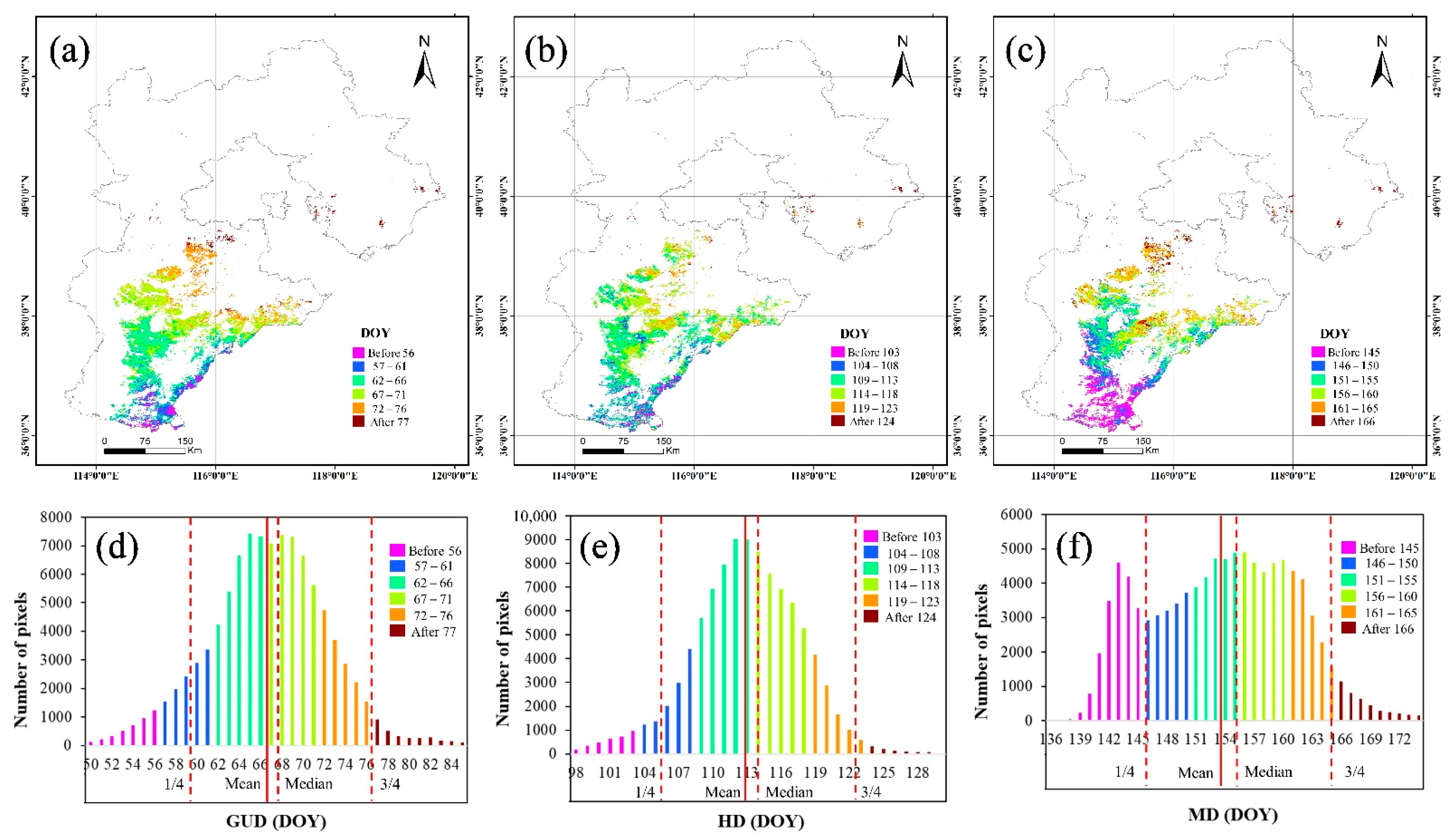
4.2. Spatial Patterns of GUD, HD, and MD

Based on the distribution of winter wheat, the TWDTW algorithm was used to extract three key phenological phases (GUD, HD, and MD) of winter wheat during the growth period in Hebei Province in 2018. The results for the GUD, HD, and MD are shown in Figure 8a–c, respectively, and the corresponding frequency distributions are shown in Figure 8d–f, respectively. The GUD, HD, and MD all differ significantly between the south and north of Hebei Province. The GUD ranges from Day of Year (DOY) 50 (19 February) to DOY 84 (25 March), mainly from DOY 59 (28 February) to DOY 76 (17 March), and the average GUD is DOY 67 (8 March). The HD ranges from DOY 98 (8 April) to DOY 128 (8 May), mainly from DOY 104 (14 April) to DOY 123 (3 May), and the average HD is DOY 113 (23 April). The MD ranges from DOY 136 (16 May) to DOY 172 (21 June), mainly from DOY 146 (26 May) to DOY 165 (14 June), and the average MD is DOY 154 (3 June).

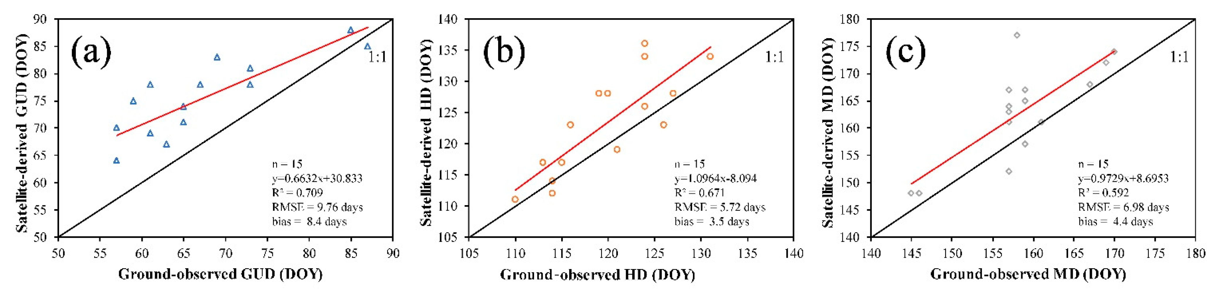
4.3. Validation of the Extracted GUD, HD, and MD

As shown in Figure 9, the results of the phenological phase extraction were verified using the GUD, HD, and MD observed at 15 phenological monitoring stations. From Figure 9a, it can be seen that the phenological phase obtained by the TWDTW method is significantly correlated with the ground-observed phenological phase, with an R2 greater than 0.59. The GUD has the highest R2 of 0.71, while the MD has the lowest R2 of 0.59. For the RMSE and bias, the HD has the smallest values of 5.72 days and 3.5 days, respectively, while the GUD has the largest values of 9.76 days and 8.4 days, respectively. As can be seen in Figure 9, the TWDTW method overestimates the GUD, HD, and MD. Accordingly, using the TWDTW method to extract the phenological phase has high accuracy and performs best for the HD.

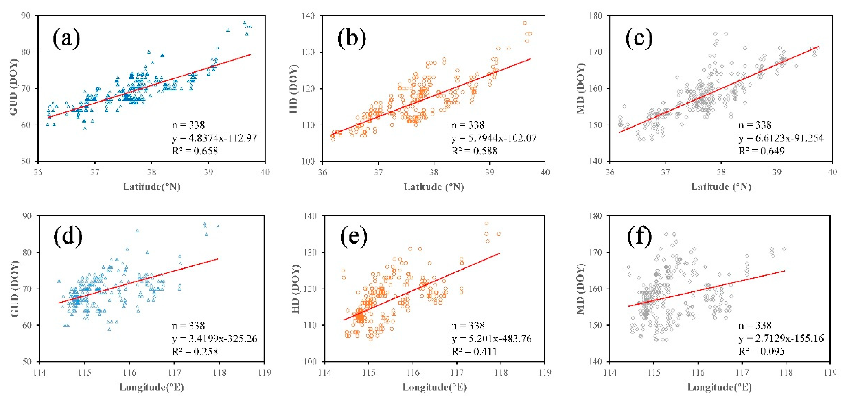
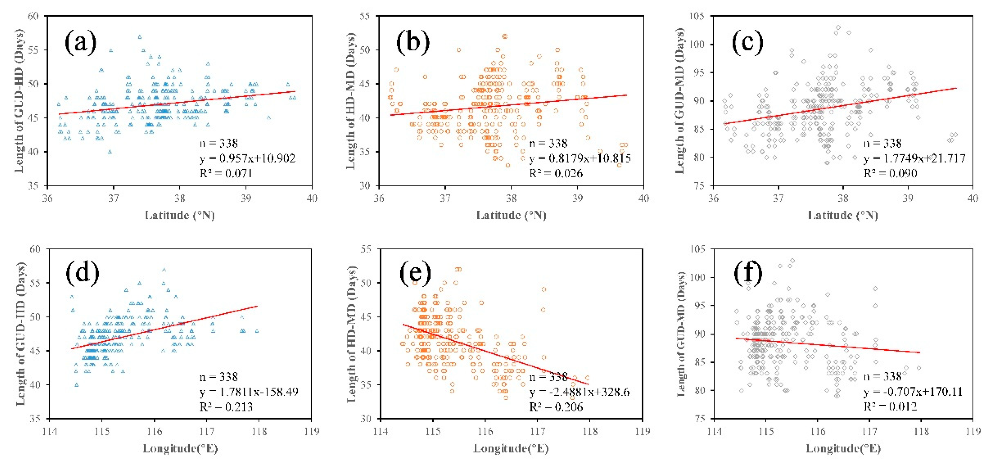
4.4. Relationship between Winter-Wheat Phenology Pattern and Geographical Location

To investigate the distribution pattern of winter-wheat phenological phases, we analyzed the changes in the distribution of the main phenological phases of winter-wheat in Hebei Province with longitude and latitude. The results are shown in Figure 10. From this figure, it can be seen that the GUD, HD, and MD have a high correlation with latitude, with R2 values of 0.658, 0.588, and 0.649, respectively. By establishing a linear regression equation, it was found that for each 1° increase in latitude, the GUD, HD, and MD are delayed by 4.84, 5.79, and 6.61 days, respectively (see Figure 10a–c, respectively). The R2 values of the GUD, HD, MD, with longitude are 0.258, 0.411, and 0.095, respectively (Figure 10d–f, respectively). The HD has the strongest correlation with longitude. According to the regression equation, for each 1° increase in longitude, the HD is delayed by 5.2 days. The correlation between MD and longitude is the weakest, with an R2 of only 0.095, indicating that MD does not change with longitude.
To further analyze the influence of latitude and longitude on the phenological phases, the length of time between the GUD and HD (GUD-HD), between the HD and MD (HD-MD), and between the GUD and MD (GUD-MD) were extracted, and the relationships between these lengths and latitude and longitude were analyzed. The results are shown in Figure 11. As shown in the figure, the R2 values between GUD-HD, HD-MD, and GUD-MD, and latitude are 0.071, 0.026, and 0.090, respectively (Figure 11a–c, respectively), which shows that the length of time between phenological phases varies little with latitude. Meanwhile, the R2 values between GUD-HD, HD-MD, and GUD-MD, and longitude are also very small, namely, 0.213, 0.206, and 0.012, respectively (Figure 11d–f, respectively). This shows that the length of time between phenological phases varies little with longitude. The results show that the influence of longitude is greater than that of latitude on GUD-HD and HD-MD. In summary, changes in latitude and longitude impact the dates of the phenological phases, which is mainly due to the difference in temperature. As the latitude and longitude increase, the phenological phases are delayed, with latitude playing a larger role than longitude. However, latitude and longitude have little effect on the lengths of the phenological phases; across the study area, the lengths of time between GUD and HD, HD and MD, and GUD and MD are stable at 46, 41, and 87 days, respectively.

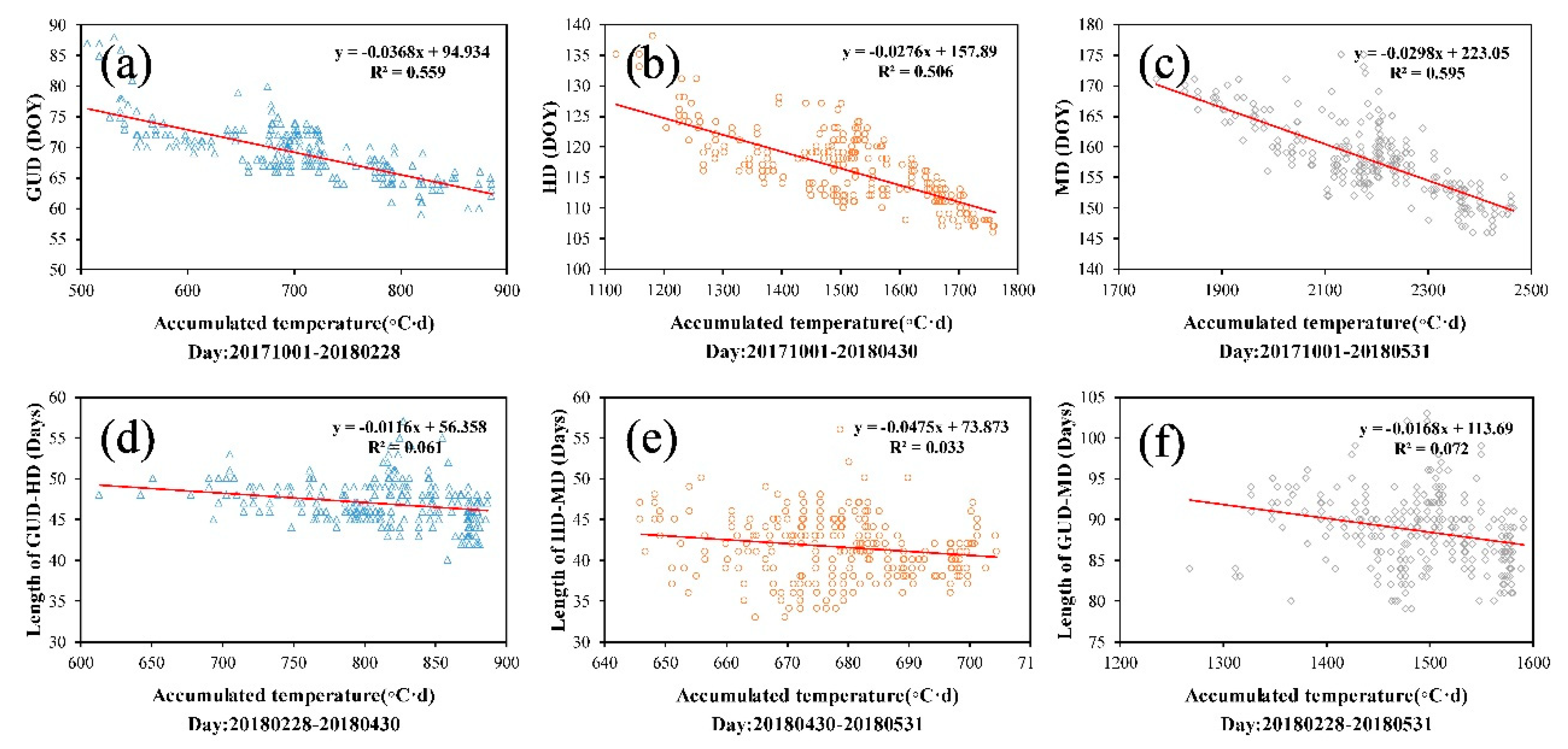
4.5. Relationship between Winter-Wheat Phenology Pattern and Accumulated Temperature

In Hebei Province, winter wheat is generally sown in October, the GUD typically occurs at the end of February or early March of the following spring, the HD typically occurs at the end of March or the beginning of April, and the MD typically occurs at the end of May or early June. Therefore, the accumulated temperature was calculated from 01 October 2017 onwards: From 01 October 2017 to 28 February 2018 for the GUD; from 01 October 2017 to 30 April 2018 for the HD; and from 01 October 2017 to 31 May 2018 for the MD. The accumulated temperature between the GUD and HD is the accumulated temperature of the HD minus that of the GUD—that is, the accumulated temperature between 28 February and 30 April 2018. The accumulated temperature between the HD and MD was calculated between 30 April and 31 May 2018. The accumulated temperature between the GUD and MD was calculated between 28 February and 31 May 2018. By analyzing the relationships between the accumulated temperature and phenological phases, it was found that the correlations between the accumulated temperature and phenological phases are relatively high; the R2 values between the GUD, HD, and MD, and the accumulated temperature in the corresponding period were 0.559, 0.506, and 0.595, respectively (Figure 12a–c, respectively). The results showed that, with the decrease of accumulated temperature, the phenological phase is delayed. From Figure 12d–f, it can be seen that the correlation coefficients between the lengths of the phenological phases and the corresponding accumulated temperature are very low, with R2 values of only 0.061, 0.033, and 0.072 for GUD, HD, and MD, respectively.

5. Discussion

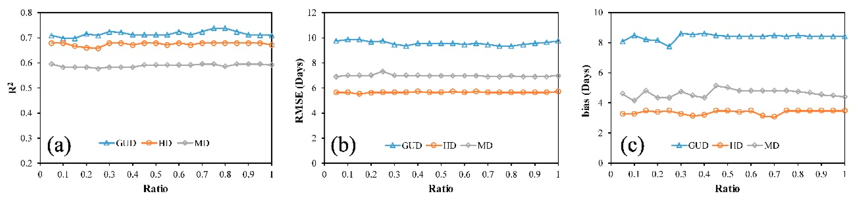
5.1. Impact of the Calculation Method of the Average Phenological Curve on the Verification Results

Because the methods proposed in this paper involve using the average phenological curve and the target curve to calculate the difference between each NDVI phenological curve and the average phenological curve and extract the phenological phases, the average phenological curve will directly affect the accuracy of the results. Therefore, to analyze the influence of the calculation method for the average phenological curve on the accuracy of the phenological phase extraction, we calculated the average phenological curve using different randomly selected fractions of the 338 pure winter-wheat samples for sample sizes between 5 and 100% with a 5% increment (i.e., 5%, 10%, 15%, …, 100%; that is, a total of 20 sample sizes) and used these average phenological curves to extract the GUD, HD, and MD using the TWDTW algorithm. The results are shown in Figure 13. As can be seen in the figure, changing the sample size had little effect on the R2, RMSE, and bias; for the GUD, HD, and MD, the R2 was stable at about 0.7, 0.68, and 0.6, respectively; the RMSE remained stable at around 9.7, 5.7, and 7.0 days, respectively; and the bias was stable at around 8.4, 3.4, and 4.6 days, respectively.
The above analysis suggests that using different numbers of winter-wheat samples to generate the average phenological curve has little effect on the results.

5.2. Comparison with Other Methods

To further verify the performance and advantages of using the TWDTW algorithm to extract winter-wheat phenology, several other methods were also used to extract the GUD, HD, and MD of winter wheat. These methods were the RT10 and RT20 thresholding methods and a method involving the maximum of the curvature change rate of the fitted logistic curve (CCRmax) [13]; RT10 and RT20 are typical dynamic thresholding methods and RT10 and RT20 is a change detection method. The method of extracting HD uses the maximum method [35]. The method of extracting MD uses the RT10 method [24].
We compared the results of the phenological extraction using the TWDTW algorithm with those using the RT10, RT20, and CCRmax methods, as illustrated in Figure 14. Compared with the other methods, in terms of R2, the TWDTW algorithm does not offer a notable advantage (Figure 14a). For the GUD, the TWDTW algorithm is slightly better than the RT20 and CCRMAX methods, and slightly inferior to the RT10 method. For the HD, the performance of the TWDTW algorithm is similar to that of the CCRMAX method. For the MD, the TWDTW algorithm performs better than the RT10 method. However, from the perspective of the RMSE and bias (Figure 14b,c, respectively), for the GUD, the performance of the TWDTW algorithm is similar to those of the RT10 and CCRMAX methods and significantly better than that of the RT20 method. That is, for the HD and MD, the TWDTW algorithm is significantly better than the CCRMAX and RT10 methods, respectively.

6. Conclusions

In this paper, we proposed a novel phenological phase determination method based on the TWDTW algorithm using MODIS NDVI time-series data. The advantages of the TWDTW algorithm are as follows: (1) Based on extracted pure winter-wheat pixels, an average phenological curve is generated, which can effectively reduce the influence of mixed pixels; (2) the algorithm completes the time alignment of the entire growth period and can extract GUD, HD, and MD simultaneously. The phenological phase extraction using the TWDTW algorithm was found to have high accuracy. In terms of verification accuracy, the RMSEs of the GUD, HD, and MD were 9.76, 5.72, and 6.98 days, respectively. Additionally, the proposed TWDTW method was also demonstrated to perform better than several other methods. Furthermore, it was shown that, in Hebei Province, the GUD, HD, and MD are mainly affected by latitude and accumulated temperature; as the latitude increases from south to north, the GUD, HD, and MD are delayed. For each 1° rise in latitude, the GUD, HD, and MD are delayed by 4.84, 5.79, and 6.61 days, respectively. The higher the accumulated temperature, the earlier the phenological phases occurred. However, the latitude and accumulated temperature had little effect on the length of the phenological phases. Throughout Hebei Province, the lengths of time between GUD and HD, HD and MD, and GUD and MD were stable at 46, 41, and 87 days, respectively. The phenological phase extraction method proposed in this paper can be applied to other crops and can support crop field management and policy-making.

Author Contributions

Conceptualization, F.Z. and G.Y.; data curation, F.Z., Y.Z., and S.H.; methodology, G.Y. and X.Y.; formal analysis, H.Y., H.C., and Y.H.; writing—original draft preparation, F.Z.; writing—review and editing, G.Y. and C.Z. All authors have read and agreed to the published version of this manuscript.

Funding

This research was funded by the Key-Area Research and Development Program of Guangdong Province (Nos. 2019B020214002 and 2019B020216001), the Beijing Million Talent Project (No. 2019A10), and the National Key Research and Development Program of China (No. 2017YFE0122500).

Data Availability Statement

The Remote sensing data were obtained from the Terra satellite daily surface reflectivity product MOD09GA, which is developed by the National Aeronautics and Space Administration (NASA) MODIS land product group (https://ladsweb.modaps.eosdis.nasa.gov, accessed on 26 June 2020). The phenological monitoring station data were obtained from the Meteorological Data Sharing Service System of China (http://data.cma.cn, accessed on 4 August 2020). The temperature data were based on European Space Agency (ESA) EAR5 data (https://cds.climate.copernicus.eu/, accessed on 16 August 2020).

Acknowledgments

We thank three reviewers and editors for their invaluable comments and suggestions on the manuscript.

Conflicts of Interest

The authors declare no conflict of interest.

Appendix A

Waveform Adjustment Method

The waveform adjustment method involves stretching the amplitude of the sample phenological curve so that the maximum and minimum values of the curve are the same as on the average phenological curve. The steps of the waveform adjustment process are as follows: (1) The average phenological curve SA(t) and the sample phenological curve SB(t) are divided into two parts according to the maximum value of the curve. The expressions for SA(t) and SB(t) are given in Equations (A1) and (A2), respectively, where the start and end days of year (DOYs) for both SA(t) and SB(t) are 32 and 186, respectively; and TA and TB represent the DOYs corresponding to the maximum values of SA(t) and SB(t), respectively; (2) Through Equation (A3), we can obtain SB_NEW(t), as shown in Figure A1a. The results of the waveform adjustment are shown in Figure A1b.
S A ( t ) = S A 1   ( t )         32 t T A   S A 2   t         T A < t 186
S B ( t ) =   S B 1   ( t )         32 t T B S B 2   ( t )         T B < t 186
S B _ NEW ( t ) =   S B 1 ( t ) A max - A min 1 B max - B min 1 + A max -   B max A max - A min 1 B max - B min 1         32 t T A   S B 2 ( t ) A max - A min 2 B max - B min 2 + A max -   B max A max - A min 2 B max - B min 2         T A < t 186
where Bmax represents the maximum of SB(t), and Bmin1 and Bmin2 represent the minimum of SB1(t) and SB2(t), respectively. Amax represents the maximum value of SA(t), and Amin1 and Amin2 represent the minimum value of SA1(t)and SA2(t), respectively.
Figure A1. A comparison of the NDVI time-series curve and the average phenological curve before (a) and after (b) waveform adjustment.
Remotesensing 13 01836 g0a1

References

  1. Franch, B.; Vermote, E.F.; Becker-Reshef, I.; Claverie, M.; Huang, J.; Zhang, J.; Justice, C.; Sobrino, J.A. Improving the timeliness of winter wheat production forecast in the United States of America, Ukraine and China using MODIS data and NCAR Growing Degree Day information. Remote Sens. Environ. 2015, 161, 131–148. [Google Scholar] [CrossRef]
  2. Zeng, L.L.; Wardlow, B.D.; Xiang, D.X.; Hu, S.; Li, D.R. A review of vegetation phenological metrics extraction using time-series, multispectral satellite data. Remote Sens. Environ. 2020, 237, 111511. [Google Scholar] [CrossRef]
  3. Atkinson, P.M.; Jeganathan, C.; Dash, J.; Atzberger, C. Inter-comparison of four models for smoothing satellite sensor time-series data to estimate vegetation phenology. Remote Sens. Environ. 2012, 123, 400–417. [Google Scholar] [CrossRef]
  4. Guyon, D.; Guillot, M.; Vitasse, Y.; Cardot, H.; Hagolle, O.; Delzon, S.; Wigneron, J.P. Monitoring elevation variations in leaf phenology of deciduous broadleaf forests from SPOT/VEGETATION time-series. Remote Sens. Environ. 2011, 115, 615–627. [Google Scholar] [CrossRef]
  5. Hou, X.H.; Gao, S.; Niu, Z.; Xu, Z.G. Extracting grassland vegetation phenology in North China based on cumulative SPOT-VEGETATION NDVI data. Int. J. Remote Sens. 2014, 35, 3316–3330. [Google Scholar] [CrossRef]
  6. Pan, Z.K.; Huang, J.F.; Zhou, Q.B.; Wang, L.M.; Cheng, Y.X.; Zhang, H.K.; Blackburn, G.A.; Yan, J.; Liu, J.H. Mapping crop phenology using NDVI time-series derived from HJ-1 A/B data. Int. J. Appl. Earth Obs. 2015, 34, 188–197. [Google Scholar] [CrossRef] [Green Version]
  7. Wu, C.Y.; Peng, D.L.; Soudani, K.; Siebicke, L.; Gough, C.M.; Arain, M.A.; Bohrer, G.; Lafleur, P.M.; Peichl, M.; Gonsamo, A.; et al. Land surface phenology derived from normalized difference vegetation index (NDVI) at global FLUXNET sites. Agr. Forest Meteorol. 2017, 233, 171–182. [Google Scholar] [CrossRef]
  8. Verhegghen, A.; Bontemps, S.; Defourny, P. A global NDVI and EVI reference data set for land-surface phenology using 13 years of daily SPOT-VEGETATION observations. Int. J. Remote Sens. 2014, 35, 2440–2471. [Google Scholar] [CrossRef] [Green Version]
  9. Wang, C.; Li, J.; Liu, Q.H.; Zhong, B.; Wu, S.L.; Xia, C.F. Analysis of Differences in Phenology Extracted from the Enhanced Vegetation Index and the Leaf Area Index. Sens. Basel 2017, 17, 1982. [Google Scholar] [CrossRef] [PubMed] [Green Version]
  10. Yang, Y.T.; Guan, H.D.; Shen, M.G.; Liang, W.; Jiang, L. Changes in autumn vegetation dormancy onset date and the climate controls across temperate ecosystems in China from 1982 to 2010. Global Change Biol. 2015, 21, 652–665. [Google Scholar] [CrossRef]
  11. Yang, Y.P.; Luo, J.C.; Huang, Q.T.; Wu, W.; Sun, Y.W. Weighted Double-Logistic Function Fitting Method for Reconstructing the High-Quality Sentinel-2 NDVI Time Series Data Set. Remote Sens. Basel 2019, 11, 2342. [Google Scholar] [CrossRef] [Green Version]
  12. Vrieling, A.; Skidmore, A.K.; Wang, T.J.; Meroni, M.; Ens, B.J.; Oosterbeek, K.; O’Connor, B.; Darvishzadeh, R.; Heurich, M.; Shepherd, A.; et al. Spatially detailed retrievals of spring phenology from single-season high-resolution image time series. Int. J. Appl. Earth Obs. 2017, 59, 19–30. [Google Scholar] [CrossRef]
  13. Gan, L.Q.; Cao, X.; Chen, X.H.; Dong, Q.; Cui, X.H.; Chen, J. Comparison of MODIS-based vegetation indices and methods for winter wheat green-up date detection in Huanghuai region of China. Agr. Forest Meteorol. 2020, 288, 108019. [Google Scholar] [CrossRef]
  14. Zhang, X.Y.; Friedl, M.A.; Schaaf, C.B.; Strahler, A.H.; Hodges, J.C.F.; Gao, F.; Reed, B.C.; Huete, A. Monitoring vegetation phenology using MODIS. Remote Sens. Environ. 2003, 84, 471–475. [Google Scholar] [CrossRef]
  15. Wu, C.Y.; Hou, X.H.; Peng, D.L.; Gonsamo, A.; Xu, S.G. Land surface phenology of China’s temperate ecosystems over 1999-2013: Spatial-temporal patterns, interaction effects, covariation with climate and implications for productivity. Agr. Forest Meteorol. 2016, 216, 177–187. [Google Scholar] [CrossRef]
  16. Cao, R.Y.; Chen, J.; Shen, M.G.; Tang, Y.H. An improved logistic method for detecting spring vegetation phenology in grasslands from MODIS EVI time-series data. Agr. Forest Meteorol. 2015, 200, 9–20. [Google Scholar] [CrossRef]
  17. Fisher, J.I.; Mustard, J.F.; Vadeboncoeur, M.A. Green leaf phenology at Landsat resolution: Scaling from the field to the satellite. Remote Sens. Environ. 2006, 100, 265–279. [Google Scholar] [CrossRef]
  18. Elmore, A.J.; Guinn, S.M.; Minsley, B.J.; Richardson, A.D. Landscape controls on the timing of spring, autumn, and growing season length in mid-Atlantic forests. Global Change Biol. 2012, 18, 656–674. [Google Scholar] [CrossRef] [Green Version]
  19. Jeong, S.J.; Ho, C.H.; Gim, H.J.; Brown, M.E. Phenology shifts at start vs. end of growing season in temperate vegetation over the Northern Hemisphere for the period 1982-2008. Global Change Biol. 2011, 17, 2385–2399. [Google Scholar] [CrossRef]
  20. Liu, L.L.; Zhang, X.Y.; Yu, Y.Y.; Guo, W. Real-time and short-term predictions of spring phenology in North America from VIIRS data. Remote Sens. Environ. 2017, 194, 89–99. [Google Scholar] [CrossRef]
  21. Piao, S.L.; Fang, J.Y.; Zhou, L.M.; Ciais, P.; Zhu, B. Variations in satellite-derived phenology in China’s temperate vegetation. Global Change Biol. 2006, 12, 672–685. [Google Scholar] [CrossRef]
  22. Yang, G.; Shen, H.F.; Zhang, L.P.; He, Z.Y.; Li, X.H. A Moving Weighted Harmonic Analysis Method for Reconstructing High-Quality SPOT VEGETATION NDVI Time-Series Data. IEEE Trans. Geosci. Remote 2015, 53, 6008–6021. [Google Scholar] [CrossRef]
  23. Cong, N.; Piao, S.L.; Chen, A.P.; Wang, X.H.; Lin, X.; Chen, S.P.; Han, S.J.; Zhou, G.S.; Zhang, X.P. Spring vegetation green-up date in China inferred from SPOT NDVI data: A multiple model analysis. Agr. Forest Meteorol. 2012, 165, 104–113. [Google Scholar] [CrossRef]
  24. Jonsson, P.; Eklundh, L. TIMESAT—A program for analyzing time-series of satellite sensor data. Comput. Geosci. UK 2004, 30, 833–845. [Google Scholar] [CrossRef] [Green Version]
  25. Lu, L.L.; Wang, C.Z.; Guo, H.D.; Li, Q.T. Detecting winter wheat phenology with SPOT-VEGETATION data in the North China Plain. Geocarto. Int. 2014, 29, 244–255. [Google Scholar] [CrossRef]
  26. Sakoe, H.; Chiba, S. Dynamic Programming Algorithm Optimization for Spoken Word Recognition. IEEE Trans. Acoust. Speech Signal Process. 1978, 26, 43–49. [Google Scholar] [CrossRef] [Green Version]
  27. Petitjean, F.; Inglada, J.; Gancarski, P. Satellite Image Time Series Analysis Under Time Warping. IEEE Trans. Geosci. Remote 2012, 50, 3081–3095. [Google Scholar] [CrossRef]
  28. Xue, Z.H.; Du, P.J.; Feng, L. Phenology-Driven Land Cover Classification and Trend Analysis Based on Long-term Remote Sensing Image Series. IEEE J. Stars 2014, 7, 1142–1156. [Google Scholar] [CrossRef]
  29. Petitjean, F.; Weber, J. Efficient Satellite Image Time Series Analysis Under Time Warping. IEEE Geosci. Remote Sens. Lett. 2014, 11, 1143–1147. [Google Scholar] [CrossRef]
  30. Guan, X.D.; Huang, C.; Liu, G.H.; Meng, X.L.; Liu, Q.S. Mapping Rice Cropping Systems in Vietnam Using an NDVI-Based Time-Series Similarity Measurement Based on DTW Distance. Remote Sens. 2016, 8, 19. [Google Scholar] [CrossRef] [Green Version]
  31. Costa, W.S.; Fonseca, L.M.G.; Korting, T.S.; Bendini, H.D.; de Souza, R.C.M. Spatio-Temporal Segmentation Applied to Optical Remote Sensing Image Time Series. IEEE Geosci. Remote Sens. Lett. 2018, 15, 1299–1303. [Google Scholar] [CrossRef]
  32. Maus, V.; Camara, G.; Cartaxo, R.; Sanchez, A.; Ramos, F.M.; de Queiroz, G.R. A Time-Weighted Dynamic Time Warping Method for Land-Use and Land-Cover Mapping. IEEE J. Stars 2016, 9, 3729–3739. [Google Scholar] [CrossRef]
  33. Belgiu, M.; Csillik, O. Sentinel-2 cropland mapping using pixel-based and object-based time-weighted dynamic time warping analysis. Remote Sens. Environ. 2018, 204, 509–523. [Google Scholar] [CrossRef]
  34. Cheng, K.; Wang, J.L. Forest-Type Classification Using Time-Weighted Dynamic Time Warping Analysis in Mountain Areas: A Case Study in Southern China. Forests 2019, 10, 1040. [Google Scholar] [CrossRef] [Green Version]
  35. Chu, L.; Liu, Q.S.; Huang, C.; Liu, G.H. Monitoring of winter wheat distribution and phenological phases based on MODIS time-series: A case study in the Yellow River Delta, China. J. Integr. Agr. 2016, 15, 2403–2416. [Google Scholar] [CrossRef]
  36. Liu, Z.J.; Wu, C.Y.; Liu, Y.S.; Wang, X.Y.; Fang, B.; Yuan, W.P.; Ge, Q.S. Spring green-up date derived from GIMMS3g and SPOT-VGT NDVI of winter wheat cropland in the North China Plain. ISPRS J. Photogramm. Remote Sens. 2017, 130, 81–91. [Google Scholar] [CrossRef]
  37. Zhu, Y.H.; Yang, G.J.; Yang, H.; Wu, J.T.; Lei, L.; Zhao, F.; Fan, L.L.; Zhao, C.J. Identification of Apple Orchard Planting Year Based on Spatiotemporally Fused Satellite Images and Clustering Analysis of Foliage Phenophase. Remote Sens. 2020, 12, 1199. [Google Scholar] [CrossRef] [Green Version]
  38. Chen, X.; Wang, D.W.; Chen, J.; Wang, C.; Shen, M.G. The mixed pixel effect in land surface phenology: A simulation study. Remote Sens. Environ. 2018, 211, 338–344. [Google Scholar] [CrossRef]
  39. Liu, L.C.; Cao, R.Y.; Shen, M.G.; Chen, J.; Wang, J.M.; Zhang, X.Y. How Does Scale Effect Influence Spring Vegetation Phenology Estimated from Satellite-Derived Vegetation Indexes? Remote Sens. Basel 2019, 11, 2137. [Google Scholar] [CrossRef] [Green Version]
Figure 1. (a) The location of the study area. (b) Phenological monitoring stations (red) and field data.
Remotesensing 13 01836 g001
Figure 2. The Normalized Difference Vegetation Index (NDVI) time-series curves of various land cover types during the growth period of winter wheat in Hebei Province.
Remotesensing 13 01836 g002
Figure 3. An illustration of the TWDTW algorithm. (a) The reference curve (green) and the target curve (blue). (b) The distance matrix D m × n between the reference curve and the target curve. Here, to simplify the calculation,   w i , j was set to 1. (c) The cumulative distance matrix D m × n between the reference curve and the target curve and the warping path (red boxes) computed by the TWDTW algorithm. (d) The time alignment relationship (red line segments) between the reference curve and the target curve.
Remotesensing 13 01836 g003
Figure 4. Workflow of the time-weighted dynamic time warping (TWDTW) method for determining the phenological phases of winter wheat. (a) Selection of pure winter-wheat pixels. (b) Definition of the average GUD, HD, and MD. (c) Waveform adjustment. (d) Calculation of the difference between each NDVI phenological curve and the average phenological curve. (e) Determination of key winter-wheat phenological phases and accuracy assessment.
Remotesensing 13 01836 g004
Figure 5. The definition of the average green-up date (GUD), heading date (HD), and maturity date (MD). DOY: Day of year. The average winter-wheat phenological curve is divided into two parts according to the maximum value of the curve, namely, SA and SB. The GUD was defined as the day when the NDVI first reached 10% of Amp1, and was obtained by subtracting NVDImin1 from NDVImax. The HD was defined as the day when the NDVI reached the maximum. The MD was defined as the day after the HD when the NDVI dropped to 10% of Amp2, and was obtained by subtracting NVDImin2 from NDVImax. Where NDVImax represents the maximum NDVI of the average winter-wheat phenological curve, NDVImin1 and NDVImin2 represent the minimum NDVI of SA and SB, respectively. Amp1 and Amp2 represent the amplitude of SA and SB, respectively.
Remotesensing 13 01836 g005
Figure 6. An illustration of the approach used by the TWDTW algorithm for calculating the difference between the reference curve (green) and target curve (blue).
Remotesensing 13 01836 g006
Figure 7. Winter wheat distribution and pure winter-wheat pixels.
Remotesensing 13 01836 g007
Figure 8. The spatial distribution of winter-wheat phenological phases for (a) GUD, (b) HD, and (c) MD, and frequency distributions for (d) GUD, (e) HD, and (f) MD.
Remotesensing 13 01836 g008
Figure 9. The validation of the satellite-derived winter-wheat phenological phases obtained using the TWDTW algorithm via comparison with ground-observed data. (a) GUD. (b) HD. (c) MD. The black line is the 1:1 line.
Remotesensing 13 01836 g009
Figure 10. The relationships between (a) GUD and latitude (b) HD and latitude (c) MD and latitude (d) GUD and longitude (e) HD and longitude, and (f) MD and longitude.
Remotesensing 13 01836 g010
Figure 11. The relationships between (a) the length of time between GUD and HD, and latitude, (b) the length of time between HD and MD, and latitude, (c) the length of time between GUD and MD, and latitude, (d) the length of time between GUD and HD, and longitude (e), the length of time between HD and MD, and longitude, and (f) the length of time between GUD and MD, and longitude.
Remotesensing 13 01836 g011
Figure 12. The relationships between accumulated temperature and winter-wheat phenology. The horizontal axes represent the accumulated temperature of the corresponding days, and the vertical axes represent the main phenological phases, namely (a) GUD, (b) HD, and (c) MD, and the lengths of time between the phenological phases, namely, (d) between GUD and HD, (e) between HD and MD, and (f) between GUD and MD.
Remotesensing 13 01836 g012
Figure 13. The values of (a) the coefficient of determination (R2), (b) root mean square error (RMSE), and (c) bias obtained for average phenological curves produced using different sample sizes.
Remotesensing 13 01836 g013
Figure 14. Comparisons between the TWDTW method and other methods on (a) R2, (b) RMSE, and (c) bias.
Remotesensing 13 01836 g014
Publisher’s Note: MDPI stays neutral with regard to jurisdictional claims in published maps and institutional affiliations.

