The Influence of Aerial Hyperspectral Image Processing Workflow on Nitrogen Uptake Prediction Accuracy in Maize

Abstract

A meticulous image processing workflow is oftentimes required to derive quality image data from high-resolution, unmanned aerial systems. There are many subjective decisions to be made during image processing, but the effects of those decisions on prediction model accuracy have never been reported. This study introduced a framework for quantifying the effects of image processing methods on model accuracy. A demonstration of this framework was performed using high-resolution hyperspectral imagery (<10 cm pixel size) for predicting maize nitrogen uptake in the early to mid-vegetative developmental stages (V6–V14). Two supervised regression learning estimators (Lasso and partial least squares) were trained to make predictions from hyperspectral imagery. Data for this use case were collected from three experiments over two years (2018–2019) in southern Minnesota, USA (four site-years). The image processing steps that were evaluated include (i) reflectance conversion, (ii) cropping, (iii) spectral clipping, (iv) spectral smoothing, (v) binning, and (vi) segmentation. In total, 648 image processing workflow scenarios were evaluated, and results were analyzed to understand the influence of each image processing step on the cross-validated root mean squared error (RMSE) of the estimators. A sensitivity analysis revealed that the segmentation step was the most influential image processing step on the final estimator error. Across all workflow scenarios, the RMSE of predicted nitrogen uptake ranged from 14.3 to 19.8 kg ha⁻¹ (relative RMSE ranged from 26.5% to 36.5%), a 38.5% increase in error from the lowest to the highest error workflow scenario. The framework introduced demonstrates the sensitivity and extent to which image processing affects prediction accuracy. It allows remote sensing analysts to improve model performance while providing data-driven justification to improve the reproducibility and objectivity of their work, similar to the benefits of hyperparameter tuning in machine learning applications.

1. Introduction

1.1. Goal of Image Processing

Unmanned aerial systems equipped with passive cameras are convenient for capturing spectral data at the field scale, but a meticulous image processing workflow is usually necessary to derive quality image data [1,2,3,4,5]. The primary goals of image processing are to improve the signal and to improve the consistency of image data so as to achieve a particular objective or business solution. Different objectives and datasets oftentimes require different image processing workflows [6], and the choice of those workflows is generally subjective in nature. Remote sensing analysts are expected to ensure that image processing has been performed to a reasonable degree before proceeding with analysis [5,7], but when is it good enough? Even experienced remote sensing data analysts grapple with the following questions: which image processing steps are the most important? Or how should a particular processing step (e.g., reflectance conversion) be implemented for my particular use case? In some cases, there are practical limitations that eliminate the options for how image processing can be performed. For example, without having access to an integrated downwelling irradiance sensor, real-time changes in illumination cannot be directly measured, and other methods must be employed to quantify illumination changes throughout that image campaign (e.g., by placing multiple reference panels throughout the area of interest).

1.2. Understanding the Informative Value of Imagery

Although the value of image processing is intuitively obvious, to our knowledge, analyses that have investigated the influence of processing methods on final model accuracy have not been reported in the literature. As it relates to image processing, quality assurance research has mostly focused on radiometric calibration [1,3], variables that influence the integrity of image reflectance [8,9,10,11], and methods that improve the effectiveness or accuracy of image segmentation [12,13,14,15]. This body of research is certainly valuable, and indeed indicates there is a need from the remote sensing research community to better understand how image processing influences the informative value of imagery. However, the approaches employed are generally limited in scope because they stop short of evaluating the methods and subsequent image quality through the lens of an agricultural, ecological, or environmental objective/business need. In particular, the remote sensing community in general lacks benchmarking datasets and experiments for evaluating image processing and analysis methods under practical, real-world conditions [16].

1.3. Lack of Streamlined Processing and Training Pipeline

Evaluating image processing methods through the lens of real-world applications has three important ramifications. First, from a practical perspective, there should only be a need to focus quality control efforts on a particular image processing step if it is sensitive to the model being trained in the first place. Second is the issue of data-dependency. The effectiveness of image segmentation is data-dependent [17], inferring that different sensors may require different segmentation protocol to achieve optimal performance. This outlook of data-dependency for segmentation extends to other image processing steps [6], as well as to different datasets, objectives, or business needs. That is, optimal image processing workflows tend to vary across sensors, platforms, experimental response variables, or practically anything that makes one image dataset or objective unique from another. Third, image processing is rather subjective. Without a defined protocol, it is unlikely that two remote sensing data analysts would implement image processing in the same way if they were working independent of one another. Different image processing workflows can lead to different experimental results, clouding our ability to objectively understand the scientific merit, credibility, or extensibility of research findings.

1.4. Analogy to Hyperparameter Tuning

In the automated machine learning discipline, the most basic task of model-fitting is to set an estimator’s hyperparameters [18]. The two major benefits of hyperparameter tuning are that (i) it improves model performance [19], and (ii) it improves the reproducibility and objectivity of scientific studies [18]. In this study, we developed a framework to evaluate the effectiveness of image processing methods on final model accuracy, much like hyperparameter optimization in machine learning. Without a generalized framework for evaluating image processing steps, it is virtually impossible for researchers and practitioners to make an educated choice in choosing the most suitable processing and analysis methods for their problem. We plan to improve current knowledge by providing a framework for objectively quantifying the informative value of aerial imagery through the lens of a real-world precision agriculture application: the use of high-resolution hyperspectral aerial imagery to predict maize nitrogen uptake (NUP) at the early to mid-vegetative development stages (V5–V14). Background information and subject-matter context for this use case can be found in [20]. Please refer to [21] for approximate conversion to the BBCH-scale for identifying the phenological development stages of maize.

1.5. Objectives

The objectives of this study were to (i) develop a streamlined software program that performs image processing and carries out the subsequent estimator training and cross-validation in the same workflow (including cross-validated feature selection and hyperparameter tuning), (ii) identify the processing steps that have the greatest influence on prediction error, and (iii) quantify the influence of hundreds of image processing workflow scenarios on prediction error. We also discuss the implications of findings, the analogy between image processing and hyperparameter optimization, and recommendations for how this framework fits within particular experimental objectives or business needs.

2. Materials and Methods

2.1. Field Experiments

Data from three experiments in southern Minnesota (USA) were used to evaluate the objectives of this study. The Wells experiment (43.85; −93.73) was conducted near Wells, Minnesota (MN) in 2018 and 2019, and the two Waseca experiments were conducted at the Agroecology Research Farm (44.06; −93.54) near Waseca, MN in 2019 (hereby referred to as the Waseca “small plot” and “whole field” experiments). Weed, pest, and disease management were carried out by farm managers using approaches typical for the areas. The nitrogen fertilizer rate across all experiments ranged from 0 to 231 kg ha⁻¹. For maize following soybean, the recommended nitrogen fertilizer rate in Minnesota is usually around 145 kg ha⁻¹ (depends on grain price and fertilizer cost) [22]. Experimental treatments included conventional and sidedress nitrogen applications, whereby the conventional treatments had all nitrogen applied around the time of planting, and the sidedress treatments had 45 kg ha⁻¹ nitrogen applied at planting and the remainder applied as sidedress close to the V8 development stage (i.e., 8th fully collared leaf). A detailed description of the experimental design and site characteristics of each experiment is found in [20].

2.2. Tissue Sampling

Tissue samples were collected to measure tissue nitrogen concentration and aboveground biomass at the early to mid-vegetative development stages. Details regarding sample acquisition (date, development stage, number of samples, etc.) are listed in

Table A1. Number of experimental observations (n), tissue-sampling date, image-acquisition date and local time, sampling area, number of tissue subsamples, and nitrogen extraction method for each experimental data subset by vegetative development stage.

Year	Experiment	ID	Observation n	Stage	Sampling Date	Image Date	Image Time	Sample Area	Subsample n	Nitrogen Extraction
2018	Wells	1	143	V10	28 June 2018	28 June 2018	11:49–12:00	1.5 m × 5 m (2 rows)	6	Kjeldahl
2019	Wells	2	144	V8	9 July 2019	8 July 2019	10:36–10:47	1.5 m × 5 m (2 rows)	6	Kjeldahl
2019	Waseca small plot	3	24	V6	29 June 2019	29 June 2019	12:21–12:28	1.5 m × 2 m (2 rows)	10	Dry combustion
2019		4	24	V8	9/10 July 2019 1	9 July 2019	11:40–11:46	1.5 m × 2 m (2 rows)	10	Dry combustion
2019		5	24	V14	23 July 2019	23 July 2019	12:03–12:09	1.5 m × 2 m (2 rows)	6	Dry combustion
2019	Waseca whole field	6	16	V7	3 July 2019	29 June 2019	13:06–13:17	5 m × 10 m (6 rows)	6	Dry combustion
2019		7	16	V8	10 July 2019	8 July 2019	13:06–13:17	5 m × 10 m (6 rows)	6	Dry combustion
2019		8	16	V14	23 July 2019	23 July 2019	12:32–12:42	5 m × 10 m (6 rows)	6	Dry combustion

¹ V8 tissue sampling for the Waseca small-plot experiment began on 9 July and finished on 10 July.

. Plants were sampled by cutting the base of the stem at the soil surface. Plant samples were oven-dried at 60 °C to constant weight, weighed, and ground to pass through a 1 mm sieve [23]. Total nitrogen concentration was determined for each sample using Kjeldahl digestion [24] (Wells experiment) or dry combustion [25] (Waseca experiments). Nitrogen uptake was calculated as the product of the aboveground biomass and nitrogen concentration [20]. Tissue samples were collected within two days of capturing hyperspectral imagery for all sample dates, except the V7 Waseca whole-field samples, which were collected four days after image capture.

2.3. Airborne Imaging System and Image Capture

Hyperspectral images were captured via an airborne spectral imaging system (Resonon, Inc., Bozeman, MT, USA) rigidly mounted to a three-axis gimbal (Ronin-MX, DJI, Inc., Shenzhen, China) on board an unmanned aerial vehicle (DJI Matrice 600 Pro, DJI, Inc., Shenzhen, China). Across the image campaigns in this study, the duration of image capture ranged from 6 to 11 minutes (Table A1). For a more detailed description of the airborne imaging system, imager specifications, and details regarding image capture for each of the experiments, please refer to [20].

2.4. Definitions

To effectively communicate the methods and results, it will be helpful to have a consistent understanding of some common terms used throughout this study. Image processing and image analysis are terms that were oftentimes used synonymously in our review of the literature. For this study, image processing was used to refer to any geometric, radiometric, or temporal manipulation of digital raster images. The inputs and outputs of any image processing step were exclusively digital raster images. Image analysis was used to refer to any procedures that extract data or information derived from raster images. Examples of image analysis may include mean spectrum extraction, feature selection, hyperparameter tuning, or estimator training and testing.

Image processing steps are defined as the tasks that may be performed to manipulate input imagery (e.g., spectral smoothing is an image processing step). An image processing scenario is more specific, and is defined as a single technique used at a particular processing step (e.g., Savitzky–Golay smoothing is a possible image processing scenario to be performed at the smooth step). The image processing workflow is defined as a sequential series of processing steps performed to completely manipulate input imagery before analysis takes place (Figure 1). The scenarios and steps within the image processing workflow can take on many shapes and forms, and thus there can be a seemingly infinite number of workflows possible (the scenarios evaluated for each of the six processing steps evaluated for the use case in this study are summarized in

Table 1. Experimental image processing scenarios evaluated at each image processing step. The two spectral indices used in the segmentation step were the normalized difference vegetation index (NDVI) and the modified chlorophyll absorption ratio index improved (MCARI2).

ID	Processing Step	Scenario
1	Reference panels
	(a)	Closest panel
	(b)	All panels (mean)
2	Crop
	(a)	By plot boundary
	(b)	Edges cropped
3	Clip
	(a)	No spectral clipping
	(b)	Ends clipped
	(c)	Ends + H2O and O2 absorption
4	Smooth
	(a)	No spectral smoothing
	(b)	Savitzky–Golay smoothing
5	Bin
	(a)	No spectral binning
	(b)	Spectral "mimic"—Sentinel-2A
	(c)	Spectral "bin"—20 nm
6	Segment
	(a)	No segmenting
	(b)	NDVI > 50th
	(c)	NDVI < 50th
	(d)	MCARI2 > 50th
	(e)	MCARI2 < 50th
	(f)	MCARI2 > 90th
	(g)	50th > MCARI2 < 75th
	(h)	75th > MCARI2 < 95th
	(i)	MCARI2 > 90th; green > 75th

). Thus, a particular workflow scenario is defined as the unique set of parameters used at each processing step in the workflow. Keeping these definitions in mind will be helpful to properly understand the methods and results of this study.

2.5. Image Processing

Following image capture, all raw hyperspectral images were corrected to radiance (μW sr⁻¹ cm⁻² μm⁻¹) using the Radiance Conversion plugin of Spectronon software (version 2.134) as well as gain and offset files supplied by the manufacturer of the spectral imager. Following radiometric correction, images were geo-rectified (using the Georectification plugin) based on time-synced data collected by the GNSS receiver and IMU of the airborne system (i.e., latitude, longitude, altitude, yaw, pitch, and roll). Please refer to [20] for more details regarding radiometric correction and georectification of hyperspectral images.

The focus of this study was to quantify the influence of image processing on supervised regression prediction accuracy. To achieve this, all imagery was processed following a consistent image processing workflow (Figure 1). The influence of radiance conversion and georectification on final model accuracy were not evaluated in this study. Of the six processing steps that were evaluated, four were spectral manipulations (i.e., data were manipulated on the spectral domain; reference panels, clip, smooth, and bin steps) and two were spatial manipulations (i.e., data were manipulated on the spatial domain; crop and segment steps). Please note that this is not an exhaustive list of possible image processing steps, but rather just the steps suitable for the use case in this study.

At each processing step, the data analyst must make important decisions as to how processing should be carried out so that the signal within data is maximized for the business need. The scenarios (i.e., parameters) evaluated for each of the six processing steps evaluated in this study are summarized in Table 1. Details for each of these scenarios will now be described so that differences among them are properly understood.

2.5.1. Reference Panels

Immediately before spectral image acquisition, reference panels were placed throughout the experimental area so that images containing reference panels were captured at least every 90 s to account for temporal variation in solar illumination [20]. The subjective decision explored at this step has to do with which reference panel or panels were considered for converting images from radiance to reflectance via the empirical line method [26]. Radiance values were individually extracted from the reference panels in the images, and two methods were evaluated for converting images from radiance to reflectance. The closest panel scenario used radiance data extracted from the reference panel captured closest in time for the reflectance conversion, whereas the all panels scenario used the mean radiance across all reference panels placed in the field on that particular image capture campaign.

The tradeoffs between reference panel approaches depend on the illumination conditions during image acquisition. The advantage of the all panels approach is that the mean radiance across panels is used, and it is therefore less susceptible to radiance values that are misrepresented, inaccurate, or inconsistent among reference panels (i.e., taking the mean across panels acts to dampen any misrepresented, inaccurate, or inconsistent radiance values). Alternatively, the closest panel approach considers illumination inconsistencies among images, but any extreme inaccuracies or inconsistencies are carried through the workflow and into model training (where they can be revealed in the form of model error). Generally speaking, the all panels approach is simpler to implement because it does not require that the analyst curates metadata associated with each image and reference panel, including acquisition times, acquisition order, and the inventory of reference panel(s) within each image.

2.5.2. Crop

Images are usually cropped (i.e., spatially subset) to exclude any pixels outside the desired spatial extent of the experimental unit. Because the output of the image cropping step is an individual raster file for each experimental unit, image cropping conveniently allows for streamlined batch processing for all subsequent processing and analysis steps. The analyst may hypothesize that it is appropriate to crop each image by the extent of the ground truth sampling area (rather than the plot boundary) because the spatial extent of the predicting features (i.e., the image pixels) should be approximately equal to the spatial extent of the observations used to train the supervised regression models. The subjective decision explored at this step was the spatial extent used to crop each image that represented an individual tissue observation. In the plot boundary scenario, each image was simply cropped to exclude all pixels outside the plot boundary. In the edges cropped scenario, each image was cropped to exclude all pixels outside the approximate tissue sampling area. For example, in the Wells experiment, the tissue sampling area represented an area approximately 1.5 m wide and 5 m long.

The tradeoffs between these two cropping approaches are rather straightforward. Assuming a plot boundary polygon layer is available (which it usually is because it is helpful for making an effective flight plan), the plot boundary scenario requires less effort because the plot boundary layer can simply be reused. The edges cropped scenario, however, requires that the analyst creates a new polygon layer representing only the spatial extent to which tissue sampling occurred. This requires basic knowledge about which crop rows were sampled on each date and how far from the plot boundary sampling began/ended. The polygon layer can usually be generated easily by adding a negative buffer of an appropriate distance to the plot boundary layer, but it may be tedious to implement depending on the consistency in the precise sampling location between plots and sampling dates. The advantage of the edges cropped scenario is that image/data size is smaller, making subsequent processing and analysis tasks faster and generally easier to manage.

2.5.3. Clip

Images may be clipped in the spectral domain if they include bands with low signal-to-noise ratios. Bands with low signal-to-noise ratios may have an overall negative effect on data [27] because the supervised regression estimator may pick up artifacts from the spectrum that may emerge for a number of reasons (e.g., inconsistencies in the sensor, poor radiometric calibration, illumination problems, or atmospheric absorption). The analyst may hypothesize that certain bands that appear to have more noise than others will tend to contribute unsatisfactory information to the model, and thus should be removed before image analysis begins. The subjective decision explored at this step was how to perform spectral clipping, if at all. As indicated by its label, the no spectral clipping scenario did not undergo any clipping procedure and used all spectral bands captured by the imager. In the ends clipped scenario, spectral bands at each end of the spectrum were removed, specifically those shorter than 430 nm (13 bands) and longer than 880 nm (3 bands). In the ends + H₂O and O₂ absorption scenario, spectral bands shorter than 430 nm, longer than 880 nm, as well as those near the O₂ absorption region [28] (760–776 nm; 7 bands) and H₂O absorption region [29] (813–827 nm; 7 bands) were removed.

The tradeoffs among the three clipping scenarios are fairly minor. The advantage of the no spectral clipping scenario is obviously that this processing step can be skipped, making for a simpler processing workflow. The advantage to the ends clipped and ends + H₂O and O₂ absorption scenarios is that there is a reduction in image size proportional to the number of bands clipped from the spectra.

2.5.4. Smooth

Hyperspectral data both have highly correlated adjacent bands and contain some level of random noise, and are thus ideal for smoothing [30]. The analyst may hypothesize that noisy spectral data contribute inconsistent information to estimators, and thus should be smoothed to improve accuracy. Some smoothing methods are more suitable than others at maintaining data integrity, and this is certainly something to be explored in more detail. Although the smoothing method was not formally considered for this study, a preliminary analysis was conducted in which the Savitzky–Golay smoothing procedure using both a 5- and 21-band moving window, second-order polynomial fitting was briefly explored as a candidate smoothing scenario to be evaluated. The subjective decision explored at this step was whether or not to perform smoothing—sometimes referred to as filtering [6] or scatter correction [31]. The no spectral smoothing scenario did not undergo any smoothing procedure. The Savitzky–Golay smoothing scenario applied the Savitzky–Golay smoothing procedure to the spectral domain of each pixel, using an 11-band moving window, second-order polynomial fitting [32].

The advantage of smoothing is that the smoothed spectrum contributes a more consistent signal across observations by decreasing the random noise present in the original spectra. Thus, smoothing can drastically improve the consistency of the data being used in the analysis step (e.g., supervised regression), therefore improving the model fit. Spectra that contain more random noise (i.e., having a lower signal-to-noise ratio) are expected to benefit most from smoothing. However, if there are parts of the spectrum that appear to contain noise but in fact contain an important signal, it may be advantageous to skip the smoothing step. In general, any characteristic peaks and troughs that may represent biophysical parameters are dampened when applying a smoothing procedure. Indeed, it may be advantageous to skip the smoothing step when fitting parametric models [30] to preserve the integrity of spectral characteristics.

2.5.5. Bin

The subjective decision explored at this step was how to perform the binning procedure, if at all. The no spectral binning scenario used the full spectrum (except for bands that may have been removed at the clipping step). In the spectral “mimic”—Sentinel-2A scenario, the spectrum was resampled according to the spectral configuration of the Sentinel-2A sensor [33], and in the spectral “bin”—20 nm scenario, the spectrum was resampled using a fixed 20 nm binning strategy (Figure 2). In the binning step, the analyst may hypothesize that the full hyperspectral spectrum is not necessary to achieve adequate model performance, and it is therefore desirable to perform binning to simplify the input spectral features and ultimately train a less complex model.

The advantages of the spectral mimic or spectral bin procedures are that there is a substantial reduction in image size and that smoothing may not be necessary because the resampling process effectively removes the apparent random noise from the spectra. Another advantage (or perhaps opportunity) of this step is that mimicking the radiometric specifications of another sensor may create substantial practical value in the scale at which a trained estimator can be deployed. The disadvantage, however, is that some degree of information is almost certainly lost because of the decreased spectral resolution.

2.5.6. Segment

High-resolution remote sensing images oftentimes contain pixels that represent different physical objects or targets (e.g., vegetation, soil, and stover are common objects in a maize field). If the pixels that represent these different objects do not all contribute meaningful spatial or spectral information to help predict the biophysical parameter(s) of interest, it is useful to perform segmentation to remove the uninformative pixels and consequentially improve the signal among biophysical observations. With the high spatial and spectral resolution of aerial hyperspectral imagery, the segmentation possibilities are virtually infinite.

The subjective decision explored at the segment step was how to perform segmentation most appropriately, if at all. Among the nine segmentation scenarios (Table 1), only three layers were used to determine which pixels were masked: NDVI (normalized difference vegetation index), MCARI2 (modified chlorophyll absorption ratio index improved), and the green band. The individual spectral bands that were used to create these three layers varied depending on the clip and bin processing steps that occurred earlier in the workflow. If many hyperspectral bands were consolidated in the bin step to produce a single band with a broader bandwidth, that single broadband was used to create the appropriate layer. The three layers were generally defined as follows:

$$NDVI=\frac{\left({\lambda }_{nir}-{\lambda }_{red}\right)}{\left({\lambda }_{nir}+{\lambda }_{red}\right)}$$

(1)

where ${\lambda }_{nir}$ represents the near-infrared reflectance from all bands between 770 and 800 nm and ${\lambda }_{red}$ represents the red reflectance from all bands between 650 and 680 nm (this may have only been a single band if binning was performed).

$$MCARI2=\frac{1.5\left[2.5\left({\lambda }_{800}-{\lambda }_{670}\right)-1.3\left({\lambda }_{800}-{\lambda }_{550}\right)\right]}{\sqrt{{\left(2\ast {\lambda }_{800}+1\right)}^2-\left(6\ast {\lambda }_{800}-5\ast \sqrt{{\lambda }_{670}}\right)}-0.5}$$

(2)

where ${\lambda }_{800}$, ${\lambda }_{670}$, and ${\lambda }_{550}$ represent the reflectance of the single band nearest to 800, 670, and 550 nm, respectively (this may have been a broadband if binning was performed).

$$green band={\lambda }_{green}$$

(3)

where ${\lambda }_{green}$ represents the green reflectance from all bands between 545 and 565 nm (this may have only been a single band if binning was performed).

The NDVI spectral index was chosen because of its popularity in both research and commercial agricultural domains. It was originally developed to differentiate between vegetative and nonvegetative material [34], but is well known as an indicator of general crop health and vigor. The MCARI2 spectral index was chosen because it incorporates a soil adjustment factor (based on the concept developed by [35]) that was optimized with the constraint of preserving the sensitivity to leaf area index and resistance to chlorophyll influence [36]). Finally, the green layer was chosen because it tends to discriminate shadowed vegetation better than either NDVI or MCARI2 does.

The no segmenting scenario considered all pixels present in the cropped image area. The remaining scenarios used the layers calculated from Equations (1)–(3) to mask out pixels according to the threshold(s) set for each scenario. The pixels that were kept for subsequent analysis are indicated by the scenario name. The NDVI > 50th scenario (Table 1) indicates that all pixels with an NDVI greater than the 50th percentile (i.e., median) were used for analysis, whereas NDVI < 50th scenario indicates that all pixels with an NDVI less than the 50th percentile were used for analysis. Thus, the pixels that did not fall within the threshold range indicated by the segmentation scenario name were masked out and excluded for any subsequent analysis. Likewise, the 50th > MCARI2 < 75th scenario indicates that only pixels with an MCARI2 value between the 50th and 75th percentile were used for analysis, while the 75th > MCARI2 < 95th scenario indicates that only pixels with an MCARI2 value between the 75th and 95th percentile were used. Finally, the MCARI2 > 90th; green > 75th scenario was a two-step segmentation process whereby only pixels with both an MCARI2 value greater than the 90th percentile and a green value greater than the 75th percentile were used for analysis. Some scenarios that were explored may not make the most intuitive sense for predicting nitrogen uptake (e.g., NDVI < 50th (percentile)), but they were included because it can be useful to observe the influential range of estimator error across the different possible segmentation approaches. The percentile thresholds for all segmentation scenarios were calculated independently for each cropped image (i.e., each experimental unit). In the segmentation step, the analyst may hypothesize that not all pixels are necessary to obtain representative spectra of the observations (e.g., soil, shadow, and stover may not provide value for predicting nitrogen uptake), and indeed, keeping improper pixels may actually increase the error of the trained estimator.

If done properly, the advantage of performing segmentation is that the spectral signal used to predict the biophysical parameter(s) of interest can be improved, resulting in a more accurate model. Besides the slightly simpler workflow that results from skipping segmentation, another advantage may be that interpretation of model results across a broader range of spatial image specifications can be more easily justified. If the inherent pixel sizes among images are considerably different from one another, there may not be proper justification to perform the segmentation procedure at all. For example, if the key reason the analyst wants to perform segmentation is to remove pixels that do not represent pure vegetation, the segmentation threshold the analyst chooses will depend on the inherent pixel size of the imagery (i.e., a different threshold will likely be chosen for imagery with 8 cm pixel size compared to imagery with 80 cm pixel size).

2.5.7. Processing Summary

Altogether, 648 processing workflow scenarios were evaluated in this study (

Table 2. List of image processing steps, software used, number of experimental workflow scenarios evaluated at each step, and the cumulative workflow scenarios with the addition of each processing step.

ID	Processing Step	Software	Scenario n	Cumulative Scenario n
1	Reference panels	Spectronon	2	2
2	Crop	hs-process	2	4
3	Clip	hs-process	3	12
4	Smooth	hs-process	2	24
5	Bin	hs-process	3	72
6	Segment	hs-process	9	648

). The reference panels processing step was carried out using Spectronon software (version 2.134; Resonon, Inc., Bozeman, MT, USA), then all subsequent processing steps were performed in Python (version 3.8.6) using the HS-Process package (version 0.0.4) [37]; HS-Process leverages Spectral Python (version 0.22.1) [38] and the Geospatial Data Abstraction Library (version 3.1.4) [39]. The reference panels and crop steps were both carried out on a desktop computer, while the remaining processing steps were carried out using computing and storage resources from the Minnesota Supercomputing Institute at the University of Minnesota. Following all image processing steps, the mean reflectance spectrum for each experimental observation was calculated and used as the sole feature set during supervised regression (Figure 1). The computer code for performing this analysis is available at https://github.com/tnigon/sip (accessed on 28 October 2021) [40].

2.6. Cross-Validation

A stratified sampling approach was used to assign observations to the training and test sets because of the varying number of observations for each experiment and the robust combination of sampling and acquisition conditions. Stratification ensured that the training and test sets followed the same approximate probability distribution, which reduced the likelihood of model overfitting. Stratification was performed within the experiment and development stage, whereby 60% of the observations were assigned to the training set (n = 244) and the remaining 40% were assigned to the test set (n = 163). The test set was held out during training and tuning and was only used to assess the final prediction performance of the regression models. A stratified random sample from the training set (75%; n = 183) was used for feature selection. For hyperparameter tuning, a repeated stratified k-fold cross-validation technique was applied to the full training set. The cross-validation used for hyperparameter tuning implemented three repetitions and four splits (a different randomization was applied in each repetition), and hyperparameter combinations were evaluated using the mean of the 12 validation scores.

The exact number of observations in the train, validation, and test sets varied slightly for individual processing workflow scenarios (e.g., the Waseca small plot experiment on 23 July 2019 did not have reference panels placed within the study boundaries, and thus could not be used for the closest panel scenario of the reference panels processing step). Therefore, while n = 407 for the all panels scenario, n = 383 for the closest panel scenario. A Yeo–Johnson power transformation was applied to the NUP response measurements to minimize the inherent heteroscedasticity of the dataset [41].

2.7. Feature Selection, Model Tuning, and Prediction

The number of spectral features available for feature selection varied based on the workflow scenario being evaluated because two processing steps (i.e., clip and bin) produced a reduced subset of spectral features. In the case of the clip step, the number of features was reduced from d = 240 to d = 224 for the ends clipped scenario and d = 210 for the ends + H₂O and O₂ absorption scenario. For the bin step, the number of features was reduced to d = 9 for the spectral “mimic”—Sentinel-2A scenario and d = 25 for the spectral “bin”—20 nm scenario.

Feature selection, model tuning and training, and prediction were all performed in Python (version 3.8.6) using scikit-learn (version 0.23.2). Feature selection was used as a means of dimensionality reduction and was performed before and independent of training the prediction models using the lasso (least shrinkage and selection operator) algorithm. Lasso is a supervised regression-based model that performs regularization and identifies the most informative, least redundant features for predicting the response variable [42]. Lasso and partial least squares supervised regression estimators were used to predict early season NUP. Both estimators were evaluated (opposed to just a single estimator) to get a more representative measure of test error. These models were chosen because they were faster to tune and performed as well or better than other supervised regression models evaluated by [20]. Additional information regarding the methods of feature selection and hyperparameter tuning used in this study can be found in [20].

Model accuracy was evaluated using the root mean squared error (RMSE) of prediction (Equation (4)):

$$RMSE=\sqrt{\frac{1}{n}{\displaystyle \sum }_{i=1}^n{\left(y_i-{\widehat{y}}_i\right)}^2}$$

(4)

where $n$ is the number of observations, $y_i$ is measured NUP for the $i$-th observation, and ${\widehat{y}}_i$ is the predicted NUP for the $i$-th observation.

2.8. Sensitivity and Stepwise Analysis

A sensitivity analysis was performed to identify the processing steps that had the greatest influence on final model accuracy across all workflow scenarios. Two sensitivity analysis methods were implemented: the Fourier amplitude sensitivity test (FAST; [43,44] and Sobol’s method [45,46,47]. These methods were chosen because they consider both the interactions between parameters as well as the first-order sensitivity effects. The first-order sensitivity represents the effect of one parameter alone, while the total-order sensitivity quantifies the overall effects of one parameter on the model output [48]. Neither method identifies the cause of input variability, but instead indicates the impact and extent of parameters on the model output. The sensitivity indices range from 0 to 1, with a higher index indicating that the model has greater sensitivity to that parameter. For more information about both the FAST and Sobol sensitivity analysis methods, please refer to [48]. Following the calculation of sensitivity indices, the processing steps that had the greatest influence on final model accuracy were ranked for each sensitivity method.

A forward-selection stepwise regression was also performed to quantify variable importance for each of the processing steps evaluated in this study. The variable importance was calculated as the relative reduction in residual variance during the forward-selection stepwise regression. Total reduction in residual variance was determined as the difference between residual variance ignoring all processing steps and residual variance of the final model selected by the stepwise regression procedure. The ratio between the reduction in residual variance obtained by including each subsequent processing step (by rank) and the total reduction in residual variance was calculated to determine the variable importance. Variable importance was expressed as the percent improvement of fit for each processing step. The results of this method were compared to the results of the first-order sensitivity from the FAST and Sobol methods.

2.9. Distribution and Density Analysis

Histograms and density estimates of cross-validated root mean squared error (RMSE) values for the image processing steps evaluated in this study were created in Python (version 3.8.6) using the histplot and kdeplot functions of the Seaborn package (version 0.11.0) [49]. The bins and breaks of the histograms were determined as the maximum of the Sturges [50] and Feedman Diaconis estimators [51]. The density estimates used a gaussian kernel and implemented Scott’s rule [52] for bandwidth selection.

3. Results

3.1. Distribution of Observations

The distribution of nitrogen uptake represented by the tissue samples within and across all experiments and dates is illustrated in Figure 3. The 407 nitrogen uptake observations used in this study were collected from two seasons, three experiments, five dates, and represented five maize development stages between V6 and V14. These observations represented a robust combination of sampling and acquisition conditions during the early to mid-vegetative maize development stages. Nitrogen uptake across all experiments and dates ranged from 4.7 to 178.6 kg ha⁻¹, and had a mean of 54.5 kg ha⁻¹ and median of 50.6 kg ha⁻¹. The distribution of this dataset was right-skewed due to a greater number of samples collected during the earlier vegetative development stages (i.e., V6–V10) compared to the later stages (i.e., after V10).

3.2. Error Distribution within Processing Steps

There were 1296 RMSE values to analyze across the 648 workflow scenarios and two supervised regression estimators. The histogram in each subplot of Figure 4 indicates a right-skewed distribution of error (the grey histogram is repeated at each processing step for reference). The mean and median RMSE across all workflow scenarios were 16.1 and 16.0 kg ha⁻¹, respectively ($s$ = 1.01). First-order distribution of RMSE for each processing scenario is represented by boxplots and probability density functions in Figure 4. Of the six processing steps evaluated, clipping and smoothing appeared to have the least influence on estimator error, as indicated by relatively similar boxplots and probability density functions at each of these steps. Conversely, the boxplots and probability density functions at each of the other processing steps (i.e., reference panels, crop, bin, and segment) varied greatly across the scenarios within each respective step.

Note that feature selection was embedded in the training procedure and there were potentially different spectral features selected for each image processing workflow scenario. Because estimators were trained for many different numbers of features via the feature selection procedure, there were many potential estimators to choose from. The RMSE values that make up the histogram, boxplots, and probability density functions in Figure 4 were selected as the estimator with the minimum cross-validated RMSE for each workflow scenario. Figure A1 illustrates the change in RMSE as the number of features increases for a single image processing workflow scenario and highlights the feature n at the optimum RMSE value (see the caption for the specific features selected as optimum). Although differences between the two estimators (i.e., lasso and partial least squares) were subtle, Figure A2 illustrates the difference in RMSE values and feature n at optimum RMSE value for each of the estimators. Figure A3 illustrates the box plots and density estimates of the feature n at optimum RMSE value for each of the image processing workflow scenarios. Finally, Figure A4 illustrates the relationship between the predicted and measured values from the test set for the processing scenario with the lowest error.

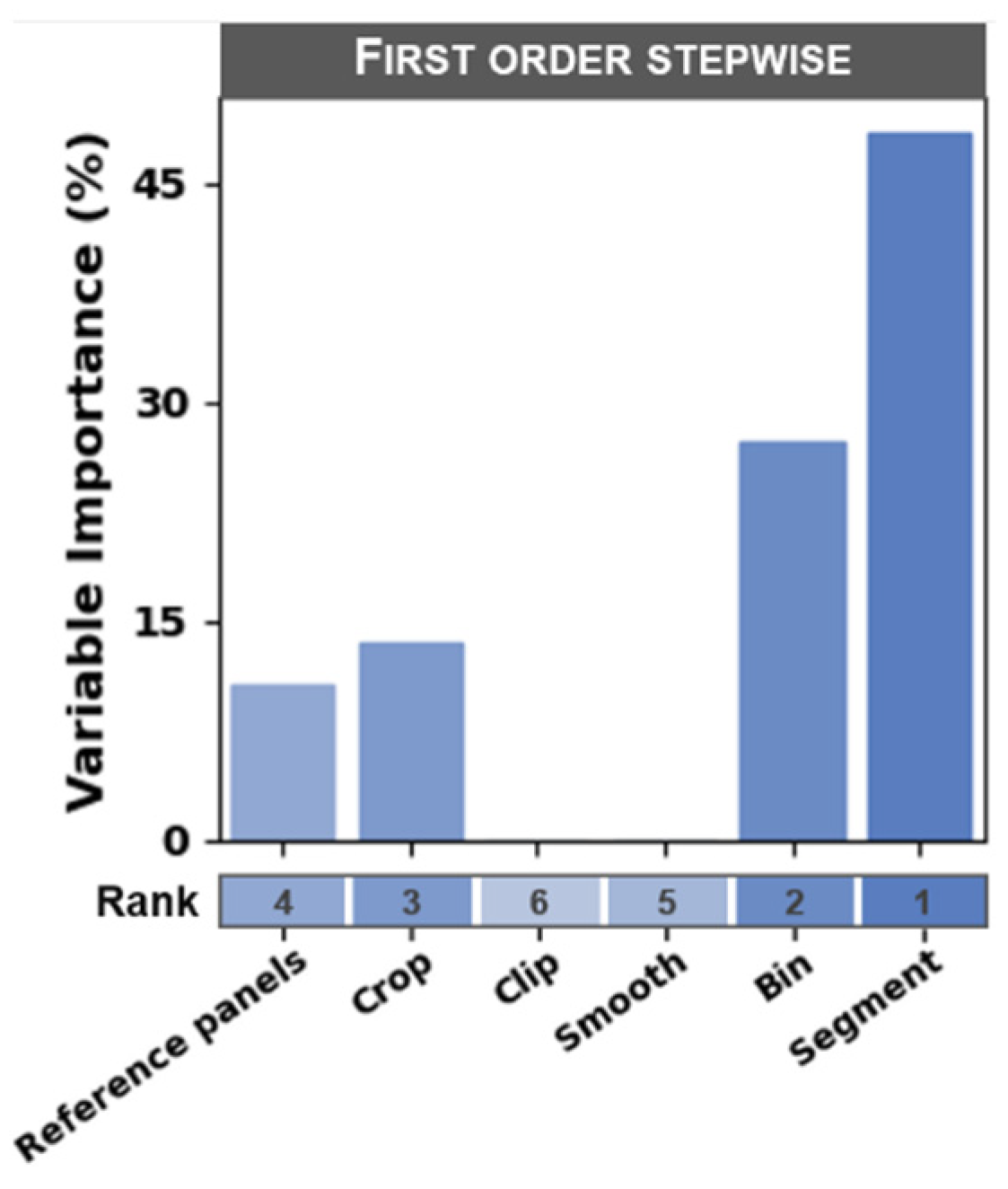
3.3. Ranking of Processing Steps by Influence on Model Error

The purpose of both the sensitivity analysis and forward-selection stepwise regression analysis was to identify the processing steps that had the greatest influence on estimator error across all workflow scenarios. The segment and bin processing steps had the greatest influence on estimator error, whereas the clip and smooth steps had the least influence (rankings are presented in Figure 5). The forward-selection stepwise regression approach resulted in variable importance rankings that were similar to the sensitivity analysis rankings (Figure 6). The only minor exception to these ranks was that the ranking between the crop and reference panels steps were swapped for first-order sensitivity calculated according to the Sobol method (i.e., the reference panels step was ranked as the third most sensitive step and the crop step was ranked as the fourth most sensitive step). Each processing step resulted in a total-order sensitivity index greater than its corresponding first-order sensitivity index, indicating that there were substantial interactions in model error among the processing steps.

3.4. Cumulative Error at Each Processing Step

The empirical cumulative density function (ECDF) for each processing scenario was plotted to quantify and effectively compare the model RMSE that resulted at each processing step (Figure 7). The ECDF is helpful for interpreting these results because it illustrates the proportion of workflow scenarios represented by a given error threshold for each scenario. Please note that a lower RMSE indicates a better model fit and is generally more desirable than a higher RMSE is.

Figure 7 is rich in information, but the ECDF plots reveal three key characteristics that help to evaluate the suitability of each image processing scenario. Each of these characteristics is highlighted in Figure 8. Please note that these characteristics do not necessarily manifest at each processing step. The three processing steps used in Figure 8 (i.e., reference panels, crop, and segment) were adapted from Figure 7 and are used only as examples to highlight the key characteristics. They do not imply the characteristics are exclusive to these processing steps.

The first characteristic of the ECDF plots is the clear indication of the likelihood for achieving a defined error threshold (Figure 8a). If the analyst defines their error threshold for a particular business solution as <15 kg ha⁻¹, they can easily infer the likelihood of satisfying this requirement. Using the reference panels step as an example (Figure 8a), observe that it was much more likely that the all panels scenario resulted in an RMSE less than 15 kg ha⁻¹ than did the closest panel scenario. In fact, as indicated by the grid above the ECDF plot, 16% of all workflow scenarios that used the all panels scenario had an RMSE < 15 kg ha⁻¹, while only 2.0% of all workflow scenarios that used the closest panel scenario had an RMSE in that same threshold range. Thus, if a particular business solution requires an RMSE less than 15 kg ha⁻¹ for this particular dataset/objective, the analyst can infer they are much more likely to achieve a result that satisfies their requirement by choosing to use the all panels rather than the closest panel processing approach. There is some uncertainty in the ECDF plots that can be revealed via bootstrapping (not presented). Logistic regression can be used to achieve a statistically reliable comparison of the difference among scenarios at a particular RMSE threshold. This analysis showed that the clip step was the only processing step in this study that did not produce statistically different likelihoods among scenarios below the 15 kg ha⁻¹ RMSE threshold (α = 0.001; p = 0.65 for the clip step).

Shifting the focus to the clip step (which was much less sensitive than the reference panels step), observe that there is little difference among the three clip scenarios (Figure 7). Specifically, 8.3%, 9.7%, and 9.0% of workflow scenarios fall within the 14 kg ha⁻¹ < RMSE < 15 kg ha⁻¹ threshold for the no spectral clipping, ends clipped, and ends + H₂O and O₂ absorption scenarios, respectively. Thus, the analyst may be 16% more likely to achieve their desired result by choosing the ends clipped scenario instead of the no spectral clipping scenario. However, the decision about how to perform the clip step is not nearly as crucial as the decision about how to perform the reference panels step if only considering the likelihood of achieving a defined error threshold (Figure 8a).

The second characteristic is the ability to evaluate processing scenarios by their upside (i.e., potential for low RMSE values) and downside (potential for high RMSE values; Figure 8b). With all other characteristics equal, the analyst should generally be looking for the workflow scenario(s) with greater upside and lesser downside. As highlighted in Figure 8b for the crop step, the by plot boundary scenario had a much greater downside than the edges cropped scenario did. In this example, the potential error was close to 20 kg ha⁻¹ for the by plot boundary scenario, but less than 18 kg ha⁻¹ for the edges cropped scenario. The upside between scenarios was relatively similar, but the edges cropped scenario had a lesser downside. This indicates that the edges cropped scenario must have had a lower RMSE across most workflow scenarios.

The third characteristic revealed by the ECDF plots is the error stability for each processing scenario (Figure 8c). Error stability can be interpreted as the consistency in RMSE values across workflow scenarios and is inversely related to the range in RMSE values (i.e., a narrow range indicates greater error stability). With all other characteristics equal, greater error stability is more desirable. Consider the ECDF of the no segmenting and NDVI > 50th scenarios in the segment step (Figure 8c). At low RMSE values, the no segmenting scenario represented a relatively higher proportion of workflow scenarios than the NDVI > 50th scenario did, but then as the RMSE approached ~16 kg ha⁻¹, the ECDF plots crossed one another and the NDVI > 50th scenario began to represent a relatively higher proportion of workflow scenarios. Thus, because the NDVI > 50th scenario had a greater range in RMSE values across workflow scenarios, it was more stable than the no segmenting scenario.

The relative value of these characteristics may vary depending on the processing step, use case, dataset, or business need being evaluated. This is demonstrated with two examples. First, recall the similar upsides at the crop step (Figure 8b). Alone, knowing that upsides were similar does not help to choose which scenario is more desirable. However, when considering the first characteristic pointed out in Figure 8a, we observe that the likelihood of achieving an RMSE value less than 15–16 kg ha⁻¹ was much greater if the edges cropped scenario was chosen. Second, recall that the ECDF plots crossed one another at the segment step (Figure 8c). Although the NDVI > 50th scenario was more stable (which is generally more desirable), it had a lesser upside (which is generally less desirable). In this case (ignoring all other segment scenarios for the time being), the analyst must weigh the benefits of error stability against the possibility of a higher upside.

It was useful to examine the processing steps in Figure 7 to identify the scenarios that demonstrated any of the key characteristics mentioned in Figure 8. At the smooth step, the upsides and downsides of each scenario were similar, but the Savitzky–Golay smoothing scenario demonstrated a higher distribution within the 14 kg ha⁻¹ < RMSE < 15 kg ha⁻¹ NUP range. At the bin step, the no spectral binning and spectral “bin”—20 nm scenarios were roughly similar, while the spectral “mimic”—Sentinel-2A scenario had both a lesser upside and a greater downside, indicating a loss of signal with the Sentinel-2A band configuration. While the Sentinel-2A band configuration did not perform as well, it is perhaps more practical for many analysts to deploy models that can be deployed broadly with multispectral imagery rather than models that use specialized hyperspectral imagery.

The segment step was perhaps the most interesting of all steps evaluated because of the diverse ECDF plots for each of its scenarios. To help interpret the results of the nine segment scenarios, they were grouped based on the similarity of their upside and downside characteristics (

Table 3. Minimum, maximum, and range of nitrogen uptake root mean squared error (RMSE) for each of the processing scenarios at the segment step. The scenarios are grouped by their relative upside (greater potential for low error) and downside (greater potential for high error) characteristics. Stability (range) refers to the consistency in RMSE values (across workflow scenarios).

	--------RMSE (kg ha−1)---------
Segment Scenario	Upside (Minimum)	Downside (Maximum)	Stability (Range)
High upside; low downside	(consistently good)
MCARI2 > 50th	14.3 1	16.4	2.1
50th > MCARI2 < 75th	14.4	16.7	2.3
75th > MCARI2 < 95th	14.4	17.0	2.6
High upside; high downside	(variable)
No segmenting	14.6	17.4	2.8
MCARI2 > 90th	14.6	17.6	3.0
MCARI2 > 90th; green > 75th	14.3 2	17.9	3.6
Low upside; low downside	(consistently mediocre)
NDVI > 50th	14.8	16.7	1.8
Low upside; high downside	(consistently poor)
NDVI < 50th	14.9	19.2	4.3
MCARI2 < 50th	15.2	19.8	4.6
All scenarios	14.3	19.8	5.5

¹ Rounded to the nearest thousandth: 14.311 kg ha⁻¹, ² Rounded to the nearest thousandth: 14.309 kg ha^−1.

). Scenarios with a high upside and low downside (e.g., MCARI2 > 50th, 50th > MCARI2 < 75th, and 75th > MCARI2 < 95th) were most ideal because error results were consistently good, whereas scenarios with low upside and high downside (e.g., NDVI < 50th and MCARI2 < 50th) were least ideal because error results were consistently poor. Scenarios with high upside and high downside (e.g., No segmenting, MCARI2 > 90th, and MCARI2 > 90th; green > 75th) demonstrated greater variability in error results. Because they had a relatively high risk of poor results, they are less ideal than other segmentation scenarios. The NDVI > 50th scenario had the lowest RMSE range of all segment scenarios, indicating more stable error results across workflow scenarios from the other five processing steps. It was considered consistently mediocre, however, because of the low upside.

3.5. Comparing the Processing Workflow of a Previous Study

Across all workflow scenarios, the RMSE ranged from 14.3 to 19.8 kg ha⁻¹ (relative RMSE ranged from 26.5% to 36.5%), a 38.5% increase in error between the lowest and highest error workflow scenarios (

Table 4. The image processing workflow with the lowest and highest root mean squared error (RMSE), as well as the processing workflow chosen by Nigon et al. (2020). The error, the percent increase in error compared to the workflow with the lowest error, and the corresponding percentile across all unique scenarios evaluated in this study are listed for each of the three scenarios.

		Lowest Error	Highest Error	Nigon et al. (2020) [20]
Processing step
1	Reference panels	All panels	All panels	Closest panel
2	Crop	Edges cropped	By plot boundary	By plot boundary
3	Clip	No spectral clipping	Ends + H2O and O2 absorption	Ends + H2O and O2 absorption
4	Smooth	Savitzky–Golay smoothing	Savitzky–Golay smoothing	Savitzky–Golay smoothing
5	Bin	No spectral binning	Spectral “mimic”-Sentinel-2A	No spectral binning
6	Segment	MCARI2 > 90th; green > 75th	MCARI2 < 50th	MCARI2 > 90th
RMSE (kg ha−1)		14.3 (+0.0%)	19.8 (+38.5%)	16.5 (+15.4%)
Percentile		0.309	99.9	71.5

). Table 4 lists the scenarios used at each processing step for both the lowest and highest error workflow scenarios. It may be interesting to note that the same processing scenarios were used at the reference panels (i.e., all panels) and smoothing (i.e., Savitzky–Golay smoothing) steps for both the lowest and highest error scenarios, indicating there are interactions at play among the processing steps.

The processing workflow used by [20] is listed in Table 4 to contrast the lowest and highest error workflow scenarios with that of a subjective choice (i.e., the subjectivity being the authors training, experience, and other expert knowledge rather than a data-driven choice). Between [20] and the lowest error workflow scenario, only two of the six processing steps were similar: the smooth (Savitzky–Golay smoothing) and bin steps (no spectral binning). The workflow scenario used by [20] had an RMSE of 16.5 kg ha⁻¹, a 15.4% increase in error compared with choosing the workflow scenario with the lowest error. Across all workflow scenarios evaluated, the corresponding RMSE percentile of the scenario chosen by [20] was 71.5, which indicates that their choice in image processing had a lower error than only 28.5% of the scenarios evaluated.

4. Discussion

4.1. Practical Insights for the Use Case Evaluated in this Study

Recall that the primary goals of image processing are to improve the signal and to improve the consistency of image data in order to achieve a particular objective or business solution. There are many possible image processing steps and scenarios that can be performed. Ultimately, the method selected should be based on the use case and research objectives [6]. This study used high-resolution hyperspectral aerial imagery to predict nitrogen uptake in maize, so we focused attention on the relevant processing steps within this context. The processing steps used in this study were not an exhaustive list of possible image processing steps, nor were the scenarios explored within each step. Our discussion will focus on the implications of the findings and how they are helpful from a practical perspective in the context of tradeoffs already discussed in the Materials and Methods (Section 2.5).

4.1.1. Reference Panels

Inconsistent radiance values among images captured in the same flight can originate from differences in local viewing and illumination geometry for each image pixel [53]. At the reference panels step, results suggested that dampening inconsistent radiance values among images captured in the same flight (i.e., effect of the all panels scenario) performed better than adjusting for illumination inconsistencies throughout image acquisition (effect of the closest panel scenario) did. The results provide guidance to future studies that require a similar experimental design with relatively uniform illumination (within an individual flight) and field topography. Although this was the case for this use case and this dataset, keep in mind that datasets collected under different illumination conditions and different topography may show different results.

4.1.2. Crop

Cropping by the effective ground truth sampling area (i.e., edges cropped scenario) consistently performed better than cropping by plot boundary did, but the processing scenario requires attention to detail regarding which row(s) and plants were sampled at each date. Given that the absolute accuracy from the georectification step was only ~3–4 m for the images used in this study and that many plots were similar in size (Table A1), additional efforts were required to improve absolute georectification accuracy while cropping the images (i.e., ground targets were placed in plot corners to help identify true plot corners from aerial images). The spatial_mod class of the HS-Process Python package [37] provides some useful functions for streamlining the cropping procedure, but only after identifying the corner pixel coordinates of at least one plot in each image. Although these additional efforts provided a consistently positive outcome for the use case explored in this study, it may be more effort than some analysts would like to exert. Performing “precision cropping” (i.e., edges cropped scenario) may not be possible without adequate pixel resolution.

4.1.3. Clip and Smooth

The clip and smooth steps had very little influence on model error as indicated by the sensitivity analysis. The effects of clipping during image processing were probably negated by the effects of feature selection during model training because clipping and feature selection have the same impacts on data considered by the estimator. There was no apparent negative consequence to model error when data were smoothed via Savitzky–Golay smoothing. Although smoothing was not all that sensitive, there were improved model outcomes for the lowest error/highest performance workflow scenarios.

4.1.4. Bin

The decision to bin spectral data may be considered for a couple of reasons. First, binning data is a reasonable method to reduce the feature number, which may be a desirable way to simplify the trained model during analysis. Hyperspectral data are mostly redundant on the spectral domain (especially if smoothing was performed), and binning those redundant parts of the spectrum can substantially reduce data size without necessarily compromising the informative value. Second, binning hyperspectral data based on the radiometric specifications of another sensor may create substantial practical value in the scale at which a trained estimator can be deployed. For example, hyperspectral data can be collected with ground truth measurements to serve as a historical dataset that can be molded into numerous multispectral datasets similar to the spectral “mimic”—Sentinel-2A scenario evaluated in this study. Using hyperspectral data as the input, this mimicking procedure can be achieved for the radiometric specification of any sensor if the spectral response of the sensor is available (with satisfactory spectral precision) and the relevant spectral bands/range of wavelengths are represented.

The main consideration at the bin step is weighing the increased error against the potential added value of broader model deployment. In other words, it is important to understand if the increased error that resulted from mimicking the Sentinel-2A spectral configuration is tolerable if the benefit is that the model can be deployed across larger areas or at cheaper costs. Deploying a model that is slightly suboptimal may mean that a more practical sensor, platform, etc. could be used to collect new data on which to make predictions. Practicality could be measured in many ways depending on individual practitioners needs, such as ease of use, time from acquisition to analysis, cost, and popularity/acceptance.

4.1.5. Segment

Because the segmentation step had the most influence on model error among all other processing steps, optimization efforts are critical. The segmentation analysis showed that it can do just as much harm as good. Because of the virtually infinite segmentation possibilities with high-resolution hyperspectral imagery, there is a lot of potential to discover novel segmentation scenarios and improve model performance further. The advantage of the framework presented here is that the data-driven methodology produces the optimum solution for the use case. This study only considered three spectral layers (i.e., NDVI, MCARI2, and green reflectance) for segmentation, but there are hundreds of spectral indices that may be worthwhile considering depending on the use case. The thresholds used to mask out unwanted pixels are also important. While arbitrary, the thresholds in this study were chosen to get a variety of intervals from the spectral layers to understand the overall sensitivity of the segmentation step. A more thorough analysis of segmentation thresholds for different spectral layers may reveal some interesting characteristics around which pixels contribute the most meaningful information for model training. Finally, segmentation in multiple steps can be important to add auxiliary features that improve the informative value of the feature set available for model training [20].

4.2. Choosing an Image Processing Workflow

While choosing the optimal processing workflow that resulted in the least error (Table 4) may be sufficient for specific research objective/business need, caution must be exercised if results show one or more of the processing scenarios in the optimal workflow are unstable. In this study, the MCARI2 > 90th; green > 75th scenario was the optimal scenario at the segment step (Table 4), but the MCARI2 > 90th; green > 75th scenario was unstable compared to other scenarios at the segment step (Figure 7; Table 3). This raises an important point: the analyst’s level of risk aversion may influence what is considered the most suitable processing scenario. It is also worth noting that the MCARI2 > 90th; green > 75th and MCARI2 > 50th scenarios had virtually the same RMSEs: 14.309 and 14.311 kg ha⁻¹, respectively (i.e., within two thousandths kg ha⁻¹ or 0.01% of each other; Table 3). The MCARI2 > 90th; green > 75th scenario was technically the optimal scenario, but it practically had little difference to the MCARI2 > 90th scenario and was also less stable than the MCARI2 > 90th scenario was.

The results from this study demonstrate there are interactions across processing steps that require further analysis to adequately understand their implications. To help improve understanding of the interactions and to help weigh the tradeoffs of processing scenarios, three key characteristics were described (Figure 8). In addition, Table 3 introduced a method for grouping the scenarios at the segment step based on two of these key characteristics: upside versus downside and error stability. The three key characteristics from ECDF plots should apply broadly across different use cases and for different image processing steps and scenarios.

4.3. Benefits of Integrating Image Processing and Model Training

The range of experimental conditions to create a biophysical prediction model (e.g., sensors, platforms, ground-truth variables, and environments) is virtually infinite, which makes it nearly impossible to objectively compare the methods used in two different studies [16]. Building a streamlined processing and model-training framework required substantial effort, but it allowed us to identify the processing steps that had the greatest influence on prediction error, and it allowed us to quantify the influence of 648 unique processing workflow scenarios on prediction error. Ultimately, the streamlined processing and model-training framework was used to optimize the image processing workflow based on prediction error. Results from the use case demonstrated that error was improved substantially through this optimization process compared to the processing workflow used by [20]. A key takeaway from the comparison with [20] was that although they used an acceptable image processing protocol based on their training, experience, and other expert knowledge, their subjective choice in processing workflow resulted in a higher RMSE than over 70% of the 648 workflow scenarios evaluated. Odds are that performance would have been improved if the choice of image processing workflow was instead randomly chosen from the 648 workflow scenarios evaluated in this study.

The lack of consistent benchmarks for evaluating image processing and analysis protocol under real-world conditions has been recognized in the remote sensing community [16]. The insights provided via the framework brought forward in this study do not set explicit benchmarks per se. That was not necessarily the motivation for this work. Instead, this framework provides a general methodology that allows remote sensing analysts to both improve model performance and improve the reproducibility and objectivity of their research and development efforts—the two major benefits of hyperparameter optimization in the automated machine learning discipline [18,19].

The framework allows analysts to provide a results-driven justification for their image processing workflow. It provides some level of satisfaction to those analysts that find themselves asking (i) when a satisfactory level of image processing has been reached, (ii) which image processing steps are most important, or (iii) how a particular processing step should be implemented for a use case. Because the range of experimental conditions to create a biophysical prediction model (e.g., sensors, platforms, ground-truth variables, and environments) is virtually infinite, it is nearly impossible to objectively compare the methods used in two different studies [16]. It relaxes the idea that explicit benchmarks or datasets are needed, and instead embraces the nuances and complexity of image processing on model performance, similar to hyperparameter optimization in the automated machine learning discipline. It enables analysts to determine which processing steps are most sensitive to the model being trained and allows them to focus their attention/efforts there. It embraces the data-dependency issue [6,17] by optimizing the image processing workflow regardless of the sensors, platforms, experimental conditions, etc. being implemented.

Statistical optimization techniques are being recognized for their importance towards the increased adoption of precision agriculture technologies [54], in part because of the advantages they offer in handling the specificity and high-dimensional nature of big data in agriculture. This dimensionality problem is only being exacerbated with advanced sensor technologies such as hyperspectral imagery [5], highlighting the need for robust, straightforward protocols aimed at delivering optimized machine learning models.

4.4. Software and Computation Requirements

Python was an ideal programming language to implement this framework because the availability of robust geospatial libraries (i.e., GDAL, Geopandas, HS-Process, and Spectral Python) allowed for customization of the image processing steps and workflow scenarios. The script was designed so that the image processing steps and workflow scenarios could be configured/parameterized at a high level via a single control file. Having the control file was convenient because the order of processing steps and the scenarios to be evaluated at each step could be modified. Upon modification, all image processing tasks were performed for all images/observations by simply running the script. This is noteworthy because it was generally very easy to reprocess imagery after reordering, adding, or modifying any processing steps/scenarios. Adjustments made at early processing steps after imagery was already processed once did not mean that substantial additional efforts had to be made to reprocess the entire image dataset (only additional compute resources and time were necessary). Even with batch processing, image processing tends to be tedious and monotonous, in part because of the large data size and subtle variations among experimental datasets (i.e., pixel size and plot size/observation area may necessitate slight differences in how images are processed). Scripting out image processing steps, with complete flexibility in the configuration/parameterization via a control file, greatly reduced the tedious and monotonous nature of image processing.

Although we intended to entirely automate the image processing workflow and carry out the subsequent model training in the same workflow, the framework was not entirely automated. The first three image processing steps (i.e., radiance conversion, georectification, and reflectance conversion) were implemented in Spectronon (Figure 1), mostly using their batch-processing utilities. Spectronon was used because it closely integrates with Resonon hyperspectral imagery and because it could perform these first three processing steps in a straightforward way. The workflow would have required substantially more effort than what was already necessary if these three steps could not be performed first. We would have likely had to remove the dependency on Spectronon by finding Python libraries that could satisfactorily replace the relevant capabilities of Spectronon. Another option may have been to write custom Spectronon plugins or scripts to perform each of the necessary workflow tasks from the Spectronon environment, but this was not practical for this stage of research.

There are many excellent image processing software solutions available to remote sensing analysts [5], including ENVI (Exelis Visual Information Solutions, Boulder, CO, USA) and PARGE (ReSe Applications Schläpfer, Wil, Switzerland) [5], and a growing number of image processing capabilities in programming languages such as Python, R, or Matlab. However, realistically implementing the framework described in this study is only practical if the software has four fundamental capabilities. First, the software must have the ability to perform any image processing step and be customizable to any number of scenarios to satisfy the interests of the analyst. Second, the software must have the ability to manage multiple (potentially hundreds or thousands) image processing workflow scenarios. Third, the software must have the ability to perform model training and cross-validation in a way that traces the image processing parameters and summarizes the error/accuracy results for each workflow scenario. Finally, the software must have the ability to run on high-performance compute (e.g., parallelization) and storage resources that can process imagery efficiently and handle large datasets. The use case in this study, which had 407 hyperspectral image observations, created ~10 TB of data across the 648 image processing scenarios.

5. Conclusions

A use case with aerial hyperspectral imagery to predict early season maize nitrogen uptake was used to demonstrate the benefits of optimizing the image processing workflow. Results derived from this framework allow remote sensing analysts to improve model performance while providing data-driven justification to improve the reproducibility and objectivity of their work. The framework embraces the nuances and complexity of image processing on model performance, similar to hyperparameter optimization in the automated machine learning discipline. Model adjustments and performance were improved by knowing which processing steps were most sensitive to estimator error. Optimizing the image processing workflow embraces data-dependency and shifts the focus to optimal model performance for the individual dataset or problem of interest. Although the processing workflow that minimized error was successfully determined, choosing the most suitable image processing workflow may not be quite that simple. Other key characteristics revealed by ECDF plots may be important to consider as well, particularly consideration of upside versus downside or error stability of a particular processing scenario relative to other scenarios. Remote sensing analysists may ultimately consider their aversion to risk in addition to the most optimal processing scenario(s) when choosing the most suitable workflow for their problem.

The framework and characteristics introduced in this study should be applicable to train other supervised and unsupervised prediction models using aerial imagery that requires some level of image processing. We believe it can be implemented across a broad array of remote sensing machine learning problems. Different experimental objectives or business needs require different types of machine learning models (e.g., change detection, classification, clustering, or regression) and tasks (i.e., unsupervised and supervised). Future research should evaluate the framework for these different approaches, as well as for other sensors, platforms, and experimental objectives. Specifically, we should understand the similarities and differences of the framework across the seemingly infinite number of possible use cases. If the remote sensing community generally finds value in optimization of the image processing workflow (i.e., for many different use cases), then efforts should be invested in developing more automated, easy-to-use software solutions that integrate with existing remote sensing software.

References

1. Aasen, H.; Burkart, A.; Bolten, A.; Bareth, G. Generating 3D hyperspectral information with lightweight UAV snapshot cameras for vegetation monitoring: From camera calibration to quality assurance. ISPRS J. Photogramm. Remote Sens. 2015, 108, 245–259. [Google Scholar] [CrossRef]
2. Adão, T.; Hruška, J.; Pádua, L.; Bessa, J.; Peres, E.; Morais, R.; Sousa, J. Hyperspectral Imaging: A Review on UAV-Based Sensors, Data Processing and Applications for Agriculture and Forestry. Remote Sens. 2017, 9, 1110. [Google Scholar] [CrossRef] [Green Version]
3. Honkavaara, E.; Saari, H.; Kaivosoja, J.; Pölönen, I.; Hakala, T.; Litkey, P.; Mäkynen, J.; Pesonen, L. Processing and Assessment of Spectrometric, Stereoscopic Imagery Collected Using a Lightweight UAV Spectral Camera for Precision Agriculture. Remote Sens. 2013, 5, 5006–5039. [Google Scholar] [CrossRef] [Green Version]
4. Jakob, S.; Zimmermann, R.; Gloaguen, R. The Need for Accurate Geometric and Radiometric Corrections of Drone-Borne Hyperspectral Data for Mineral Exploration: MEPHySTo—A Toolbox for Pre-Processing Drone-Borne Hyperspectral Data. Remote Sens. 2017, 9, 88. [Google Scholar] [CrossRef] [Green Version]
5. Lu, B.; Dao, P.; Liu, J.; He, Y.; Shang, J. Recent Advances of Hyperspectral Imaging Technology and Applications in Agriculture. Remote Sens. 2020, 12, 2659. [Google Scholar] [CrossRef]
6. Jia, B.; Wang, W.; Ni, X.; Lawrence, K.C.; Zhuang, H.; Yoon, S.-C.; Gao, Z. Essential processing methods of hyperspectral images of agricultural and food products. Chemom. Intell. Lab. Syst. 2020, 198, 103936. [Google Scholar] [CrossRef]
7. Duan, S.-B.; Li, Z.-L.; Tang, B.-H.; Wu, H.; Ma, L.; Zhao, E.; Li, C. Land Surface Reflectance Retrieval from Hyperspectral Data Collected by an Unmanned Aerial Vehicle over the Baotou Test Site. PLoS ONE 2013, 8, e66972. [Google Scholar] [CrossRef]
8. Tan, K.; Niu, C.; Jia, X.; Ou, D.; Chen, Y.; Lei, S. Complete and accurate data correction for seamless mosaicking of airborne hyperspectral images: A case study at a mining site in Inner Mongolia, China. ISPRS J. Photogramm. Remote Sens. 2020, 165, 1–15. [Google Scholar] [CrossRef]
9. Arroyo-Mora, J.P.; Kalacska, M.; Løke, T.; Schläpfer, D.; Coops, N.C.; Lucanus, O.; Leblanc, G. Assessing the impact of illumination on UAV pushbroom hyperspectral imagery collected under various cloud cover conditions. Remote Sens. Environ. 2021, 258, 112396. [Google Scholar] [CrossRef]
10. Olsson, P.-O.; Vivekar, A.; Adler, K.; Garcia Millan, V.E.; Koc, A.; Alamrani, M.; Eklundh, L. Radiometric Correction of Multispectral UAS Images: Evaluating the Accuracy of the Parrot Sequoia Camera and Sunshine Sensor. Remote Sens. 2021, 13, 577. [Google Scholar] [CrossRef]
11. Poncet, A.M.; Knappenberger, T.; Brodbeck, C.; Fogle, M.; Shaw, J.N.; Ortiz, B.V. Multispectral UAS Data Accuracy for Different Radiometric Calibration Methods. Remote Sens. 2019, 11, 1917. [Google Scholar] [CrossRef] [Green Version]
12. Cao, J.; Leng, W.; Liu, K.; Liu, L.; He, Z.; Zhu, Y. Object-Based Mangrove Species Classification Using Unmanned Aerial Vehicle Hyperspectral Images and Digital Surface Models. Remote Sens. 2018, 10, 89. [Google Scholar] [CrossRef] [Green Version]
13. Cheng, J.; Bo, Y.; Zhu, Y.; Ji, X. A novel method for assessing the segmentation quality of high-spatial resolution remote-sensing images. Int. J. Remote Sens. 2014, 35, 3816–3839. [Google Scholar] [CrossRef]
14. Zhang, C.; Jiang, W.; Zhao, Q. Semantic Segmentation of Aerial Imagery via Split-Attention Networks with Disentangled Nonlocal and Edge Supervision. Remote. Sens. 2021, 13, 1176. [Google Scholar] [CrossRef]
15. Saldana Ochoa, K.; Guo, Z. A framework for the management of agricultural resources with automated aerial imagery detection. Comput. Electron. Agric. 2019, 162, 53–69. [Google Scholar] [CrossRef]
16. Gewali, U.B.; Monteiro, S.T.; Saber, E. Machine learning based hyperspectral image analysis: A survey. arXiv 2018, arXiv:1802.08701. [Google Scholar]
17. Masi, G. Image Segmentation in a Remote Sensing Perspective; University of Naples Federico II: Naples NA, Italy, 2016. [Google Scholar]
18. Feurer, M.; Hutter, F. Hyperparameter Optimization. In Studies in Computational Intelligence; Hutter, F., Kotthoff, L., Vanschoren, J., Eds.; The Springer Series on Challenges in Machine Learning; Springer International Publishing: Cham, Switzerland, 2019; Volume 498, pp. 3–33. ISBN 978-3-030-05317-8. [Google Scholar]
19. Snoek, J.; Larochelle, H.; Adams, R.P. Practical Bayesian optimization of machine learning algorithms. Adv. Neural Inf. Process. Syst. 2012, 4, 2951–2959. [Google Scholar]
20. Nigon, T.J.; Yang, C.; Dias Paiao, G.; Mulla, D.J.; Knight, J.F.; Fernández, F.G. Prediction of Early Season Nitrogen Uptake in Maize Using High-Resolution Aerial Hyperspectral Imagery. Remote Sens. 2020, 12, 1234. [Google Scholar] [CrossRef] [Green Version]
21. Earth Observation and Research Branch Team. Crop Identification and BBCH Staging Manual: SMAP-12 Field Campaign; Agriculture and Agri-Food Canada: Ottawa, ON, Canada, 2011; pp. 1–50. Available online: https://smapvex12.espaceweb.usherbrooke.ca/BBCH_STAGING_MANUAL_GENERAL_ALL_CROPS.pdf (accessed on 28 October 2021).
22. Kaiser, D.E.; Lamb, J.A.; Eliason, R. Fertilizer Guidelines for Agronomic Crops in Minnesota; University of Minnesota Extension: Saint Paul, MN, USA, 2011; Available online: https://conservancy.umn.edu/bitstream/handle/11299/198924/Fertilizer%20Guidelines%20for%20Agronomic%20Crops%20in%20Minnesota.pdf?sequence=1&isAllowed=y (accessed on 28 October 2021).
23. Jones, J.B., Jr.; Case, V.W. Sampling, Handling, and Analyzing Plant Tissue Samples. In Soil Testing and Plant Analysis; Westerman, R.L., Ed.; SSSA Book Series; Soil Science Society of America: Madison, WI, USA, 1990; pp. 389–427. ISBN 9780891188629. [Google Scholar]
24. Bradstreet, R.B. Kjeldahl Method for Organic Nitrogen. Anal. Chem. 1954, 26, 185–187. [Google Scholar] [CrossRef]
25. Matejovic, I. Total nitrogen in plant material determinated by means of dry combustion: A possible alternative to determination by kjeldahl digestion. Commun. Soil Sci. Plant Anal. 1995, 26, 2217–2229. [Google Scholar] [CrossRef]
26. Smith, G.M.; Milton, E.J. The use of the empirical line method to calibrate remotely sensed data to reflectance. Int. J. Remote Sens. 1999, 20, 2653–2662. [Google Scholar] [CrossRef]
27. Richter, R.; Schlapfer, D.; Muller, A. Operational Atmospheric Correction for Imaging Spectrometers Accounting for the Smile Effect. IEEE Trans. Geosci. Remote Sens. 2011, 49, 1772–1780. [Google Scholar] [CrossRef]
28. Greenblatt, G.D.; Orlando, J.J.; Burkholder, J.B.; Ravishankara, A.R. Absorption measurements of oxygen between 330 and 1140 nm. J. Geophys. Res. 1990, 95, 18577. [Google Scholar] [CrossRef] [Green Version]
29. Hill, C.; Jones, R.L. Absorption of solar radiation by water vapor in clear and cloudy skies: Implications for anomalous absorption. J. Geophys. Res. Atmos. 2000, 105, 9421–9428. [Google Scholar] [CrossRef]
30. Press, W.H.; Teukolsky, S.A. Savitzky-Golay Smoothing Filters. Comput. Phys. 1990, 4, 669. [Google Scholar] [CrossRef]
31. Ravikanth, L.; Jayas, D.S.; White, N.D.G.; Fields, P.G.; Sun, D.-W. Extraction of Spectral Information from Hyperspectral Data and Application of Hyperspectral Imaging for Food and Agricultural Products. Food Bioprocess Technol. 2017, 10, 1–33. [Google Scholar] [CrossRef]
32. Savitzky, A.; Golay, M.J.E. Smoothing and Differentiation of Data by Simplified Least Squares Procedures. Anal. Chem. 1964, 36, 1627–1639. [Google Scholar] [CrossRef]
33. Space Agency, E. Sentinel-2 Spectral Response Functions. Available online: https://dragon3.esa.int/web/sentinel/technical-guides/sentinel-2-msi/performance (accessed on 29 January 2021).
34. Rouse, J.W.; Haas, R.H.; Schell, J.A.; Deering, D.W. Monitoring Vegetation Systems in the Great Plains with ERTS; NASA: Washington, DC, USA, 1974; Volume 1, pp. 309–317.
35. Huete, A. A soil-adjusted vegetation index (SAVI). Remote Sens. Environ. 1988, 25, 295–309. [Google Scholar] [CrossRef]
36. Haboudane, D.; Miller, J.R.; Pattey, E.; ZarcoTejada, P.J.; Strachan, I.B. Hyperspectral vegetation indices and novel algorithms for predicting green LAI of crop canopies: Modeling and validation in the context of precision agriculture. Remote Sens. Environ. 2004, 90, 337–352. [Google Scholar] [CrossRef]
37. Nigon, T.J. HS-Process 2020. Available online: https://hs-process.readthedocs.io/ (accessed on 28 October 2021).
38. Boggs, T. Spectral Python 2019. Available online: https://www.spectralpython.net/ (accessed on 28 October 2021).
39. GDAL/OGR Geospatial Data Abstraction Library. Available online: https://gdal.org/ (accessed on 28 October 2021).
40. Nigon, T.J. SIP. 2021. Available online: https://github.com/tnigon/sip/ (accessed on 28 October 2021).
41. Yeo, I.-K.; Johnson, R.A. A new family of power transformations to improve normality or symmetry. Biometrika 2000, 87, 954–959. [Google Scholar] [CrossRef]
42. Tibshirani, R. Regression shrinkage and selection via the Lasso. J. R. Stat. Soc. Ser. B 1996, 58, 267–288. [Google Scholar] [CrossRef]
43. Cukier, R.I.; Fortuin, C.M.; Shuler, K.E.; Petschek, A.G.; Schaibly, J.H. Study of the sensitivity of coupled reaction systems to uncertainties in rate coefficients. I Theory. J. Chem. Phys. 1973, 59, 3873–3878. [Google Scholar] [CrossRef]
44. Saltelli, A.; Tarantola, S.; Chan, K.P.-S. A Quantitative Model-Independent Method for Global Sensitivity Analysis of Model Output. Technometrics 1999, 41, 39–56. [Google Scholar] [CrossRef]
45. Sobol, I.M. Global sensitivity indices for nonlinear mathematical models and their Monte Carlo estimates. Math. Comput. Simul. 2001, 55, 271–280. [Google Scholar] [CrossRef]
46. Saltelli, A.; Annoni, P.; Azzini, I.; Campolongo, F.; Ratto, M.; Tarantola, S. Variance based sensitivity analysis of model output. Design and estimator for the total sensitivity index. Comput. Phys. Commun. 2010, 181, 259–270. [Google Scholar] [CrossRef]
47. Saltelli, A. Making best use of model evaluations to compute sensitivity indices. Comput. Phys. Commun. 2002, 145, 280–297. [Google Scholar] [CrossRef]
48. Zhang, X.; Trame, M.; Lesko, L.; Schmidt, S. Sobol Sensitivity Analysis: A Tool to Guide the Development and Evaluation of Systems Pharmacology Models. CPT Pharmacomet. Syst. Pharmacol. 2015, 4, 69–79. [Google Scholar] [CrossRef]
49. Waskom, M. Seaborn: Statistical data visualization. J. Open Source Softw. 2021, 6, 3021. [Google Scholar] [CrossRef]
50. Sturges, H.A. The Choice of a Class Interval. J. Am. Stat. Assoc. 1926, 21, 65–66. [Google Scholar] [CrossRef]
51. Freedman, D.; Diaconis, P. On the histogram as a density estimator:L 2 theory. Z. Wahrscheinlichkeitstheorie Verwandte Geb. 1981, 57, 453–476. [Google Scholar] [CrossRef] [Green Version]
52. Scott, D.W. Multivariate Density Estimation; Wiley Series in Probability and Statistics; Wiley: Hoboken, NJ, USA, 1992; ISBN 9780471547709. [Google Scholar]
53. Jia, W.; Pang, Y.; Tortini, R.; Schläpfer, D.; Li, Z.; Roujean, J.-L. A Kernel-Driven BRDF Approach to Correct Airborne Hyperspectral Imagery over Forested Areas with Rugged Topography. Remote Sens. 2020, 12, 432. [Google Scholar] [CrossRef] [Green Version]
54. Saikai, Y.; Patel, V.; Mitchell, P.D. Machine learning for optimizing complex site-specific management. Comput. Electron. Agric. 2020, 174, 105381. [Google Scholar] [CrossRef]
Figure 1. Data collection, image processing, and analysis steps leading up to training and testing the supervised regression models. The grey ovals represent the steps that were consistent across all processing scenarios, whereas the numbered rectangles represent the subjective processing steps evaluated in this study.
Remotesensing 14 00132 g001
Figure 2. Illustration of the differences among the three binning scenarios from the spectral domain. The green line represents the full hyperspectral spectrum for a single unprocessed pixel (no spectral binning), and the points represent the reflectance values and center wavelengths of the spectral “mimic”—Sentinel-2A bands (left) and the spectral “bin”—20 nm bands (right). The shaded areas represent the bandwidths (full width at half maximum) of the spectrally resampled bands. The pixel data used in this illustration were extracted from an image captured on 2018-06-28 from the Wells experiment.
Remotesensing 14 00132 g002
Figure 3. Boxplots and a stacked histogram of nitrogen uptake distribution expressed according to the experiment and date from which samples were collected. The boxplots are expressed both within experiment and date (upper boxplots) and across all experiments and dates (lower boxplot). The developmental stage and number of observations in each sample set is indicated on the left axis of the upper boxplots.
Remotesensing 14 00132 g003
Figure 4. Box plots and density estimates of cross-validated root mean squared error (RMSE) values for the image processing steps evaluated in this study. At each processing step, the box plots and density estimates illustrate the first-order spread of error in predicted maize nitrogen uptake (kg ha−1) for each of the processing scenarios evaluated (colors indicate the different scenarios within each image processing step). The grey histogram represents the distribution of RMSE values across all workflow scenarios and both estimators (included as a reference). Error values were calculated for each unique processing scenario based on lasso and partial least squares supervised regression estimators (RMSE n = 1296).
Remotesensing 14 00132 g004
Figure 5. First- and total-order sensitivity index values for each of the six image processing steps calculated using both the Fourier amplitude sensitivity test (FAST) and Sobol methods. The sensitivity index at each step was ranked from most to least senstive and is indicated below the bar plots and with the corresponding color shades (note that higher ranks are denoted by smaller numeric values).
Remotesensing 14 00132 g005
Figure 6. Variable importance for each of the six image processing steps defined according to the relative reduction in residual variance based on a forward-selection stepwise regression.
Remotesensing 14 00132 g006
Figure 7. Empirical cumulative density functions (ECDF) for each image processing scenario. At each processing step, the ECDF curves illustrate the cumulative first-order error in predicted maize nitrogen uptake (kg ha−1) for each of the processing scenarios evaluated (colors indicate the different scenarios within each image processing step). The grids above each of the ECDF plots illustrate the proportion of unique processing scenarios represented within the discrete range of RMSE values indicated on the x-axis (e.g., 16% of all unique processing scenarios that used all reference panels for reflectance conversion resulted in a RMSE between 14 and 15 kg ha−1, while only 2% of unique scenarios that used the closest panel fell within the same range of error). The grey bars represent the cumulative distribution of RMSE values across all processing steps and scenarios (included as a reference). The RMSE values were calculated for each workflow scenario based on lasso and partial least squares supervised regression estimators (RMSE n = 1296).
Remotesensing 14 00132 g007
Figure 8. The three key characteristics revealed by empirical cumulative density function (ECDF) plots for evaluating the suitability of image processing scenarios. In the figure labels, upside and downside refer to the potential for low and high root mean square error (RMSE) values, respectively, and stability refers to the consistency in RMSE values across workflow scenarios for each processing scenario.
Remotesensing 14 00132 g008