Article

Estimation of Cotton Leaf Area Index (LAI) Based on Spectral Transformation and Vegetation Index

1
Xinjiang Production and Construction Crops Oasis Eco-Agriculture Key Laboratory, Shihezi University College of Agriculture, Shihezi 832003, China
2
Aerospace Information Research Institute, Chinese Academy of Sciences, Bejing 100101, China
*
Author to whom correspondence should be addressed.
Submission received: 25 November 2021 / Revised: 20 December 2021 / Accepted: 25 December 2021 / Published: 29 December 2021

Abstract

:
Unmanned aerial vehicles (UAV) has been increasingly applied to crop growth monitoring due to their advantages, such as their rapid and repetitive capture ability, high resolution, and low cost. LAI is an important parameter for evaluating crop canopy structure and growth without damage. Accurate monitoring of cotton LAI has guiding significance for nutritional diagnosis and the accurate fertilization of cotton. This study aimed to obtain hyperspectral images of the cotton canopy using a UAV carrying a hyperspectral sensor and to extract effective information to achieve cotton LAI monitoring. In this study, cotton field experiments with different nitrogen application levels and canopy spectral images of cotton at different growth stages were obtained using a UAV carrying hyperspectral sensors. Hyperspectral reflectance can directly reflect the characteristics of vegetation, and vegetation indices (VIs) can quantitatively describe the growth status of plants through the difference between vegetation in different band ranges and soil backgrounds. In this study, canopy spectral reflectance was extracted in order to reduce noise interference, separate overlapping samples, and highlight spectral features to perform spectral transformation; characteristic band screening was carried out; and VIs were constructed using a correlation coefficient matrix. Combined with canopy spectral reflectance and VIs, multiple stepwise regression (MSR) and extreme learning machine (ELM) were used to construct an LAI monitoring model of cotton during the whole growth period. The results show that, after spectral noise reduction, the bands screened by the successive projections algorithm (SPA) are too concentrated, while the sensitive bands screened by the shuffled frog leaping algorithm (SFLA) are evenly distributed. Secondly, the calculation of VIs after spectral noise reduction can improve the correlation between vegetation indices and LAI. The DVI (540,525) correlation was the largest after standard normal variable transformation (SNV) pretreatment, with a correlation coefficient of −0.7591. Thirdly, cotton LAI monitoring can be realized only based on spectral reflectance or VIs, and the ELM model constructed by calculating vegetation indices after SNV transformation had the best effect, with verification set R2 = 0.7408, RMSE = 1.5231, and rRMSE = 24.33%, Lastly, the ELM model based on SNV-SFLA-SNV-VIs had the best performance, with validation set R2 = 0.9066, RMSE = 0.9590, and rRMSE = 15.72%. The study results show that the UAV equipped with a hyperspectral sensor has broad prospects in the detection of crop growth index, and it can provide a theoretical basis for precise cotton field management and variable fertilization.

1. Introduction

Cotton is the main cash crop in China [1], and different nitrogen application levels have a significant impact on the growth of cotton [2,3,4]. The leaf area index (LAI) is one of the important indicators reflecting crop canopy structure and growth [5,6]. Monitoring LAI changes can provide a basis for variable cotton fertilization [7,8]. Therefore, rapid, accurate, and non-destructive monitoring of cotton LAI is of great significance for guiding crop fertilization. Traditional LAI monitoring mainly relies on manual sampling, which requires a large amount of labor, and involves time costs and lags; thus, it cannot meet the needs of real-time monitoring.
Remote sensing technology can realize timely, dynamic, and macro monitoring, and it has become an important means of monitoring crop growth information. In recent years, a large number of studies conducted both domestically and abroad have used remote sensing technology to investigate crop biomass [9,10,11], chlorophyll content [12,13,14], water and nitrogen content [15,16,17,18], and other physiological and biochemical parameters. In terms of monitoring crop LAI, a large number of studies have been carried out using remote sensing means, such as handheld spectrometers [19], UAVs [20], and satellites [21,22,23]. Ground spectral monitoring has the advantages of being non-destructive and accurate; however, due to the limitations of the shooting range and instrument weight, near-Earth spectroscopy cannot achieve continuous and rapid monitoring at a spatial scale [24]. In addition, studies have shown that satellite images have a certain potential in crop LAI monitoring [25]; however, due to their image resolution of 10–60 m, they are mostly used for crop LAI monitoring at the forest or large regional scale [26,27]. UAV has fast and repeated capture capability in crop monitoring, and it has higher image resolution than satellite images [28], making it more suitable for the precise monitoring of small plots. Some scholars have monitored the LAI of wheat [29], rice [30], corn [31], and other crops [32,33] using spectral images obtained by UAV, and have obtained good results. In summary, based on the advantages of the UAV platform and the existing research, UAV has certain feasibility in crop growth monitoring. Therefore, this study uses UAV as a platform to carry out research on hyperspectral sensors.
UAVs can quickly acquire a large amount of hyperspectral data, which contain rich information, but they also have the problem of data redundancy. The hyperspectral reflectance and vegetation indices of the cotton canopy can be extracted from UAV hyperspectral images. Among them, the hyperspectral reflectance of plant canopy is the most direct response to vegetation characteristics. There has been a lot of research based on this, such as Zhang et al. [29], who estimated the LAI of winter wheat using UAV hyperspectral images on the basis of spectral transformation and a variable selection method. Li et al. [34], using the pretreated canopy spectral reflectance, effectively identified the characteristic wavelength to achieve the rapid estimation of nitrogen concentration in winter wheat leaves. Yang et al. [35] used preprocessing feature screening and modeling of hyperspectral images obtained by UAV to monitor soil organic matter and soil total nitrogen in farmland. In summary, hyperspectral images acquired by UAV have more noise, whereas spectral transformation can effectively reduce image noise, and feature screening can achieve dimension reduction for hyperspectral data. Therefore, in this study, different spectral transformation methods and feature selection methods were selected to process the cotton canopy spectrum to improve the model accuracy. Feature screening after pretreatment directly reflects the vegetation characteristics; however, there are also problems, such as the instability of screening results and modeling results, and the poor quantitative analysis effect. Vegetation indices in quantifying plant growth through the difference between vegetation in different band ranges and soil backgrounds. Han et al. [36] used the vegetation indices extracted from UAV multispectral images to invert the leaf surface number of winter wheat under different water treatment conditions. The number of multispectral bands was limited, and the accuracy of the vegetation index model constructed on the basis of multispectral bands was reduced to some extent. Yao et al. [37] used UAV narrowband spectral images to construct the modified triangular vegetation index (MTVI), thereby improving the accuracy of the LAI monitoring model. In this study, higher-resolution hyperspectral images were selected to obtain more band information to reflect the physiological and biochemical information of cotton and achieve vegetation index optimization. However, when plants grow luxuriantly, vegetation indices will become saturated, whereby, with an increase in LAI, vegetation indices would remain unchanged or exhibit a small change trend. Therefore, in this study, spectral reflectance and vegetation indices were combined to establish a model to improve the accuracy of the cotton LAI monitoring model.
Machine learning algorithms are increasingly combined with remote sensing technology for crop growth monitoring due to their strong learning ability and ability to mine and understand deep information in data [38,39]. Most domestic and foreign scholars extracted vegetation indices from spectral information and used machine learning algorithms to improve the accuracy of the monitoring model [27,37,38].
At present, LAI monitoring is typically conducted using the spectral data based on spectral vegetation index modeling calculation, and the plant canopy hyperspectral reflectance is the most direct response characteristic of vegetation, providing more detailed and more abundant information in comparison with multispectral vegetation indices. Furthermore, a reasonable spectrum transformation can partly eliminate the spectral data from background and noise. However, hyperspectral data also have multicollinearity, and machine learning can overcome the problem of collinearity between variables from different angles. Therefore, in order to improve the accuracy of the cotton LAI monitoring model, this study used different methods for spectral transformation and then screened sensitive bands combined with vegetation indices established using hyperspectral data after different methods of prediction processing. Two machine learning algorithms were used to build LAI monitoring models, and the best model was identified in order to provide a basis for accurate cotton field management and variable fertilization in Xinjiang.

2. Materials and Methods

2.1. Study Area and Experimental Design

Field trials were conducted at the agricultural test site of Shihezi University in Shihezi, Xinjiang, China (44°19′ N, 85°59′ E). The study area is arid to semiarid, with an average annual precipitation of 125.9–207.7 mm. The temperature difference between day and night is large, and the previous crop planted was cotton. The test area is shown in Figure 1, and the details are shown in Table 1.
In order to adapt the model to various environments, different cotton varieties and nitrogen application treatments were set up. The cotton varieties were Xinluzao 53, Xinluzao 45, and Luyan Mian 24. Six nitrogen treatments were set for each variety: N0 (0 kg/hm2), N1 (120 kg/hm2), N2 (240 kg/hm2), NC (360 kg/hm2), N3 (480 kg/hm2), and N4 (600 kg/hm2). All field trials were conducted in a randomized complete block design, with each treatment repeated three times, using a total of 54 plots with an area of 21 m2 (2.1 m × 10 m). Cotton was sown on 24 April 2019 and harvested on 15 October 2019 (Figure 1).

2.2. UAV Canopy Hyperspectral Image Data Collection and Processing

Hyperspectral images were obtained on the 57th, 66th, 76th, 88th, 98th, 112th, and 120th days after seedling emergence using a Nano-Hyperspec (USA) sensor mounted on a UAV, and with a whiteboard placed on the ground each time you shoot. The sampling time involves the cotton seedling stage, bud stage, flower and boll stage, and wadding stage. A DJI M600Pro (Shenzhen, China) six-rotor UAV with a maximum load of 10 kg was used; it is equipped with six batteries and flies at an altitude of 100 m when collecting data. Nano-Hyperspec is a push-and-sweep imaging spectrometer, and its basic parameters are shown in Table 2. The UAV acquired the canopy spectral images by following the same route every time, and the images were in HDR format. The image data were imported into the Nano-Hyperspec’s built-in calibration software SpectralView for correction, and the corrected image was imported into ENVI5.1 for image mosaicking and reflectivity calculation using a whiteboard.

2.3. Plant Sampling and Data Processing

2.3.1. LAI Acquisition and Processing

After obtaining the hyperspectral images using the UAV, three consecutive representative sample plants were randomly selected in each plot. The leaves of the whole plant were taken, and the total leaf area of each plant was measured using the LI-3000. LAI was calculated according to Equation (1).
LAI = Total   leaf   area Land   area .

2.3.2. Hyperspectral Processing

In the process of UAV hyperspectral image acquisition, due to the influence of environmental factors, the image produces noise, which is inevitable in the process of data acquisition. Although atmospheric correction is carried out in the process of image mosaicking, some interference still exists. In order to effectively extract the bands sensitive to cotton LAI, the original spectrum is often pretreated to highlight the characteristic bands and remove background noise. In this study, three different methods were used: SG smoothing combined with first-order derivative (SG-FDR), SG smoothing combined with second-order derivative (SG-SDR), multiplicative scatter correction (MSC), and standard normal variable transformation (SNV) for spectral preprocessing. SG-FDR, SG-SDR, and SNV were used for spectral reflectance modeling, while MSC, SG, and SNV were used for vegetation index construction.
SG smoothing uses the polynomial method to do the least square fitting to the spectral data in the window and uses the polynomial coefficients obtained to calculate the derivative values of the center point of the window and the smoothing data values to achieve spectral denoising. After several times of verification, the third-degree polynomial can be set to achieve a certain degree of denoising. The smoothed data are processed by derivative to eliminate the baseline shift, atmospheric scattering, and other background interference in the spectrum, and to magnify the slope change of the curve, so as to improve the resolution and sensitivity. MSC can effectively eliminate the soil particles, the scattering effect between enhanced spectral data and the geometric characteristics of the relevant spectral information. The first will be the average spectra of all samples as a standard spectrum, of each sample spectra with the standard spectra of monadic linear regression, and then by each sample spectrum minus linear translation quantity, divided by tilting the offset is calculated.
Hyperspectral images contain information of 270 bands. Data redundancy and collinearity will occur when using full-band modeling; thus, it is necessary to screen out sensitive bands to reduce data dimensionality and redundant information. In this study, two methods, i.e., the successive projections algorithm (SPA) and shuffled frog leaping algorithm (SFLA), were used to screen the characteristic bands strongly correlated with cotton LAI. SFLA chose the 10 bands with the highest selection probability for modeling. SPA chose the combination of bands with the most information and the least collinearity by projecting their respective wavelengths onto other wavelengths to calculate their projection vectors and selecting the length of projection vectors as the characteristic bands [40]. SFLA is a swarm intelligence algorithm based on frog social behavior, which combines a deterministic method and stochastic method, and it is an effective tool to solve combinatorial optimization problems.
A large number of vegetation indices have been used to monitor crop growth in previous studies. In this study, four typical vegetation indices (Table 3) were selected, and 16 vegetation indices were constructed by pairwise combination of their original spectra and hyperspectral reflectance after multiple scattering correction (MSC), SG smoothing, and standard normal variable transformation (SNV) within the full spectral band range of 400–1000 nm. Then, correlation analysis was conducted between each spectral index and cotton LAI.

2.4. Data Analysis

2.4.1. Model

In order to overcome the collinearity problem of hyperspectral data, this paper adopted two methods, multiple stepwise regression (MSR) [42] and extreme learning machine (ELM) [43], to construct the regression model, which was implemented using Matlab 2019a.
MSR is an optimization of multiple linear regression, and its modeling idea is to screen variables according to the importance of independent variables to dependent variables and the correlation between independent variables. It introduces the independent variables one by one into the multiple linear regression and explains each variable with the F test, and performs the t-test on the selected variables. When the originally introduced variable becomes no longer significant with the dependent variable t-test due to the later introduced variable, this variable is deleted to ensure that only significant variables are included in the equation before each new variable is introduced. This occurs until there are no significant variables to choose from and no insignificant variables to exclude from the regression equation. This ensures that multiple linear regression with the last set of variables is the best and simplest.
ELM is a new fast learning algorithm, which can be used for classification, regression, clustering, and feature learning of single-layer or multi-layer hidden nodes. Compared with traditional feedforward neural networks which have a slow training speed, can easily fall into a local minimum, are more sensitive to the choice of shortcomings (e.g., a machine learning algorithm with randomly generated input layer and hidden layer connection weights and thresholds for hidden neurons), and cannot be adjusted in the process of training, ELM has been proposed to optimize the faults of traditional feedforward neural network and has shown good generalization performance.

2.4.2. Verification of Accuracy

A single sampling can obtain 54 datasets, where each dataset includes 54 ground-measured data and one UAV datum. A total of 345 samples were obtained throughout the growth period in 2019, and the dataset was divided into a 2:1 ratio of the training set to the validation set, with 230 samples in the training set and 115 samples in the validation set. Based on the cotton verticillium wilt monitoring experiment carried out by the aerospace information research institute, Chinese Academy of Science in the Cotton Research Institute of Xinjiang Academy of Agricultural Reclamation Sciences, UAV hyperspectral data and ground LAI of 30 cotton field samples of health and verticillium wilt incidence 78 days after cotton emergence was obtained for the external test of the model. Fourfold cross-validation was adopted to realize model validation. The determination coefficient (R2), root-mean-square error (RMSE), and relative root-mean-square error (rRMSE) were used to evaluate the accuracy of the LAI estimation model. A larger R2 denotes better model fit; smaller RMSE and rRMSE denote higher model accuracy. The calculation formulas are as follows:
R 2 = i = 1 n ( x i x - ) 2 ( y i y - ) 2 n i = 1 n ( x i x - ) 2 n i = 1 n ( y i y - ) 2 ,
RMSE = 1 n i = 1 n ( y i x i ) 2 ,
rRMSE = RMSE X - ,
where i is the data of the i sample point, xi is the measured value of the cotton leaf area index of the i sample point, yi is the predicted value of cotton leaf area index at the i sample point estimated by the model, x - is the average measured value of cotton leaf area index, and y - is the average value of cotton leaf area index estimated by the model.

3. Result

3.1. LAI Variability and Spectral Correlation Analysis of Cotton under Different N Treatments

Table 4 shows the statistical data of LAI measurement under different nitrogen treatments. Cotton LAI under each treatment showed significant differences throughout the growth period. Figure 2a–c shows the canopy reflectance corresponding to Xinluzao 53, Xinluzao 45, and Luyanmian 24 in different growth period LAI values in hyperspectral images. As can be seen from the figure, LAI gradually increased during cotton growth, and the corresponding spectral reflectance increased within the range of 760~1000 nm. LAI of Xinluzao 53 and Xinluao 45 had already decreased at the time of sampling in the wadding stage, while spectral reflectance decreased in the range of 760~1000 nm. LAI of Luyanmian 24 did not decrease at the sampling stage of the wadding stage. Figure 2d shows the canopy reflectance corresponding to different LAI values in hyperspectral images. A higher LAI in the 760–1000 nm range led to obviously higher canopy reflectance. In contrast, Figure 2e shows that LAI values in the 490–760 nm range were negatively correlated with canopy reflectance. This indicates that the spectral image of cotton canopy height obtained using a UAV can effectively reflect the change in cotton LAI value.

3.2. Characteristic Band Screening

SG-FDR, SG-SDR, and SNV methods were used to preprocess hyperspectral data, and SPA and SFLA methods were used to screen the characteristic bands of the original spectrum (OR) and the three preprocessed spectral data. In the SPA, the minimum and maximum number of extracted feature bands were set to 0 and 60 respectively. As shown in Figure 3, the minimum RMSE was 1.6563, and 11 characteristic bands (722, 871, 931, 938, 940, 942, 9444, 949, 960, 991, and 996 nm) were extracted, which were the spectral data after SNV pretreatment. In the process of feature band extraction by SFLA, the screening probability of each band was calculated, and the top 10 bands with the highest probability were selected as feature bands (Figure 4). The distribution of characteristic bands screened using the two methods is shown in Figure 5. The SPA screening results were relatively concentrated, and each pretreatment showed a great difference. However, SFLA screening results were scattered, and the distribution of characteristic bands screened by each pretreatment was roughly the same, but there were also some differences.

3.3. Optimal Spectral Index Band Combination Extraction

As shown in Figure 6, a correlation coefficient matrix was used to analyze the correlation between 16 vegetation indices and cotton LAI. The band position with the highest correlation was taken as the optimal band combination. After each preprocessing method, the optimal band combination of each vegetation index and its correlation with cotton LAI were recorded, as shown in Table 5. Among them, the highest correlation vegetation index was DVI (540,525) after SNV preprocessing, with a correlation coefficient of −0.7591. The correlation between the vegetation indices constructed after different preprocessing methods and the cotton LAI was compared, revealing the following order: SNV > MSC > SG > OR. When comparing the correlation between different vegetation indices and cotton LAI after SNV preprocessing, the DVI showed the highest correlation, with no significant differences in NDVI, RVI, and NLI (all greater than 0.7).

3.4. Model

3.4.1. Cotton LAI Monitoring Model Based on Spectral Reflectance

On the basis of the feature bands screened out by spectral features after different pretreatments, MSR and ELM were used to build the model. The results are shown in Table 6 and Figure 7, in which the model construction progress of MSR was significantly lower than that of ELM. The best result using MSR was the model constructed based on SNV-SFLA results, as shown in Figure 8, with training set R2 = 0.6074, RMSE = 1.9066, and rRMSE = 30.35%.

3.4.2. Cotton LAI Monitoring Model Based on Vegetation Indices

MSR and ELM models were established on the basis of the four planting cover indices constructed using hyperspectral reflectance after different preprocessing methods, and the results are shown in Table 7 and Figure 9. The vegetation indices constructed after SNV preprocessing were the best (Figure 10): training set of MSR model R2 = 0.5983, RMSE = 1.8771, and rRMSE = 28.93%; validation set of MSR model R2 = 0.5666, RMSE = 1.9037, and rRMSE = 28.93%; training set of ELM model R2 = 0.7457, RMSE = 1.5067, and rRMSE = 24.02%; validation set of ELM model R2 = 0.7408, RMSE = 1.5231, and rRMSE = 24.33%.

3.4.3. Cotton LAI Monitoring Model Based on Combination of Spectral Reflectance and Vegetation Indices

The spectral reflectance after SNV treatment was screened by SPA and SFLA, and then, the MSR and ELM models were established by combining the vegetation indices constructed after different preprocessing methods. As shown in Table 8 and Figure 11, the ELM model results were significantly better than the MSR model results. As can be seen from Figure 12, both model methods underestimated larger LAI and overestimated smaller LAI values; however, the MSR model was worse in estimating larger LAI values. The ELM model based on SNV-SFLA-SNV-VIs had the best effect, with training set R2 = 0.9208, RMSE = 0.8216, and rRMSE = 12.89%, and validation set R2 = 0.9066, RMSE = 0.9590, and rRMSE = 15.72%.

3.4.4. Optimization Model Test

In order to better evaluate the model performance, the selected optimal model was tested. Figure 13a shows the validation accuracy of the optimal model under different sample times. It can be seen from Figure 13a and Table 9 that the model validation based on different sampling times is less accurate than the whole growth period validation. LAI that was too large or too small showed relatively low accuracy but, except for validation that was based on data on 112 days after seedling, the R2 of other models was above 0.85. The best model was validation based on data on 88 days after seedling emergence, it R2 = 0.8920, RMSE = 0.2665, and rRMSE = 3.61%. Therefore, this model is feasible for the LAI estimation of a single growth period. Figure 13b shows the validation accuracy of the optimal model under different nitrogen application levels. It can be seen from Figure 13b and Table 10 that the validation accuracy of the model varies under different nitrogen application levels. The validation accuracy is as follows: NC > NO > N1 > N3 > N2 > N4. The optimal precision is NC processing R2 = 0.9531, RMSE = 0.7111, and rRMSE = 10.41%. The minimum accuracy is N4 processing R2 = 0.7990, RMSE = 1.0063, and rRMSE = 18.04%. To better explore the generalization performance of the model, data obtained from cotton fields with healthy and verticillium wilt incidence were selected for external verification, and the verification results are shown in Figure 13c, with result R2 = 0.6712, RMSE = 1.2983, and rRMSE = 23.45%, the accuracy goes down.

4. Discussion

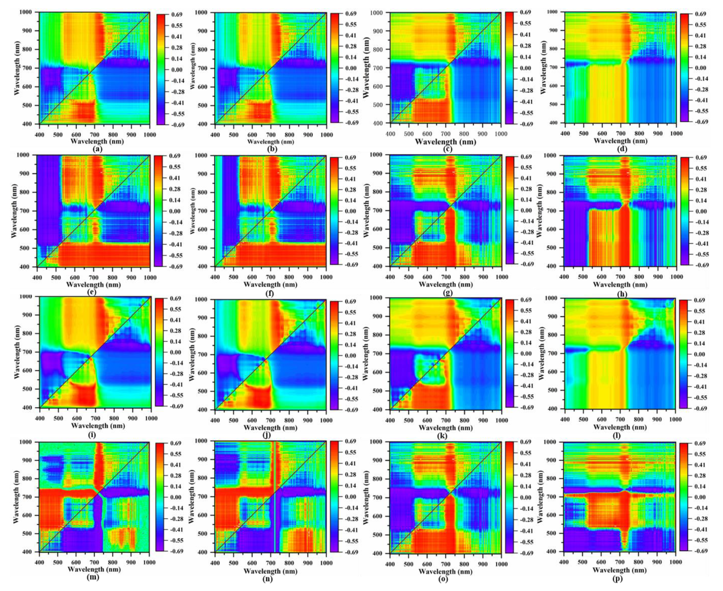
In this study, different growth period LAI changes and spectral responses were analyzed, and the results showed that with the increase of the growth period, LAI increased, while LAI of early-maturing varieties decreased at the floc opening stage and LAI of late-maturing varieties tended to remain unchanged, which was caused by the gradual cessation of vegetative growth and the drop of aging leaves at the later stage of crop growth. In terms of spectral response, LAI in the visible region was negatively correlated with canopy spectral reflectance, while LAI in the near-infrared region was positively correlated with canopy spectral reflectance, which is consistent with previous studies on winter wheat [44], rice [45], and rape [32]. This is due to the spectral reflectance of vegetation. The difference in the 350–800 nm range is mainly due to the influence of chlorophyll and other pigments in plants, and the difference in the 800–1000 nm range is due to the scattering of plant cells and tissues. Cotton growing luxuriantly and multi-leaf superimposed radiation will produce high reflectance in the near-infrared band. Therefore, canopy spectra of different LAI values differ more significantly in the near-infrared region.
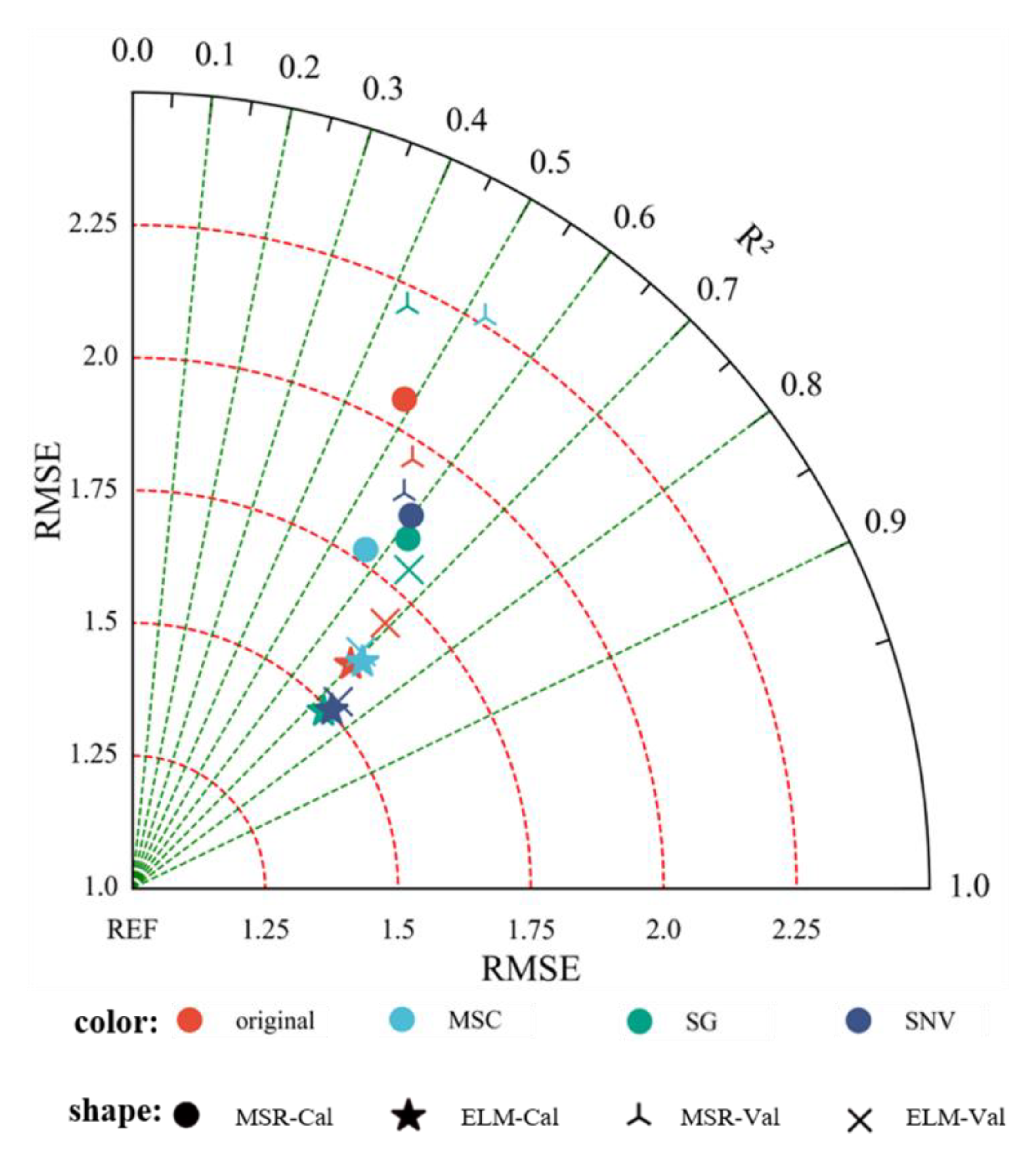
The original canopy spectrum is affected by the solar radiation flux, crop structure characteristics, and soil background conditions [46]. Spectral pretreatment can reduce background noise information and effectively improve the accuracy of spectral information [34]. Previous studies have shown that SNV can be used to eliminate the interference caused by light scattering and path length changes, and it can better predict the monitoring of the P and K content in tea [47]. Rei et al. [48] estimated the chlorophyll content after treating the original canopy spectrum with different methods, and the results showed that SNV and MSC did not show better performance. This is in contrast to this study’s results, which is potentially related to the spectral data in this study being obtained from UAV sensors, to atmospheric differences, to unmanned aerial vehicle (UAV) flight patterns and noise, or to the Rei blade clip being used to obtain spectral data, which did not require further correction.
The hyperspectral analysis includes two steps: characteristic band screening and regression modeling [49]. In this study, LAI-sensitive bands were screened out using SPA and SFLA, and the results showed that the model based on SFLA had better performance. Ren et al. [50] compared four band screening methods to grade black tea. Li et al. [51] estimated soil arsenic content on the basis of hyperspectral data, obtaining similar results in this study. This is because, compared with the SPA algorithm, SFLA is a novel method of forwarding variable cyclic selection. The maximum projection vector wavelength is taken as the combination of candidate wavelengths, and the correction is made on this basis. In combination with the modeling method, acceptable prediction results are obtained on the spectrum, and better generalization performance can be obtained by reducing the data dimension, which has broad application potential. In the existing research models, band screening effectively reduced the data dimensionality, but the traditional linear regression modeling still had collinearity problems.
Artificial intelligence (AI) coupled with promising machine learning (ML) techniques well known from computer science is broadly affecting many aspects of various fields, including science and technology, industry, and even our day-to-day life [52]. In recent years, in order to better realize the monitoring of cotton growth information, some scholars introduced machine vision, deep learning, and other technologies, which effectively improved the monitoring model accuracy [11,
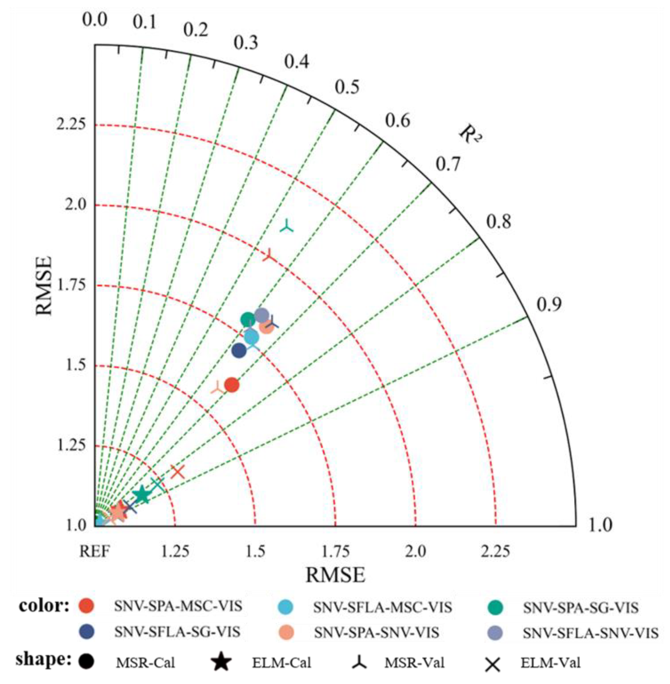
53]. In this study, the LAI monitoring model was established by comparing MSR and ELM algorithms, and the results showed that ELM was superior to MSR. The SNV-SFLA-ELM model has the best accuracy (R2 = 0.7340, RMSE = 1.4494, and rRMSE = 23.40%; verification set R2 = 0.7153, RMSE = 1.6796, and rRMSE = 26.32%), Yu et al. [54] compared PLSR and ELM to construct a hyperspectral inversion model of nitrogen content in rice leaves, and the results showed that ELM had better performance. Chen et al. [55] diagnosed the nitrogen content in the apple canopy on the basis of hyperspectral reflectance. Liu et al. [56] estimated rice chlorophyll content on the basis of hyperspectral reflectance, and the ELM model had the best effect. Meanwhile, the above study results show that ELM has a small computation scale and good generalization, but its practical application is slow. In this study, the ELM model also showed good prediction ability, but it needs to be improved for future research and application.
The model established in this study can be used for monitoring LAI throughout the growth period of cotton, including different cotton varieties. Chen et al. [57] established LAI monitoring models for cotton at different growth stages using multispectral data obtained by UAV, with R2 = 0.65 and RMSE = 0.62, similar to the performance of the monitoring model established on the basis of vegetation indices in this study. Hyperspectral reflectance can directly reflect the geometric and physiological characteristics of vegetation, and vegetation indices can quantitatively describe plant growth through the difference of vegetation and soil background in different band ranges. They are homologous but have different characteristic emphases. Therefore, in order to improve the accuracy of the model, canopy spectral reflectance and vegetation indices were combined to construct the model in this study, and more sensors and modeling methods could be introduced to monitor the model construction in the future.
In summary, SNV pretreatment was used for spectral data and SFLA was used to screen sensitive bands, which could optimize model variables. However, the correlation between vegetation indices established by spectral reflectance after SNV pretreatment and LAI was higher, which could improve model accuracy. ELM can effectively resist noise and is more suitable for modeling remote sensing data. The SNV-SFLA-SNV-VIs model was the optimal model established in this study, with training set R2 = 0.9208, RMSE = 0.8216, and rRMSE = 12.89%, and validation set R2 = 0.9066, RMSE = 0.9590, and rRMSE = 15.72%. In order to determine the predictive ability of the model in different periods, the model was verified in different periods in this study. The results showed that the accuracy of the validation model based on a single period decreased, but the overall accuracy was high, while LAI that was too large or too small had a greater error in estimation. Thus, although this model has a broad application prospect in monitoring LAI during the whole growth period of cotton, future studies still need to add data sets on this basis to ensure the universality of the model. In addition, this study based on the optimal model of different N application levels of LAI estimation ability test, the results show that the model under different nitrogen levels estimate ability has significant differences. Under different nitrogen levels, the N4 interchange and N2 precision is relatively low and, combined with the model, may be related to the LAI distribution under different nitrogen treatment. The model for larger LAI will be underestimated, while for smaller LAI, overestimation will occur. The research on this part is relatively weak, which is an important issue to be paid attention to in the future model construction and optimization process.
In this study, different nitrogen treatments and different cotton varieties were established, but the method in this study was based on the spectral data of a cotton canopy in the same year at a specific site, which limits its prediction ability for other datasets or regions. Therefore, in order to optimize the SNV-SFLA-SNV-VIs model in terms of stability and accuracy, further datasets involving additional years, planting patterns, and regions need to be collected for model correction, in order to realize LAI estimation of cotton in Xinjiang by using a machine learning method in the future.

5. Conclusions

In this study, using the spectral data of cotton canopy height obtained by UAV, band combinations were screened using different pretreatment and band screening methods, and vegetation indices were constructed using hyperspectral data after different pretreatment methods were used to estimate the LAI of cotton throughout the growth period using MSR and ELM. The results showed that the canopy spectra of different LAI were significantly different in the 760–1000 nm range, and there was an obvious correlation between the canopy spectrum and LAI. By comparing methods under different pretreatments, it can be seen that the band screening based on SPA was too concentrated, resulting in information redundancy and incomplete information extraction. The sensitive bands screened by SFLA were evenly distributed. The vegetation index established based on the hyperspectral data pretreated by SNV had a higher correlation with LAI, and the DVI had the highest correlation. In comparing the results of the cotton LAI estimation model established using two modeling methods based on different modeling objects, ELM was superior to MSR. SNV-SFLA was the best monitoring model based on pretreated hyperspectral reflectance, and SNV was the best monitoring model based on vegetation indices. However, when combining hyperspectral reflectance with vegetation indices, the ELM model based on SNV-SFLA-SNV-VIs had the best effect among all models, with training set R2 = 0.9208, RMSE = 0.8216, and rRMSE = 12.89%, and validation set R2 = 0.9066, RMSE = 0.9590, and rRMSE = 15.72%. Therefore, the combination of both modeling objects could effectively improve the model’s accuracy.

Author Contributions

Conceptualization, Y.M., Z.Z. and L.Z.; methodology, Y.M.; validation, Y.M., X.Y. and C.H.; formal analysis, Q.Z. and Y.M.; investigation, L.M. and X.Y.; resources, C.H., L.Z., Z.Z. and X.L.; data curation, Q.Z. and X.Y.; writing—original draft preparation, Y.M.; writing—review and editing, Y.M., Q.Z., Z.Z. and C.H.; funding acquisition, Z.Z., X.L. and C.H. All authors have read and agreed to the published version of the manuscript.

Funding

This study was supported by the National Natural Science Foundation of China (No. 42061658; 41971321), Key Research Program of Frontier Sciences, CAS (No. ZDBS-LY-DQC012), Key Scientific and Technological Research Program of XPCC(No. 2020AB005); Major Science and Technology Project of the Corps(No. 2018AA004).

Institutional Review Board Statement

Not applicable.

Informed Consent Statement

Not applicable.

Data Availability Statement

Not report any data.

Acknowledgments

The authors thank co-first author Qiang Zhang for his contributions to article writing and data curation. In addition, I would like to thank Bing Chen for their assistance in testing data collection and farmland management.

Conflicts of Interest

The authors declare that the research was conducted in the absence of any commercial or financial relationships that could be construed as a potential conflict of interest.

References

  1. Khan, M.A.; Wahid, A.; Ahmad, M.; Tahir, M.T.; Ahmed, M.; Ahmad, S.; Hasanuzzaman, M. World Cotton Production and Consumption: An Overview. In Cotton Production and Uses: Agronomy, Crop Protection, and Postharvest Technologies; Ahmad, S., Hasanuzzaman, M., Eds.; Springer: Singapore, 2020; pp. 1–7. ISBN 9789811514722. [Google Scholar]
  2. Muharam, F.M.; Delahunty, T.; Maas, S.J. Evaluation of Nitrogen Treatment Effects on the Reflectance of Cotton at Different Spatial Scales. Int. J. Remote Sens. 2018, 39, 8482–8504. [Google Scholar] [CrossRef]
  3. Rochester, I.J.; Constable, G.A.; Rochester, I.J.; Constable, G.A. Nitrogen-Fertiliser Application Effects on Cotton Lint Percentage, Seed Size, and Seed Oil and Protein Concentrations. Crop Pasture Sci. 2020, 71, 831–836. [Google Scholar] [CrossRef]
  4. Snider, J.; Harris, G.; Roberts, P.; Meeks, C.; Chastain, D.; Bange, M.; Virk, G. Cotton Physiological and Agronomic Response to Nitrogen Application Rate. Field Crops Res. 2021, 270, 108194. [Google Scholar] [CrossRef]
  5. Tao, H.; Feng, H.; Xu, L.; Miao, M.; Long, H.; Yue, J.; Li, Z.; Yang, G.; Yang, X.; Fan, L. Estimation of Crop Growth Parameters Using UAV-Based Hyperspectral Remote Sensing Data. Sensors 2020, 20, 1296. [Google Scholar] [CrossRef] [Green Version]
  6. An, M.; Xing, W.; Han, Y.; Bai, Q.; Peng, Z.; Zhang, B.; Wei, Z.; Wu, W. The Optimal Soil Water Content Models Based on Crop-LAI and Hyperspectral Data of Winter Wheat. Irrig. Sci. 2021, 39, 687–701. [Google Scholar] [CrossRef]
  7. Revill, A.; Myrgiotis, V.; Florence, A.; Hoad, S.; Rees, R.; MacArthur, A.; Williams, M. Combining Process Modelling and LAI Observations to Diagnose Winter Wheat Nitrogen Status and Forecast Yield. Agronomy 2021, 11, 314. [Google Scholar] [CrossRef]
  8. Shi, P.; Wang, Y.; Xu, J.; Zhao, Y.; Yang, B.; Yuan, Z.; Sun, Q. Rice Nitrogen Nutrition Estimation with RGB Images and Machine Learning Methods. Comput. Electron. Agric. 2021, 180, 105860. [Google Scholar] [CrossRef]
  9. Zhu, Y.; Zhao, C.; Yang, H.; Yang, G.; Han, L.; Li, Z.; Feng, H.; Xu, B.; Wu, J.; Lei, L. Estimation of Maize Above-Ground Biomass Based on Stem-Leaf Separation Strategy Integrated with LiDAR and Optical Remote Sensing Data. PeerJ 2019, 7, e7593. [Google Scholar] [CrossRef] [PubMed] [Green Version]
  10. Haldar, D.; Dave, V.; Misra, A.; Bhattacharya, B. Radar Vegetation Index for Assessing Cotton Crop Condition Using RISAT-1 Data. Geocarto Int. 2020, 35, 364–375. [Google Scholar] [CrossRef]
  11. Zhang, Y.; Xia, C.; Zhang, X.; Cheng, X.; Feng, G.; Wang, Y.; Gao, Q. Estimating the Maize Biomass by Crop Height and Narrowband Vegetation Indices Derived from UAV-Based Hyperspectral Images. Ecol. Indic. 2021, 129, 107985. [Google Scholar] [CrossRef]
  12. Xie, Q.; Dash, J.; Huete, A.; Jiang, A.; Yin, G.; Ding, Y.; Peng, D.; Hall, C.C.; Brown, L.; Shi, Y.; et al. Retrieval of Crop Biophysical Parameters from Sentinel-2 Remote Sensing Imagery. Int. J. Appl. Earth Obs. Geoinf. 2019, 80, 187–195. [Google Scholar] [CrossRef]
  13. Qiao, L.; Gao, D.; Zhang, J.; Li, M.; Sun, H.; Ma, J. Dynamic Influence Elimination and Chlorophyll Content Diagnosis of Maize Using UAV Spectral Imagery. Remote Sens. 2020, 12, 2650. [Google Scholar] [CrossRef]
  14. Zhang, L.; Han, W.; Niu, Y.; Chávez, J.L.; Shao, G.; Zhang, H. Evaluating the Sensitivity of Water Stressed Maize Chlorophyll and Structure Based on UAV Derived Vegetation Indices. Comput. Electron. Agric. 2021, 185, 106174. [Google Scholar] [CrossRef]
  15. Thorp, K.; Thompson, A.; Harders, S.; French, A.; Ward, R. High-Throughput Phenotyping of Crop Water Use Efficiency via Multispectral Drone Imagery and a Daily Soil Water Balance Model. Remote Sens. 2018, 10, 1682. [Google Scholar] [CrossRef] [Green Version]
  16. Tavakoli, H.; Gebbers, R. Assessing Nitrogen and Water Status of Winter Wheat Using a Digital Camera. Comput. Electron. Agric. 2019, 157, 558–567. [Google Scholar] [CrossRef]
  17. Yang, M.; Hassan, M.A.; Xu, K.; Zheng, C.; Rasheed, A.; Zhang, Y.; Jin, X.; Xia, X.; Xiao, Y.; He, Z. Assessment of Water and Nitrogen Use Efficiencies Through UAV-Based Multispectral Phenotyping in Winter Wheat. Front. Plant Sci. 2020, 11, 927. [Google Scholar] [CrossRef]
  18. Marang, I.J.; Filippi, P.; Weaver, T.B.; Evans, B.J.; Whelan, B.M.; Bishop, T.F.A.; Murad, M.O.F.; Al-Shammari, D.; Roth, G. Machine Learning Optimised Hyperspectral Remote Sensing Retrieves Cotton Nitrogen Status. Remote Sens. 2021, 13, 1428. [Google Scholar] [CrossRef]
  19. Dong, T.; Liu, J.; Shang, J.; Qian, B.; Ma, B.; Kovacs, J.M.; Walters, D.; Jiao, X.; Geng, X.; Shi, Y. Assessment of Red-Edge Vegetation Indices for Crop Leaf Area Index Estimation. Remote Sens. Environ. 2019, 222, 133–143. [Google Scholar] [CrossRef]
  20. Cheng, Z.; Meng, J.; Shang, J.; Liu, J.; Huang, J.; Qiao, Y.; Qian, B.; Jing, Q.; Dong, T.; Yu, L. Generating Time-Series LAI Estimates of Maize Using Combined Methods Based on Multispectral UAV Observations and WOFOST Model. Sensors 2020, 20, 6006. [Google Scholar] [CrossRef] [PubMed]
  21. Fang, H.; Baret, F.; Plummer, S.; Schaepman-Strub, G. An Overview of Global Leaf Area Index (LAI): Methods, Products, Validation, and Applications. Rev. Geophys. 2019, 57, 739–799. [Google Scholar] [CrossRef]
  22. Yu, L.; Shang, J.; Cheng, Z.; Gao, Z.; Wang, Z.; Tian, L.; Wang, D.; Che, T.; Jin, R.; Liu, J.; et al. Assessment of Cornfield LAI Retrieved from Multi-Source Satellite Data Using Continuous Field LAI Measurements Based on a Wireless Sensor Network. Remote Sens. 2020, 12, 3304. [Google Scholar] [CrossRef]
  23. Dong, T.; Liu, J.; Qian, B.; He, L.; Liu, J.; Wang, R.; Jing, Q.; Champagne, C.; McNairn, H.; Powers, J.; et al. Estimating Crop Biomass Using Leaf Area Index Derived from Landsat 8 and Sentinel-2 Data. ISPRS J. Photogramm. Remote Sens. 2020, 168, 236–250. [Google Scholar] [CrossRef]
  24. Caballero, D.; Calvini, R.; Amigo, J.M. Chapter 3.3—Hyperspectral Imaging in Crop Fields: Precision Agriculture. In Data Handling in Science and Technology; Amigo, J.M., Ed.; Hyperspectral Imaging; Elsevier: Amsterdam, The Netherlands, 2020; Volume 32, pp. 453–473. [Google Scholar]
  25. Gaso, D.V.; de Wit, A.; Berger, A.G.; Kooistra, L. Predicting Within-Field Soybean Yield Variability by Coupling Sentinel-2 Leaf Area Index with a Crop Growth Model. Agric. For. Meteorol. 2021, 308–309, 108553. [Google Scholar] [CrossRef]
  26. Li, S.; Yuan, F.; Ata-UI-Karim, S.T.; Zheng, H.; Cheng, T.; Liu, X.; Tian, Y.; Zhu, Y.; Cao, W.; Cao, Q. Combining Color Indices and Textures of UAV-Based Digital Imagery for Rice LAI Estimation. Remote Sens. 2019, 11, 1763. [Google Scholar] [CrossRef] [Green Version]
  27. Pasqualotto, N.; Delegido, J.; Van Wittenberghe, S.; Rinaldi, M.; Moreno, J. Multi-Crop Green LAI Estimation with a New Simple Sentinel-2 LAI Index (SeLI). Sensors 2019, 19, 904. [Google Scholar] [CrossRef] [PubMed] [Green Version]
  28. Wang, J.; Xiao, X.; Bajgain, R.; Starks, P.; Steiner, J.; Doughty, R.B.; Chang, Q. Estimating Leaf Area Index and Aboveground Biomass of Grazing Pastures Using Sentinel-1, Sentinel-2 and Landsat Images. ISPRS J. Photogramm. Remote Sens. 2019, 154, 189–201. [Google Scholar] [CrossRef] [Green Version]
  29. Zhang, J.; Cheng, T.; Guo, W.; Xu, X.; Qiao, H.; Xie, Y.; Ma, X. Leaf Area Index Estimation Model for UAV Image Hyperspectral Data Based on Wavelength Variable Selection and Machine Learning Methods. Plant Methods 2021, 17, 49. [Google Scholar] [CrossRef]
  30. Duan, B.; Liu, Y.; Gong, Y.; Peng, Y.; Wu, X.; Zhu, R.; Fang, S. Remote Estimation of Rice LAI Based on Fourier Spectrum Texture from UAV Image. Plant. Methods 2019, 15, 1–12. [Google Scholar] [CrossRef] [Green Version]
  31. Qiao, L.; Gao, D.; Zhao, R.; Tang, W.; An, L.; Li, M.; Sun, H. Improving Estimation of LAI Dynamic by Fusion of Morphological and Vegetation Indices Based on UAV Imagery. Comput. Electron. Agric. 2022, 192, 106603. [Google Scholar] [CrossRef]
  32. Peng, Y.; Zhu, T.; Li, Y.; Dai, C.; Fang, S.; Gong, Y.; Wu, X.; Zhu, R.; Liu, K. Remote Prediction of Yield Based on LAI Estimation in Oilseed Rape under Different Planting Methods and Nitrogen Fertilizer Applications. Agric. For. Meteorol. 2019, 271, 116–125. [Google Scholar] [CrossRef]
  33. Yuan, H.; Yang, G.; Li, C.; Wang, Y.; Liu, J.; Yu, H.; Feng, H.; Xu, B.; Zhao, X.; Yang, X. Retrieving Soybean Leaf Area Index from Unmanned Aerial Vehicle Hyperspectral Remote Sensing: Analysis of RF, ANN, and SVM Regression Models. Remote Sens. 2017, 9, 309. [Google Scholar] [CrossRef] [Green Version]
  34. Li, L.; Lin, D.; Wang, J.; Yang, L.; Wang, Y. Multivariate Analysis Models Based on Full Spectra Range and Effective Wavelengths Using Different Transformation Techniques for Rapid Estimation of Leaf Nitrogen Concentration in Winter Wheat. Front. Plant Sci. 2020, 11, 755. [Google Scholar] [CrossRef] [PubMed]
  35. Yang, X.; Bao, N.; Li, W.; Liu, S.; Fu, Y.; Mao, Y. Soil Nutrient Estimation and Mapping in Farmland Based on UAV Imaging Spectrometry. Sensors 2021, 21, 3919. [Google Scholar] [CrossRef] [PubMed]
  36. Han, X.; Wei, Z.; Chen, H.; Zhang, B.; Li, Y.; Du, T. Inversion of Winter Wheat Growth Parameters and Yield Under Different Water Treatments Based on UAV Multispectral Remote Sensing. Front. Plant. Sci. 2021, 12, 639. [Google Scholar] [CrossRef] [PubMed]
  37. Yao, X.; Wang, N.; Liu, Y.; Cheng, T.; Tian, Y.; Chen, Q.; Zhu, Y. Estimation of Wheat LAI at Middle to High Levels Using Unmanned Aerial Vehicle Narrowband Multispectral Imagery. Remote Sens. 2017, 9, 1304. [Google Scholar] [CrossRef] [Green Version]
  38. Rehman, T.U.; Mahmud, M.S.; Chang, Y.K.; Jin, J.; Shin, J. Current and Future Applications of Statistical Machine Learning Algorithms for Agricultural Machine Vision Systems. Comput. Electron. Agric. 2019, 156, 585–605. [Google Scholar] [CrossRef]
  39. Zha, H.; Miao, Y.; Wang, T.; Li, Y.; Zhang, J.; Sun, W.; Feng, Z.; Kusnierek, K. Improving Unmanned Aerial Vehicle Remote Sensing-Based Rice Nitrogen Nutrition Index Prediction with Machine Learning. Remote Sens. 2020, 12, 215. [Google Scholar] [CrossRef] [Green Version]
  40. Pettorelli, N. The Normalized Difference Vegetation Index; OUP: Oxford, UK, 2013; ISBN 978-0-19-969316-0. [Google Scholar]
  41. Richardson, A.J.; Weigand, C.L. Distinguishing Vegetation from Soil Background Information. Photogramm. Eng. Remote Sens. 1977, 43, 1541–1552. [Google Scholar]
  42. Geladi, P.; Kowalski, B.R. Partial Least-Squares Regression: A Tutorial. Anal. Chim. Acta 1986, 185, 1–17. [Google Scholar] [CrossRef]
  43. Jordan, M.I.; Mitchell, T.M. Machine Learning: Trends, Perspectives, and Prospects. Science 2015, 349, 255–260. [Google Scholar] [CrossRef]
  44. Li, X.; Zhang, Y.; Bao, Y.; Luo, J.; Jin, X.; Xu, X.; Song, X.; Yang, G. Exploring the Best Hyperspectral Features for LAI Estimation Using Partial Least Squares Regression. Remote Sens. 2014, 6, 6221–6241. [Google Scholar] [CrossRef] [Green Version]
  45. Din, M.; Zheng, W.; Rashid, M.; Wang, S.; Shi, Z. Evaluating Hyperspectral Vegetation Indices for Leaf Area Index Estimation of Oryza Sativa L. at Diverse Phenological Stages. Front. Plant Sci. 2017, 8, 820. [Google Scholar] [CrossRef] [Green Version]
  46. Baldocchi, D.D.; Ryu, Y.; Dechant, B.; Eichelmann, E.; Hemes, K.; Ma, S.; Sanchez, C.R.; Shortt, R.; Szutu, D.; Valach, A.; et al. Outgoing Near-Infrared Radiation From Vegetation Scales With Canopy Photosynthesis Across a Spectrum of Function, Structure, Physiological Capacity, and Weather. J. Geophys. Res. Biogeosci. 2020, 125, e2019JG005534. [Google Scholar] [CrossRef]
  47. Wang, Y.-J.; Jin, G.; Li, L.-Q.; Liu, Y.; Kianpoor Kalkhajeh, Y.; Ning, J.-M.; Zhang, Z.-Z. NIR Hyperspectral Imaging Coupled with Chemometrics for Nondestructive Assessment of Phosphorus and Potassium Contents in Tea Leaves. Infrared Phys. Technol. 2020, 108, 103365. [Google Scholar] [CrossRef]
  48. Sonobe, R.; Yamashita, H.; Mihara, H.; Morita, A.; Ikka, T. Estimation of Leaf Chlorophyll a, b and Carotenoid Contents and Their Ratios Using Hyperspectral Reflectance. Remote Sens. 2020, 12, 3265. [Google Scholar] [CrossRef]
  49. Rasti, B.; Hong, D.; Hang, R.; Ghamisi, P.; Kang, X.; Chanussot, J.; Benediktsson, J.A. Feature Extraction for Hyperspectral Imagery: The Evolution From Shallow to Deep: Overview and Toolbox. IEEE Geosci. Remote Sens. Mag. 2020, 8, 60–88. [Google Scholar] [CrossRef]
  50. Ren, G.; Wang, Y.; Ning, J.; Zhang, Z. Highly Identification of Keemun Black Tea Rank Based on Cognitive Spectroscopy: Near Infrared Spectroscopy Combined with Feature Variable Selection. Spectrochim. Acta Part A Mol. Biomol. Spectrosc. 2020, 230, 118079. [Google Scholar] [CrossRef]
  51. Han, L.; Chen, R.; Zhu, H.; Zhao, Y.; Liu, Z.; Huo, H. Estimating Soil Arsenic Content with Visible and Near-Infrared Hyperspectral Reflectance. Sustainability 2020, 12, 1476. [Google Scholar] [CrossRef] [Green Version]
  52. Xu, Y.; Liu, X.; Cao, X.; Huang, C.; Liu, E.; Qian, S.; Liu, X.; Wu, Y.; Dong, F.; Qiu, C.-W.; et al. Artificial Intelligence: A Powerful Paradigm for Scientific Research. Innovation 2021, 2, 100179. [Google Scholar] [CrossRef]
  53. Paul, A.; Ghosh, S.; Das, A.K.; Goswami, S.; Das Choudhury, S.; Sen, S. A Review on Agricultural Advancement Based on Computer Vision and Machine Learning. In Proceedings of the Emerging Technology in Modelling and Graphics; Mandal, J.K., Bhattacharya, D., Eds.; Springer: Singapore, 2020; pp. 567–581. [Google Scholar]
  54. Yu, F.; Feng, S.; Du, W.; Wang, D.; Guo, Z.; Xing, S.; Jin, Z.; Cao, Y.; Xu, T. A Study of Nitrogen Deficiency Inversion in Rice Leaves Based on the Hyperspectral Reflectance Differential. Front. Plant Sci. 2020, 11, 1758. [Google Scholar] [CrossRef]
  55. Chen, S.; Hu, T.; Luo, L.; He, Q.; Zhang, S.; Li, M.; Cui, X.; Li, H. Rapid Estimation of Leaf Nitrogen Content in Apple-Trees Based on Canopy Hyperspectral Reflectance Using Multivariate Methods. Infrared Phys. Technol. 2020, 111, 103542. [Google Scholar] [CrossRef]
  56. Wang, X.; Miao, Y.; Dong, R.; Zha, H.; Xia, T.; Chen, Z.; Kusnierek, K.; Mi, G.; Sun, H.; Li, M. Machine Learning-Based in-Season Nitrogen Status Diagnosis and Side-Dress Nitrogen Recommendation for Corn. Eur. J. Agron. 2021, 123, 126193. [Google Scholar] [CrossRef]
  57. Chen, P. Cotton Leaf Area Index Estimation Using Unmanned Aerial Vehicle Multi-Spectral Images. In Proceedings of the IGARSS 2019—2019 IEEE International Geoscience and Remote Sensing Symposium, Yokohama, Japan, 28 July–2 August 2019; pp. 6251–6254. [Google Scholar]
Figure 1. Study area survey: (a) location of study site; (b) study area1 plant Xinluzao 53 and Xinluzao 43, study area2 plant Luyanmian 24; (c) the level of nitrogen fertilizer in each area. Note: N0 represents nitrogen application of 0 kg/hm2, N1 represents nitrogen application of 120 kg/hm2, N2 represents nitrogen application of 240 kg/hm2, NC represents nitrogen application of 360 kg/hm2, N3 represents nitrogen application of 480 kg/hm2, and N4 represents nitrogen application of 600 kg/hm2.
Remotesensing 14 00136 g001
Figure 2. (a) Xinluzao 53 leaf area index and spectral difference of cultivars at different growth stages, (b) Xinluzao 45 leaf area index and spectral difference of cultivars at different growth stages, (c) Luyanmian 24 leaf area index and spectral difference of cultivars at different growth stages, (d) cotton canopy reflectance and (e) correlation analysis of cotton LAI index.
Remotesensing 14 00136 g002
Figure 3. SPA screening results: (a) OR-SPA, (b) SG-FDR-SPA, (c) SG-SDR-SPA, and (d) SNV-SPA.
Remotesensing 14 00136 g003
Figure 4. SFLA screening results: (a) OR-SPA, (b) SG-FDR-SPA, (c) SG-SDR-SPA, and (d) SNV-SPA.
Remotesensing 14 00136 g004
Figure 5. Screening results: (a) SPA and (b) SFLA.
Remotesensing 14 00136 g005
Figure 6. Vegetation index construction based on correlation matrix; different preprocessing spectral reflectance construction vegetation indices: (a) OR-NDVI, (b) OR-RVI, (c) OR-DVI, (d) OR-NIL, (e) MSC-NDVI, (f)MSC-RVI, (g) MSC-DVI, (h) MSC-NIL, (i) SG-NDVI, (j) SG-RVI, (k) SG-DVI, (l) SG-NIL, (m) SNV-NDVI, (n) SNV-RVI, (o) SNV-DVI, and (p) SNV-NIL.
Remotesensing 14 00136 g006
Figure 7. Cotton LAI monitoring model training sets (Cal) and validation sets (Val) result based on spectral reflectance: resultant Taylor diagram.
Remotesensing 14 00136 g007
Figure 8. Linear results of measured and predicted values based on spectral reflectance model training sets (Cal) and validation sets (Val): (a) MSR-SNV-SPA, (b) MSR-SNV-SFLA, (c) ELM-SNV-SPA, and (d) ELM-SNV-SFLA.
Remotesensing 14 00136 g008
Figure 9. Cotton LAI monitoring model training sets (Cal) and validation sets (Val) result based on vegetation indices: resultant Taylor diagram.
Remotesensing 14 00136 g009
Figure 10. Linear results of training sets (Cal) and validation sets (Val) measured and predicted values based on vegetation indices model: (a) MSR-SNV and (b) ELM-SNV.
Remotesensing 14 00136 g010
Figure 11. Cotton LAI monitoring model training sets (Cal) and validation sets (Val) result based on combination of spectral reflectance and vegetation indices: resultant Taylor diagram.
Remotesensing 14 00136 g011
Figure 12. Linear results of training sets (Cal) and validation sets (Val) measured and predicted values based on spectral reflectance and vegetation indices: (a) MSR-SNV-SPA-MSC-VIs, (b) MSR-SNV-SPA-SG-VIs, (c) MSR-SNV-SPA-SNV-VIs, (d) MSR-SNV-SFLA-MSC-VIs, (e) MSR-SNV-SFLA-SG-VIs, (f) MSR-SNV-SFLA-SNV-VIs, (g) ELM-SNV-SPA-MSC-VIs, (h) ELM-SNV-SPA-SG-VIs, (i) ELM-SNV-SPA-SNV-VIs, (j) ELM-SNV-SFLA-MSC-VIs, (k) ELM-SNV-SFLA-SG-VIs, and (l) ELM-SNV-SFLA-SNV-VIs.
Remotesensing 14 00136 g012
Figure 13. Model testing result. (a) Test accuracy of ELM-SNV-SFLA-SNV-VIs model under different sample times. (b) Test accuracy of ELM-SNV-SFLA-SNV-VIs model under different nitrogen application levels. (c) Optimal model external test results.
Remotesensing 14 00136 g013
Table 1. Crop management 2019.
ItemCotton
Sowing date24 April 2019
VarietyXinluzao 53, Xinluzao 45, Luyanmian 24
Harvest date15 October 2019
Soil typeHeavy loam
FertilizationWhole growing season: NH4PO3 390 kg/hm2, K2SO4 180 kg/hm2
IrrigationWhole growing season: total irrigation water 3525 m3
Table 2. Main parameters of Nano-Hyperspec sensor.
ParametersValues
Weight (kg)0.6
Spectral range (nm)400–1000
Number of channels270
Spectral sampling interval (nm)2.2
Table 3. Vegetation indices tested in this study.
Vegetation IndexesFormulaReference
Normalized difference vegetation index (NDVI) NDVI = R λ 1 R λ 2 R λ 1 + R λ 2 [40]
Ration vegetation index (RVI) RVI = R λ 1 R λ 2 [40]
Difference vegetation index (DVI) DVI = R λ 1 R λ 2 [41]
Nonlinear vegetation index (NLI) NLI = R λ 1 2 R λ 2 R λ 1 2 + R λ 2
Table 4. Descriptive statistics of cotton LAI from the study area.
TreatmentSamplesMeanMaxMinSDCV (%)
N0595.718411.11601.55792.375941.55%
N1596.261514.17881.80393.075549.12%
N2596.524816.73272.12763.176048.68%
NC566.519413.33531.99232.946445.19%
N3566.368812.51382.28982.829044.42%
N4566.230813.58701.90653.077449.39%
Table 5. Correlation and selected bands of optimal vegetation indices after spectral transformation.
PretreatmentVegetation Indices
NDVIRVIDVINIL
OR0.6885 (907,745)0.6558 (443,631)−0.5551 (538,531)0.4969 (893,747)
MSC0.7013 (907,745)−0.7009 (745,907)−0.7581 (540,525)0.7120 (907,745)
SG−0.6775 (640,436)0.6840 (436,640)−0.6868 (451,445)−0.3775 (989,996)
SNV−0.7176 (525,540)0.7186 (540,525)−0.7591 (540,525)0.7114 (907,745)
Table 6. Cotton LAI monitoring model training sets (Cal) and validation sets (Val) result based on spectral reflectance.
Modeling ApproachPre-ProcessingFeature SelectionCalVal
R2RMSErRMSER2RMSErRMSE
MSRoriginalSPA0.55412.004031.81%0.48062.045932.90%
SFLA0.56871.944229.97%0.49752.053234.57%
SG-FDRSPA0.51632.064033.26%0.49122.085332.79%
SFLA0.57241.968930.95%0.54571.905931.10%
SG-SDRSPA0.59331.935331.40%0.50981.953930.41%
SFLA0.54941.912630.22%0.59211.880930.83%
SNVSPA0.59621.933630.78%0.58501.798328.79%
SFLA0.60741.906630.35%0.59411.787328.61%
ELMoriginalSPA0.67551.582324.94%0.62701.939831.54%
SFLA0.70301.556924.32%0.64241.862030.72%
SG-FDRSPA0.69621.628326.09%0.65691.717227.21%
SFLA0.73771.562323.83%0.68071.600927.41%
SG-SDRSPA0.62801.785128.42%0.61051.854629.68%
SFLA0.71831.631625.90%0.68461.545924.88%
SNVSPA0.70591.496124.25%0.69911.755327.34%
SFLA0.73401.449423.40%0.71531.679626.32%
Table 7. Cotton LAI monitoring model result based on vegetation indices.
Modeling ApproachPre-ProcessingCalVal
R2RMSErRMSER2RMSErRMSE
MSRoriginal0.48532.054532.27%0.54641.965132.51%
MSC0.56591.775129.30%0.52552.263834.39%
SG0.61821.838528.94%0.42682.213336.05%
SNV0.59831.877128.93%0.56661.903732.06%
ELMoriginal0.69771.589425.22%0.68971.690227.19%
MSC0.71241.608025.39%0.69461.619926.27%
SG0.73381.490723.31%0.65551.794729.55%
SNV0.74571.503224.05%0.74081.523124.33%
Table 8. Cotton LAI monitoring model training sets (Cal) and validation sets (Val) result based on spectral reflectance and vegetation indices.
Modeling ApproachPre-ProcessingCalVal
R2RMSErRMSER2RMSErRMSE
MSRSNV-SPA-MSC-VIS0.69571.613226.23%0.54382.000931.05%
SNV-SFLA-MSC-VIS0.63801.765427.73%0.65871.748528.57%
SNV-SPA-SG-VIS0.59571.801429.10%0.54012.106933.00%
SNV-SFLA-SG-VIS0.63441.708227.46%0.65771.839929.02%
SNV-SPA-SNV-VIS0.65151.821229.15%0.66691.574024.99%
SNV-SFLA-SNV-VIS0.61981.838029.22%0.61801.785328.64%
ELMSNV-SPA-MSC-VIS0.84631.095017.22%0.83591.308621.34%
SNV-SFLA-MSC-VIS0.88181.018116.00%0.88880.981716.03%
SNV-SPA-SG-VIS0.83461.176319.07%0.83271.234819.23%
SNV-SFLA-SG-VIS0.87281.082416.92%0.87231.125818.48%
SNV-SPA-SNV-VIS0.87121.083817.45%0.86961.051016.54%
SNV-SFLA-SNV-VIS0.92080.821612.89%0.90660.959015.72%
Table 9. Cotton LAI monitoring verification results of different sample times in the optimal model.
ModelingSample TimesR2RMSErRMSE
ELM-SNV-SFLA-SNV-VIs57 DAYS0.85220.489616.98%
66 DAYS0.86570.811315.61%
76 DAYS0.88680.37537.07%
88 DAYS0.89200.26553.61%
98 DAYS0.88480.780310.48%
112 DAYS0.79291.094015.17%
Table 10. Cotton LAI monitoring verification results of different N concentrations in the optimal model.
ModelN LevelR2RMSErRMSE
ELM-SNV-SFLA-SNV-VIsN00.94680.765411.09%
N10.93510.717412.26%
N20.87060.919115.26%
N30.93301.017615.17%
N40.79901.006318.04%
NC0.95310.711110.41%
Publisher’s Note: MDPI stays neutral with regard to jurisdictional claims in published maps and institutional affiliations.

