Ionospheric Disturbances Observed Following the Ridgecrest Earthquake of 4 July 2019 in California, USA

Abstract

Earthquakes are known to generate disturbances in the ionosphere. Such disturbances, referred to as co-seismic ionospheric disturbances, or ionoquakes, were previously reported for large earthquakes with magnitudes $\mathrm{Mw}\ge$ 6.6. This paper reports ionoquakes associated with the Ridgecrest earthquakes of magnitude $(\mathrm{Mw}=6.4)$, that occurred on 4 July 2019 in California, USA. The ionoquakes manifested in total electron content (TEC) in the form of traveling ionospheric disturbances (TIDs) within 1 h from the mainshock onset. These seismic-origin TIDs have unique wave characteristics that distinguish them from TIDs of non-seismic origin arising from a moderate geomagnetic activity on the same day. Moreover, in the space-time domain of the detection of seismic-origin TIDs, TIDs are absent on the day before and day after the earthquake day. Their spectral characteristics relate them to the Earth’s normal modes and atmospheric resonance modes. We found the ground velocity associated with the mainshock, rather than the ground displacement, satisfies the threshold criteria for detectable ionoquakes in TEC measurements. Numerical simulation suggested that the coupled seismo–atmosphere–ionosphere (SAI) dynamics energized by the atmospheric waves are responsible for the generation of ionoquakes. This study’s findings demonstrate the potential of using TEC measurement to detect the ionospheric counterparts of moderate earthquakes.

1. Introduction

During earthquakes (EQs), a significant part of the seismic energy and momentum of the ground displacement transfers to the overlying atmosphere and ionosphere [1,2,3,4,5,6,7,8,9,10,11,12,13]. This seismo–atmosphere–ionosphere (SAI) coupling involves neutral and plasma waves that eventually give rise to disturbances in the ionosphere [14]. The co-seismic ionospheric disturbances (or ionoquakes) can be detected in the form of disturbances in ionospheric motion deduced from Doppler sounders [2,15] and disturbances in ionospheric total electron content (TEC) data deduced from the Global Navigation Satellite Systems (GNSSs) networks [16,17,18,19,20,21,22,23,24]. Though less sensitive than Doppler measurements in detecting ionoquakes, GNSS-TEC measurements are widely used for the detection of co-seismic perturbations owing to their continuous operation and wider spatial coverage [12,16]. Moreover, high-rate GNSS-TEC measurements can be employed for determining the seismic source parameters [10,25,26,27].

However, that not all EQs can generate perturbations large enough to be detected in the ionosphere. Past studies reported that only EQs with a moment magnitude ($\mathrm{Mw}$) larger than 6.8 can generate detectable ionoquakes [28]. However, in some cases, even smaller events can be detected. The $\mathrm{Mw}$ 6.6 Chuetsu-Oki earthquake of 16 July 2007 is the smallest event ever recorded in the ionosphere Cahyadi and Heki (2015) [29]. In terms of the ground displacement required to produce a detectable ionoquake in GNSS-TEC measurements, the threshold of about 0.3 m was established [29]. This threshold is much higher than the threshold of ∼0.1 mm for Doppler measurements [16,30]. Therefore, ionoquake detection by GNSS-TEC measurements is limited to only strong EQs, and their detection for those $\mathrm{Mw}<$ 6.6 has not been reported to date. This task is crucial for future possible applications of ionosphere-based methods for the detection of natural hazards.

The detectability of ionoquakes, especially for smaller EQs, can be significantly challenging in the presence of non-seismic-origin disturbances. For instance, those produced from tropospheric convection and geomagnetic storm share common spectral and propagation characteristics with ionoquakes [9]. Therefore, it is difficult to separate the co-seismic from non-seismic ionospheric disturbances. This task is crucial for future possible applications of ionosphere-based methods for the detection of natural hazards. However, until now, no such methods have been suggested.

In the present study, we investigated the ionospheric response to a moderate EQ occurred in California, USA, on 4 July 2019. The magnitudes of the EQ was 6.4, i.e., below the previously reported threshold of 6.6–6.8 [28,29]. We note that the considered event occurred during moderate geomagnetic disturbances and before the strong EQ of $\mathrm{Mw}$ 7.1 on 6 July 2019. Therefore, this seismic event provided an ideal candidate for examining the potential of GNSS-TEC-based ionospheric seismology.

2. Materials and Methods

2.1. The 4 July 2019 Ridgecrest Earthquakes

On 4 July 2019 (referred as the event day), a moderate EQ with magnitude $\mathrm{Mw}$ 6.4 (the mainshock) occurred in eastern California (USA), north and northeast of the town of Ridgecrest. The mainshock struck at 17:33 UT, and a series of aftershocks followed during the next two hours (

Table 1. Selected earthquakes of the Ridgecrest sequence, USGS database, magnitude ≥ 3.55, 4 July 2019, California, USA.

No.	Time (UT)	Lat, Lon (Degrees)	Depth (km)	Magnitude	Location
1	17:33:49	35.71, −117.50	10.50	6.40	Ridgecrest Earthquake Sequence
2	18:08:45	35.71, 35.71	117.47	3.55	9 km SW of Searles Vallay
3	18:27:59	35.75, −117.55	6.64	4.23	14 km W of Searles Valley
4	18:39:44	35.60, −117.60	2.81	4.59	7 km ESE of Ridgecrest
5	18:47:06	35.67, −117.49	8.53	4.34	13 km SW of Searles Valley
6	18:54:13	35.60, −117.60	5.33	4.07	7 km ESE of Ridgecrest
7	18:56:06	35.72, −117.56	1.92	4.58	15 km NE of Ridgecrest
8	18:56:22	35.71, −117.55	1.16	4.21	15 km NE of Ridgecrest
9	19:21:32	35.67, −117.49	5.16	4.50	13 km SSW of Searles Valley

). The mainshock was the consequence of three separate EQs ($\mathrm{Mw}$ = 6.1, 6.2, and 6.2) in a trio of failures, lasting 12 s. Together, these produced enough energy to create a $\mathrm{Mw}$ 6.4 earthquake [31]. According to the U.S. Geological Survey (USGS), the mainshock resulted from shallow strike slip faulting (https://earthquake.usgs.gov/earthquakes/eventpage/ci38443183/technical (accessed on 5 November 2021)), which means that the co-seismic crustal displacements were mostly horizontal. The shakemap of the mainshock in Figure A1 (Appendix A) reveals that the seismic activity wasconfined in region between 117°–118° W and 35°–36° N.

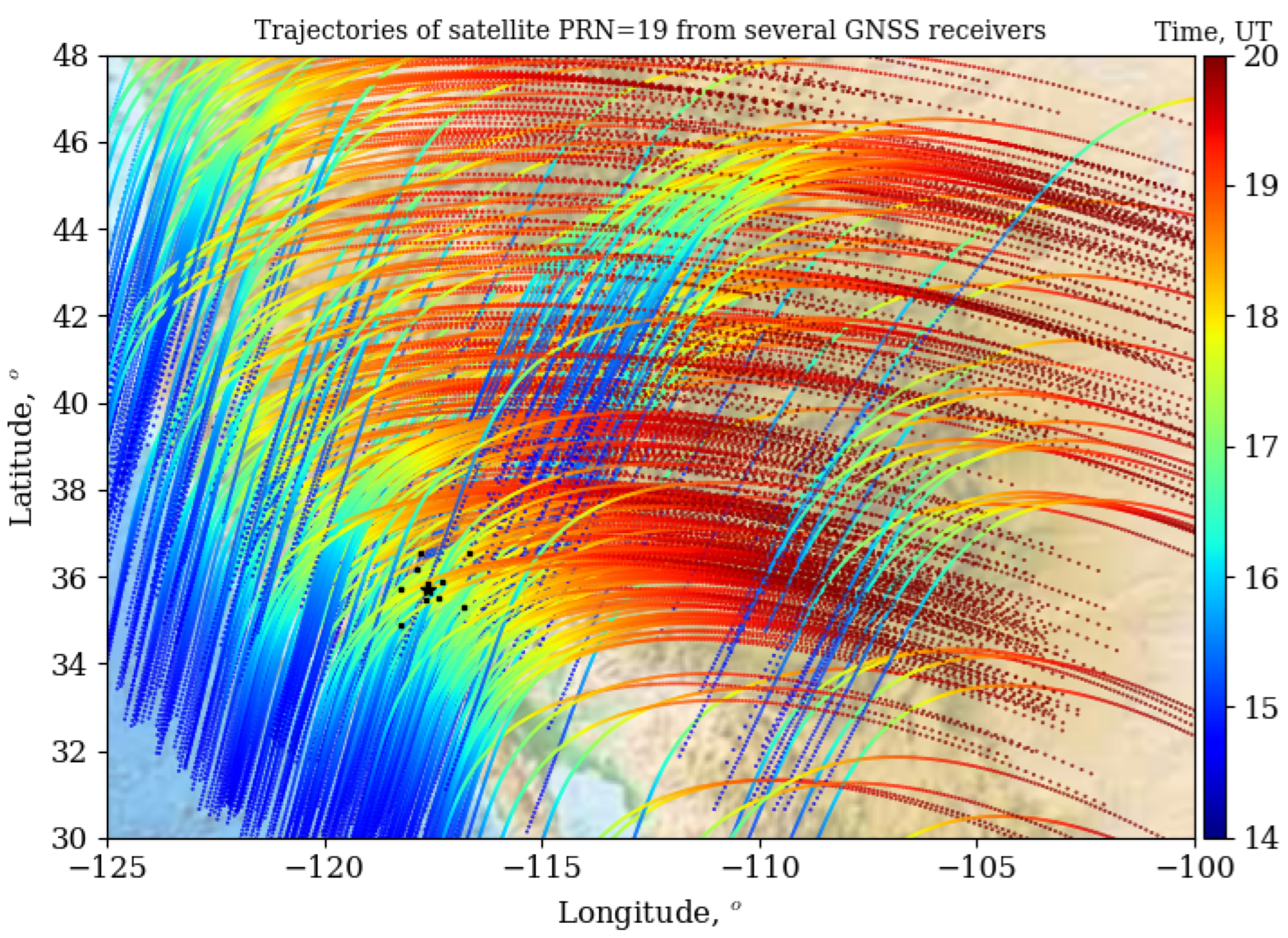
2.2. GNSS and Seismometer Data

In this study, we used 600 GNSS receivers near the epicenter of the earthquake of the permanent ground-based network UNAVCO (http://www.unavco.org (accessed on 5 November 2021)). The measurements provide phase and range characteristics of the radio signal transmitted from the GNSS satellites at two frequencies ($f_1$ = 1575.42 MHz and $f_2$ = 1227.60 MHz). These data are available in RINEX format with a sampling interval of 15 s. Satellite PRN19 was selected for the present analysis because the corresponding ionospheric piercing point (IPP) trajectories i.e., the trajectories of the satellite projected at the ionospheric height of 250 km, cover the earthquake shake zone around epicenter during the earthquakes (17:33:49 UT and 18:39:44 UT), as evident from Figure 1.

We also used data from the 10 ground seismometer stations with sampling of 0.025 s, located within 1° of the epicentral distance (IRIS network: http://ds.iris.edu/wilber3/find_event (accessed on 5 November 2021)).

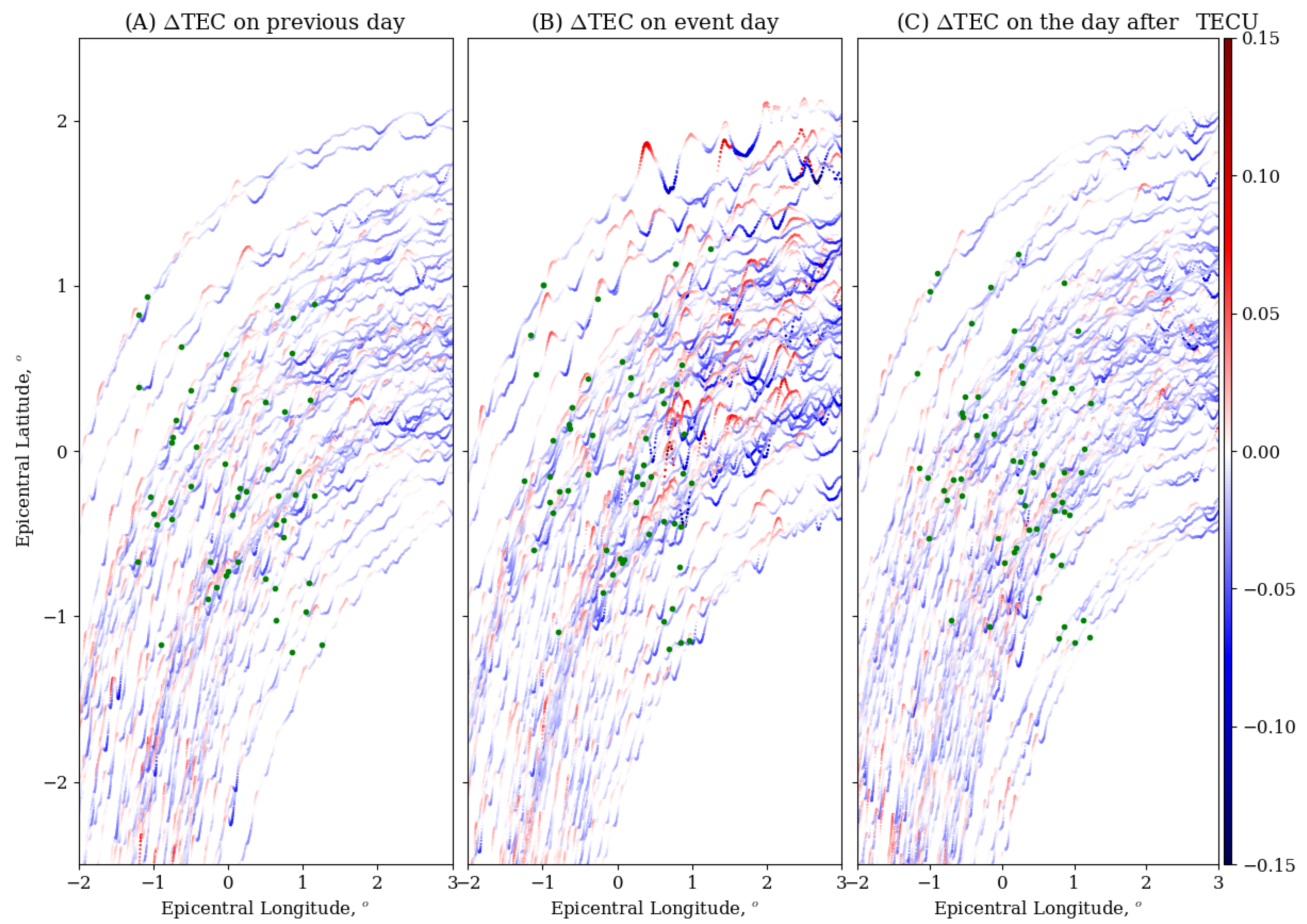
2.3. Estimations of TEC and TEC Disturbance (ΔTEC)

The TEC is estimated from the phase and code measurements from ground-based GNSS-receivers (e.g., Hofmann-Wellenhof et al. [32]), based on the following equation,

$$\mathrm{TEC}=\frac{1}{40.308}\frac{f_1^2{f}_2^2}{f_1^2-f_2^2}(L_1{\lambda }_1-L_2{\lambda }_2+const+nL),$$

(1)

where $f_1$ = 1575.42 MHz and $f_2$ = 1227.60 MHz are carrier-wave frequencies, ${\lambda }_1=c/f_1$ and ${\lambda }_2=c/f_2$ are the corresponding wavelengths in meters, c is the speed of light, $L_1$ and $L_2$ are the carrier phases, $const$ is the unknown initial phase ambiguity, and $nL$ is the error in determining the phase path. The TEC is measured in TEC units (TECU) with 1 TECU = ${10}^{16} \mathrm{el}/{\mathrm{m}}^2$. The precision of TEC estimation from phase measurements is about 0.01–0.02 TECU [33].

We examined TEC data with elevations higher than 20°. The TEC disturbance, $\Delta$TEC, was obtained by employing the Morlet wavelet [34] at various frequencies in 1–10 mHz, i.e., in the frequency range of the Earth’s normal modes [2]. In addition, the net $\Delta$TEC in frequency range of 1–10 mHz was obtained by taking average of various $\Delta$TEC modes at frequencies between 1 and 10 mHz.

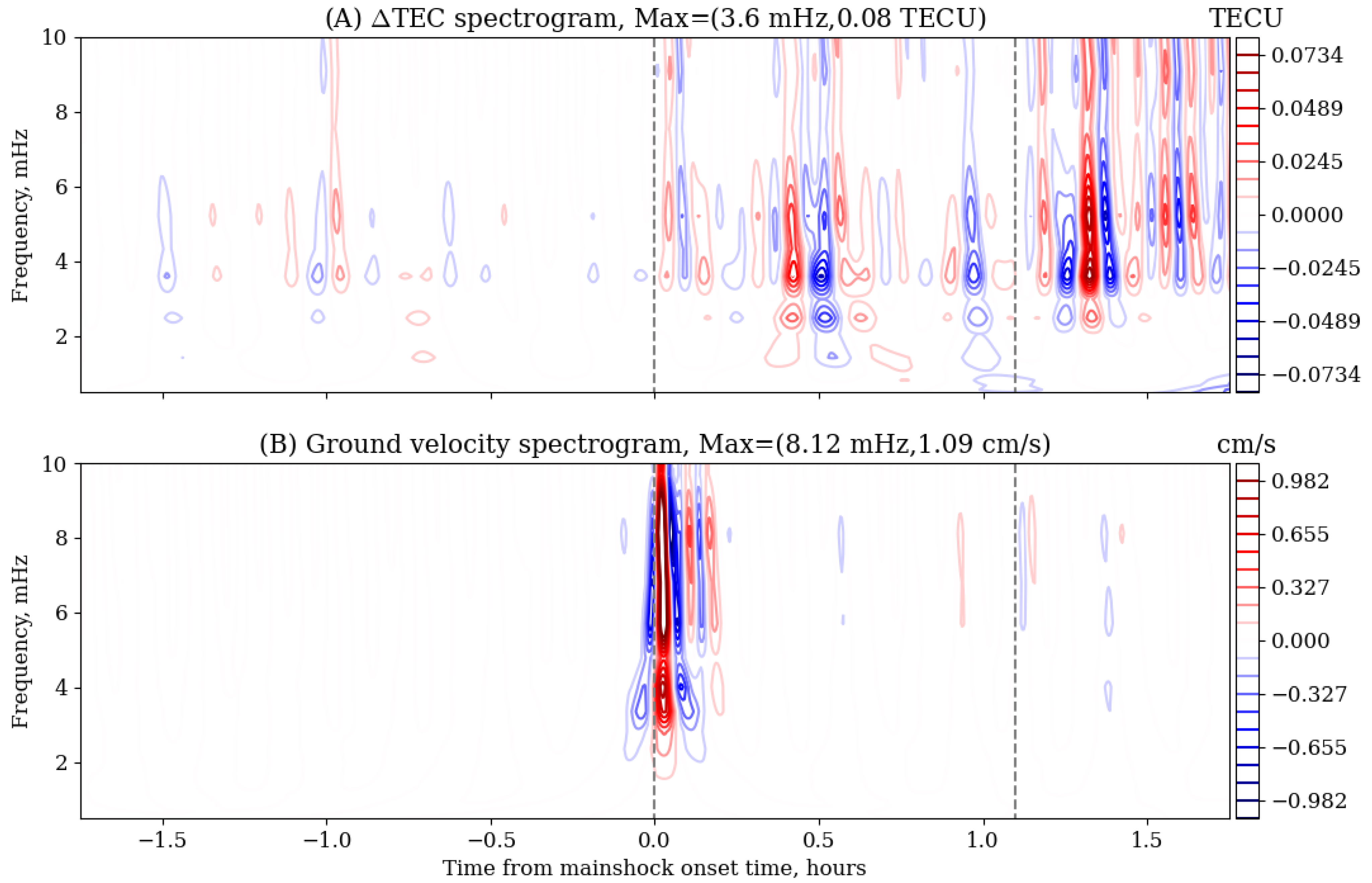
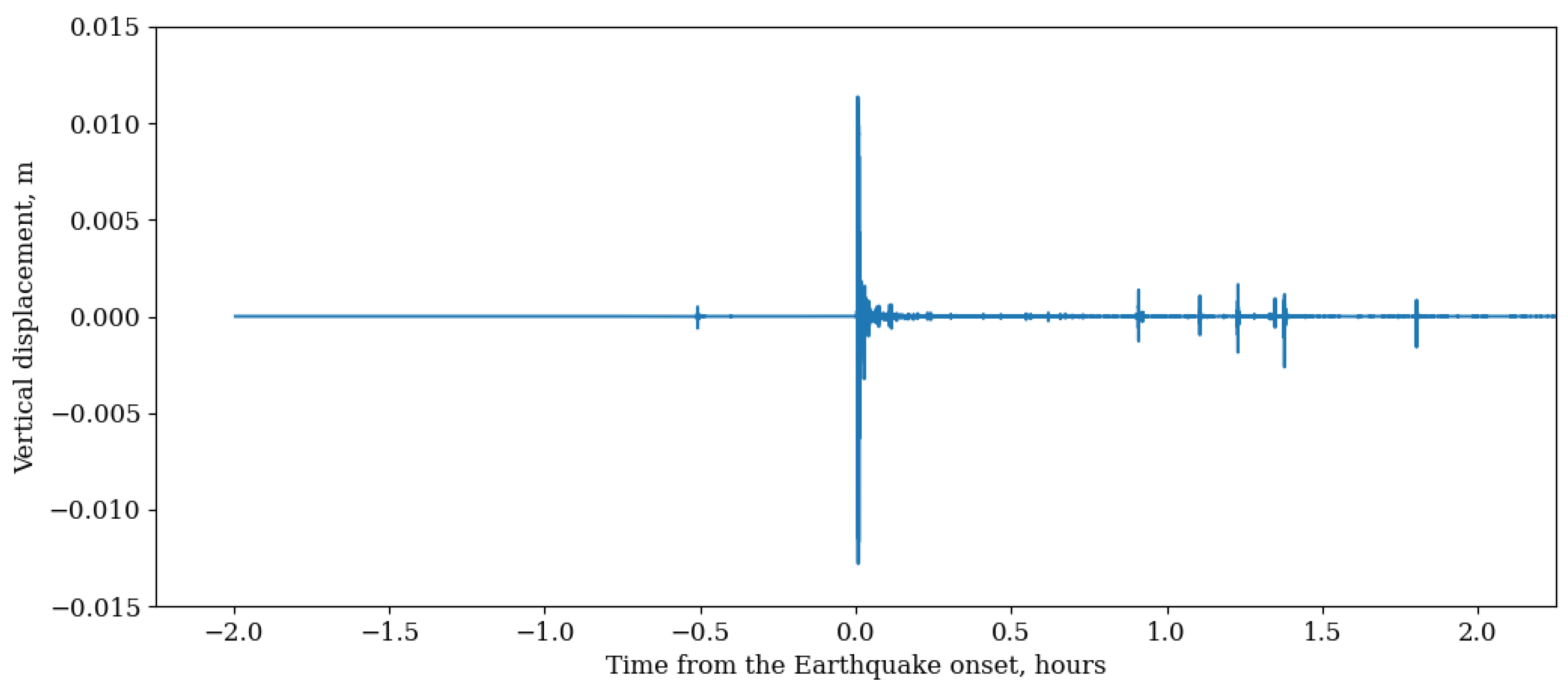
2.4. Estimation of Ground Vertical Velocity and Displacement from Recorded Ground Motion

We employed the ObsPy library of python to process the recorded ground motions (in counts format) from the seismometers around the epicenter [35]. The module downloads the data in counts format and estimates the velocity and displacement of ground motion with the instrumental response corrections that include the removal of frequency response of the seismometers, the effects of any amplifiers, of analog and digital filters, and of the digitalization.

3. Results and Discussion

3.1. Ionoquakes during a Mainshock of $Mw$ 6.4

In Figure 2A, the ground vibration, in the form of vertical velocity (V${}_{\mathrm{SISM}}$, cm/s), is plotted. It reveals the mainshock onset at 17.56 UT and a series of aftershocks; the largest occurred at 18.66 UT (indicated by the dashed line). Interestingly, despite the strike-slip focal mechanism, the mainshock attained a peak velocity of 6 cm/s, which is larger than the mainshock amplitudes at far-field stations of many dip-slip EQs that produced ionoquakes, as investigated by Artru et al. [2]. Artru et al. [2] also demonstrated that the Earth’s normal modes in the frequency range of 1–10 mHz were responsible for the ionoquakes associated with the 1999 Chi-Chi earthquake.

Figure 2B shows the TEC along the trajectory of PRN19 as registered by various GNSS stations. It reveals the availability of continuous TEC data in ±2.25 h from the main shock onset time (17.56 UT) so that the ionospheric variations are monitored well in advance. This time window is adequate for monitoring the dynamics of TEC disturbances generated from both seismic and non-seismic sources around the epicenter. This wide time window permits the spectral analysis to resolve the frequencies higher than 1 mHz so that the TEC data in ±2.25 h remain unaffected by the edge effects arising from the filtering and running mean average processes employed in the study.

Figure 3 shows the temporal variations in $\Delta$TEC in space around the epicenter. Figure 3B reveals the surge in intensified wave oscillations after the mainshock onset on earthquake day, but no such surge can be noted in Figure 3A,C on the previous day or on the day after, respectively. Therefore, from this spatio-temporal analysis, we concluded that the intensified TEC disturbances in Figure 3B were likely of seismic origin.

We note that the amplitude of the intensified $\Delta$TEC variations was about ±0.15 TECU, i.e., more than 10 times exceeding the accuracy of GNSS-TEC of 0.01–0.02 TECU (e.g., Coster et al. [33]).

In addition, we analyzed the spectral characteristics of $\Delta$TEC (Figure 4A). We note that the oscillations intensified ∼30 min after the mainshock onset. This timing suggests the seismic-origin nature of the intensified $\Delta$TEC disturbances, as also shown in Figure 3B. Notably, the intensification concentrated in the 1–6 mHz frequency range i.e., in the acoustic-gravity wave modes in which efficient seismic–ionospheric coupling has ben previously reported [2,19]. The spectral evolution of $\Delta$TEC is similar to that presented by Rolland et al. [19] for various strong EQs. Moreover, we note from the ground velocity spectrogram in Figure 4B that the mainshock velocity in the 1–6 mHz band was about 0.05–0.6 cm/s, which is much larger than the 0.01 cm/s measured over France following the 1999 Chi-Chi earthquake [2]. Therefore, the intensified $\Delta$TEC oscillations prior to the onset of the series of aftershocks in Figure 4A should be a part of ionoquakes in the form of gravity waves generated by the mainshock of magnitude 6.4.

To examine the wave nature and propagation characteristics of $\Delta$TEC oscillations, we plotted the travel–time diagram, or hodogram, from the temporal and latitudinal distribution of $\Delta$TEC. Figure 5, Figure 6 and Figure 7 present the hodograms constructed around the epicenter from about 400 trajectories on the earthquake day (Figure 6), previous day (Figure 5), and day after (Figure 7). On earthquake day, we note two distinct characteristics: (1) the intensification of $\Delta$TEC after the onset time of the mainshock, and (2) emergence of southward-propagating wavefronts (marked as two ellipses) in the vicinity of the epicenter during 0.5–1 h from the mainshock onset. These two characteristics were absent on the pre- and post-EQ days. Therefore, we concluded that on the day of the earthquake, ionoquakes were generated in the form of amplified $\Delta$TEC and southward-propagating wavefronts in the vicinity of the epicenter.

3.2. Solar and Geomagnetic Activity during the Ionoquakes

It is known that enhanced solar and geomagnetic activities are the primary sources of disturbances in the ionosphere and thermosphere (e.g., [36,37]). During the observation of ionoquakes, the planetary Kp index varies between 2 and 2+ (according to the World Data Center in Kyoto, http://wdc.kugi.kyoto-u.ac.jp/ (accessed on 5 November 2021)), which indicates a low level of geomagnetic activity. Further analysis revealed that the solar wind speed was around 340 km/s, and no strong fluctuations were observed (Figure A4 in Appendix A). The interplanetary magnetic field north–south component (IMF Bz) fluctuated between $\pm 4$ nT. The SYM-H index was positive and below +10 nT. Another index, the auroral electrojet (AE), showed a small increase up to 400–500 nT several hours before the earthquake (http://wdc.kugi.kyoto-u.ac.jp/ae_realtime/201907/index_20190704.html (accessed on 5 November 2021); Figure A4d in Appendix A). Therefore, the activity can be characterized as low to low-moderate. The enhanced auroral activity can generate Pc3–Pc5 and omega-band (Ps6) pulsations, but also TIDs of different wavelengths [9,38]. Such disturbances be detected global-wide and do not have any correlation with the epicenter. In our case, however, Figure 6 clearly shows that the ionoquakes were generated around the epicentral area and propagated southward.

3.3. Ionoquakes and Co-Seismic Crustal Displacements

Artru et al. [2] reported observations of ionoquakes associated with the seismic surface wave following the 1999 Chi-Chi EQ epicenter (lat, lon: 23.772°, 120.82°) registered by the Francourville sounding station (lat, lon: 48.39°, 1.63°), France, i.e., ∼9976 km away from the epicenter. They showed that the vertical ground velocity of the order of 0.001 cm/s can drive an ionospheric drift of 0.6 m/s, consistent with the ionospheric Doppler sounding measurements they recorded over France. Figure 4B shows the mainshock ground vertical velocity at 2–6 mHz is about 0.1–0.6 cm/s and, therefore, the corresponding ionospheric drift is about 60–360 m/s. In acoustic-gravity wave mode frequencies of 2–6 mHz, these drifts are sufficient to uplift–downlift the ionosphere by more than a scale height and can generate disturbances detectable in GNSS-TEC measurements, as we found in the present study. Therefore, even though the present event is a moderate EQ, the seismic energy transferred in the normal modes was sufficient to generate ionoquakes in TEC.

According to Cahyadi and Heki [29], only EQs with a ground displacement larger than 0.3 m generate detectable ionoquakes in TEC measurements. The ground displacement derived from the seismometer data attained a mainshock uplift of about 0.013 m (Figure A2 in Appendix A). Additinoally, Liu et al. [39], using GPS data, showed that the co-seismic vertical ground displacement due to the mainshock of the Ridgecrest earthquake reached approximately 0.02 m. These values are well below the threshold value of 0.3 m found by Cahyadi and Heki [29]. The mainshock ground vertical velocity of 0.5 cm/s at 5.0 mHz in Figure 4B corresponds to an uplift of about 1.0 m. In the 2–6 mHz frequency range that hosts most of the ionoquakes, the ground velocity is in the range of 0.1–0.6 cm/s, which corresponds to a ground uplift of 0.5–1.0 m. Therefore, the mainshock satisfies the threshold condition and, hence, the EQ of $\mathrm{Mw}$ 6.4 can generate the seismic-origin disturbances identified in the hodogram in Figure 6. This also implies that the ground velocity of normal modes might be the factor that determines the amplitude of ionoquakes. In addition, significant horizontal displacements occurring beneath areas with high topography can reinforce the vertical component.

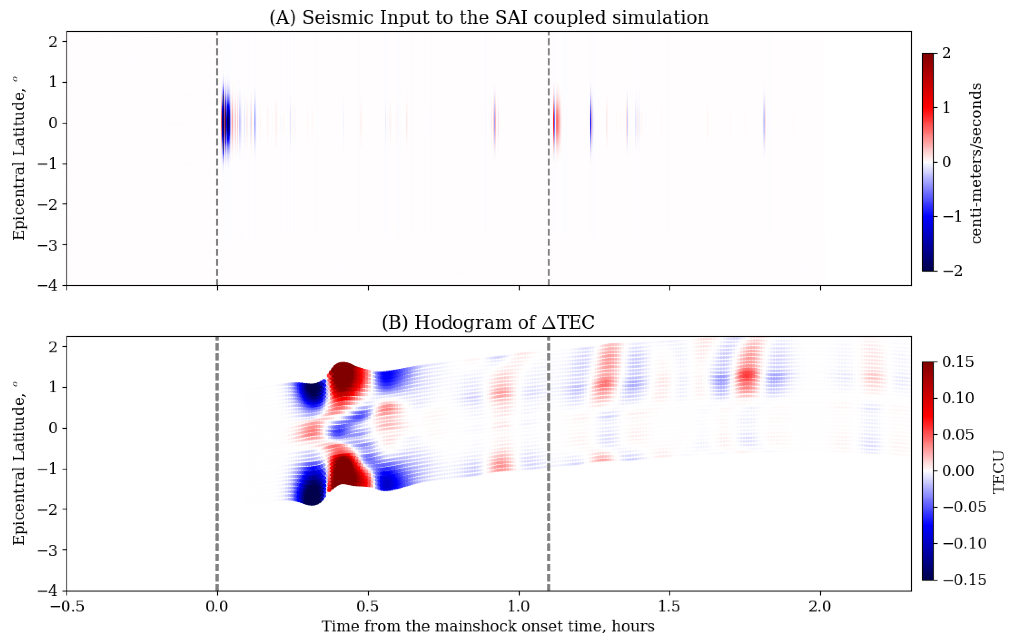
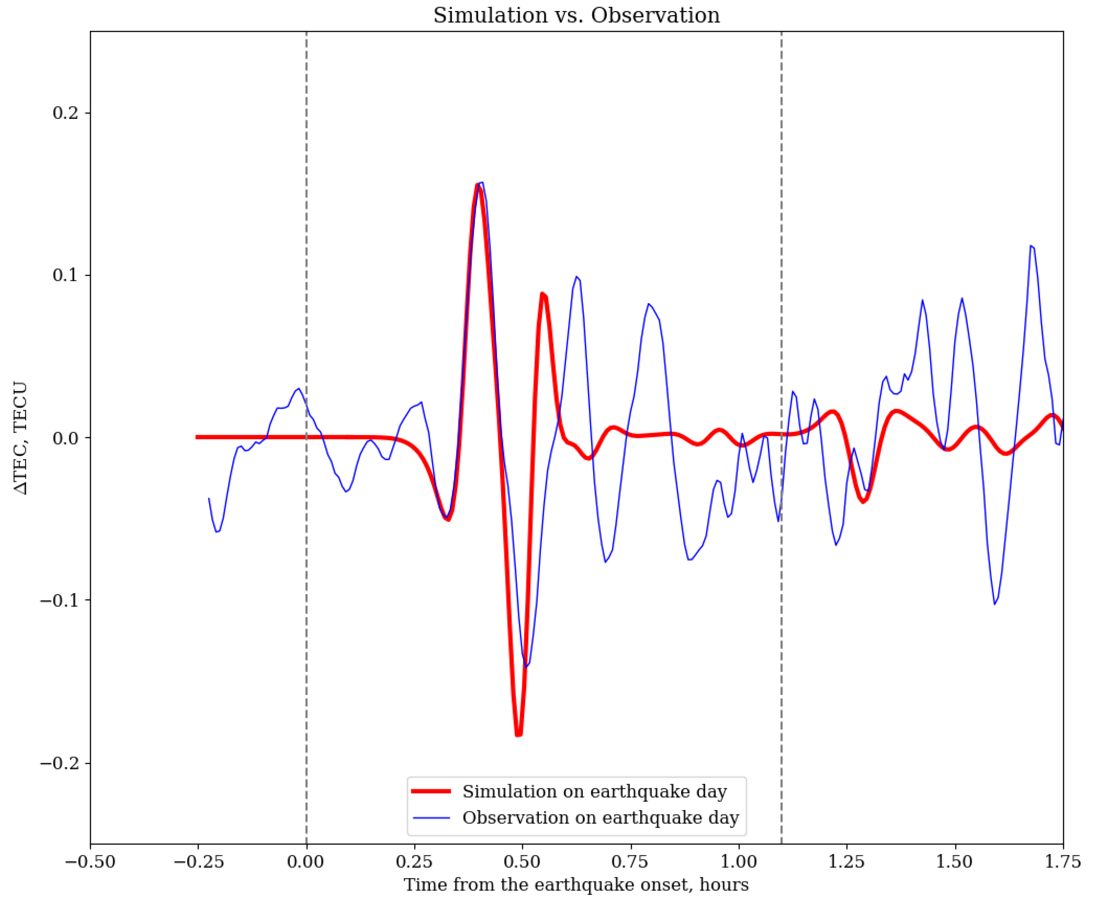
3.4. Ionoquake Simulation

The dominant presence of acoustic and gravity modes in Figure 4 suggests the participation of acoustic gravity waves (AGWs) in the coupling mechanism between the ground and ionosphere [5,19]. This seismo–atmosphere–ionosphere (SAI) coupling mechanism is robust since it uniquely explains the detectable $\Delta$TEC arising from the tiny ground uplift as low as 0.01 m due to the amplification by 3–4 orders at ionospheric heights [7,16]. In the present study, we employed the SAI coupling simulation model [40] that, in the past, was used to simulate the ionoquakes from tsunamis. In the present study, instead of a tsunami wave, the forcing from the ground vibration in the form of vertical velocity was considered. Figure 8A illustrates the real seismic forcing in time and latitude, composed of a mainshock onset at t = 0 min and a series of aftershocks similar to the seismometer-deduced ground velocity (Figure 2A). Only the 1–10 mHz bandpass-filtered ground velocity from the seismometer was considered to reconstruct the ground forcing in the simulation. Based on the shakemap of the mainshock in Figure A1 (Appendix A), the horizontal Gaussian width of the forcing is considered to be 1°. The forcing launches AGWs in the atmosphere that subsequently generates the ionospheric disturbances. Figure 8B presents the hodogram of the simulated $\Delta$TEC, revealing the generation of wavefronts caused by acoustic waves propagating outward from the epicenter within 10 min from the mainshock onset. In particular, the simulated hodogram reveals two southward-propagating wavefronts during 0.5–1 h in 0–$-2^{\circ }$ epicentral latitudes, similar to those marked by ellipses in Figure 6. In addition, it reveals the generation of ionoquakes with an amplitude of about 0.05 TECU during the series of aftershocks, a clear demonstration of positive feedback from the aftershocks of magnitudes $\mathrm{Mw}$ of 4.6. Figure A3 (Appendix A) presents the simulated $\Delta$TEC with and without aftershocks. We note that the mainshock alone does not produce ionoquakes one hour after the mainshock onset. Therefore, the simulated ionoquakes during the aftershock in Figure 8B are mainly associated with the aftershocks.

Figure 9 presents a comparison between the simulated and observed $\Delta$TEC along the IPP trajectories, as registered from the BGIS station. Similar to the observation, the simulated $\Delta$TEC reveals a surge of ionoquakes after the mainshock. The ionoquakes produced from the mainshock during 0.25–0.75 h have a similar waveform and amplitude as the observed ionoquakes. Therefore, the SAI coupling mechanism triggered by the ground velocity and energized by AGWs is one of the possible generation mechanisms for the observed ionoquakes.

We also note disagreement in the observed and simulated waveforms after 0.75 h. The difference is attributed to the following factors: non-seismic contributions to the observed waveform that are absent in the simulation, the seismic forcing considered in the simulation that is not identical to the original shakemap in regards to the spatial distribution, and the ambient atmospheric and ionospheric conditions of the simulation being not identical to the original ambient conditions.

In the excitation of AGWs, the ground velocity, rather than the ground displacement, plays the determining role because the product of these waves is the atmospheric wind disturbance [41] responsible for the ionospheric current and TEC disturbances. Therefore, in the SAI coupling mechanism that satisfactorily simulated the ionoquake, the ground velocity determines the formation of TEC disturbances.

The foreshocks of strong EQs are a series of small and moderate EQs that occur several hours before a strong EQ during the nucleation of rupture [42]. The present study’s findings showed that even the ionoquakes associated with a moderate EQ of $\mathrm{Mw}$ 6.4 can be detected. Moreover, the simulation revealed that the small EQs, in the form of a series of aftershocks of magnitudes ≤4.6, also register contribution to the ionoquakes. Therefore, together with the ground observation, ionospheric seismology offers a promising scenario for the possible short-term forecasting of strong EQs for which no reliable criteria are available to distinguish foreshocks from the EQs alone from the ground measurements. We note that our findings reveald the contribution of aftershocks only with the implementation of simulation of the SAI coupling mechanism. Therefore, the tools and methodology adopted in this study are productive. Their performance can be evaluated for other small and moderate EQs events.

4. Summary

We reported the ionospheric disturbances associated with the 4 July 2019 Ridgecrest earthquake of $\mathrm{Mw}$ 6.4. The GNSS-TEC measurements registered these ionoquakes as intensified wave activities in the range of 1–10 mHz after the mainshock onset and in the vicinity of the epicenter, in contrast to the weak and irresolute wave activities on the pre-earthquake day (3 July 2019) and post-earthquake day (5 July 2019). Based on the seismo–atmosphere–ionosphere (SAI) coupling mechanism energized by the acoustic-gravity waves, we finfoundd that the ground vibration of 0.05–0.6 cm/s in the normal mode frequencies was adequate to produce detectable ionoquakes with an amplitude of about 0.05–0.15 TECU. Our major finding is that the ground velocity, rather than the ground displacement, satisfies the threshold criterion for the formation of detectable ionoquakes. Therefore, though the mainshock was moderate in nature, the associated ground velocity in low-frequency acoustic-gravity modes is comparable to those from the mainshock of strong earthquakes. Further investigations are necessary to obtain robust results.

The numerical simulation of the coupling mechanism not only reproduced the ionoquakes of detectable magnitudes associated with the mainshock but also quantified the relative contribution of the mainshock and aftershocks. Interestingly, the simulated ionoquakes from the aftershock had a magnitude of 0.01 TECU, which is well below the detectable limit of GNSS-TEC measurements. Nevertheless, the simulation of the ionospheric counterpart of aftershocks demonstrated the robust nature of SAI coupling to facilitate the generation of ionoquakes from the small EQs. This work is among few to report the detection and simulation of ionoquakes from a $\mathrm{Mw}$ 6.4 earthquake. Additionally, we are the first to report the simulation of ionoquakes of about 0.05 TECU amplitudes from a series of aftershocks of magnitude $\mathrm{Mw}$ 4.6.

References

1. Calais, E.; Minster, J.B. GPS, earthquakes, the ionosphere, and the Space Shuttle. Phys. Earth Planet. Inter. 1998, 105, 167–181. [Google Scholar] [CrossRef]
2. Artru, J.; Farges, T.; Lognonné, P. Acoustic waves generated from seismic surface waves: Propagation properties determined from Doppler sounding observations and normal-mode modelling. Geophys. J. Int. 2004, 158, 1067–1077. [Google Scholar] [CrossRef]
3. Heki, K.; Ping, J. Directivity and apparent velocity of the coseismic ionospheric disturbances observed with a dense GPS array. Earth Planet. Sci. Lett. 2005, 236, 845–855. [Google Scholar] [CrossRef] [Green Version]
4. Liu, J.Y.; Tsai, Y.B.; Chen, S.W.; Lee, C.P.; Chen, Y.C.; Yen, H.Y.; Chang, W.Y.; Liu, C. Giant ionospheric disturbances excited by the M9.3 Sumatra earthquake of 26 December 2004. Geophys. Res. Lett. 2006, 23, L02103. [Google Scholar] [CrossRef] [Green Version]
5. Lognonné, P. Seismic waves from atmospheric sources and atmospheric/ionospheric signatures of seismic waves. In Infrasound Monitoring for Atmospheric Studies; Springer: Berlin/Heidelberg, Germany, 2009; pp. 281–308. [Google Scholar]
6. Astafyeva, E.; Heki, K. Two-mode long-distance propagation of coseismic ionosphere disturbances. J. Geophys. Res. Space Phys. 2009, 114, A10. [Google Scholar] [CrossRef] [Green Version]
7. Chum, J.; Hruska, F.; Zednik, J.; Lastovicka, J. Ionospheric disturbances (infrasound waves) over the Czech Republic excited by the 2011 Tohoku earthquake. J. Geophys. Res. Space Phys. 2012, 117, A8. [Google Scholar] [CrossRef] [Green Version]
8. Occhipinti, G.; Rolland, L.; Lognonné, P.; Watada, S. From Sumatra 2004 to Tohoku-Oki 2011: The systematic GPS detection of the ionospheric signature induced by tsunamigenic earthquakes. J. Geophys. Res. Space Phys. 2013, 118, 3626–3636. [Google Scholar] [CrossRef]
9. Afraimovich, E.L.; Astafyeva, E.I.; Demyanov, V.V.; Edemskiy, I.K.; Gavrilyuk, N.S.; Ishin, A.B.; Kosogorov, A.B.; Leonovich, E.A.; Lesyuta, L.A.; Lesyuta, O.S.; et al. A review of GPS/GLONASS studies of the ionospheric response to natural and anthropogenic processes and phenomena. J. Space Weather Space Clim. 2013, 3, A27. [Google Scholar] [CrossRef] [Green Version]
10. Astafyeva, E. Ionospheric detection of natural hazards. Rev. Geophys. 2019, 57, 1265–1288. [Google Scholar] [CrossRef]
11. Meng, X.; Vergados, P.; Komjathy, A.; Verkhoglyadova, O. Upper atmospheric responses to surface disturbances: An observational perspective. Radio Sci. 2019, 54, 1076–1098. [Google Scholar] [CrossRef] [Green Version]
12. Heki, K. Ionospheric disturbances related to earthquakes. In Ionosphere Dynamics and Applications; Huang, C., Lu, G., Zhang, Y., Paxton, L.J., Eds.; American Geophysical Union: Hoboken, NJ, USA, 2021; pp. 511–526. [Google Scholar] [CrossRef]
13. Nayak, S.; Bagiya, M.S.; Maurya, S.; Hazarika, N.K.; Kumar, A.S.S.; Prasad, D.S.V.V.D.; Ramesh, D.S. Terrestrial resonant oscillations during the 11 April 2012 Sumatra doublet earthquake. J. Geophys. Res. Space Phys. 2021, e2021JA029169. [Google Scholar] [CrossRef]
14. Kherani, E.A.; Abdu, M.A.; de Paula, E.R.; Fritts, D.C.; Sobral, J.H.; de Meneses, F.C., Jr. The impact of gravity waves rising from convection in the lower atmosphere on the generation and nonlinear evolution of equatorial bubble. Ann. Geophys. 2009, 27, 657–1668. [Google Scholar]
15. Chum, J.; Liu, J.Y.; Laštovička, J.; Fišer, J.; Mošna, Z.; Baše, J.; Sun, Y.Y. Ionospheric signatures of the 25 April 2015 Nepal earthquake and the relative role of compression and advection for Doppler sounding of infrasound in the ionosphere. Earth Planets Space 2016, 68, 1–12. [Google Scholar] [CrossRef] [Green Version]
16. Ducic, V.; Artru, J.; Philippe, L. Ionospheric remote sensing of the Denali Earthquake Rayleigh surface waves. Geophys. Res. Lett. 2003, 30, 1952. [Google Scholar] [CrossRef]
17. Astafyeva, E.; Heki, K. Dependence of waveform of near-field coseismic ionospheric disturbances on focal mechanisms. Earth Planets Space 2009, 61, 939–943. [Google Scholar] [CrossRef] [Green Version]
18. Liu, J.Y.; Tsai, H.F.; Lin, C.H.; Kamogawa, M.; Chen, Y.I.; Lin, C.H.; Huang, B.S.; Yu, S.B.; Yeh, Y.H. Coseismic ionospheric disturbances triggered by the Chi-Chi earthquake. J. Geophys. Res. Space Phys. 2010, 115, A08303. [Google Scholar] [CrossRef]
19. Rolland, L.M.; Lognonné, P.; Astafyeva, E.; Kherani, E.A.; Kobayashi, N.; Mann, M.; Munekane, H. The resonant response of the ionosphere imaged after the 2011 off the Pacific coast of Tohoku Earthquake. Earth Planets Space 2011, 63, 62. [Google Scholar] [CrossRef] [Green Version]
20. Komjathy, A.; Galvan, D.A.; Stephens, P.; Butala, M.D.; Akopian, V.; Wilson, B.; Verkhoglyadova, O.; Mannucci, A.J.; Hickey, M. Detecting ionospheric TEC perturbations caused by natural hazards using a global network of GPS receivers: The Tohoku case study. Earth Planets Space 2012, 64, 1287–1294. [Google Scholar] [CrossRef] [Green Version]
21. Komjathy, A.; Yang, Y.M.; Meng, X.; Verkhoglyadova, O.; Mannucci, A.J.; Langley, R.B. Review and perspectives: Understanding natural-hazards-generated ionospheric perturbations using GPS measurements and coupled modeling. Radio Sci. 2016, 51, 951–961. [Google Scholar] [CrossRef]
22. Bagiya, M.S.; Sunil, P.S.; Sunil, A.S.; Ramesh, D.S. Coseismic Contortion and Coupled Nocturnal Ionospheric Perturbations During 2016 Kaikoura, Mw 7.8 New Zealand Earthquake. J. Geophys. Res. Space Phys. 2018, 123, 1477–1487. [Google Scholar] [CrossRef]
23. Nguyen, C.T.; Oluwadare, S.T.; Le, N.T.; Alizadeh, M.; Wickert, J.; Schuh, H. Spatial and Temporal Distributions of Ionospheric Irregularities Derived from Regional and Global ROTI Maps. Remote Sens. 2022, 14, 10. [Google Scholar] [CrossRef]
24. Yuan, Y.; Ou, J. Auto-covariance estimation of variable samples (ACEVS) and its application for monitoring random ionospheric disturbances using GPS. J. Geod. 2001, 75, 438–447. [Google Scholar] [CrossRef]
25. Astafyeva, E.; Shults, K. Ionospheric GNSS imagery of seismic source: Possibilities, difficulties, and challenges. J. Geophys. Res. Space Phys. 2019, 124, 534–543. [Google Scholar] [CrossRef] [Green Version]
26. Maletckii, B.; Astafyeva, E. Determining spatio-temporal characteristics of Coseismic Travelling Ionospheric Disturbances (CTID) in near real-time. Sci. Rep. 2021, 11, 20783. [Google Scholar] [CrossRef] [PubMed]
27. Zedek, F.; Rolland, L.M.; Dylan Mikesell, T.; Sladen, A.; Delouis, B.; Twardzik, C.; Coïsson, P. Locating surface deformation induced by earthquakes using GPS, GLONASS and Galileo ionospheric sounding from a single station. Adv. Space Res. 2021, 68, 3403–3416. [Google Scholar] [CrossRef]
28. Perevalova, N.P.; Sankov, V.A.; Astafyeva, E.I.; Zhupityaeva, A.S. Threshold magnitude for ionospheric TEC response to earthquakes. J. Atmos. Sol.-Terr. Phys. 2014, 108, 77–90. [Google Scholar] [CrossRef]
29. Cahyadi, M.N.; Heki, K. Coseismic ionospheric disturbance of the large strike-slip earthquakes in North Sumatra in 2012: Mw dependence of the disturbance amplitudes. Geophys. J. Int. 2015, 200, 116–129. [Google Scholar] [CrossRef] [Green Version]
30. Farges, T.; Artru, J.; Lognonné, P.; Le Pichon, A. Effets des séismes sur l’ionosphère; Chocs, 26; CEA-DAM Île-de-France: Arpajon, France, 2002; pp. 7–18. [Google Scholar]
31. Ross, Z.E.; Idini, B.; Jia, Z.; Stephenson, O.L.; Zhong, M.; Wang, X.; Zhan, Z.; Simons, M.; Fielding, E.J.; Jung, S. Hierarchical interlocked orthogonal faulting in the 2019 Ridgecrest earthquake sequence. Science 2019, 366, 5346–5351. [Google Scholar] [CrossRef] [Green Version]
32. Bernhard, H.-W.; Herbert, L.; Elmar, W. GNSS-Global Navigation Satellite Systems; Springer: Vienna, Austria, 2008. [Google Scholar] [CrossRef] [Green Version]
33. Coster, A.; Williams, J.; Weatherwax, A.; Rideout, W.; Herne, D. Accuracy of GPS total electron content: GPS receiver bias temperature dependence. Radio Sci. 2013, 48, 190–196. [Google Scholar] [CrossRef]
34. Poularikas, A.D. Transforms and Applications Handbook, 3rd ed.; CRC Press: Boca Raton, FL, USA; London, UK; New York, NY, USA, 2010. [Google Scholar] [CrossRef]
35. Krischer, L.; Megies, T.; Barsch, R.; Beyreuther, M.; Lecoc, T.; Caudron, C.; Wassermann, J. ObsPy: A bridge for seismology into the scientific Python ecosystem. Comput. Sci. Discov. 2015, 8, 014003. [Google Scholar] [CrossRef]
36. Astafyeva, E.; Heki, K. Vertical TEC over seismically active region during low solar activity. J. Atm. Solar-Terr. Physics 2011, 73, 1643–1652. [Google Scholar] [CrossRef] [Green Version]
37. Cai, X.; Burns, A.G.; Wang, W.; Qian, L.; Pedatella, N.; Coster, A.; Zhang, S.; Solomon, S.C.; Eastes, R.W.; Daniell, R.E.; et al. Variations in thermosphere composition and ionosphere total electron content under “geomagnetically quiet” conditions at solar-minimum. Geophys. Res. Lett. 2021, 48, 2021GL093300. [Google Scholar] [CrossRef]
38. Anderson, B.J. Statistical studies of Pc 3-5 pulsations and their relevance for possible source mechanisms of ULF waves. Ann. Geophys. 1993, 11, 128–143. [Google Scholar]
39. Liu, C.; Lay, T.; Brodsky, E.E.; Dascher-Cousineau, K.; Xiong, X. Coseismic Rupture Process of the Large 2019 Ridgecrest Earthquakes From Joint Inversion of Geodetic and Seismological Observations. Geophys. Res. Lett. 2019, 46, 11820–11829. [Google Scholar] [CrossRef]
40. Kherani, E.A.; Rolland, L.; Lognonne, P.H.; Sladen, A.; Klausner, V.; de Paula, E.R. Traveling ionospheric disturbances propagating ahead of the Tohoku-Oki tsunami: A case study. Geophys. J. Int. 2016, 204, 148–1158. [Google Scholar] [CrossRef] [Green Version]
41. Kherani, E.A.; Abdu, M.A.; Fritts, D.C.; de Paula, E.R. The acoustic gravity wave induced disturbances in the equatorial Ionosphere. In Aeronomy of the Earth’s Atmosphere and Ionosphere; Springer: Dordrecht, The Netherlands; Heidelberg, Germany; London, UK; New York, NY, USA, 2011; pp. 141–162. [Google Scholar] [CrossRef]
42. Sobolev, G. Seismic Quiescence and Activation; Encyclopedia of Solid Earth Geophysics; Springer: Dordrecht, The Netherlands, 2011; pp. 1178–1184. [Google Scholar]
Figure 1. The IPP trajectories of the GPS satellite PRN19 registered by 600 GNSS receivers. The color code represents an observation time between 14 and 20 UT. The star and squares represent earthquake epicenter and seismic stations, respectively.
Remotesensing 14 00188 g001
Figure 2. (A) Vertical ground velocity at 10 seismic stations located within 1° of the epicentral distance; the inset map shows an amplification around the velocity mainshock. (B) TEC values as registered from various stations (total number = 110) located within a ±1.25° epicentral distance at the mainshock onset time. For seismic station with latitude ( l a t s ) and longitude ( l o n s ), epicentral distance is defined as ( l a t s l a t e p ) 2 + ( l o n s l o n e p ) 2 . For GPS trajectories, it is defined as ( l a t 0 l a t e p ) 2 + ( l o n 0 l o n e p ) 2 , where ( l a t 0 , l o n 0 ) are the latitude and longitude of the IPP trajectory at the onset time of the mainshock. Here, ( l a t e p , l o n e p ) is the epicenter coordinate. Vertical dashed lines indicate the onset time of the mainshock of Mw 6.4 and the largest aftershock of Mw 4.6.
Remotesensing 14 00188 g002
Figure 3. TEC disturbance ( Δ TEC) along the IPP trajectories (trajectories are from left to right) in the vicinity of the epicenter on the previous day on 3 July (A), on the event day on 4 July (B), and on the day after on 5 July 2019 (C). The disturbances were extracted from the raw TEC data by applying a bandpass moving average filter with a parameter of 1–10 mHz. Small circles represent the locations of the IPP at the mainshock time. The epicentral latitude and longitude are defined as l a t l a t e p and l o n l o n e p , respectively.
Remotesensing 14 00188 g003
Figure 4. Spectrograms of the Δ TEC (A) and the vertical ground velocity (B) on earthquake day (4 July 2019). Here, TEC and velocities are the averages over all the stations. Red and blue contours represent the positive and negative values, respetively, with the corresponding maximum values denoted as Max at the top of the panel. These maximum values belong to the 1–10 mHz frequency range. Vertical dashed lines indicate the onset time of the mainshock of Mw 6.4 and the aftershock of Mw 4.6. The time window of the data is ±2.25 h; therefore, in 1–10 mHz, the data in ±1.75 h remain unperturbed from the boundary effects arising from the filtering. For this reason, the time axis in this figure and in the rest of the figures is restricted to ±1.75.
Remotesensing 14 00188 g004
Figure 5. Hodogram of the observed Δ TEC on the previous day.
Remotesensing 14 00188 g005
Figure 6. Hodogram of observed Δ TEC on the earthquake day.
Remotesensing 14 00188 g006
Figure 7. Hodogram of observed Δ TEC on the day after the EQ.
Remotesensing 14 00188 g007
Figure 8. Simulation results from the SAI coupling model: (A) the ground vibration at the epicenter, composed of a mainshock at t = 0.0 and a series of aftershocks.(B) A hodogram of the simulated Δ TEC. The hodogram was constructed by estimating the simulated Δ TEC along the IPP trajectories of the hodogram in Figure 6.
Remotesensing 14 00188 g008
Figure 9. Comparison of simulation and observation results for the IPP trajectory, as registered from the BGIS station: simulated and observed Δ TEC of the earthquake day.
Remotesensing 14 00188 g009