Article

Optimization and Evaluation of SO2 Emissions Based on WRF-Chem and 3DVAR Data Assimilation

1
Collaborative Innovation Center on Forecast and Evaluation of Meteorological Disasters (CIC-FEMD), Key Laboratory for Aerosol-Cloud-Precipitation of China Meteorological Administration, Nanjing University of Information Science & Technology, Nanjing 210044, China
2
College of Meteorology and Oceanography, National University of Defense Technology, Changsha 410073, China
3
Institute of Urban Meteorology, China Meteorological Administration, Beijing 100089, China
4
No. 32145 Unit of PLA, Xinxiang 453000, China
*
Author to whom correspondence should be addressed.
Submission received: 23 September 2021 / Revised: 13 December 2021 / Accepted: 28 December 2021 / Published: 4 January 2022

Abstract

:
Emission inventories are important for modeling studies and policy-making, but the traditional “bottom-up” emission inventories are often outdated with a time lag, mainly due to the lack of accurate and timely statistics. In this study, we developed a “top-down” approach to optimize the emission inventory of sulfur dioxide (SO2) using the Weather Research and Forecasting model coupled with Chemistry (WRF-Chem) and a three-dimensional variational (3DVAR) system. The observed hourly surface SO2 concentrations from the China National Environmental Monitoring Center were assimilated and used to estimate the gridded concentration forecast errors of WRF-Chem. The concentration forecast errors were then converted to the emission errors by assuming a linear response from SO2 emission to concentration by grids. To eliminate the effects of modelling errors from aspects other than emissions, a strict data-screening process was conducted. Using the Multi-Resolution Emission Inventory for China (MEIC) 2010 as the a priori emission, the emission inventory for October 2015 over Mainland China was optimized. Two forecast experiments were conducted to evaluate the performance of the SO2 forecast by using the a priori (control experiment) and optimized emissions (optimized emission experiment). The results showed that the forecasts with optimized emissions typically outperformed the forecasts with 2010 a priori emissions in terms of the accuracy of the spatial and temporal distributions. Compared with the control experiment, the bias and root-mean-squared error (RMSE) of the optimized emission experiment decreased by 71.2% and 25.9%, and the correlation coefficients increased by 50.0%. The improvements in Southern China were more significant than those in Northern China. For the Sichuan Basin, Yangtze River Delta, and Pearl River Delta, the bias and RMSEs decreased by 76.4–94.2% and 29.0–45.7%, respectively, and the correlation coefficients increased by 23.5–53.4%. This SO2 emission optimization methodology is computationally cost-effective.

1. Introduction

Sulfur dioxide (SO2) is a major air pollutant that contributes to poor air quality. It has a significant impact on the environment and climate [1,2,3]. A major proportion of anthropogenic SO2 emissions come from power plants and industries, accounting for more than 70% of the total SO2 emissions [4]. It is challenging to predict SO2 concentrations using regional air quality models because of many factors. Firstly, the uncertainty of an emission inventory can affect the accuracy of model forecasts [5,6]. Secondly, the concentrations of air pollutants are affected by meteorological conditions (e.g., wind, precipitation), and the uncertainties associated with the physical parameterization scheme could affect the accuracies of SO2 concentration forecasts [7,8,9]. Thirdly, inaccurate chemistry initial conditions (ICs) can reduce the forecast accuracy. It has been acknowledged that improving the accuracy of ICs by data assimilation (DA) is an effective strategy to improve air pollution forecasting [10,11]. In addition, the conversion of SO2 to sulfate has been commonly underestimated in current global and regional models, leading to an overestimation of SO2 concentrations [12,13,14,15]. The conversion of SO2 to sulfate involves various chemical processes, including gas-phase oxidation, aqueous reactions, and heterogeneous reactions, as well as physical parameters (e.g., relative humidity and cloud fraction). Among the aforementioned factors, emission inventory uncertainty is considered to be the primary factor that influences the forecast accuracy of SO2, especially for complex air pollution analyses in China, where there are varying, multi-source emissions [16,17,18,19]. Improving the accuracy of the emission inventory in terms of the total amount of emissions and the spatial–temporal distribution would facilitate accurate air quality predictions.
Generally, the “bottom-up” approach is used to estimate SO2 emissions, which requires statistical information on the activities and emission factors from all possible sources [4,18,20]. It is difficult to obtain an accurate emission estimate associated with the “bottom-up” approach. The accuracy if emission estimation depends on the qualities and uncertainties of the underlying information from the energy activities at the national, provincial, and county levels [21,22,23]. The difference among some global SO2 emission inventories with the “bottom-up” approach is 42% [24]. In China, the emission estimate is usually updated only once every few years, but the SO2 emissions have decreased by about 62% on average from 2010 to 2017 [4]. Thus, it is difficult for the emission estimate to reflect the change of emissions in real time [12]. In addition, most of the “bottom-up” emission estimates are annual/monthly total amounts, which need to be spatially and temporally allocated into hourly grid emissions for air quality model application [14,25,26,27,28,29]. The grid emission estimates could be inaccurate due to the spatial allocation, casting uncertainty on the model forecast. For the temporal allocation of emission inventories in air quality models, some methods evenly distribute the total 24 h emission amount by virtue of experience [30,31,32]. The hourly factor has often been obtained from power plants’ reports, human activity characteristics, and previous studies [31,32,33,34,35].
To reduce the uncertainties of “bottom-up” emission inventories, some data assimilation (DA) systems were developed to optimize the emission inventories by using observations as constraints [36,37,38,39,40,41,42,43,44]. Lee et al. [40] applied the mass balance method to update SO2 emissions with two satellite instruments (SCIAMACHY and OMI). Koukouli et al. [45] updated SO2 emissions monthly from 2005 to 2015, assuming a linear relationship between SO2 emissions and the satellite SO2 column. The result showed that the SO2 emissions decreased by 28% from 2010 to 2015. Fioletov et al. [46] developed a new mass balance method, which considered the SO2 lifetimes, to estimate SO2 emissions from large SO2 sources by the OMI SO2 column. Based on the four-dimensional variational (4DVAR) method and GEOS-Chem adjoint model, several studies developed inverse models to update monthly SO2 emissions. Wang et al. [47,48] developed an inverse model to update monthly SO2 emissions by assimilating the OMI SO2 satellite measurements. Li et al. [49] optimized SO2 emissions based on OMI SO2 data and then quantitively evaluated the improvement of SO2 emissions by different models, suggesting the efficacy of the optimized emission estimate. The ensemble Kalman filter (EnKF) method is one of the most popular methods used to optimize SO2 emissions. Chen et al. [12] used the ensemble square root filter (EnSRF) system to evaluate SO2 emission changes in January from 2010 to 2015. The results showed that the SO2 emissions decreased by 9.9–22.9% in Southern China, while the SO2 emissions increased by 12.7–72.0% in Northern China and Western China. Dai et al. [50] quantitatively estimated the spatial changes of SO2 emissions in China based on the four-dimensional local ensemble transform Kalman filter method (4D-LETKF). It was shown that the SO2 emissions decreased by 49.4% in November from 2010 to 2016 by assimilating surface SO2 observations.
To date, a three-dimensional variational (3DVAR) assimilation algorithm has been commonly used to improve ICs, but has not been used to update emission inventories within the context of improving air quality forecasts. In this study, we attempted to develop a 3DVAR concentrations converted to emissions (3DVAR-CCE) method in order to improve the SO2 emission inventory based on WRF-Chem and a 3DVAR system. The emission inventory for October 2015 over Mainland China was optimized, and the hourly observed surface SO2 concentrations were assimilated. This study period was chosen because the meteorological conditions during this period were relatively stable and there was relatively little precipitation.
The remainder of this paper proceeds as follows. The methodology is described in Section 2, including the WRF-Chem and 3DVAR DA system configurations and the newly designed SO2 emission optimization procedure. The observational data used for evaluating the model and experimental design are also provided. In Section 3, the reliability of the optimized emission estimates is verified by analyzing recent control policies and possible realistic emission changes. The SO2 simulations, using updated emissions, were also verified against observations to show the emission improvement. A discussion and conclusions are presented in Section 4.

2. Data and Methodology

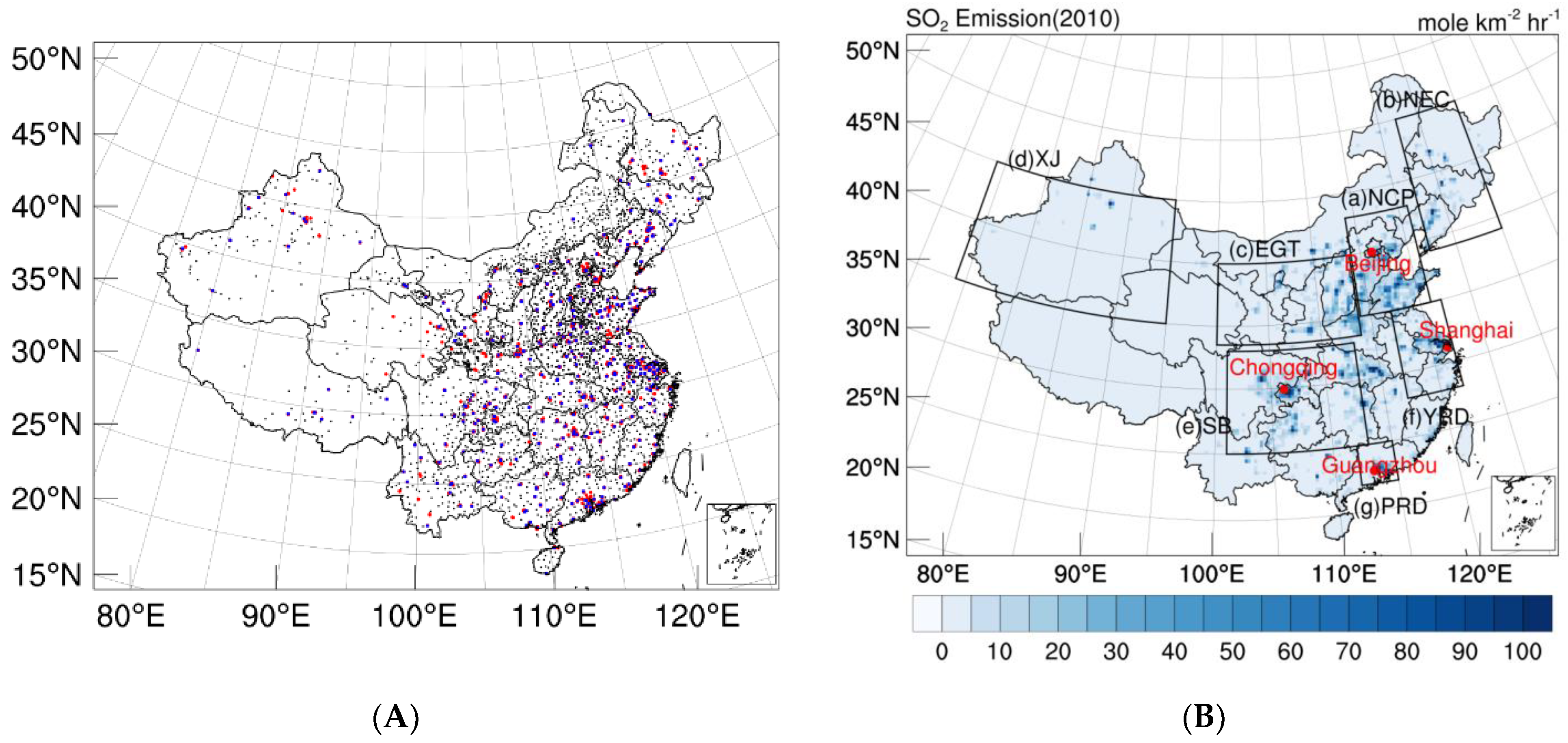
2.1. Observational Data and a Priori Emission Data

Hourly SO2 data from the China National Environmental Monitoring Center (CNEMC) (http://www.cnemc.cn, last access: 23 September 2021) were used for assimilation and evaluation. There were altogether 1497 national control measurement sites over China in 2015. Most observational sites are in Central and Eastern China, whereas the sites in the west are relatively sparse. As shown in Figure 1A, only 1048 stations were selected (randomly) to be assimilated, and the data of the remaining 499 were used to verify the improvement of using optimized emissions. To ensure data quality, the values exceeding 650 µg m−3 were deemed unrealistic and were not assimilated in the 3DVAR system, following Chen et al. [12]. The dataset is widely used to analyze the air quality in China [12,19,21,23,30,42].
Hourly observational data from national automatic meteorological observation stations in China were used in this study. The ground meteorological observation data were collected from the China Meteorological Data Service Centre (http://data.cma.cn/en, last access: 23 September 2021). This dataset is high-quality and widely used in China [52,53]. There were 1623 observational sites in the year 2015. Meteorological variables including surface temperature, relative humidity, precipitation, and wind speed, and direction were included (Figure 1A). The observational data were rigorously quality controlled to reduce the influence of meteorological data outliers on emission optimization by eliminating outliers (e.g., climate extremes) and verifying the temporal and spatial consistencies of the observational data (e.g., wind speed and precipitation data).
A priori emission data from anthropogenic emissions were obtained from the MEIC, developed by Tsinghua University (http://meicmodel.org/?lang=en, last access: 23 September 2021). The resolution is 0.25° × 0.25°, and the base year was 2010. MEIC is a bottom-up emission inventory covering 31 provinces in Mainland China and including eight major chemical species [23]. The MEIC reports anthropogenic emissions from sources in five sectors (power, industry, residential, transportation, and agriculture). The details of the technology-based approach and source classifications can be found in Zhang et al. [23]. The original emission inventory (0.25° × 0.25°) was pre-processed to match the model grid spacing (27 km). Seven different regions are illustrated to address spatial trends, including the North China Plain, Northeast China, Energy Golden Triangle, Xinjiang, Sichuan Basin, Yangzi River Delta, and Pearl River Delta. Figure 1B shows the spatial distribution of a priori SO2 emissions in the simulation domain.

2.2. WRF-Chem Forecast Model and the 3DVAR DA System

The Weather Research and Forecasting (WRF) model coupled with online chemistry (WRF-Chem) Version 3.9.1 was used to simulate and predict air pollutant emissions in this study. The WRF-Chem system is a fully coupled online air quality model that considers several physical and chemical processes, such as transport, deposition, emission, chemical transformation, photolysis, and radiation. The domain (Figure 1) is centered at 101.5° E, 37.5° N and covers all of China, with a 27 km horizontal resolution (169 × 211 grids). There are 40 vertical layers extending from the surface to 50 hPa, with a finer resolution near the surface. Initial and meteorological boundary conditions are provided by the 1° × 1° NCEP Global Final Analysis (FNL) data with a 6 h frequency. The WRF-Chem configuration was set using the physics schemes (Table 1) such as the WRF Lin microphysics scheme [54], the Rapid Radiative Transfer Model longwave [55] and Goddard shortwave radiation schemes [56], the Yonsei University (YSU) boundary layer scheme [57], the Noah land surface model [58], and the Grell-3D cumulus parameterization [59]. The Model for Simulating Aerosol Interactions and Chemistry (MOSAIC-4 bin) and the Carbon Bond Mechanism-Z were chosen for the aerosol and gas-phase chemistry scheme, respectively [60,61]. A nudging scheme was used in the WRF-Chem simulation, and the FNL data were assimilated every 6 h. Anthropogenic emissions from the Multi-Resolution Emission Inventory for China (MEIC) in 2010 were used as the a priori emission input.
The framework of the 3DVAR DA system is very similar to that described by Li et al. [62] and Zang et al. [63,64]. However, previous studies focused on the analysis of ICs for PM2.5 to improve PM2.5 forecasting, and this study focused on the SO2 concentration to improve the emission inventory. The SO2 observations were assimilated using SO2 concentrations as a state variable. The incremental cost function for 3DVAR is as follows:
J ( δ x ) = 1 2 δ x T B 1 δ x + 1 2 ( H δ x d ) T R 1 ( H δ x d )
here, δ x is the N-vector, known as the incremental state variable, which is defined as δ x = x x b , where x b is the forecast or background state of WRF-Chem. B is the N × N -matrix, denoting the background error covariance associated with x b . The M -vector d = y H x b is known as the observation innovation vector, where y is an observation vector, and the M × M -matrix R is the observation error covariance. The H is the observation operator that computes the modeled observation estimates from state variables. With the given observations, the background error covariance (BEC) is also important for determining the performance of a 3DVAR scheme to a substantial degree. In this study, we followed the process outlined by Li et al. [62].
The National Meteorological Center (NMC) method has been used for estimating the air pollutant concentrations’ background error covariance [62,63]. Our previous studies, Li et al. [62] and Zang et al. [63], used 1 mo of the 48 h and 24 h forecast differences as the background error and improved forecasts of PM2.5 concentrations for more than 16 h. The differences between 48 h and 24 h forecasts were generated from 10 October 2015 to November 11 2015. The first initial chemical field at 00 UTC on 10 October 2015 was obtained from a 10 d forecast in consideration of spin-up. The subsequent initial chemical fields were derived from the former forecast one day prior. For a pair of experiments with 24 h and 48 h forecasts, the initial chemical fields were alternatives from different forecasts, resulting in different forecasts for the next cycle. It was assumed that these differences are representative of the short-term forecast errors in transport-related SO2 processes and can be used to calculate the background error covariance of SO2 concentrations [62]. In this study, the forecast differences in SO2 concentrations were used to calculate the BEC.
The horizontal length scale was used to determine the magnitude of SO2 variance in the horizontal direction. This scale can be estimated by the curve of the horizontal correlation with distances, and the horizontal correlation is approximately expressed by a Gaussian function e ( x 1 x ) 2 2 L s 2 . x 1 and x are two points, and L s is the horizontal length scale. According to Zang et al. [63], when the intersection of the decline curve reaches e 1 / 2 , the distance can be approximately as the horizontal length scale in Figure 2a. The horizontal length scale was 81 km, which is approximately three-times larger than the scale used in this study. The vertical variance of SO2 concentrations was considered by vertical correlations in the BEC. A strong relationship was observed in the boundary layer (approximately below the 20th model layer) in the vertical direction (Figure 2b). The standard deviation demonstrates the reliability of the forecasting model, and the standard deviation for the vertical distribution of SO2 concentrations decreased with increasing height in the BEC (Figure 2c).

2.3. The Methodology Used for Optimizing the SO2 Emission Inventory

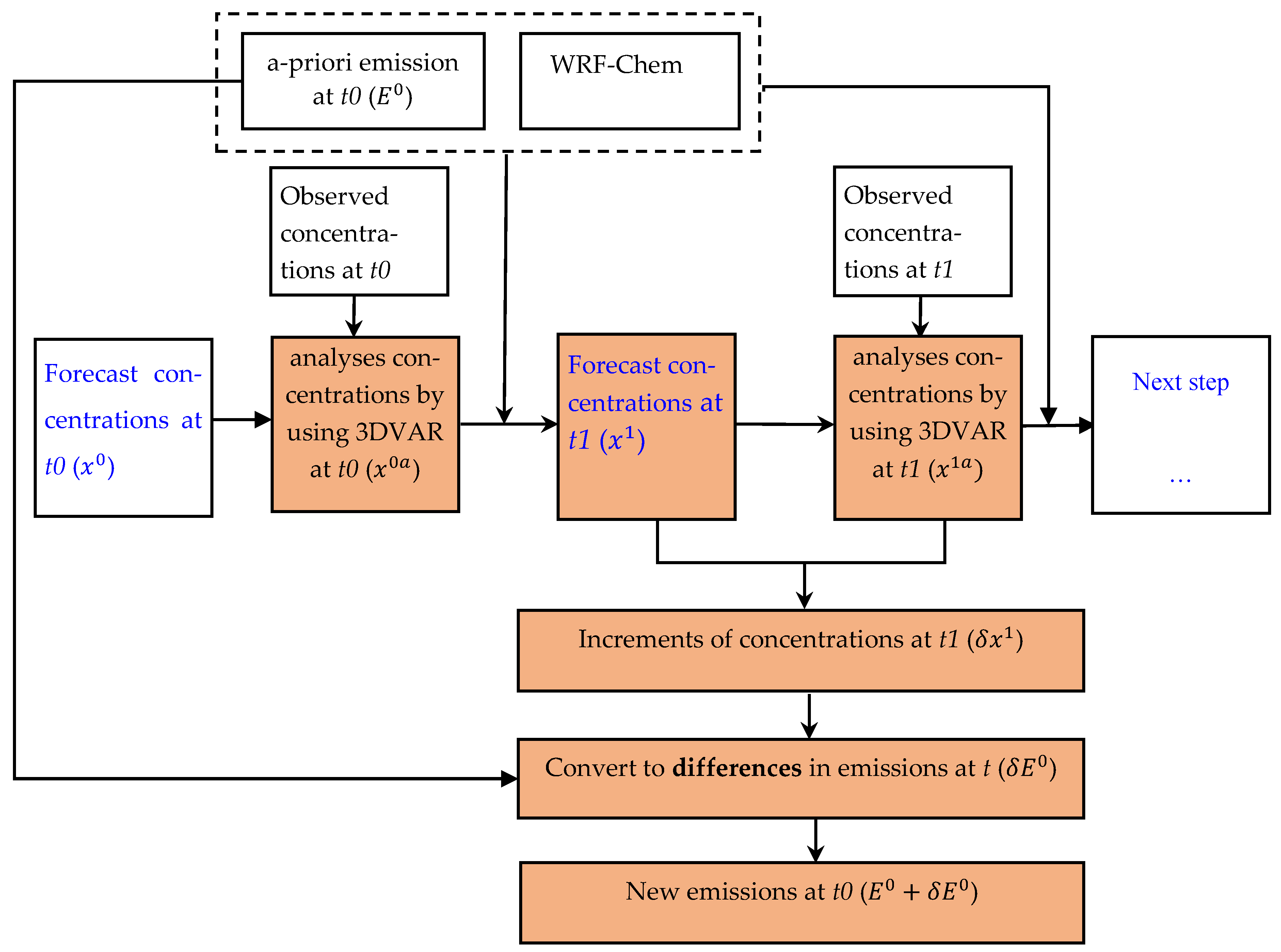
2.3.1. The Assumptions and Procedure to Optimize the Emissions

As stated in the Introduction, forecast errors associated with SO2 simulation concentrations could be induced by many factors, including uncertainties in emission inventories, physical and chemical mechanisms, and ICs. Thus, three important steps to optimize the emissions are to (1) generate the “best” concentration fields to obtain the forecast error, (2) eliminate errors from aspects other than emissions, and (3) convert the concentration forecast error into an emission error. The foremost goal is to generate the best concentration fields by DA because it is the best initial field for forecasting and the increment field for emission optimization.
A flowchart of the procedure for optimizing SO2 emissions for a single time step is shown in Figure 3. First, the background field at time t0 ( x 0 ) was assimilated using 3VDAR with the observation data to obtain the analyzed concentration ( x 0 a ). Second, x 0 was used as the initial field to forecast SO2 at t1 ( x 1 ) using the WRF-Chem model. Third, similar to the first step, the forecasted SO2 concentrations at t1 ( x 1 ), as the background field, were assimilated using 3DVAR with the observation data to obtain the analyzed field ( x 1 a ). Fourth, the difference between x 1 a and x 1 was calculated to represent the forecast error for the SO2 concentrations ( δ x 1 ). Fifth, for each box over a grid area, we assumed that δ x 1 is mainly caused by the emission inventory uncertainty at the former time ( δ E 0 ), that is δ x 1 can be expressed as a function of f ( δ E 0 ) . Some factors contribute to the SO2 forecast error, including the initial field, chemical reactions, and meteorological conditions. The contribution of these factors is relatively small compared with that of the uncertainties in the emission inventory for short-time forecasts (e.g., 1 h), because the initial field is accurate after data assimilation and the chemical reaction error for SO2 is small for the long-life-cycle of SO2. In particular, under the meteorological conditions of clear sky and stationary winds, dry/wet deposition and the diffusion processes are not expected to affect the SO2 forecast error. Sixth, the emission error ( δ E 0 f 1 ( δ x 1 ) ) was calculated by converting the forecast error of the concentration. Finally, the new emission is obtained by adding the emission error ( δ E 0 ) to the prior emission source ( E 0 ).

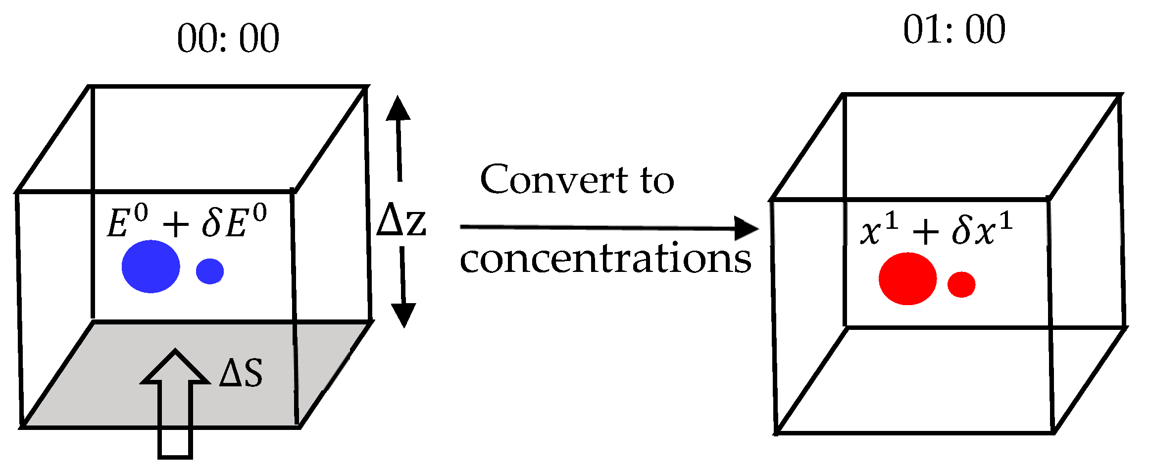
2.3.2. Conversion from Forecast Error to Emission Error

The relationship between the SO2 emission source and the concentrations in a single grid box is shown in Figure 4. It is indicated that the forecast error of the concentrations after 1 h (e.g., 01 UTC) δ x 1 is mainly due to the uncertainty in the emission source 1 h earlier (e.g., 00 UTC) in that grid box. The forecast error of the SO2 concentrations is then converted from the emission flux error using the function below (Figure 3):
δ x 1 f ( δ E 0 ) = V m × ρ a i r ρ × Δ S Δ z × δ E 0 × Δ t
here, V m   ( 22.4 × 10 3   m 3 ) is the gas molar volume, ρ is the air density of the actual atmosphere ( kg   m 3 ), ρ a i r   ( 1.29   kg   m 3 ) is the air density in a standard state indicating the gas molar volume, Δ S is the grid area, Δ z is the mode layer height, and Δ t   ( 1   h ) is the time step. The emission error can be represented by the forecast error for the SO2 concentration in the grid box (Figure 3):
δ E 0 f 1 ( δ x 1 ) = 1 V m × ρ ρ a i r × Δ z Δ S × 1 Δ t × δ x 1
The forecast error of SO2 concentration is defined as δ x 1 = x a 1 x b 1 , where x b 1 is the background of the model forecast after 1 h and x a 1 is the analyzed field obtained by assimilating the observation with the background x b 1 . The x a 1 x b 1 in the assimilation process is also known as the increment field of the SO2 concentration.
δ x 1 is a three-dimensional array, known as the increment field obtained from the background of the model forecast at a 1 h frequency by assimilating the observational data. For each grid, the SO2 increment fields were generated for each hour (00–23 UTC) and then used for emission optimization.

2.3.3. The Operational Consideration for Emission Optimization

To improve the representativeness of δ x 1 at each hour (00–23 UTC), the median value of the SO2 forecast error at each hour in each grid box δ x ( i , j , t ) 1 was obtained from all samples of the SO2 forecast error δ x ( i , j , t , n ) 1 over the entire simulation period (the month of October in this study):
δ x ( i , j , t ) 1 = m i d [ δ x ( i , j , t , n ) 1 , n ]
here, i and j are the grid numbers in the east–west and north–south directions, respectively, and t is the hour of a day. n is the number of simulated days, known as the sample number of that hour, with a maximum of 30 in this study. The median SO2 concentrations’ increment over one month of samples was used to improve the representativeness of the hourly SO2 increment field δ x ( i , j , t ) 1 . Once the median increment field is obtained, the updated emission can also be calculated. δ x ( i , j , t ) 1 in Equation (4) is used to replace δ x 1 in Equation (3):
δ E ( i , j , t ) 0 = 1 V m × ρ ( i , j , t ) ρ a i r × δ z ( i , j ) × 1 δ t × m i d [ δ x ( i , j , t , n ) 1 , n ]
SO2 concentrations are closely related to meteorological conditions [65,66]. Wind can promote the horizontal diffusion of SO2 [67,68] and affect the lifetime of SO2. Fioletov et al. [43] found the correlation between SO2 emissions and SO2 concentrations to be 0.93 when the SO2 life-time was between a few to more than ten hours. In addition, SO2 is converted effectively into sulfate through aqueous reactions in clouds or fog droplets [14], and precipitation affects the wet removal rate of SO2 [69]. To reduce the SO2 forecast error caused by horizontal diffusion, chemical reaction, and wet deposition, we chose only the samples that satisfied several strict conditions to optimize the SO2 emission. Three meteorological variables (precipitation, wind, and divergence) were used as the diagnostic criteria to screen valid samples. The samples with observed hourly precipitation > 0 mm or wind speed > 4 m s−1 were removed to eliminate the effects of wet deposition or heavy diffusion. Since the locations of the observed data are usually not on the model grid, all the samples of the four grids around the observed station were removed. The samples with divergence > 10−4 s−1 were also removed, since SO2 concentrations may diffuse out of the grid box under this condition, resulting in an incorrect estimation. Note that the divergence calculation uses the wind speed of the model grid and not the observed wind speed. Samples with divergence < 0 s−1 were not removed because in this condition, the SO2 concentrations are still in the same box, diffusing upward. The planetary boundary layer height (PBLH) was used to consider the impact of upward diffusion. The SO2 forecast errors for all layers below the PBLH were converted into emission source errors by Equation (3) and then accumulated as the total emission source error.

2.4. Observing Systems Simulation Experiment

An observing systems simulation experiment (OSSE) was designed to evaluate the effect of the inverse model system. The real emission included 273 sources (Figure S1a). These sources were divided into 13 arrays and 9 columns. The data were randomized and placed on the grid as the real emissions. The hourly emission factors of the real emissions were based on industry and power reports. Then, the real emissions and WRF-Chem model were applied to simulate the 10 d SO2 concentrations, and WRF-Chem simulated the “real” SO2 concentrations. The background emission included 273 sources (Figure S1b), which was applied as the a priori emissions. The average value of the background emissions was 50 mol km−2 h−1, and the hour factors of the background emissions were the same.
The OSSE was performed (Figure 5) with the background emissions as the a priori emissions. The hourly real concentrations, which were simulated by using WRF-Chem model with the real emissions, were assimilated to obtain the optimized emissions. The optimized emissions were obtained according to the steps in Figure 3 and Equation (5). In these 10 d DA cycle simulations, approximately 45% of the samples were removed due to precipitation, wind speed, and divergence. Figure 5 shows the scatter plot between real emissions, a priori emissions, and optimized emissions. It was found that the 3DVAR-CCE method could effectively improve the accuracy of the emission source. Compared with the background emissions, the averaged bias and root-mean-squared error (RMSE) were decreased by 4.4 mol km−2 h−1 and 24.3 mol km−2 h−1, respectively, while the correlation coefficient (CORR) increased from 0.2 to 0.9, suggesting that the 3DVAR-CCE method can remarkably improve the SO2 emission source by assimilating the surface SO2 concentration.

2.5. Experimental Design

Three experiments were performed to evaluate the effect of SO2 emission optimization on SO2 concentration forecasts over China, i.e., control experiment, update cycle DA (UC_DA) experiment, and new emission (N_E) experiment, with the simulation period from 10 October 2015 to 10 November 2015. The meteorological conditions during this period were relatively stable, and there was relatively little precipitation. There were more than 10 d with the average wind speed less than 4 m s−1 in 50% of the area of China within 1 mo. For most areas of China, the rainy days were less than 5 d. The emission source from October 10th to November 10th (October, the same as below) was used for emission optimization due to large variations in emission sources (transportation and fireworks) during 1–7 October, coinciding with China’s National Day. The simulated products were produced at hourly intervals. The FNL data with a 6 h frequency were interpolated to a 1 h frequency by running the WRF Pre-processing System (WPS), and the interpolated data were used to update the meteorological IC and boundary conditions (BCs) to prevent meteorology simulation drifting by nudging.
A control experiment was performed without applying DA, initialized with a former forecast result, starting from 00 UTC on October 1 2015, and the emission inventory was MEIC_2010. The UC_DA experiment was started at 00 UTC on October 10 with a 3DVAR analysis field by assimilating the SO2 concentrations and restarted every hour with an updated 3DVAR analysis field as the initial chemical field. For UC_DA experiment, not all observation data were assimilated. In a model grid, if there were more than 2 sites, we randomly selected 1 observation site for verification and other for assimilation purposes. In this study, approximately 1048 national control sites were applied to improve the SO2 ICs, and approximately 449 sites were used to evaluate the model performance (Figure 1A). In the UC_DA experiment, MECI_2010 was used as an a priori emission inventory to simulate the SO2 concentration in October 2015. Then, the updated optimized emissions for 2015 were obtained. To assess the optimized emissions obtained from the UC_DA experiments, an N_EM experiment, starting from 00 UTC on October 10 for the same period, was conducted and the results were compared with those from the control experiment. The initial chemical conditions and meteorological IC/BC values were consistent with those of the control experiment. The updated optimized emissions were used in the N_EM experiment (Table 2).

3. Results

3.1. Increments of SO2 Concentration and Optimized Emissions

Figure 6 shows the averaged diurnal variations in the SO2 concentration increment ( δ x 1 ), emission ( δ E 0 in Figure 2) increment, and SO2 observation concentrations in four cities (Beijing, Shanghai, Chongqing, and Guangzhou) for October 2015. The hourly SO2 emission increment correlated well with the SO2 concentration increment, and the CORRs were 0.7, 0.5, 0.8, and 0.7 for Beijing, Shanghai, Chongqing, and Guangzhou, respectively. The SO2 increment in the Beijing and Chongqing was overall negative during 24 h, implying that the forecast SO2 concentrations was overestimated by WRF-Chem with the a priori emissions. The large overestimation was probably induced by the strict policies of emissions reduction implemented during recent years. Koukouli et al. [45] also found that the SO2 emissions in the Beijing region decreased −0.44 ± 0.11Tg mo−1 from 2010 to 2015. The emission errors during 10–12 UTC were negative in four cities, and the second peak of SO2 observations weakened. Chen et al. [12] also showed the second peak of SO2 emissions in the northern and western regions was much lower than the a priori emissions and was obscure in southern regions. In addition, the trends of hourly SO2 emission errors and concentrations were different between different cities, since the implementation of the emission reduction policies was different in different regions [12].

3.2. Forecast Performance

3.2.1. Improvement in Hourly SO2 Simulations

To further investigate the improvement in SO2 simulations over different regions, the modeled (Ctrl, UC_DA, N_EM experiment) diurnal pattern of SO2 concentration in October 2015 was compared with the observational data (Figure 7). The observational data showed large regional variations, reflecting the differences in regional energy consumption/emission changes. The diurnal pattern of SO2 concentration showed a single peak distribution in Southern China and North China Plain. For Northeastern China, the Energy Golden Triangle, and Xinjiang, two peaks were observed at approximately 01/12 UTC, 02/13 UTC, and 03/14 UTC, respectively. The peaks in SO2 concentration in the three regions were gradually delayed, indicating the effect of time zone differences.
Figure 7 shows that the result of the UC_DA experiment was closest to the observation data. Compared with the Ctrl experiment, the result of the N_EM experiment was significantly improved in China. The largest improvement was at 11 UTC, and the bias decreased from 25.8 μg m−3 to 5.7 μg m−3. The improvements in the N_EM experiment were different in seven regions. For Southern China (Sichuan Basin, Yangtze River Delta, and Pearl River Delta), the Ctrl experiment significantly overestimated the SO2 concentrations, especially during 09–23 UTC. Compared with the Ctrl experiment, the results of N_EM experiment were closer to the observation data, and the average bias decreased from 10.6–19.2 μg m−3 to 0.6–4.5 μg m−3. For North China Plain and the Energy Golden Triangle, the Ctrl experiment underestimated the SO2 concentrations during 00–08 UTC and overestimated during 09–23 UTC. The results in the N_EM experiment were improved, indicating that the optimized emissions effectively reduced the uncertainty of a priori emissions. For Xinjiang, the improvement of the N_EM experiment was relatively small, because the sites were smallest among the seven regions and the sites were relatively sparse. The moment when the results of the Ctrl and N_EM experiments passed the significance test is marked by the red hollow circle on the X-label to reflect the improvements between the N_EM and Ctrl experiments. It showed that the improvement in the N_EM experiment was significant at most moments, especially in Sichuan Basin.
Figure 8 shows the scatter plots and spatial distributions of both the simulations and observations for the first peaks (at 02 UTC). It showed that the SO2 concentrations in the UC_DA experiment were similar to the observations (Figure 8a). The bias and RMSEs in the UC_DA experiment were smaller than 3 μg m−3 and 20 μg m−3 for all hours, respectively. The correlations (CORR) in the UC_DA experiment were higher than 0.6 at all hours except 09–14 UTC. Therefore, the UC_DA experiment was considered as a suitable 3DVAR analysis field (i.e., closest to the observational data) and can be used to verify the model simulations. In Figure 8a, it was found that the bias and CORR in N_EM experiment increased by 35.6% and 164.7% and the RMSE decreased by 27.8%, compared with the Ctrl experiment. The results of the Ctrl experiment overestimated the SO2 concentrations in Sichuan Basin, Yangtze River Delta, and Pearl River Delta and underestimated in Northeastern China and the Energy Golden Triangle (Figure 8b,c). The positive and negative deviations in the N_EM experiment are both smaller than those in the Ctrl experiment.
Figure 9 is similar to Figure 8a, except at 10 UTC. The CORR in the UC_DA experiment at 10 UTC was worse compared to the other hours. This was mainly because there were more localized characteristics at 10 UTC in most regions. The localized characteristics caused a sharp local gradient of concentrations in the process of DA, which negatively impacted the improvement of the simulation of the UC_DA experiment. It was difficult to describe the local increment field because the BEC was assumed to be static with a large horizontal correlation coefficient of 81 km in the process of 3DVAR. In addition, the overestimation in the control experiment was more significant at 10 UTC than at 02 UTC because of the overestimation of a priori emission at this hour. However, the average bias and RMSE for the N_EM experiments significantly decreased, and the positive biases were smaller in the N_EM than those in the control experiment (Figure 9c,d).

3.2.2. Spatial Distribution of SO2 Concentrations

Figure 10 shows the monthly average observed and modeled SO2 concentrations during October 2015. The observed SO2 concentrations showed that the most polluted area was located in Northern China, especially in Shandong, Hebei, and Shanxi, and the observed SO2 concentrations were generally lower than 30 μg m−3 in southern China. Compared with the observations, the SO2 concentrations in the Ctrl experiment were overestimated in Southern China, especially in Shanghai, Hubei, and Chongqing. In addition, the SO2 concentrations were underestimated in Northern China and Western China, especially in Jilin, Gansu, Qinghai, and Xizang. Figure 10c,d shows the monthly average SO2 concentrations for the UC_DA and N_EM experiments, respectively. The SO2 concentrations in the UC_DA experiment were close to the observations because of the 3DVAR hourly cycling DA. The simulations of the N_EM experiment performed better than those of the control experiment, owing to the application of optimized emissions. The difference between the Ctrl and N_EM experiments showed the significant improvement of the SO2 forecast skill by using optimized emissions. The SO2 concentrations in the N_EM experiment were improved in most regions of China. However, there were few adjustments in Northeastern China and Southwestern China (Yunnan, Guangxi, Tibet, etc.). The main reason for the limited adjustments in the optimized emissions was that there were relatively fewer sites in these areas.
To evaluate the effects of the DA update cycle and the optimization of emissions on the SO2 concentration forecasts, the mean concentration, bias, RMSE, and CORR in the seven regions are compared in Table 3 comprehensively. The forecast differences between the control and N_EM experiments reflected the performance and improvement of the optimized emissions. Compared with the control experiment, the N_EM experiment overall decreased the average SO2 concentration. The average SO2 concentration of the observations from 449 sites in China was 23.4 μg m−3 during October 2015, while the average SO2 concentration in China during October 2015 was 29.0 μg m−3 in the control experiment, being lower than that of the observation concentration. This reduction of concentration implied that there was a significant decrease in emissions of SO2 from 2010 to 2015. Koukouli et al. [45] found that the SO2 emissions decreased by 28% from 2010 to 2015. Zheng et al. [4] also showed that the SO2 emissions decreased by 62% from 2010 to 2017. The RMSE in the Ctrl experiment was 19.6 μg m−3, and the CORR was 0.18. Compared with the Ctrl experiment, the RMSE of the N_EM experiment decreased by 25.9%, while the CORR increased by 50.0%, indicating that the optimized emissions could significantly improve the forecast skill.
At the regional scale, compared with the control experiment, the improvements in the N_EM experiment were much more significant in Southern China than those in Northern China, with the bias and RMSE decreasing by 76.4–94.2% and 29.0–45.7%, respectively. For North China Plain, the average SO2 observation was 33.8 μg m−3, while the average SO2 concentrations in the Ctrl experiment were overestimated. The bias and RMSE in N_EM experiment decreased by 35.6% and 15.7%, and the CORR increased 66.9%. For Northeastern China and Xinjiang, the Ctrl experiment underestimated the SO2 concentrations, and the biases were −6.7 μg m−3 and −4.6 μg m−3, respectively. Compared with the Ctrl experiment, the bias in the N_EM experiment increased to −4.9 μg m−3 and −3.4 μg m−3, reflecting the emissions increased from 2010 to 2015 in Northeastern China and Xinjiang. In addition, the RMSEs and CORRs in the N_EM experiment were all improved in sevens regions, suggesting the improvement of the SO2 forecast skill by using the optimized emissions.

4. Discussion

The 3DVAR methodology is commonly used to assimilate meteorology and the chemical initial field to improve model forecasts [10,11]. The meteorology forecasts with the assimilated meteorology IC performed better than those without the DA initial field, and the improvement can be maintained for relatively longer time forecasts. The chemical forecasts with the optimization of the chemical IC showed improvements usually in only a few hours. The reason is that emissions are one of the most important driving factors among all the processes in an air quality model, and emissions affect or even dominate the modeled chemical concentrations for long-term forecasts in polluted regions, instead of the initial conditions. Thus, it is important to reduce the uncertainties of emissions to improve the air pollutants’ forecasts. The “top-down” approach is used to optimize emissions, such as 4DVAR and the EnKF method by assimilation observations. 4DVAR could optimize emissions by using the adjoint of a model. The EnKF uses the flow-dependent covariance generated by an ensemble of model outputs to convert concentration observation data into emissions. However, both methods are computationally expensive.
In this study, we developed a “top-down” approach named the 3DVAR-CCE method to optimize and evaluate the SO2 emission inventory. This 3DVAR-CCE method is computationally cost-effective compared to other complex systems (e.g., EnKF). The basic idea of the method is to estimate the SO2 emission error converted by the SO2 forecast concentration error in each grid box. This method significantly relies on the meteorological condition. We assumed the convention within the grid box in the condition of wind speed < 4 m s−1 and divergence > 10−4 s−1 within a 1 h window. For a stable atmosphere with a lower PBLH, the converting estimation will be accurate, since the total SO2 diffuses within the box. However, for an unstable atmosphere with a high PBLH, the estimation of SO2 emissions will be less accurate, since the height of the PBLH in the WRF-Chem model is inaccurate for the unstable PBL, and the upper wind of the PBL is generally stronger, which may cause the SO2 too diffuse or advect out of the box. This will result in an underestimation of the emissions. Figure 11 shows the OSSE result of the scatter plot among real emissions, a priori emissions, and optimized emissions at (a) 07 UTC and (b) 23 UTC, respectively. The 07 UTC (15 local time) represents the unstable boundary PBL, while the 23 UTC (07 local time) represents the stable PBL. It is obvious that the skill score of optimized emission under a stable PBL is better than that under an unstable PBL.
The experiment for October 2015 can also illustrate the influence of the PBL. In Figure 7, the significant improvements of the SO2 concentration for the N_EM experiment compared with the control experiment were mainly during 09–23 UTC (17–07* local time). The PBLH during this period was relatively low (Figure 12), which indicates that the PBL was stable. However, the improvements were small during 03–08 UTC (11–16 local time), while the PBL was unstable with a high PBLH. Note that the control experiment generally overestimated the concentration during 09–23 UTC, and the N_EM experiment could effectively decrease the concentration of the overestimation. Therefore, the bias of the N_EM experiment generally reduces in Table 3, depending on the reduction of 09–23 UTC. If the bias is negative in the control experiment, the bias may be lower in the N_EM experiment, such as in the Energy Golden Triangle. In addition, the Ctrl experiment underestimated the SO2 concentrations for Northeastern China and Xinjiang, and the bias in the N_EM experiment increased by 26.7% and 26.9%, respectively, reflecting that the emissions increased from 2010 to 2015 in Northeastern China and Xinjiang. Chen et al. [14] also found that the SO2 emissions increased by 49.4% and 72% for Northeastern China and Xinjiang from 2010 to 2015.

5. Conclusions

In this study, we developed a 3DVAR-CCE method to optimize and evaluate the SO2 emission inventory using WRF-Chem and a 3DVAR data assimilation system. The hourly observed SO2 concentrations were assimilated by the 3DVAR system to obtain the hourly analysis field. An hourly forecast was performed with the hourly analysis field using WRF-Chem. There were hourly differences between the hourly forecasts and the analysis fields at the same time. The hourly concentration forecast error was used to convert into the emission error, by neglecting the effect of advection and chemistry reaction within an hour.
An OSSE experiment was designed to evaluate the effect of the 3DVAR-CCE method. The average value of 50 mol km−2 h−1 was set as the a priori emission. The optimized emission was obtained by using the 273 sites with hourly SO2 “observations”. The results showed that the RMSE of the optimized emission decreased from 43.2 9 mol km−2 h−1 to 18.9 mol km−2 h−1, and the CORR increased from 0.2 to 0.9, compared with the a priori emission.
The 3DVAR-CCE method was also used to optimize and evaluate the emissions of October 2015. The a priori emission was from MEIC_2010, which is a bottom-up emission. The optimized emission was obtained by using 1048 hourly observations sites. A control and N_EM experiment were conducted using the a priori emission and optimized emission, respectively, and the independent data were used to evaluate the performance of the two experiments. The average bias and RMSE of the N_EM experiment decreased by 71.2% and 25.9%, and the CORR increased by 50.0%, compared with the control experiment. This indicated that using the optimized emissions can effectively improve the SO2 forecasting. Significant improvements were found during 09–12 UTC, while the bias and RMSE of the N_EM experiment decreased by 117.4–165.0% and 30.3–58.3%, respectively. For the spatial distribution, the improvements in Southern China were more significant than those in Northern China. For Sichuan Basin, Yangtze River Delta, and Pearl River Delta, the bias and RMSEs decreased by 76.4–94.2% and 29.0–45.7%, respectively, and the CORRs increased by 23.5–53.4%. For Northern China, the bias and RMSEs decreased by 26.9–35.6% and 11.0–15.7%.

Supplementary Materials

The following supporting information can be downloaded at: https://0-www-mdpi-com.brum.beds.ac.uk/article/10.3390/rs14010220/s1, Figure S1: The location of (a) the real emissions (EM_obs) and (b) the background emission (EM_old) in the model domain. Units are mol km−2 h−1; Figure S2: Model simulated and observed SO2 concentrations for October 2015 in China from 00 UTC to 23 UTC (top-down). (a) Scatter plots, (b) the hourly average simulated by UC_DA experiment, (c) differences of the hourly average between Ctrl experiment and UC_DA experiment, and (d) differences of the hourly average between N_EM experiment and UC_DA experiment. Units: μg m−3. Ctrl: Control; UC_DA: Updata Cycle Data Assimilation; N_EM: New Emission.

Author Contributions

Z.Z. (Zengliang Zang) designed the research; Y.H. performed the research; Y.L. and W.Y. contributed to the development of the DA system; Y.H., X.P., L.W., D.W. and Z.Z. (Zhendong Zhang) analyzed the data; Z.Z. (Zengliang Zang) and X.M. provided funds; Y.H., Z.Z. (Zengliang Zang) and D.C. wrote the paper, with contributions from all co-authors; X.M. reviewed the paper. All authors have read and agreed to the published version of the manuscript.

Funding

This research was funded by the National Natural Science Foundation of China (Grant Nos. 41775123, 42061134009, 41975167, and 41975002). This research was supported by the National Key Scientific and Technological Infrastructure project “Earth System Science Numerical Simulator Facility” (EarthLab).

Data Availability Statement

The data and data analysis method are available upon request.

Acknowledgments

NCEP FNL reanalysis data were downloaded from https://rda.ucar.edu/datasets/ds083.2/, last access: 23 September 2021. The MEIC 2010 emission sources were developed by Tsinghua University (http://meicmodel.org/?lang=en, last access: 23 September 2021). The hourly SO2 observations were downloaded from the CNEMC website (http://www.cnemc.cn, last access: 23 September 2021), and the ground meteorological observation data were downloaded from the China Meteorological Data Service Centre (http://data.cma.cn/en, last access: 23 September 2021).

Conflicts of Interest

We declare that we do not have any commercial or associative interest representing a conflict of interest in connection with the submitted manuscript.

References

  1. Koukouli, M.E.; Balis, D.S.; Theys, N.; Hedelt, P.; Richter, A.; Krotkov, N.; Li, C.; Taylor, M. Anthropogenic sulphur dioxide load over China as observed from different satellite sensors. Atmos. Environ. 2016, 145, 45–59. [Google Scholar] [CrossRef]
  2. Zhang, L.; Chen, Y.; Zhao, Y.; Henze, D.K.; Zhu, L.; Song, Y.; Paulot, F.; Liu, X.; Pan, Y.; Lin, Y.; et al. Agricultural ammonia emissions in China: Reconciling bottom-up and top-down estimates. Atmos. Chem. Phys. 2018, 18, 339–355. [Google Scholar] [CrossRef] [Green Version]
  3. Li, C.; Mclinden, C.; Fioletov, V.; Krotkov, N.; Carn, S.; Joiner, J.; Streets, D.; He, H.; Ren, X.; Li, Z. India Is Overtaking China as the World’s Largest Emitter of Anthropogenic Sulfur Dioxide. Sci. Rep. 2017, 7, 14304. [Google Scholar] [CrossRef] [Green Version]
  4. Zheng, B.; Tong, D.; Li, M.; Liu, F.; Hong, C.; Geng, G.; Li, H.; Li, X.; Peng, L.; Qi, J.; et al. Trends in China’s anthropogenic emissions since 2010 as the consequence of clean air actions. Atmos. Chem. Phys. 2018, 18, 14095–14111. [Google Scholar] [CrossRef] [Green Version]
  5. Meng, W.; Zhong, Q.; Yun, X.; Zhu, X.; Huang, T.; Shen, H.; Chen, H.; Zhou, F.; Liu, J.; Wang, X.; et al. Improvement of a Global High-Resolution Ammonia Emission Inventory for Combustion and Industrial Sources with New Data from the Residential and Transportation Sectors. Environ. Sci. Technol. 2017, 51, 2821–2829. [Google Scholar] [CrossRef] [PubMed]
  6. Qi, J.; Zheng, B.; Li, M.; Yu, F.; Chen, C.; Liu, F.; Zhou, X.; Yuan, J.; Zhang, Q.; He, K. A high-resolution air pollutants emission inventory in 2013 for the Beijing-Tianjin-Hebei region, China. Atmos. Environ. 2017, 170, 156–168. [Google Scholar] [CrossRef]
  7. Bocquet, M.; Elbern, H.; Eskes, H.; Hirtl, M.; Žabkar, R.; Carmichael, G.R.; Flemming, J.; Inness, A.; Pagowski, M.; Pérez Camaño, J.L.; et al. Data assimilation in atmospheric chemistry models: Current status and future prospects for coupled chemistry meteorology models. Atmos. Chem. Phys. 2015, 15, 5325–5358. [Google Scholar] [CrossRef] [Green Version]
  8. Calkins, C.; Ge, C.; Wang, J.; Anderson, M.; Yang, K. Effects of meteorological conditions on sulfur dioxide air pollution in the North China plain during winters of 2006–2015. Atmos. Environ. 2016, 147, 296–309. [Google Scholar] [CrossRef]
  9. He, J.; Gong, S.; Yu, Y.; Yu, L.; Wu, L.; Mao, H.; Song, C.; Zhao, S.; Liu, H.; Li, X.; et al. Air pollution characteristics and their relation to meteorological conditions during 2014–2015 in major Chinese cities. Environ. Pollut. 2017, 223, 484–496. [Google Scholar] [CrossRef] [PubMed]
  10. Rubin, J.I.; Reid, J.S.; Hansen, J.A.; Anderson, J.L.; Holben, B.N.; Xian, P.; Weatphal, D.L.; Zhang, J. Assimilation of AERONET and MODIS AOT observations using variational and ensemble data assimilation methods and its impact on aerosol forecasting skill. J. Geophys. Res. Atmos. 2017, 122, 4967–4992. [Google Scholar] [CrossRef] [Green Version]
  11. Tang, Y.; Pagowski, M.; Chai, T.; Pan, L.; Lee, P.; Barry, B.; Rajesh, K.; Luca, D.M.; Daniel, T.; Hyun-Cheol, K. A case study of aerosol data assimilation with the Community Multi-scale Air Quality Model over the contiguous United States using 3D-Var and optimal interpolation methods. Geosci. Model Dev. 2017, 10, 4743–4758. [Google Scholar] [CrossRef] [Green Version]
  12. Chen, D.; Liu, Z.; Ban, J.; Chen, M. The 2015 and 2016 winter-time air pollution in China: SO2 emission changes derived from a WRF-Chem/EnKF coupled data assimilation system. Atmos. Chem. Phys. 2019, 19, 8619–8650. [Google Scholar] [CrossRef] [Green Version]
  13. Gao, M.; Han, Z.; Liu, Z.; Li, M.; Xin, J.; Tao, Z.; Li, J.; Kang, J.E.; Huang, K.; Dong, X.; et al. Air quality and climate change, Topic 3 of the Model Inter-Comparison Study for Asia Phase III (MICS-Asia III)—Part 1: Overview and model evaluation. Atmos. Chem. Phys. 2018, 18, 4859–4884. [Google Scholar] [CrossRef] [Green Version]
  14. Sha, T.; Ma, X.; Jia, H.; Ding, J.; Zhang, Y.; Chang, Y. Exploring the influence of two inventories on simulated air pollutants during winter over the Yangtze River Delta. Atmos. Environ. 2019, 206, 170–182. [Google Scholar] [CrossRef]
  15. Sha, T.; Ma, X.; Zhang, H.; Janechek, N.; Wang, Y.; Wang, Y.; Castro, G.L.; Jenerette, G.D.; Wang, J. Impacts of Soil NOx Emission on O3 Air Quality in Rural California. Environ. Sci. Technol. 2021, 55, 7113–7122. [Google Scholar] [CrossRef] [PubMed]
  16. Tao, Z.; Larson, S.M.; Williams, A.; Caughey, M.; Wuebbles, D.J. Sensitivity of regional ozone concentrations to temporal distribution of emissions. Atmos. Environ. 2004, 38, 6279–6285. [Google Scholar] [CrossRef]
  17. Wang, X.; Liang, X.; Jiang, W.; Tao, Z.; Wang, X.L.J.; Liu, H.; Han, Z.; Liu, S.; Zhang, Y.; Grell, G.A.; et al. WRF-Chem simulation of East Asian air quality: Sensitivity to temporal and vertical emissions distributions. Atmos. Environ. 2010, 44, 660–669. [Google Scholar] [CrossRef]
  18. Li, M.; Zhang, Q.; Kurokawa, J.I.; Woo, J.H.; He, K.; Lu, Z.; Ohara, T.; Song, Y.; Streets, D.G.; Carmichael, G.R.; et al. MIX: A mosaic Asian anthropogenic emission inventory under the international collaboration framework of the MICS-Asia and HTAP. Atmos. Chem. Phys. 2017, 17, 935–963. [Google Scholar] [CrossRef] [Green Version]
  19. Li, R.; Fu, H.; Cui, L.; Li, J.; Wu, Y.; Meng, Y.; Wang, Y.; Chen, J. The spatiotemporal variation and key factors of SO2 in 336 cities across China. J. Clean. Prod. 2019, 210, 602–611. [Google Scholar] [CrossRef]
  20. Zhang, Q.; Streets, D.G.; Carmichael, G.R.; He, K.B.; Huo, H.; Kannari, A.; Klimont, Z.; Park, I.S.; Reddy, S.; Fu, J.S.; et al. Asian emissions in 2006 for the NASA INTEX-B mission. Atmos. Chem. Phys. 2009, 9, 5131–5153. [Google Scholar] [CrossRef] [Green Version]
  21. Liu, S.; Hua, S.; Wang, K.; Qiu, P.; Wu, B.; Shao, P.; Liu, X.; Wu, Y.; Xue, Y.; Hao, Y.; et al. Spatial-temporal variation characteristics of air pollution in Henan of China: Localized emission inventory, WRF/Chem simulations and potential source contribution analysis. Sci. Total Environ. 2017, 624, 396–406. [Google Scholar] [CrossRef] [PubMed]
  22. Allen, D.T. Methane emissions from natural gas production and use: Reconciling bottom-up and top-down measurements. Curr. Opin. Chem. Eng. 2014, 5, 78–83. [Google Scholar] [CrossRef] [Green Version]
  23. Zhang, Q.; Nakatani, J.; Shan, Y.; Moriguchi, Y. Inter-regional spillover of China’s sulfur dioxide (SO2) pollution across the supply chains. J. Clean. Prod. 2019, 207, 418–431. [Google Scholar] [CrossRef] [Green Version]
  24. Granier, C.; Bessagnet, B.; Bond, T.; D’Angiola, A.; Denier van der Gon, H.; Frost, G.J.; Heil, A.; Kaiser, J.W.; Kinne, S.; Klimont, Z.; et al. Evolution of anthropogenic and biomass burning emissions of air pollutants at global and regional scales during the 1980–2010 period. Clim. Change 2011, 109, 163. [Google Scholar] [CrossRef]
  25. Zhao, Y.; Nielsen, C.P.; Lei, Y.; McElroy, M.B.; Hao, J. Quantifying the uncertainties of a bottom-up emission inventory of anthropogenic atmospheric pollutants in China. Atmos. Chem. Phys. 2011, 11, 2295–2308. [Google Scholar] [CrossRef] [Green Version]
  26. Chen, L.; Gao, Y.; Zhang, M.; Fu, J.S.; Zhu, J.; Liao, H.; Li, J.; Huang, K.; Ge, B.; Wang, X.; et al. MICS-Asia III: Multi-model comparison and evaluation of aerosol over East Asia. Atmos. Chem. Phys. 2019, 19, 11911–11937. [Google Scholar] [CrossRef] [Green Version]
  27. Guenther, A.B.; Jiang, X.; Heald, C.L.; Sakulyanontvittaya, T.; Duhl, T.; Emmons, L.K.; Wang, X. The Model of Emissions of Gases and Aerosols from Nature Version 2.1 (MEGAN2.1): An Extended and Updated Framework for Modeling Biogenic Emissions. Geosci. Model Dev. 2012, 5, 1471–1492. [Google Scholar] [CrossRef] [Green Version]
  28. Crippa, M.; Guizzardi, D.; Muntean, M.; Schaaf, E.; Dentener, F.; van Aardenne, J.A.; Monni, S.; Doering, U.; Olivier, J.G.J.; Pagliari, V.; et al. Gridded emissions of air pollutants for the period 1970–2012 within EDGAR v4.3.2. Earth Syst. Sci. Data 2018, 10, 1987–2013. [Google Scholar] [CrossRef] [Green Version]
  29. Janssens-Maenhout, G.; Crippa, M.; Guizzardi, D.; Dentener, F.; Muntean, M.; Pouliot, G.; Keating, T.; Zhang, Q.; Kurokawa, J.; Wankmüller, R.; et al. HTAP_v2.2: A mosaic of regional and global emission grid maps for 2008 and 2010 to study hemispheric transport of air pollution. Atmos. Chem. Phys. 2015, 15, 11411–11432. [Google Scholar] [CrossRef] [Green Version]
  30. Ma, X.; Sha, T.; Wang, J.; Jia, H.; Tian, R. Investigating impact of emission inventories on PM2.5 simulations over North China Plain by WRF-Chem. Atmos. Environ. 2018, 195, 125–140. [Google Scholar] [CrossRef]
  31. Guo, J.; He, J.; Liu, H.; Miao, Y.; Liu, H.; Zhai, P. Impact of various emission control schemes on air quality using WRF-Chem during APEC China 2014. Atmos. Environ. 2016, 140, 311–319. [Google Scholar] [CrossRef]
  32. Houyoux, M.R.; Vukovich, J.M.; Coats, C.J., Jr.; Wheeler, N.J.M.; Kasibhatla, P.S. Emission inventory development and processing for the Seasonal Model for Regional Air Quality (SMRAQ) project. J. Geophys. Res. 2000, 105, 9079–9090. [Google Scholar] [CrossRef]
  33. Byun, D.; Schere, K.L. Review of the Governing Equations, Computational Algorithms, and Other Components of the Models-3 Community Multiscale Air Quality (CMAQ) Modeling System. Appl. Mech. Rev. 2006, 59, 51. [Google Scholar] [CrossRef]
  34. Vu, K.; Pham, T.; Ho, B.; Nguyen, T.; Nguyen, H. Air emission inventory and application TAPM-AERMOD models to study air quality from 34 ports in Ho Chi Minh City. Sci. Technol. Dev. J. Sci. Earth Environ. 2018, 2, 97–106. [Google Scholar] [CrossRef] [Green Version]
  35. Zhou, G.; Xu, J.; Xie, Y.; Chang, L.; Gao, W.; Gu, Y.; Zhou, J. Numerical air quality forecasting over eastern China: An operational application of WRF-Chem. Atmos. Environ. 2017, 153, 94–108. [Google Scholar] [CrossRef]
  36. van der A, R.J.; Mijling, B.; Ding, J.; Koukouli, M.E.; Liu, F.; Li, Q.; Mao, H.; Theys, N. Cleaning up the air: Effectiveness of air quality policy for SO2 and NOx emissions in China. Atmos. Chem. Phys. 2017, 17, 1775–1789. [Google Scholar] [CrossRef] [Green Version]
  37. Ding, J.; Mijling, B.; Levelt, P.F.; Hao, N. NOx emission estimates during the 2014 Youth Olympic Games in Nanjing. Atmos. Chem. Phys. 2015, 15, 9399–9412. [Google Scholar] [CrossRef] [Green Version]
  38. Liu, F.; Eskes, H.; Ding, J.; Mijling, B. Evaluation of modeling NO2 concentrations driven by satellite-derived and bottom-up emission inventories using in situ measurements over China. Atmos. Chem. Phys. 2018, 18, 4171–4186. [Google Scholar] [CrossRef] [Green Version]
  39. Ding, J.; Mijling, B.; Jalkanen, J.-P.; Johansson, L.; Levelt, P.F. Maritime NOx emissions over Chinese seas derived from satellite observations. Geophys. Res. Lett. 2018, 45, 2031–2037. [Google Scholar] [CrossRef] [Green Version]
  40. Lee, C.; Martin, R.V.; van Donkelaar, A.; Lee, H.; Dickerson, R.R.; Hains, J.C.; Krotkov, N.; Richter, A.; Vinnikov, K.; Schwab, J.J. SO2 emissions and lifetimes: Estimates from inverse modeling using in situ and global, space-based (SCIAMACHY and OMI) observations. J. Geophys. Res. 2011, 116, D06304. [Google Scholar] [CrossRef] [Green Version]
  41. Miyazaki, K.; Eskes, H.J.; Sudo, K.; Zhang, C. Global lightning NOx production estimated by an assimilation of multiple satellite data sets. Atmos. Chem. Phys. 2014, 14, 3277–3305. [Google Scholar] [CrossRef] [Green Version]
  42. Tang, X.; Zhu, J.; Wang, Z.F.; Gbaguidi, A.; Lin, C.Y.; Xin, J.Y.; Song, T.; Hu, B. Limitations of ozone data assimilation with adjustment of NOx emissions: Mixed effects on NO2 forecasts over Beijing and surrounding areas. Atmos. Chem. Phys. 2016, 16, 6395–6405. [Google Scholar] [CrossRef] [Green Version]
  43. Yumimoto, K.; Uno, I. Adjoint inverse modeling of CO emissions over Eastern Asia using four-dimensional variational data assimilation. Atmos. Environ. 2006, 40, 6836–6845. [Google Scholar] [CrossRef]
  44. Yumimoto, K.; Uno, I.; Sugimoto, N.; Shimizu, A.; Satake, S. Adjoint inverse modeling of dust emission and transport over East Asia. Geophys. Res. Lett. 2007, 34, L08806. [Google Scholar] [CrossRef]
  45. Koukouli, M.E.; Theys, N.; Ding, J.; Zyrichidou, I.; Mijling, B.; Balis, D. Updated SO2 emission estimates over China using OMI/Aura observations. Atmos. Meas. Tech. 2018, 11, 1817–1832. [Google Scholar] [CrossRef] [Green Version]
  46. Fioletov, V.E.; McLinden, C.A.; Krotkov, N.; Li, C. Lifetimes and emissions of SO2 from point sources estimated from OMI. Geophys. Res. Lett. 2015, 42, 1969–1976. [Google Scholar] [CrossRef]
  47. Wang, Y.; Wang, J.; Xu, X.; Henze, D.K.; Qu, Z.; Yang, K. Inverse modeling of SO2 and NOx emissions over China using multisensor satellite data—Part 1: Formulation and sensitivity analysis. Atmos. Chem. Phys. 2020, 20, 6631–6650. [Google Scholar] [CrossRef]
  48. Wang, Y.; Wang, J.; Zhou, M.; Henze, D.K.; Ge, C.; Wang, W. Inverse modeling of SO2 and NOx emissions over China using multisensor satellite data—Part 2: Downscaling techniques for air quality analysis and forecasts. Atmos. Chem. Phys. 2020, 20, 6651–6670. [Google Scholar] [CrossRef]
  49. Li, N.; Tang, K.; Wang, Y.; Wang, J.; Feng, W.; Zhang, H.; Liao, H.; Hu, J.; Long, X.; Shi, C.; et al. Is the efficacy of satellite-based inversion of SO2 emission model dependent? Environ. Res. Lett. 2021, 16, 035018. [Google Scholar] [CrossRef]
  50. Dai, T.; Cheng, Y.; Goto, D.; Li, Y.; Tang, X.; Shi, G.; Nakajima, T. Revealing the sulfur dioxide emission reductions in China by assimilating surface observations in WRF-Chem. Atmos. Chem. Phys. 2021, 21, 4357–4379. [Google Scholar] [CrossRef]
  51. He, K. Multi-resolution emission Inventory for China (MEIC): Model framework and 1990–2010 anthropogenic emissions. In Proceedings of the International Global Atmospheric Chemistry Conference, Beijing, China, 17–21 September 2012. [Google Scholar]
  52. Chen, F.; Yang, X.; Ji, C.; Li, Y.; Deng, F.; Dong, M. Establishment and assessment of hourly high-resolution gridded air temperature data sets in Zhejiang, China. Meteorol. Appl. 2019, 26, 396–408. [Google Scholar] [CrossRef] [Green Version]
  53. Ran, Q.; Fu, W.; Liu, Y.; Li, T.; Shi, K.; Sivakumar, B. Evaluation of Quantitative Precipitation Predictions by ECMWF, CMA, and UKMO for Flood Forecasting: Application to Two Basins in China. Nat. Hazards Rev. 2018, 19, 05018003. [Google Scholar] [CrossRef] [Green Version]
  54. Gustafson, W.I., Jr.; Chapman, E.G.; Ghan, S.J.; Easter, R.C.; Fast, J.D. Impact on modeled cloud characteristics due to simplified treatment of uniform cloud condensation nuclei during NEAQS 2004. Geophys. Res. Lett. 2007, 34, L19809. [Google Scholar] [CrossRef]
  55. Mlawer, E.J.; Taubman, S.J.; Brown, P.D.; Iacono, M.J.; Clough, S.A. Radiative transfer for inhomogeneous atmospheres: RRTM, a validated correlated-k model for the longwave. J. Geophys. Res. Atmos. 1997, 102, 16663–16682. [Google Scholar] [CrossRef] [Green Version]
  56. Chou, M.-D.; Suarez, M.J. An Efficient Thermal Infrared Radiation Parameterization for Use in General Circulation Models; NASA Goddard Space Flight Center: Greenbelt, MD, USA, 1994; Volume 3, p. 25.
  57. Hong, S.Y.; Noh, Y.; Dudhia, J. A new vertical diffusion package with an explicit treatment of entrainment processes. Mon. Weather Rev. 2006, 134, 2318–2341. [Google Scholar] [CrossRef] [Green Version]
  58. Chen, Y.; Yang, K.; Zhou, D.; Qin, J.; Guo, X. Improving the Noah land surface model in arid regions with an appropriate parameterization of the thermal roughness length. J. Hydrometeorol. 2010, 11, 995–1006. [Google Scholar] [CrossRef]
  59. Zaveri, R.A.; Easter, R.C.; Fast, J.D.; Peters, L.K. Model for Simulating Aerosol Interactions and Chemistry (MOSAIC). J. Geophys. Res. Atmos. 2008, 113, D13204. [Google Scholar] [CrossRef]
  60. Zaveri, R.A.; Peters, L.K. A new lumped structure photochemical mechanism for large-scale applications. J. Geophys. Res. Atmos. 1999, 104, 30387–30415. [Google Scholar] [CrossRef]
  61. Li, Z.; Zang, Z.; Li, Q.B.; Chao, Y.; Chen, D.; Ye, Z.; Liu, Y.; Liou, K.N. A three-dimensional variational data assimilation system for multiple aerosol species with WRF/Chem and an application to PM2.5 prediction. Atmos. Chem. Phys. 2013, 13, 4265–4278. [Google Scholar] [CrossRef] [Green Version]
  62. Zang, Z.; Hao, Z.; Li, Y.; Pan, X.; You, W.; Li, Z.; Chen, D. Background error covariance with balance constraints for aerosol species and applications in variational data assimilation. Geosci. Model Dev. 2016, 9, 2623–2638. [Google Scholar] [CrossRef] [Green Version]
  63. Zang, Z.; Li, Z.; Pan, X.; Hao, Z.; You, W. Aerosol data assimilation and forecasting experiments using aircraft and surface observations during CalNex. Tellus B Chem. Phys. Meteorol. 2016, 68, 29812. [Google Scholar] [CrossRef] [Green Version]
  64. Garland, J.A.; Branson, J.R. The mixing height and mass balance of SO2 in the atmosphere above Great Britain. Atmos. Environ. 1967, 10, 353–362. [Google Scholar] [CrossRef]
  65. Cuesta-Mosquera, A.P.; Wahl, M.; Acosta-López, J.G.; García-Reynoso, J.A.; Aristizábal-Zuluaga, B.H. Mixing layer height and slope wind oscillation: Factors that control ambient air SO2 in a tropical mountain city. Sustain. Cities Soc. 2020, 52, 101852. [Google Scholar] [CrossRef]
  66. Mattioli, F. Spectral analysis of wind and SO2 concentration in the Venice area. Atmos. Environ. 1977, 11, 113–122. [Google Scholar] [CrossRef]
  67. Goyal, P. Effect of winds on SO2 and SPM concentrations in Delhi. Atmos. Environ. 2002, 36, 2925–2930. [Google Scholar] [CrossRef]
  68. Dana, M.T. SO2 versus sulfate wet deposition in the eastern United States. J. Geophys. Res. Oceans 1980, 85, 4475–4480. [Google Scholar] [CrossRef]
  69. Liang, Y.; Zang, Z.; Liu, D.; Yan, P.; Hu, Y.; Zhou, Y.; You, W. Development of a three-dimensional variational assimilation system for lidar profile data based on a size-resolved aerosol model in WRF–Chem model v3.9.1 and its application in PM2.5 forecasts across China. Geosci. Model Dev. 2020, 13, 6285–6301. [Google Scholar] [CrossRef]
Figure 1. (A) Locations of the 1048 SO2 assimilation observation stations (red), the 449 independent observation stations (blue), and the 1623 national automatic meteorological observation stations (black) in the model domain. (B) The spatial distribution of SO2 emissions from MEIC for October 2010 and the domain used in this study. Regions defined in red rectangles are (a) North China Plain (NCP), (b) Northeastern China (NEC), (c) Energy Golden Triangle (EGT), (d) Xinjiang (XJ), (e) Sichuan Basin (SB), (f) Yangtze River Delta (YRD), and (g) Pearl River Delta (PRD). Red dots are the locations of the four major cities of Beijing, Shanghai, Chongqing, and Guangzhou. Units: mol km−2 h−1 [51].
Remotesensing 14 00220 g001
Figure 2. The background error covariation of SO2. (a) Vertical distribution of the horizontal correlation; the horizontal thin black line is the reference line ( e 1 / 2 ) for determining the horizontal correlation scales. (b) Vertical correlations. (c) Vertical distribution of the standard deviation.
Remotesensing 14 00220 g002
Figure 3. Flowchart of the procedure to optimize SO2 emissions in a single time step from t to t1. The main steps are highlighted below. The blue text means that the steps were produced by using WRF-Chem.
Remotesensing 14 00220 g003
Figure 4. Schematic diagram of the relationship between the SO2 emission source and concentration in the grid box.
Remotesensing 14 00220 g004
Figure 5. The scatter plot between real emissions and background emissions/optimized emissions. Units are mol km−2 h−1.
Remotesensing 14 00220 g005
Figure 6. The hourly variations in SO2 increment concentrations (the left pattern, units: μg m−3), emission increment (the middle pattern, units: mol km−2 h−1), and observation concentrations (the right pattern, units: μg m−3) for October 2015 in 4 cities: (a1a3) Beijing; (b1b3) Shanghai; (c1c3) Chongqing; (d1d3) Guangzhou (locations in Figure 1).
Remotesensing 14 00220 g006aRemotesensing 14 00220 g006b
Figure 7. The hourly SO2 concentrations for independent sites (within the regions) in October 2015: (a) North China Plain (NCP), (b) Northeastern China (NEC), (c) Energy Golden Triangle (EGT), (d) Xinjiang (XJ), (e) Sichuan Basin (SB), (f) Yangtze River Delta (YRD), (g) Pearl River Delta (PRD), (h) China. The red hollow circle on the X-label is the flag of passing the unequal significance test between the Ctrl and N_EM experiments. Units: μg m−3. Obs: observation; Ctrl: control; UC_DA: update cycle data assimilation; N_EM: new emissions.
Remotesensing 14 00220 g007aRemotesensing 14 00220 g007b
Figure 8. Model simulated and observed SO2 concentrations for October 2015 in China at 02 UTC. (a) Scatter plots (top left); (b) the hourly averages simulated by the UC_DA experiment (top right), (c) the hourly average differences of Ctrl minus UC_DA (bottom left); (d) the hourly average differences of the N_EM minus UC_DA experiment (bottom right). Units: μg m−3.
Remotesensing 14 00220 g008aRemotesensing 14 00220 g008b
Figure 9. Same as Figure 8, but for 10 UTC. (a) Scatter plots (top left); (b) the hourly averages simulated by the UC_DA experiment (top right), (c) the hourly average differences of Ctrl minus UC_DA (bottom left); (d) the hourly average differences of the N_EM minus UC_DA experiment (bottom right). Units: μg m−3.
Remotesensing 14 00220 g009aRemotesensing 14 00220 g009b
Figure 10. Observed and modelled monthly averaged SO2 for October 2015 (Units: μg m−3). (a) Observations, (b) control experiment, (c) UC_DA experiment, and (d) N_EM experiment.
Remotesensing 14 00220 g010
Figure 11. The scatter plot between “real” emissions and background emissions/optimized emissions: (a) 07 UTC (15 local time, representing the unstable PBL); (b) 23 UTC (07 * local time, representing the stable PBL). Units are mol km−2 h−1. (* 07 local time means the 07 local time on next day).
Remotesensing 14 00220 g011
Figure 12. The time series of the simulated PBLH for October 2015.
Remotesensing 14 00220 g012
Table 1. WRF-Chem model configuration.
Physical or Chemical ProcessOption
MicrophysicsLin microphysics scheme [54]
Long-wave radiationRapid Radiative Transfer Model [55]
Shortwave radiationGoddard Space Flight Center shortwave radiation scheme [56]
Boundary layer schemeYonsei University [57]
Land surface modelNoah land surface model [58]
Cumulus parameterizationGrell 3-D scheme [59]
Aerosol schemeModel for Simulating Aerosol Interactions and Chemistry (MOSAIC-4 bin) [60]
Gas schemeCarbon Bond Mechanism-Z [61]
Initial condition for chemical species10 d spin-up
Table 2. Details of different experiments.
Experiment NameEmissionsData for DA Cycle DA
Control (Ctrl)MEIC_2010//
Update Cycle DA (UC_DA)MEIC_2010Surface observations of SO2 concentrationhourly
New Emission (N_EM)2015 optimized emissions//
Table 3. Statistics of the Ctrl, UC_DA, and N_EM experiments in 7 regions (Units: μg m−3 for bias and RMSE). NCP: North China Plain; NEC: Northeastern China; EGT: Energy Golden Triangle; XJ: Xinjiang; SB: Sichuan Basin; YRD: Yangtze River Delta; PRD: Pearl River Delta.
N DataMean ConcentrationBiasRMSECORR
ObsCtrlUC_DAN_EMCtrlUC_DAN_EMCtrlUC_DAN_EMCtrlUC_DAN_EM
China241,02323.4128.9522.9623.165.54−0.45−0.2533.8119.5625.040.180.510.27
NCP36,86633.8138.4232.1936.784.61−1.622.9739.1023.9132.960.240.700.40
NEC29,93924.7718.1224.2419.91−6.65−0.53−4.8628.6722.1125.510.170.550.31
EGT43,68330.8430.0925.8327.34−0.74−5.01−3.4936.4224.4230.640.140.560.28
XJ16,81911.596.9913.938.21−4.602.34−3.3717.0913.2514.870.160.370.21
SB58,01221.7938.2121.5623.6416.42−0.231.8541.8018.4925.100.160.420.22
YRD42,96425.0335.6023.8225.6410.56−1.210.6135.2219.2425.010.250.520.31
PRD12,74016.0535.2319.1420.5619.173.084.5138.3915.5221.230.130.430.20
Publisher’s Note: MDPI stays neutral with regard to jurisdictional claims in published maps and institutional affiliations.

