Technical Note

Vegetation Mapping in the Permafrost Region: A Case Study on the Central Qinghai-Tibet Plateau

1
Cryosphere Research Station on Qinghai–Tibet Plateau, State Key Laboratory of Cryospheric Science, Northwest Institute of Eco–Environment and Resources, Chinese Academy of Sciences (CAS), Lanzhou 730000, China
2
School of Geographical Sciences, Nanjing University of Information Science & Technology, Nanjing 210044, China
3
University of Chinese Academy of Sciences, Beijing 100049, China
*
Author to whom correspondence should be addressed.
Submission received: 12 October 2021 / Revised: 23 December 2021 / Accepted: 2 January 2022 / Published: 5 January 2022
(This article belongs to the Section Biogeosciences Remote Sensing)

Abstract

:
An accurate and detailed vegetation map is of crucial significance for understanding the spatial heterogeneity of subsurfaces, which can help to characterize the thermal state of permafrost. The absence of an alpine swamp meadow (ASM) type, or an insufficient resolution (usually km-level) to capture the spatial distribution of the ASM, greatly limits the availability of existing vegetation maps in permafrost modeling of the Qinghai-Tibet Plateau (QTP). This study generated a map of the vegetation type at a spatial resolution of 30 m on the central QTP. The random forest (RF) classification approach was employed to map the vegetation based on 319 ground-truth samples, combined with a set of input variables derived from the visible, infrared, and thermal Landsat-8 images. Validation using a train-test split (i.e., 70% of the samples were randomly selected to train the RF model, while the remaining 30% were used for validation and a total of 1000 runs) showed that the average overall accuracy and Kappa coefficient of the RF approach were 0.78 (0.68–0.85) and 0.69 (0.64–0.74), respectively. The confusion matrix showed that the overall accuracy and Kappa coefficient of the predicted vegetation map reached 0.848 (0.844–0.852) and 0.790 (0.785–0.796), respectively. The user accuracies for the ASM, alpine meadow, alpine steppe, and alpine desert were 95.0%, 83.3%, 82.4%, and 86.7%, respectively. The most important variables for vegetation type prediction were two vegetation indices, i.e., NDVI and EVI. The surface reflectance of visible and shortwave infrared bands showed a secondary contribution, and the brightness temperature and the surface temperature of the thermal infrared bands showed little contribution. The dominant vegetation in the study area is alpine steppe and alpine desert. The results of this study can provide an accurate and detailed vegetation map, especially for the distribution of the ASM, which can help to improve further permafrost studies.

Graphical Abstract

1. Introduction

Vegetation information is critical for understanding changes to the ecosystem process and their associated impacts through time and space [1]. High-accuracy vegetation mapping can provide the exact spatial distribution pattern of vegetation from local to global scales at a given time point or over a continuous period [2,3]. Vegetation mapping also presents valuable information for quantifying the terrestrial carbon cycle [4], characterizing uncertainties in regional hydrological process simulations [5] and improving dynamic land surface models [6] and global vegetation models [7].
The rapid development of remote sensing techniques and data processing methods has significantly promoted large-scale and high-accuracy vegetation mapping. In recent studies, vegetation mapping has mainly been conducted using intelligent classification technologies with multisource remote sensing data and auxiliary information [8]. Over the past several decades, large amounts of remote sensing images have been acquired by a range of sensors with different platforms, spectral ranges, resolutions, and revisit frequencies [9]. These data, catalyzed by the accessibility of cloud computing platforms (e.g., Google Earth Engine), support multipurpose vegetation mapping [9,10]. Moreover, classification methods based on machine learning (e.g., decision trees, support vector machines, random forests, artificial neural networks, and deep learning) have been successfully introduced in vegetation mapping at regional to global scales with considerable accuracy [9,11]. In addition, the development of new observation technologies, e.g., unmanned aerial vehicles (UAVs), has provided more flexible methods for acquiring high-resolution imagery, which greatly expands ground surface observations and fills the gap between satellite data and survey data [12]. Overall, the massive increases and continuous updating of data sources and their related processing techniques could meet the high accuracy required of vegetation mapping work for multiscale and multitarget studies.
Vegetation information has highly valued applications in permafrost regions as well. Permafrost is defined as ground (soil or rock, including ice and organic material) that remains at or below 0 °C for at least two consecutive years [13]. Permafrost occurs underground at depths of between several centimeters and several meters, and cannot be directly observed by remote sensing techniques [14]. The regional mapping and modeling of permafrost conditions and their changes strongly depend on accurate ground surface data. As one of the most important parameters of ground surface, vegetation information is closely related to the thermal state of permafrost [15,16]. Vegetation affects the thermal dynamics of permafrost by modifying the energy balance of the atmosphere–soil system [17]. Vegetation canopies attenuate incoming solar radiation, cooling the ground surface by shading and through evapotranspiration in summer [18]. In winter, vegetation has the opposite effect, and well-vegetated areas are insulated by the plants and the snow they trap [19]. Vegetation can also promote the accretion of an organic layer with relatively low thermal conductivity, which effectively insulates mineral soil from the atmosphere [20]. These buffering effects vary with vegetation conditions and depend on plant community structure, total biomass, stature, and coverage [21,22]. Consequently, vegetation knowledge is often used to serve as an indicator or modeling input for the extraction of permafrost properties, e.g., the presence of permafrost [23,24] and seasonal thawing depth [25,26]. Therefore, accurate and up-to-date vegetation mapping is essential for permafrost studies [27].
Permafrost occupies nearly 40% of the land surface area of the Qinghai-Tibet Plateau (QTP) [28]. The alpine vegetation of the permafrost region on the QTP is primarily dominated by grassland. According to the “Vegetation Map of the People’s Republic of China (1:1,000,000)” [29,30], the three primary vegetation types that are most extensively distributed here are alpine meadow (AM), alpine steppe (AS), and alpine desert (AD). In the grassland classification system of China, two more transitional types (alpine meadow steppe and alpine desert steppe) have been expanded [31]. However, for permafrost studies on the QTP, the vegetation has generally been classified into four types: alpine swamp meadow (ASM, also called marshy meadow), AM, AS, and AD, which references the abovementioned classification systems. In this case, the ASM, originally a subtype of the AM, was separated individually due to its unique indicative significance for permafrost (e.g., isolated permafrost is usually accompanied by ASM). Field observations clearly showed significant differences in soil hydrothermal characteristics among these four types; AM soil had the highest average soil water content in the 1 m deep soil layer, followed by ASM, AS, and AD on the central QTP [32]. The meadow-type site showed a lower n-factor and slower attenuation than the steppe-type site [15]. The characteristics of soil organic matter fractions [33,34], storage [35,36,37], and microbial community structures [38] also depended strongly on the vegetation types. Although such a classification scheme has been accepted by geocryologists and applied in numerous permafrost studies, it is important to state that this classification did not strictly match the existing vegetation/grassland classification systems; thus, we prefer to express this classification as the vegetation characteristic type that focuses on the study of permafrost in this article.
The absence of the ASM type in the existing vegetation/grassland maps greatly limits their applications in the permafrost region of the QTP [39]. Moreover, insufficient vegetation type samples in high elevation areas usually result in large uncertainties surrounding these national scale maps in the permafrost region, and these uncertainties will be further introduced into permafrost modeling. To solve these problems, some studies have tried to map the regional vegetation type with abundant field samples and remote sensing data in permafrost regions [40,41]. With the increasing number of field samples, a new vegetation-type map of the entire permafrost region of the QTP was accomplished by the decision tree method with a spatial resolution of 1 km [39], which has been widely used to estimate the active layer thickness and the soil organic carbon/nitrogen pools of the QTP [37]. This map performed well in the region where the ASM extensively developed and was mainly concentrated on the eastern part of the QTP. On the central and western QTP, the ASM is quite heterogeneous and usually shows a sporadic and patchy spatial pattern with lengths from dozens of meters to several hundred meters, which is a great challenge for maps with km-level resolution to identify.
This study aims to generate an accurate and detailed map of the vegetation type of the permafrost region on the central QTP based on field samples and remote sensing data. To identify the patchy ASM, a spatial resolution of 30 m was set in this study for mapping by combining the Landsat-8 images. The random forest (RF) classifier was employed to predict the vegetation type and to estimate the importance of the predictors. The results will provide fundamental data to the study area, which can help to improve further permafrost studies.

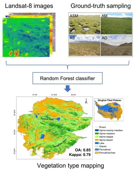
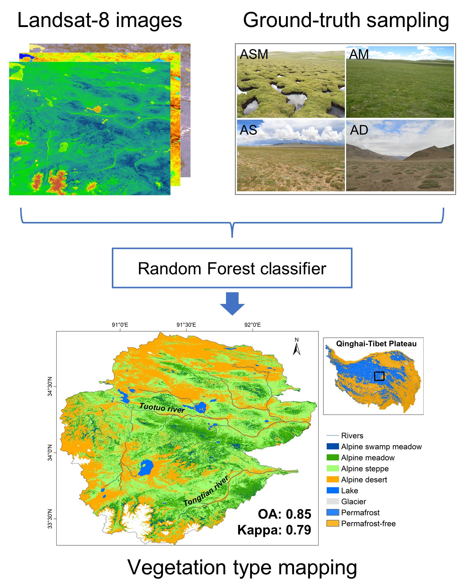
2. Materials and Methods
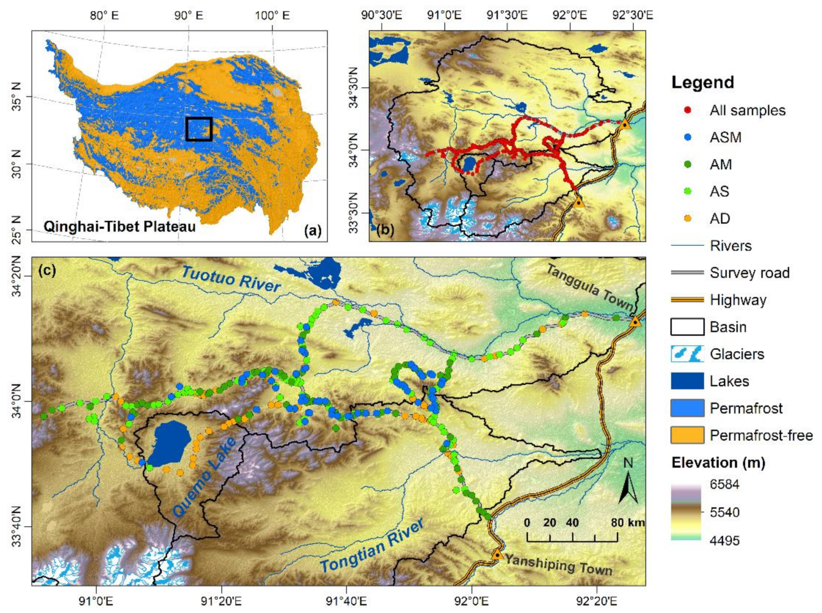
2.1. Study Area

The study area is located on the central QTP and ranges from 90.54 to 92.49° E and from 33.30 to 34.92° N (Figure 1). The study area includes three basins: the Tuotuo River basin, the Tongtian River basin, and the Quemocuo Lake basin, which are the sources of the Yangtze River. They have a total area of 24,980 km2. The basin boundaries were extracted by the ArcSWAT module in Arcmap 10.2 software. The elevation of the study area ranges from 4532 to 6575 m (4980 m on average). Records of the Tuotuohe national meteorological station showed that the mean annual air temperature was −3.4 °C and that the annual precipitation was 303.6 mm (approximately 84% of the precipitation occurred from June to September) during the period 1986–2014 [42]. Permafrost is widely distributed in this study region due to its cold climate conditions [28].

2.2. Data and Processing

2.2.1. The Observational Data

The observational data were collected during roadside surveys across approximately 500 km on the most important areas of natural vegetation during October 2020 (Figure 1). To avoid the influence of the road (very narrow village roads without roadbeds), the location at which each sample was collected was initially designed to be at least 100 m away from the road during the field investigation. The vegetation characteristics at 319 sites were classified into four types: alpine swamp meadow (62), alpine meadow (79), alpine steppe (115), and alpine desert (63). All the locations of the sample sites are registered by a global positioning system (GPS). The elevation and landscape of each site were recorded, and pictures were taken.

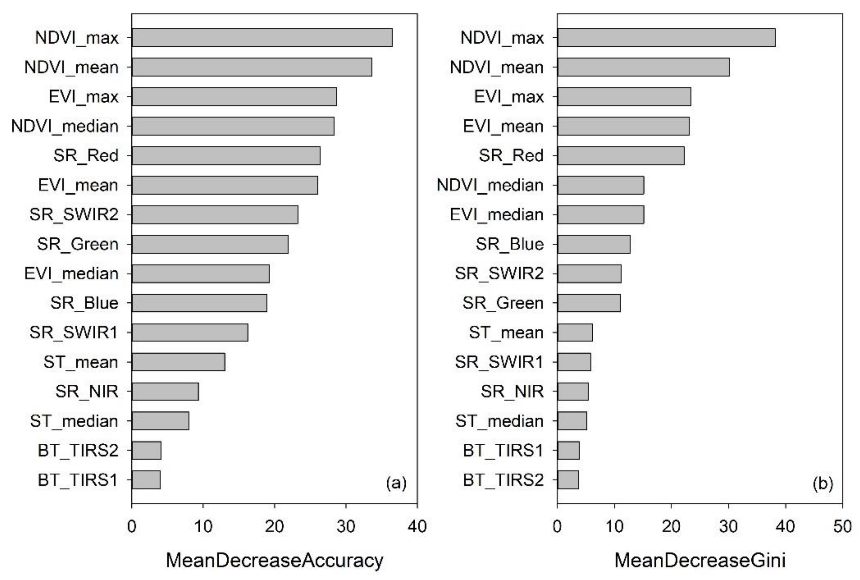
2.2.2. Predictor Variables

In this study, we selected 16 variables derived from Landsat-8 images, including the surface reflectance (SR) of visible and shortwave infrared bands, the brightness temperature (BT) of thermal infrared bands, the enhanced vegetation index (EVI), the normalized difference vegetation index (NDVI), and the surface temperature (ST), to characterize the spatial distribution of the vegetation types. Two products, USGS Landsat 8 Surface Reflectance Tier 1 and Landsat 8 Level 2 Collection 2 Tier 1, were acquired between June and August from 2013 to 2021. For SR and BT, the median values of the cloud-free pixels were extracted as the input variables. Three values (maximum, mean, and median values) for EVI and NDVI and two values (mean and median values) for the ST were extracted during the same period (Table 1). All data processing was accomplished by the Google Earth Engine (GEE) cloud computing platform. The BT and ST bands, while originally collected with a resolution of 100 m, have been resampled using cubic convolution to 30 m in the products.

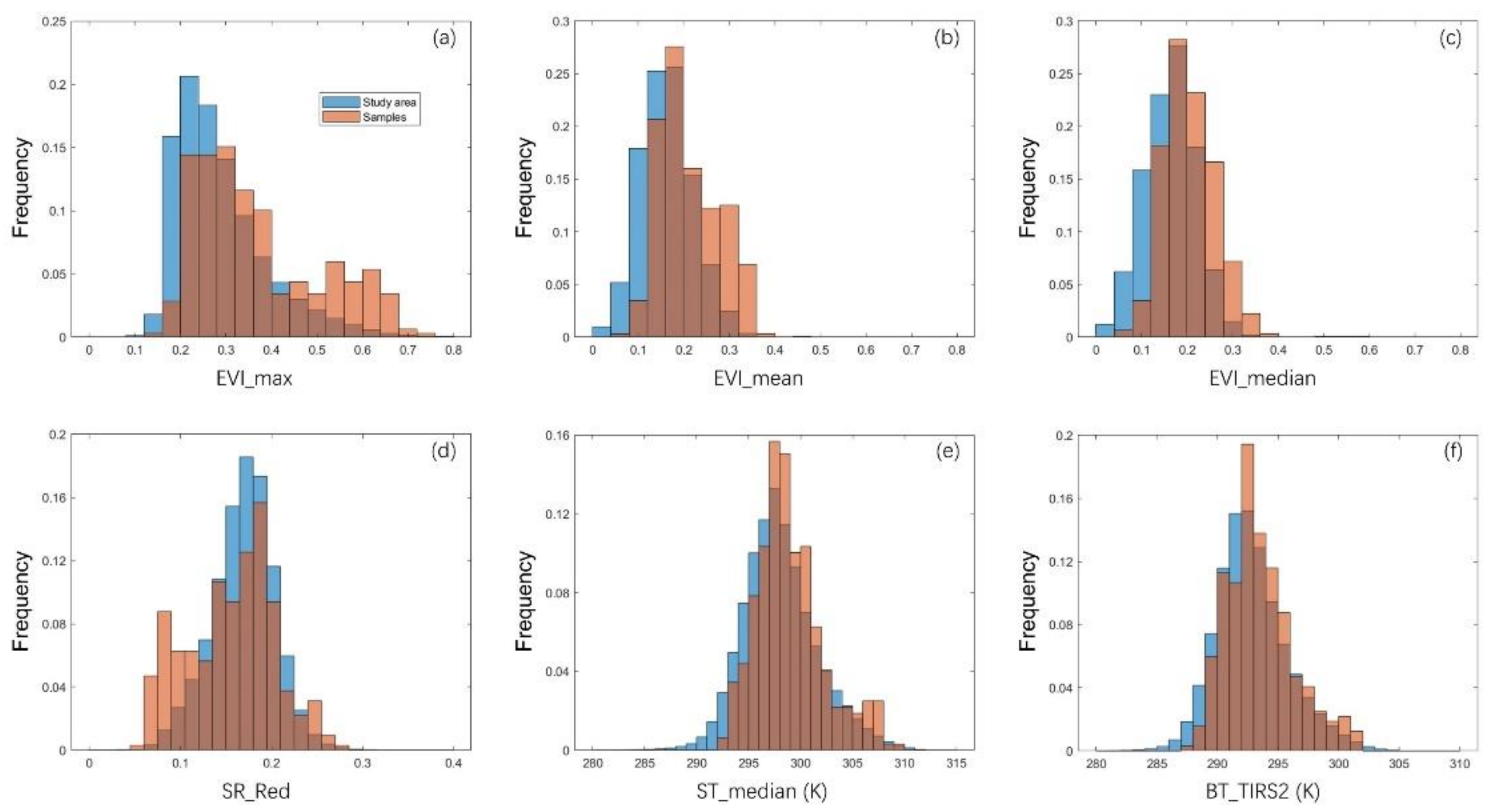
2.2.3. Analysis of Sample Representativeness

The evaluation of sample representativeness was evaluated by frequency histograms. The Euclidean distance and correlation coefficient (r) were used to evaluate the similarity of variable frequency histograms between the samples and the study area (Table 2). The results showed that all Euclidean distances were lower than 10%, ranging from 5.1% to 9.6% with an average value of 7.1%. The correlation coefficient (r) varied between 0.45 and 0.92 with an average value of 0.79. Six of the frequency histograms are shown in Figure 2. For the EVI (Figure 2a–c), the frequency of samples is slightly lower in the low EVI area and slightly higher in the high EVI area. The lower frequency is mainly related to a few samples in the very high elevation areas of the northern, western, and southern edges (Figure 1). A higher frequency means that more ASM samples were collected. SR_Red showed a slightly higher frequency in the very low SR value intervals (Figure 2d), and the frequency patterns of the ST_median and BT_TIRS2 of the samples were very similar to that of the study area (Figure 2e,f). The samples could have credible representativeness for the study area, although a slight deviation remained.

2.3. Methods

The random forest (RF) classifier was selected in this study to predict the vegetation type, which was implemented in R [43] (https://www.r-project.org/ accessed on 12 August 2021). The RF is an ensemble classifier that uses a set of classification and regression trees to make a prediction. In this way, it reduces the overfitting problem in decision trees and reduces their variance, therefore improving accuracy [44,45]. No feature scaling (standardization and normalization) is required, as it uses a rule-based approach instead of a distance calculation [46,47]. Moreover, the RF allows us to assess the importance of each input variable through mean decrease accuracy or mean decrease Gini coefficients [43].
Before formal prediction with the RF classifier, two key parameters need to be set: the number of split variables (mtry) and the number of decision trees to be generated (ntree). In this study, the mtry parameter was determined by the square root of the total input variables [48], which was set as 4. The ntree parameter was set as 1000 because the errors stabilized before this number of classification trees was achieved. After the determination of mtry and ntree, we used the observational data together with the 16 variables to run the RF classifier. The train-test split was used in each run, e.g., 70% of the vegetation samples were randomly selected to train the RF model, while the remaining 30% were used for validation. First, we ran the model a total of 1000 times, and the average overall accuracy and kappa coefficient were used to evaluate the performance of the RF classifier. Then, the top 5% high accuracies of 1000 results, i.e., the 50 results with the highest accuracy, were selected to create the final map. The majority of 50 results was used to determine the vegetation type for each pixel. The averaged confusion matrix and associated classification accuracies, including the overall accuracy, producer accuracy, user accuracy, and kappa coefficient, were employed to evaluate the predicted map. Finally, a percentage of misclassified frequency in the total 1000 times was used to determine the uncertainty of each pixel.
The glaciers and lakes were masked in the process of prediction. The glacier area in the study area was masked by the second glacial catalogue data set of China (v1.0), provided by the National Cryosphere Desert Data Center (http://www.ncdc.ac.cn/ accessed on 20 August 2021). The lake area was masked by the China Lake dataset (1960s–2020) [49], provided by the National Tibetan Plateau Data Center (http://data.tpdc.ac.cn/ accessed on 20 August 2021).

3. Results

3.1. The Accuracy Assessment

The RF model results reached an average overall accuracy of 0.78, ranging from 0.66 to 0.92 after 1000 train-test splits. The average kappa coefficient was 0.69, ranging from 0.52 to 0.89. The detailed confusion matrix and associated classification accuracies of the final predicted vegetation type map are summarized in Table 3. The overall accuracy and kappa coefficient of the map reached 0.848 (0.844–0.852 at a 95% confidence level) and 0.790 (0.785–0.796 at a 95% confidence level), respectively. Most of the producer and user accuracies for all four classified types exceeded 80%. Among the vegetation types, ASM achieved the highest user accuracy with a value of 95.0%, AD had high accuracy (86.7%), while AM and AS achieved the slightly lower, similar accuracies of 83.3% and 82.4%, respectively. In addition, the matrix showed that only one misclassified type was found in ASM and AD, two types were found in AM and AS, and misclassifications occurred only in the adjacent types for each type.
We assessed the importance contribution of all the variables in terms of the mean decrease accuracy and mean decrease Gini coefficients (Figure 3); a larger value means greater contribution of a given variable to vegetation type prediction. Both assessment results of the two coefficients showed that the NDVIs and EVIs were the first two most important variables for vegetation type prediction in the study area, and NDVIs made a slightly larger contribution than that of EVIs; the median SRs of visible and shortwave infrared bands showed a secondary contribution; and the median BTs of thermal infrared bands and the STs showed very little contribution. Additionally, the maximum form of the vegetation indices (i.e., NDVI_max and EVI_max) contributes more than the mean and median forms.

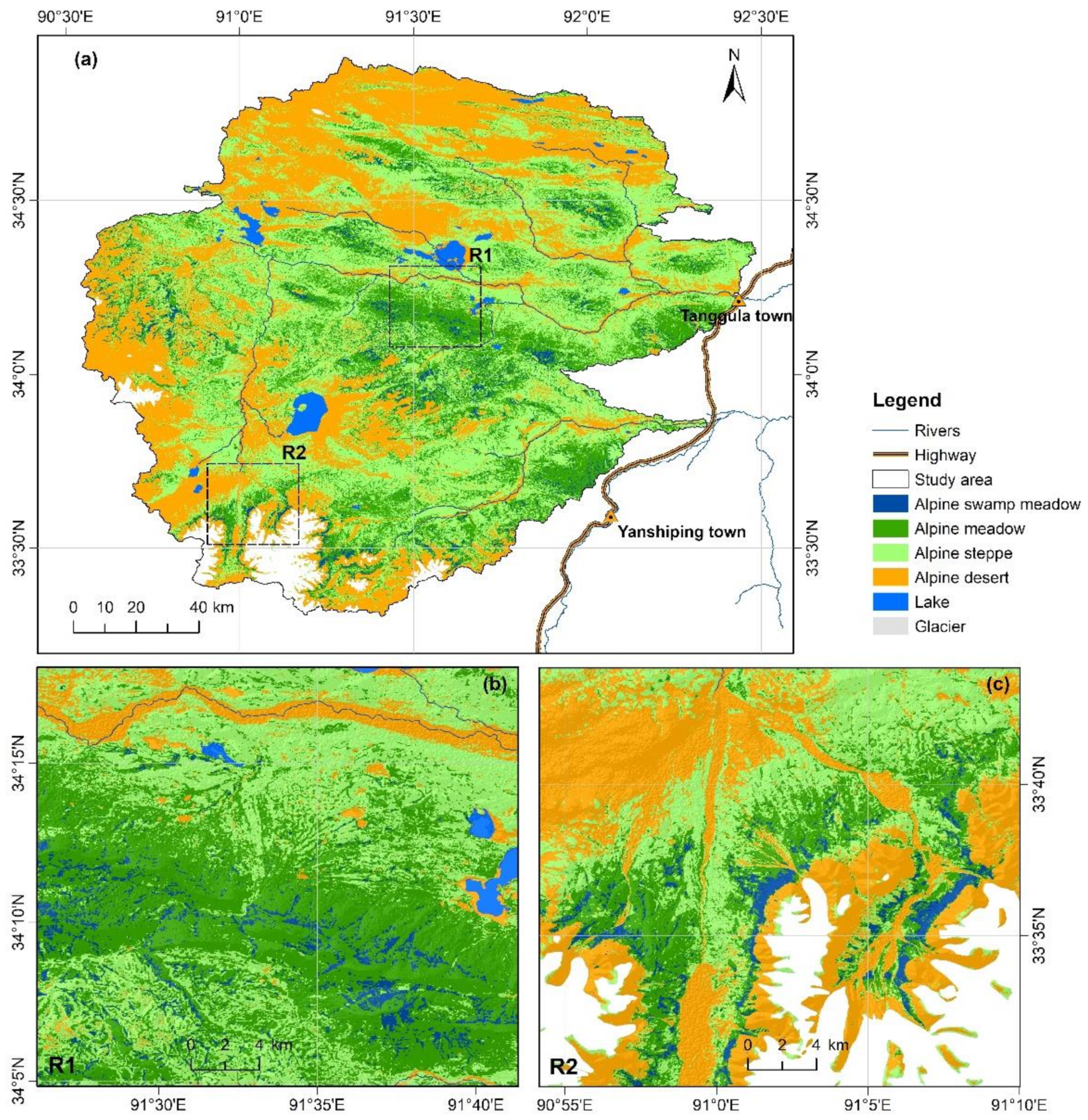
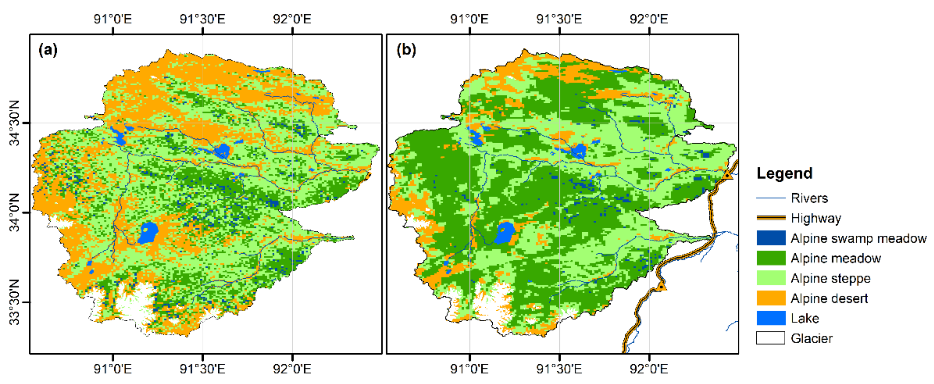
3.2. Vegetation Map in the Study Area

The predicted vegetation type map in this study is shown in Figure 4. The total area of the study region is 24,980 km2, of which 23,927 km2 (95.8%) is vegetated, and the glaciers and lakes cover 708 km2 (2.8%) and 345 km2 (1.4%), respectively. In the vegetated region, the most dominant vegetation types were AS and AD, accounting for 40.2% and 34.0% of the total study area, respectively. Both AS and AD were extensively distributed in the entire study area. The AM and ASM, accounting for 19.0% and 2.5%, respectively, usually showed patchy and discontinuous distribution patterns.
In terms of the spatial pattern of vegetation, the northern and western parts of the study area were dominated by AS and AD, whereas ASM and AM were mainly distributed in the central and southern parts. This pattern also showed a close relationship to the terrain. The ASM and AM were mainly concentrated in the region with high relief, within a set of west-to-east oriented mountain ranges. The AS and AD usually occur in relatively flat regions, e.g., floodplains, terraces, and lake basins. Additionally, a horizontal vegetation pattern was found that was characterized by the sequential occurrence of ASM-AM-AS-AD, i.e., the vegetation types essentially appeared according to this order in this area.
We also selected two regions to show the detailed distribution of vegetation in the predicted map, with region 1 (R1, Figure 4b) located in the central study area and region 2 (R2, Figure 4c) located in the source of the Tuotuo River (i.e., the north side of Geladandong Glacier). In R2, several large areas of ASM appeared on the northern slope of the glacier; however, this phenomenon was rare in other regions of the study area. Most of the distribution patterns of ASM were more similar to those shown in R1, which was characterized by a patchy and sporadic distribution with irregular shapes. These ASMs often occurred at the mountain foot or in a narrow valley alluvium (areas usually ground water outflowed to surface), which usually showed a long strip or fan-like shapes with lengths from dozens of meters to several hundred meters. From Figure 4, both R1 and R2 show that the predicted map at a 30 m resolution can capture the detailed spatial distribution of the ASM well. Moreover, these two regions also exhibited a clearer pattern of the vegetation sequentially occurring from ASM to AD, i.e., according to order of ASM-AM-AS-AD. However, the complete transition distances from ASM to AD were closely related to the terrain. A mountain front alluvial plain with gentle terrain relief in R1 presented a relatively long transition distance, while steep terrain in R2 shortened the distance of a complete transition.

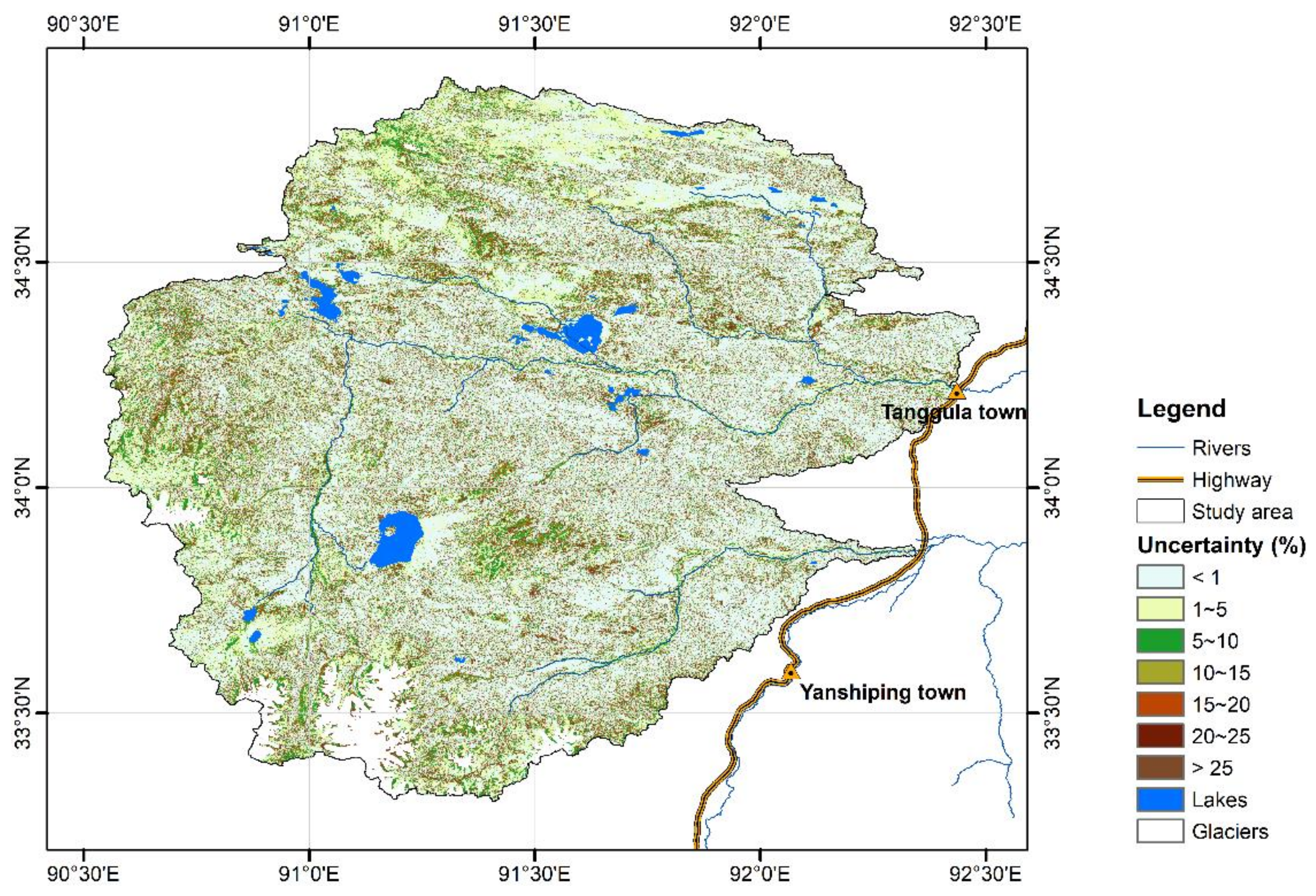
3.3. Uncertainties of the Map

The uncertainty for each pixel was evaluated by a misclassified rate of the predicted type in a total of 1000 train-test splits. Figure 5 shows the spatial pattern of the uncertainties of the map. The results show that the average uncertainty of the map was 6.4% and those of ASM, AM, AS, and AD were 6.8%, 5.9%, 7.2% and 5.8%, respectively. Areas with uncertainties lower than 1% accounted for 48.3% of the vegetated area, and areas with uncertainties lower than 5% and 10% accounted for 67.8% and 76.6%, respectively. Areas with uncertainties greater than 25% and 20% accounted for only 8.9% and 11.3%, respectively.

4. Discussion

In this study, the assessment of contribution importance showed that the vegetation indices (i.e., NDVI and EVI) were the first control factor, the median SRs showed a moderate contribution, and the median BTs and STs contributed little. This suggested that the vegetation growth conditions and the reflectance characteristics of the ground surface contribute more to the vegetation mapping in the study area. This phenomenon is closely related to the climatic and vegetation characteristics of the study area. The climate in the study area belongs to the alpine semi-arid and semi-humid climate transition zone [50], its precipitation decreases from east-south to west-north being mainly controlled by the terrain. Under such precipitation patterns, the spatial distribution of vegetation type also showed a quickly changing pattern in this region. Related to the climate, the study area is also a transition zone of vegetation; with meadow-type vegetation dominating eastward, and steppe- or desert-type vegetation dominating westward [29,30]. These distinctive environmental features make the vegetation types easy to separate from each other based on the vegetation indices and surface reflectance information observed by the remote sensing sensor. In other words, the information from Landsat-8 images (especially for the vegetation indices) can satisfy the vegetation type mapping in this study area, i.e., the transition zone of precipitation and vegetation on the central QTP. However, the result is not always applicable. A study in the source region of the Yellow River of the eastern QTP showed that terrain factors (e.g., slope and aspect) can help to improve vegetation type mapping under the same EVI interval [40]. Therefore, the selection of predictors should be considered according to the climatic and vegetation characteristics of the study area.
The larger contribution of the NDVI to prediction than the EVI could be caused by topographic effects. The soil adjustment factor in the EVI makes it more sensitive to topographic conditions; however, this effect can usually be ignored with the NDVI with only a band ratio format [51]. In addition, the short height and low biomass of vegetation in the study area may not inspire the advantages of the EVI. The vegetation indices, as an integrated variable, performed better than all of the individual, visible, and shortwave infrared bands in this study. The small contribution of the BT and ST could be caused by the diurnal variation in temperature. The pass time of the Landsat-8 satellite coincides with the most rapid warming period in a day, while the temperature fluctuation is usually large due to intense solar radiation and strong wind. In this case, the BT and ST did not remain stable as vegetation indices; therefore, they caused the data to be incomparable between pixels even in a mean or median form.
The classification confusion was related to the spatial pattern of vegetation types in the study area. Generally, four types occurred according to the order of ASM-AM-AS-AD, which can also be observed in Figure 4. In the study area, the ASM is characterized by high coverage (mostly above 80%) and a very wet ground surface (usually holding water bodies in the summer) [39]; these unique features make it easy to differentiate. The other distinct vegetation type with ground surface features is AD, which is characterized by very sparse plants, low vegetation coverage, and dry environments. For that reason, ASM and AD obtained the highest accuracies, as only one adjacent type was misclassified for both, and there was no misclassification between them (Table 3). The main misclassification occurred in AM and AS, influenced by their extensive and mixed distribution patterns. As the most dominant vegetation, AS showed a heterogeneous spatial pattern with concurrent, continuous, and patch distributions. These factors caused an extensive transition area between AS and AM or AD, and the mosaic distribution of different types resulted in more misclassification. The uncertainty map also demonstrated this pattern, with high uncertainties mainly occurring in the transition zone between different types, especially for areas with rapid type changes within short distances.
The distribution of vegetation type in this study was compared with the result provided by Wang et al. (2016) at a spatial resolution of 1 km. The two maps have similar spatial distribution patterns (Figure 6); however, the areas of AM and AS in this study were less than that of Wang et al. (2016), and ASM and AD were greater. The complex terrain relief and the associated precipitation pattern create a heterogeneous vegetation distribution pattern here, and different vegetation types usually appear within a short distance (e.g., dozens of meters). The 1 km resolution map does not often reflect this rapid change, especially for ASM. It was shown that in the western, central, and southern study areas (around the glaciers) (Figure 6), the results of this study identified more patchy areas of ASM than the map of Wang et al. (2016).
The results of this study show that the RF approach can effectively and accurately predict the vegetation classification of permafrost regions on the QTP. Another advantage of the RF approach is that it can detect the main control environmental variables, which can help to further understand the developmental characteristics of vegetation types in different climate zones [52]. Moreover, this study used the last nine years of Landsat data for model input, which can reflect the actual growth of vegetation and eliminate the effects of extreme events on vegetation conditions [40,41]. Based on a spatial resolution of 30 m, the predicted map in this study can provide detailed vegetation information, especially for the distribution of ASM with patches and scattered distribution. To the best of our knowledge, this is the first study to provide a high-resolution vegetation map of this area. The results are promising for further permafrost modeling, and we aim to improve the classification models presented here and to run the methodology across the permafrost region of the QTP.

5. Conclusions

This study mapped the vegetation types using the random forest approach combined with the Landsat-8 images of the central QTP. The performance evaluation showed that the RF approach is useful and effective for vegetation classification in this region, with an average overall accuracy of 0.78 and an average kappa coefficient of 0.69 after 1000 train-test splits. The validation showed that the overall accuracy and kappa coefficient of the predicted map reached 0.848 (0.844–0.852) and 0.790 (0.785–0.796), respectively. Most of the producer and user accuracies for all four classified types exceeded 80%, especially for the ASM, which had the highest user accuracy of 98.4%. The vegetation indices (i.e., NDVI and EVI) are the most important variables in the study area; the surface reflectance of visible and shortwave infrared bands showed a secondary contribution; and the BT and the ST contributed little. The contribution importance of variables is closely related to the climatic and vegetation characteristics of the study area.
The dominant vegetation in the study area is AS and AD, accounting for 40.2% and 34.0% of the total study area, while AM and ASM account for 19.0% and 2.5%, respectively. The ASM and AM usually showed a patchy and discontinuous distribution. The average uncertainty of the map was 6.4%, and those of ASM, AM, AS, and AD were 6.8%, 5.9%, 7.2%, and 5.8%, respectively. The areas with high uncertainties mainly occurred in the transition zone between different types, especially for the boundaries of AM and AS, and in the areas with rapid type changes within short distances. The results of this study showed that the RF approach can effectively and accurately realize the vegetation classification of permafrost regions on the QTP. Based on a spatial resolution of 30 m, the results can provide more detailed vegetation information than the existing maps, which will be helpful for further permafrost modeling in this region.

Author Contributions

D.Z., G.L., E.D., G.H. and Z.L. carried out the fieldwork for sample collection; D.Z. and L.Z. conducted the analysis and prepared the manuscript; L.Z., T.W., X.W. and J.C. provided overall supervision and contributed to the writing and editing. All authors have read and agreed to the published version of the manuscript.

Funding

This research was funded by the Second Tibetan Plateau Scientific Expedition and Research Program (2019QZKK0201), the National Natural Science Foundation of China (41931180, 41690142, 41771076), the West Light Foundation of the Chinese Academy of Sciences, and the State Key Laboratory of Cryospheric Science (SKLCS-ZZ-2022).

Institutional Review Board Statement

Not applicable.

Informed Consent Statement

Not applicable.

Data Availability Statement

Acknowledgments

We are grateful to the anonymous reviewers and editors for appraising our manuscript and for offering instructive comments. We also appreciate the free access of data sets from the National Cryosphere Desert Data Center, the National Tibetan Plateau Data Center, and the Google Earth Engine platform.

Conflicts of Interest

The authors declare no conflict of interest.

References

  1. Küchler, A.W. Vegetation Mapping; Ronald Press Co.: New York, NY, USA, 1967; pp. 853–855. [Google Scholar]
  2. Cannone, N.; Pignatti, S. Ecological responses of plant species and communities to climate warming: Upward shift or range filling processes? Clim. Chang. 2014, 123, 201–214. [Google Scholar] [CrossRef]
  3. Silapaswan, C.S.; Verbyla, D.L.; McGuire, A.D. Land Cover Change on the Seward Peninsula: The Use of Remote Sensing to Evaluate the Potential Influences of Climate Warming on Historical Vegetation Dynamics. Can. J. Remote Sens. 2014, 27, 542–554. [Google Scholar] [CrossRef]
  4. Ahlström, A.; Xia, J.; Arneth, A.; Luo, Y.; Smith, B. Importance of vegetation dynamics for future terrestrial carbon cycling. Environ. Res. Lett. 2015, 10, 54019. [Google Scholar] [CrossRef]
  5. Jiao, Y.; Lei, H.; Yang, D.; Huang, M.; Liu, D.; Yuan, X. Impact of vegetation dynamics on hydrological processes in a semi-arid basin by using a land surface-hydrology coupled model. J. Hydrol. 2017, 551, 116–131. [Google Scholar] [CrossRef]
  6. Hartley, A.J.; MacBean, N.; Georgievski, G.; Bontemps, S. Uncertainty in plant functional type distributions and its impact on land surface models. Remote Sens. Environ. 2017, 203, 71–89. [Google Scholar] [CrossRef]
  7. Harper, A.B.; Wiltshire, A.J.; Cox, P.M.; Friedlingstein, P.; Jones, C.D.; Mercado, L.M.; Sitch, S.; Williams, K.; Duran-Rojas, C. Vegetation distribution and terrestrial carbon cycle in a carbon cycle configuration of JULES4.6 with new plant functional types. Geosci. Model Dev. 2018, 11, 2857–2873. [Google Scholar] [CrossRef] [Green Version]
  8. Recknagel, F. Applications of machine learning to ecological modelling. Ecol. Modell. 2001, 146, 303–310. [Google Scholar] [CrossRef]
  9. Xie, Y.; Sha, Z.; Yu, M. Remote sensing imagery in vegetation mapping: A review. J. Plant Ecol. 2008, 1, 9–23. [Google Scholar] [CrossRef]
  10. Rocchini, D.; Hernández-Stefanoni, J.L.; He, K.S. Advancing species diversity estimate by remotely sensed proxies: A conceptual review. Ecol. Inform. 2015, 25, 22–28. [Google Scholar] [CrossRef]
  11. Gašparović, M.; Dobrinić, D. Comparative Assessment of Machine Learning Methods for Urban Vegetation Mapping Using Multitemporal Sentinel-1 Imagery. Remote Sens. 2020, 12, 1952. [Google Scholar] [CrossRef]
  12. Feng, Q.; Liu, J.; Gong, J. UAV Remote Sensing for Urban Vegetation Mapping Using Random Forest and Texture Analysis. Remote Sens. 2015, 7, 1074–1094. [Google Scholar] [CrossRef] [Green Version]
  13. van Everdingen, R.O. Multi-Language Glossary of Permafrost and Related Ground-Ice Terms; Arctic Institute of North America, University of Calgary: Calgary, AL, Canada, 1998; p. 78. [Google Scholar]
  14. Jorgenson, M.T.; Grosse, G. Remote Sensing of Landscape Change in Permafrost Regions. Permafr. Periglac. 2016, 27, 324–338. [Google Scholar] [CrossRef]
  15. Hu, G.; Zhao, L.; Li, R.; Wu, X.; Wu, T.; Xie, C.; Zhu, X.; Hao, J. Thermal properties of active layer in permafrost regions with different vegetation types on the Qinghai-Tibetan Plateau. Theor. Appl. Climatol. 2019, 139, 983–993. [Google Scholar] [CrossRef]
  16. Nicolsky, D.J.; Romanovsky, V.E.; Panda, S.K.; Marchenko, S.S.; Muskett, R.R. Applicability of the ecosystem type approach to model permafrost dynamics across the Alaska North Slope. J. Geophys. Res. Earth Surf. 2017, 122, 50–75. [Google Scholar] [CrossRef]
  17. Loranty, M.M.; Abbott, B.W.; Blok, D.; Douglas, T.A.; Epstein, H.E.; Forbes, B.C.; Jones, B.M.; Kholodov, A.L.; Kropp, H.; Malhotra, A.; et al. Reviews and syntheses: Changing ecosystem influences on soil thermal regimes in northern high-latitude permafrost regions. Biogeosciences 2018, 15, 5287–5313. [Google Scholar] [CrossRef] [Green Version]
  18. Chasmer, L.; Quinton, W.; Hopkinson, C.; Petrone, R.; Whittington, P. Vegetation Canopy and Radiation Controls on Permafrost Plateau Evolution within the Discontinuous Permafrost Zone, Northwest Territories, Canada. Permafr. Periglac. 2011, 22, 199–213. [Google Scholar] [CrossRef]
  19. Pomeroy, J.W.; Gray, D.M.; Hedstrom, N.R.; Janowicz, J.R. Prediction of seasonal snow accumulation in cold climate forests. Hydrol. Process. 2002, 16, 3543–3558. [Google Scholar] [CrossRef]
  20. Chang, X.; Jin, H.; Zhang, Y.; He, R.; Luo, D.; Wang, Y.; Lü, L.; Zhang, Q. Thermal Impacts of Boreal Forest Vegetation on Active Layer and Permafrost Soils in Northern da Xing’Anling (Hinggan) Mountains, Northeast China. Arct. Antarct. Alp. Res. 2018, 47, 267–279. [Google Scholar] [CrossRef] [Green Version]
  21. Walker, D.A.; Jia, G.J.; Epstein, H.E.; Raynolds, M.K.; Chapin Iii, F.S.; Copass, C.; Hinzman, L.D.; Knudson, J.A.; Maier, H.A.; Michaelson, G.J.; et al. Vegetation-soil-thaw-depth relationships along a low-arctic bioclimate gradient, Alaska: Synthesis of information from the ATLAS studies. Permafr. Periglac. 2003, 14, 103–123. [Google Scholar] [CrossRef]
  22. Kade, A.; Romanovsky, V.E.; Walker, D.A. The n-factor of nonsorted circles along a climate gradient in Arctic Alaska. Permafr. Periglac. 2006, 17, 279–289. [Google Scholar] [CrossRef]
  23. Yue, Y.; Liu, H.; Xue, J.; Li, Y.; Guo, W. Ecological indicators of near-surface permafrost habitat at the southern margin of the boreal forest in China. Ecol. Indic. 2020, 108, 105714. [Google Scholar] [CrossRef]
  24. Westermann, S.; Østby, T.; Gisnås, K.; Schuler, T.; Etzelmüller, B.J.T.C. A ground temperature map of the North Atlantic permafrost region based on remote sensing and reanalysis data. Cryosphere 2015, 9, 1303–1319. [Google Scholar] [CrossRef] [Green Version]
  25. Anderson, J.E.; Douglas, T.A.; Barbato, R.A.; Saari, S.; Edwards, J.D.; Jones, R.M. Linking vegetation cover and seasonal thaw depths in interior Alaska permafrost terrains using remote sensing. Remote Sens. Environ. 2019, 233, 111363. [Google Scholar] [CrossRef]
  26. Fisher, J.P.; Estop-Aragones, C.; Thierry, A.; Charman, D.J.; Wolfe, S.A.; Hartley, I.P.; Murton, J.B.; Williams, M.; Phoenix, G.K. The influence of vegetation and soil characteristics on active-layer thickness of permafrost soils in boreal forest. Glob. Chang. Biol. 2016, 22, 3127–3140. [Google Scholar] [CrossRef]
  27. Raynolds, M.K.; Walker, D.A. Circumpolar relationships between permafrost characteristics, NDVI, and arctic vegetation types. In Ninth International Conference on Permafrost; Institute of Northern Engineering, University of Alaska Fairbanks: Fairbanks, AK, USA, 2008; pp. 1469–1474. [Google Scholar]
  28. Zou, D.; Zhao, L.; Sheng, Y.; Chen, J.; Hu, G.; Wu, T.; Wu, J.; Xie, C.; Wu, X.; Pang, Q.; et al. A new map of permafrost distribution on the Tibetan Plateau. Cryosphere 2017, 11, 2527–2542. [Google Scholar] [CrossRef] [Green Version]
  29. Editorial Board of Vegetation Map of China. 1:1,000,000 Vegetation Atlas of China; Science Press: Beijing, China, 2001. [Google Scholar]
  30. Su, Y.; Guo, Q.; Hu, T.; Guan, H.; Jin, S.; An, S.; Chen, X.; Guo, K.; Hao, Z.; Hu, Y.; et al. An updated Vegetation Map of China (1:1,000,000). Sci. Bull. 2020, 65, 1125–1136. [Google Scholar] [CrossRef]
  31. Ren, J.; Hu, Z.; Zhao, J.; Zhang, D.; Hou, F.; Lin, H.; Mu, X.D. A grassland classification system and its application in China. Rangel. J. 2008, 30, 199–209. [Google Scholar] [CrossRef]
  32. Niu, F.; Gao, Z.; Lin, Z.; Luo, J.; Fan, X. Vegetation influence on the soil hydrological regime in permafrost regions of the Qinghai-Tibet Plateau, China. Geoderma 2019, 354, 113892. [Google Scholar] [CrossRef]
  33. Shang, W.; Wu, X.; Zhao, L.; Yue, G.; Zhao, Y.; Qiao, Y.; Li, Y. Seasonal variations in labile soil organic matter fractions in permafrost soils with different vegetation types in the central Qinghai–Tibet Plateau. Catena 2016, 137, 670–678. [Google Scholar] [CrossRef]
  34. Wu, X.; Zhao, L.; Chen, M.; Fang, H.; Yue, G.; Chen, J.; Pang, Q.; Wang, Z.; Ding, Y. Soil Organic Carbon and Its Relationship to Vegetation Communities and Soil Properties in Permafrost Areas of the Central Western Qinghai-Tibet Plateau, China. Permafr. Periglac. 2012, 23, 162–169. [Google Scholar] [CrossRef]
  35. Yuan, Z.Q.; Jin, H.J.; Wang, Q.F.; Wu, Q.B.; Li, G.Y.; Jin, X.Y.; Ma, Q. Profile distributions of soil organic carbon fractions in a permafrost region of the Qinghai–Tibet Plateau. Permafr. Periglac. 2020, 31, 538–547. [Google Scholar] [CrossRef]
  36. Mu, C.; Abbott, B.W.; Norris, A.J.; Mu, M.; Fan, C.; Chen, X.; Jia, L.; Yang, R.; Zhang, T.; Wang, K.J.E.-S.R. The status and stability of permafrost carbon on the Tibetan Plateau. Earth Sci. Rev. 2020, 211, 103433. [Google Scholar] [CrossRef]
  37. Zhao, L.; Wu, X.; Wang, Z.; Sheng, Y.; Fang, H.; Zhao, Y.; Hu, G.; Li, W.; Pang, Q.; Shi, J.; et al. Soil organic carbon and total nitrogen pools in permafrost zones of the Qinghai-Tibetan Plateau. Sci. Rep. 2018, 8, 3656. [Google Scholar] [CrossRef]
  38. Zhang, X.; Xu, S.; Li, C.; Zhao, L.; Feng, H.; Yue, G.; Ren, Z.; Cheng, G. The soil carbon/nitrogen ratio and moisture affect microbial community structures in alkaline permafrost-affected soils with different vegetation types on the Tibetan plateau. Res. Microbiol. 2014, 165, 128–139. [Google Scholar] [CrossRef]
  39. Wang, Z.; Wang, Q.; Zhao, L.; Wu, X.; Yue, G.; Zou, D.; Nan, Z.; Liu, G.; Pang, Q.; Fang, H.; et al. Mapping the vegetation distribution of the permafrost zone on the Qinghai-Tibet Plateau. J. Mt. Sci. 2016, 13, 1035–1046. [Google Scholar] [CrossRef]
  40. Zhang, X.M.; Yu, S.; Nan, Z.T.; Zhao, L.; Zhou, G.Y.; Yue, G.Y. Vegetation classification of alpine grassland based on decision tree approach in the Wenquan area of the Qinghai-Tibet Plateau. Pratacultural Sci. 2011, 12, 2074–2083. [Google Scholar]
  41. Wang, Z.W.; Shi, J.Z.; Yue, G.Y.; Zhao, L.; Nan, Z.T.; Wu, X.D.; Qiao, Y.P.; Wu, T.H.; Zou, D.F. Assessment of vegetation by object-oriented classification and integration of decision tree classifier in Yushu. Acta Prataculturae Sin. 2013, 22, 62–71. [Google Scholar]
  42. Zhang, F.; Shi, X.; Zeng, C.; Wang, L.; Xiao, X.; Wang, G.; Chen, Y.; Zhang, H.; Lu, X.; Immerzeel, W. Recent stepwise sediment flux increases with climate change in the Tuotuo River in the central Tibetan Plateau. Sci. Bull. 2020, 65, 410–418. [Google Scholar] [CrossRef] [Green Version]
  43. Liaw, A.; Wiener, M. Classification and Regression by Random Forest. R News 2002, 2, 18–22. [Google Scholar]
  44. Pal, M. Random Forest classifier for remote sensing classification. Int. J. Remote Sens. 2005, 26, 217–222. [Google Scholar] [CrossRef]
  45. Breiman, L. Random forests. Mach. Learn. 2001, 45, 5–32. [Google Scholar] [CrossRef] [Green Version]
  46. Rodriguez-Galiano, V.F.; Ghimire, B.; Rogan, J.; Chica-Olmo, M.; Rigol-Sanchez, J.P. An assessment of the effectiveness of a random forest classifier for land-cover classification. ISPRS J. Photogramm. 2012, 67, 93–104. [Google Scholar] [CrossRef]
  47. Belgiu, M.; Drăguţ, L. Random Forest in remote sensing: A review of applications and future directions. ISPRS J. Photogramm. 2016, 114, 24–31. [Google Scholar] [CrossRef]
  48. Gislason, P.O.; Benediktsson, J.A.; Sveinsson, J.R. Random forests for land cover classification. Pattern Recognit. Lett. 2006, 27, 294–300. [Google Scholar] [CrossRef]
  49. Zhang, G.; Yao, T.; Chen, W.; Zheng, G.; Shum, C.K.; Yang, K.; Piao, S.; Sheng, Y.; Yi, S.; Li, J.; et al. Regional differences of lake evolution across China during 1960s–2015 and its natural and anthropogenic causes. Remote Sens. Environ. 2019, 221, 386–404. [Google Scholar] [CrossRef]
  50. Li, H.; Song, K.; Zhang, W.; Li, L.; Jiang, H. Temporal and Spatial Variations of Hydrological Factors in the Source Area of the Yangtze River and Its Responses to Climate Change. Mt. Res. 2017, 35, 129–141. [Google Scholar]
  51. Matsushita, B.; Yang, W.; Chen, J.; Onda, Y.; Qiu, G. Sensitivity of the enhanced vegetation index (EVI) and normalized difference vegetation index (NDVI) to topographic effects: A case study in high-density cypress forest. Sensors 2007, 7, 2636–2651. [Google Scholar] [CrossRef] [PubMed] [Green Version]
  52. Bendini, H.N.; Fonseca, L.M.G.; Schwieder, M.; Rufin, P.; Korting, T.S.; Koumrouyan, A.; Hostert, P. Combining Environmental and Landsat Analysis Ready Data for Vegetation Mapping: A Case Study in the Brazilian Savanna Biome. ISPRS Int. Arch. Photogramm. Remote Sens. Spat. Inf. Sci. 2020, 43, 953–960. [Google Scholar] [CrossRef]
Figure 1. Study area and the sample collection sites (a): the location of study area on the QTP, (b): the outline of study area and location of all samples, (c): color-coded samples for each vegetation type; ASM: alpine swamp meadow, AM: alpine meadow, AS: alpine steppe, AD: alpine desert.
Remotesensing 14 00232 g001
Figure 2. Comparison of the frequencies of six predicted variables between the study area and the samples (a): EVI_max, (b): EVI_mean, (c): EVI_median, (d): SR_Red, (e): ST_median, (f): BT_TIRS2.
Remotesensing 14 00232 g002
Figure 3. Variable importance contribution in terms of mean decrease accuracy (a) and mean decrease Gini (b) coefficients.
Remotesensing 14 00232 g003
Figure 4. The predicted vegetation type map of the study area (a) and two selected regions located in the central (b) R1 and southern boundary (c) R2.
Remotesensing 14 00232 g004
Figure 5. The uncertainties of the predicted vegetation type map in this study.
Remotesensing 14 00232 g005
Figure 6. Comparison between the vegetation type distribution in this study (a), resampling resolution to 1 km and the result of Wang et al. (2016) (b).
Remotesensing 14 00232 g006
Table 1. Description of the selected variables (SR: surface reflectance; BT: brightness temperature; EVI: enhanced vegetation index; NDVI: normalized difference vegetation index; ST: surface temperature).
PredictorDescriptionUnitsData SourceResolution (m)
SR_Bluemedian SR at Blue band%Landsat 8 OLI30
SR_Greenmedian SR at Green band%Landsat 8 OLI30
SR_Redmedian SR at Red band%Landsat 8 OLI30
SR_NIRmedian SR at NIR band%Landsat 8 OLI30
SR_SWIR1median SR at SWIR 1 band%Landsat 8 OLI30
SR_SWIR2median SR at SWIR 2 band%Landsat 8 OLI30
BT_TIRS1median BT at TIRS 1 bandKelvinLandsat 8 TIRS30
BT_TIRS2median BT at TIRS 2 bandKelvinLandsat 8 TIRS30
EVI_maxmaximum EVI value/Landsat 8 OLI30
EVI_meanmean EVI value/Landsat 8 OLI30
EVI_medianmedian EVI value/Landsat 8 OLI30
NDVI_maxmaximum NDVI value/Landsat 8 OLI30
NDVI_meanmean NDVI value/Landsat 8 OLI30
NDVI_medianmedian NDVI value/Landsat 8 OLI30
ST_meanmean ST from TIRS 1KelvinLandsat 8 OLI/TIRS30
ST_medianmedian ST from TIRS 1KelvinLandsat 8 OLI/TIRS30
Table 2. Euclidean distances and correlation coefficients of the variable histograms between the samples and study area.
PredictorsEuclidean Distance (%)Correlation Coefficient (r)
SR_Blue9.60.92
SR_Green9.30.89
SR_Red8.40.87
SR_NIR7.80.92
SR_SWIR15.90.87
SR_SWIR26.00.80
BT_TIRS16.40.90
BT_TIRS26.70.88
EVI_max7.70.66
EVI_mean7.80.56
EVI_median7.30.71
NDVI_max7.10.45
NDVI_mean6.60.58
NDVI_media6.70.71
ST_mean5.80.90
ST_median6.40.89
Table 3. Confusion matrix and associated classification accuracies (ASM: alpine swamp meadow; AM: alpine meadow; AS: alpine steppe; AD: alpine desert; CI: confidence interval).
ASMAMASADTotal SampleUser Accuracy (%)
ASM191002095.0
AM120302483.3
AS022843482.4
AD002131586.7
Total sample20233317
Producer accuracy (%)95.087.084.876.5
Overall accuracy0.848 (0.844~0.852, 95% CI)
Kappa0.790 (0.785~0.796, 95% CI)
Publisher’s Note: MDPI stays neutral with regard to jurisdictional claims in published maps and institutional affiliations.

