
Monitoring Climate Impacts on Annual Forage Production across U.S. Semi-Arid Grasslands

 , , , , , , ,
  and
and
Abstract
:1. Introduction
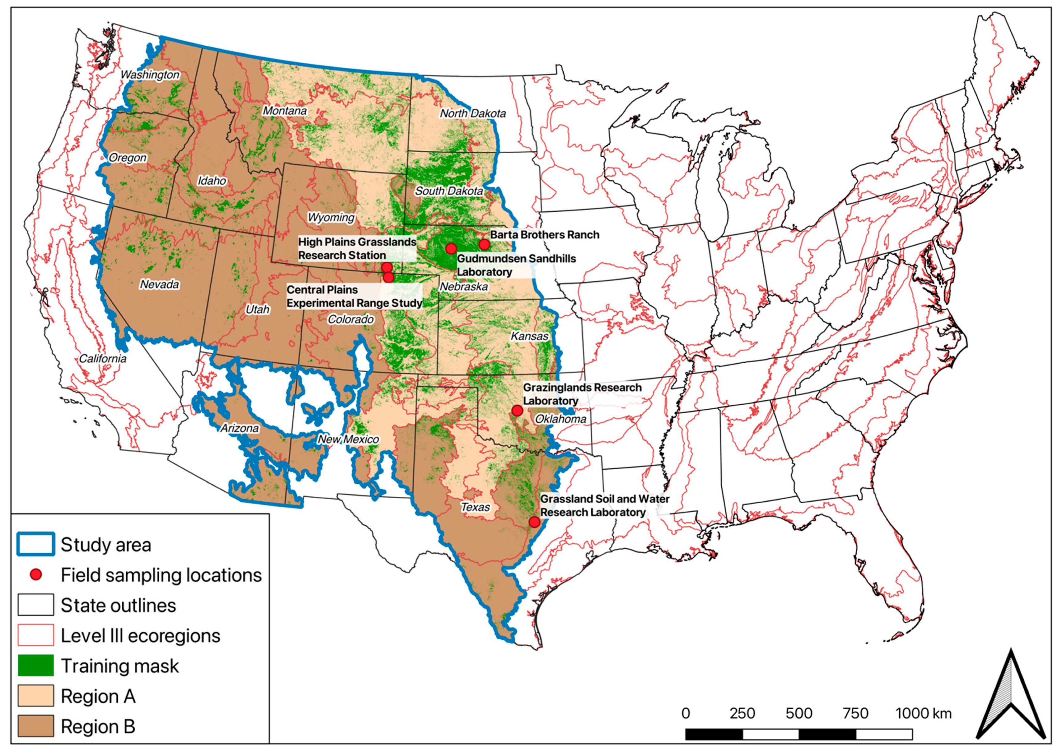
2. Site Description
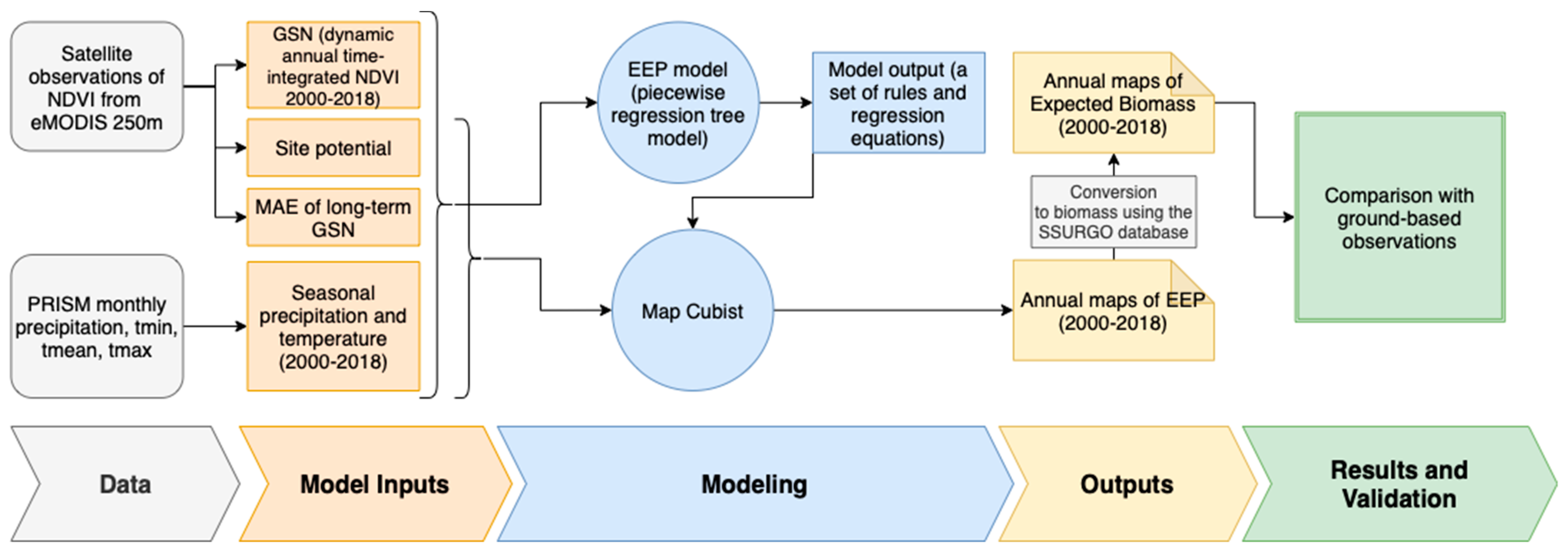
3. Methods
3.1. Model Inputs
3.2. EEP, EB, Annual Biomass Deviation, and Percent Normal Biomass
3.3. Ground Validation
4. Results
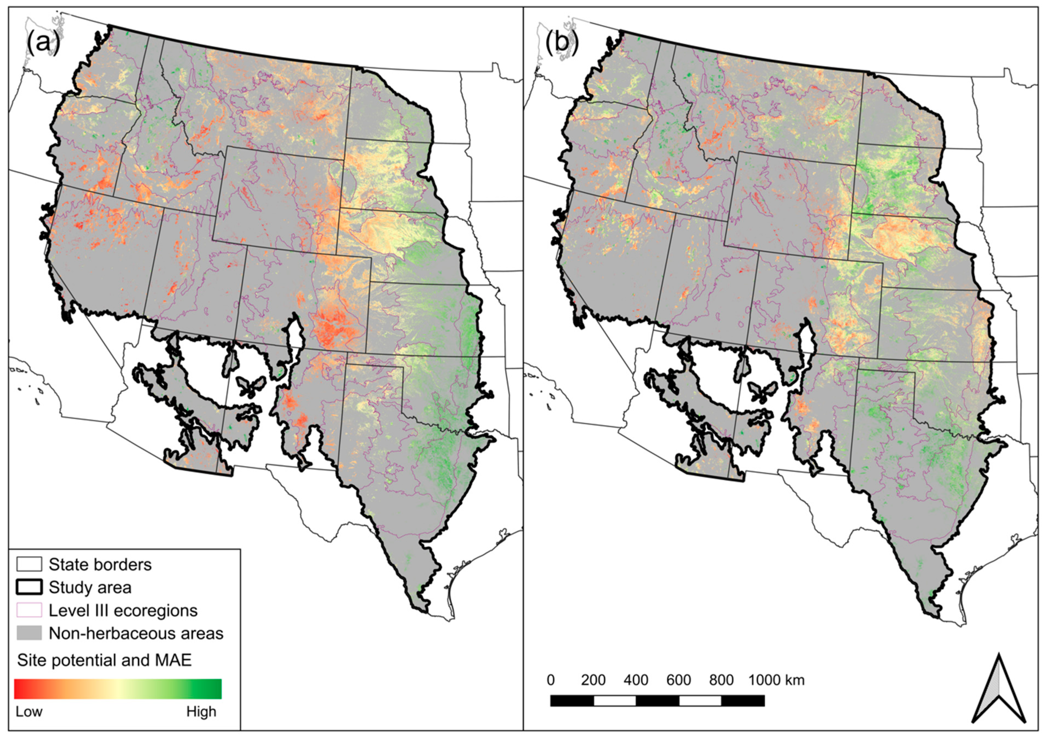
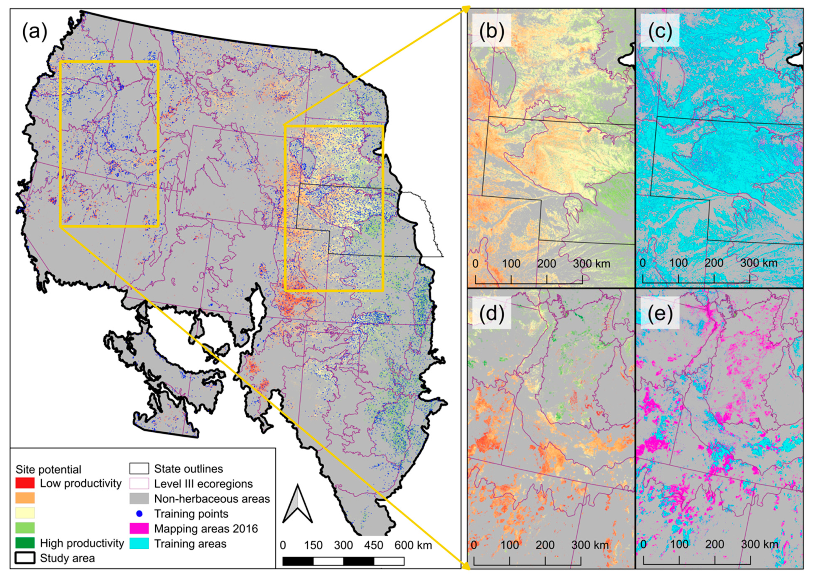
4.1. Site Potential and MAE GSN
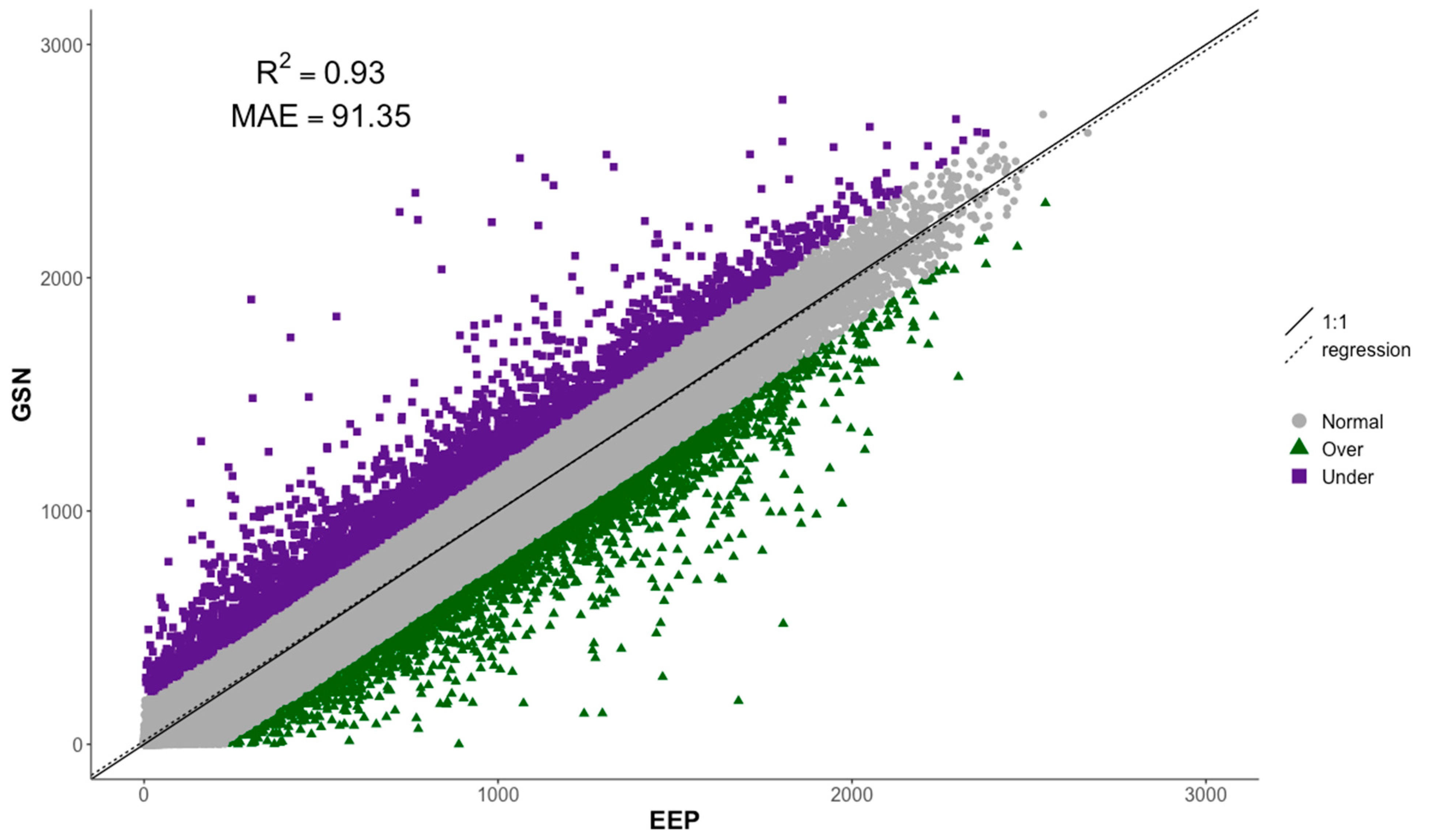
4.2. EEP Model
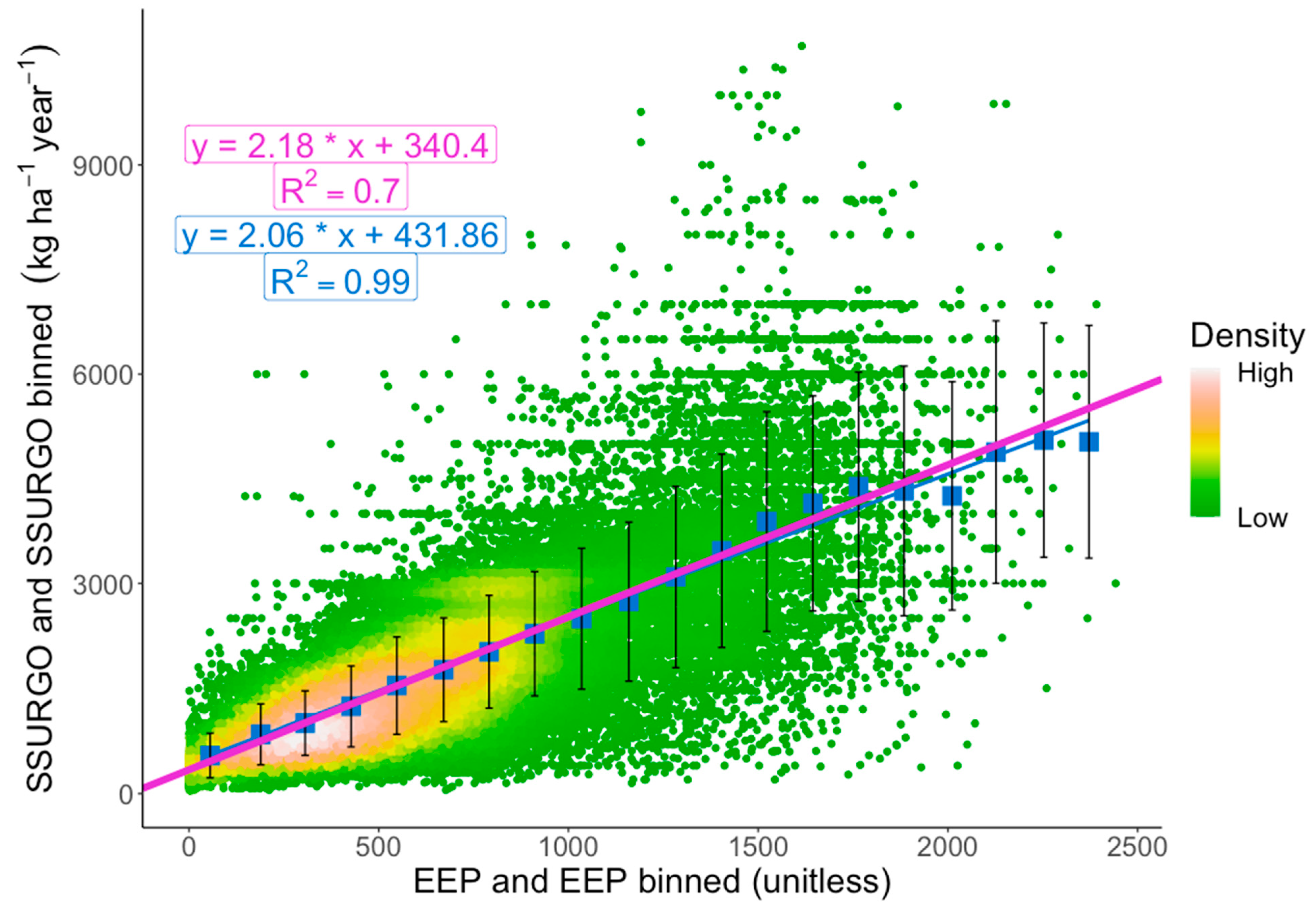
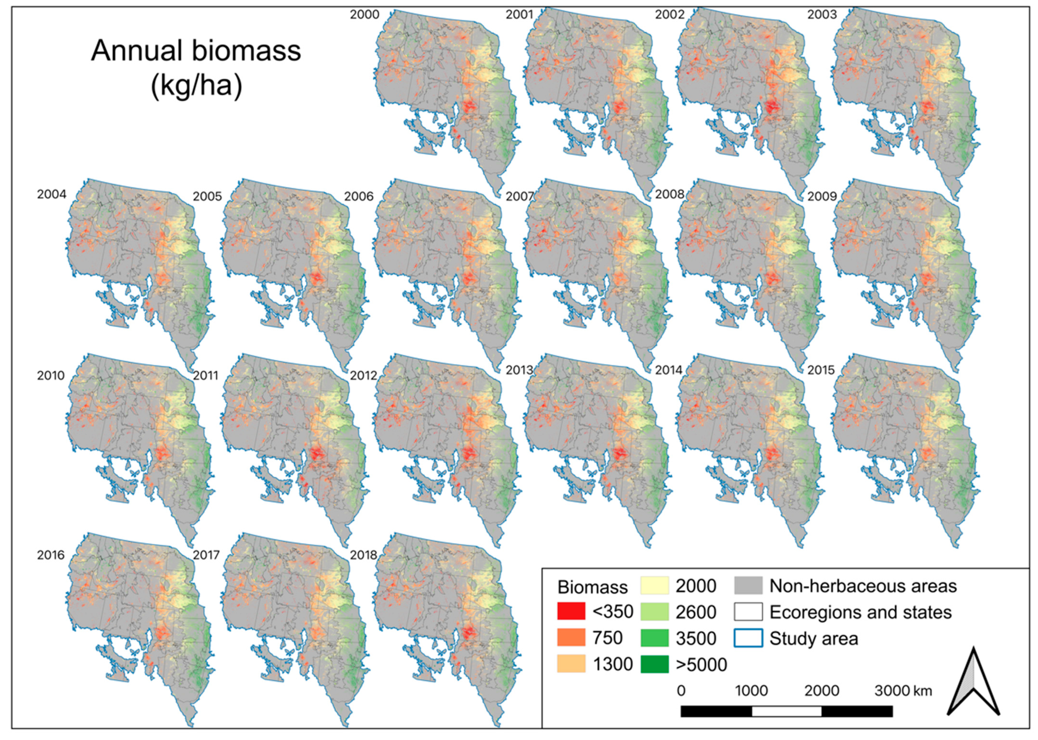
4.3. Conversion to Biomass
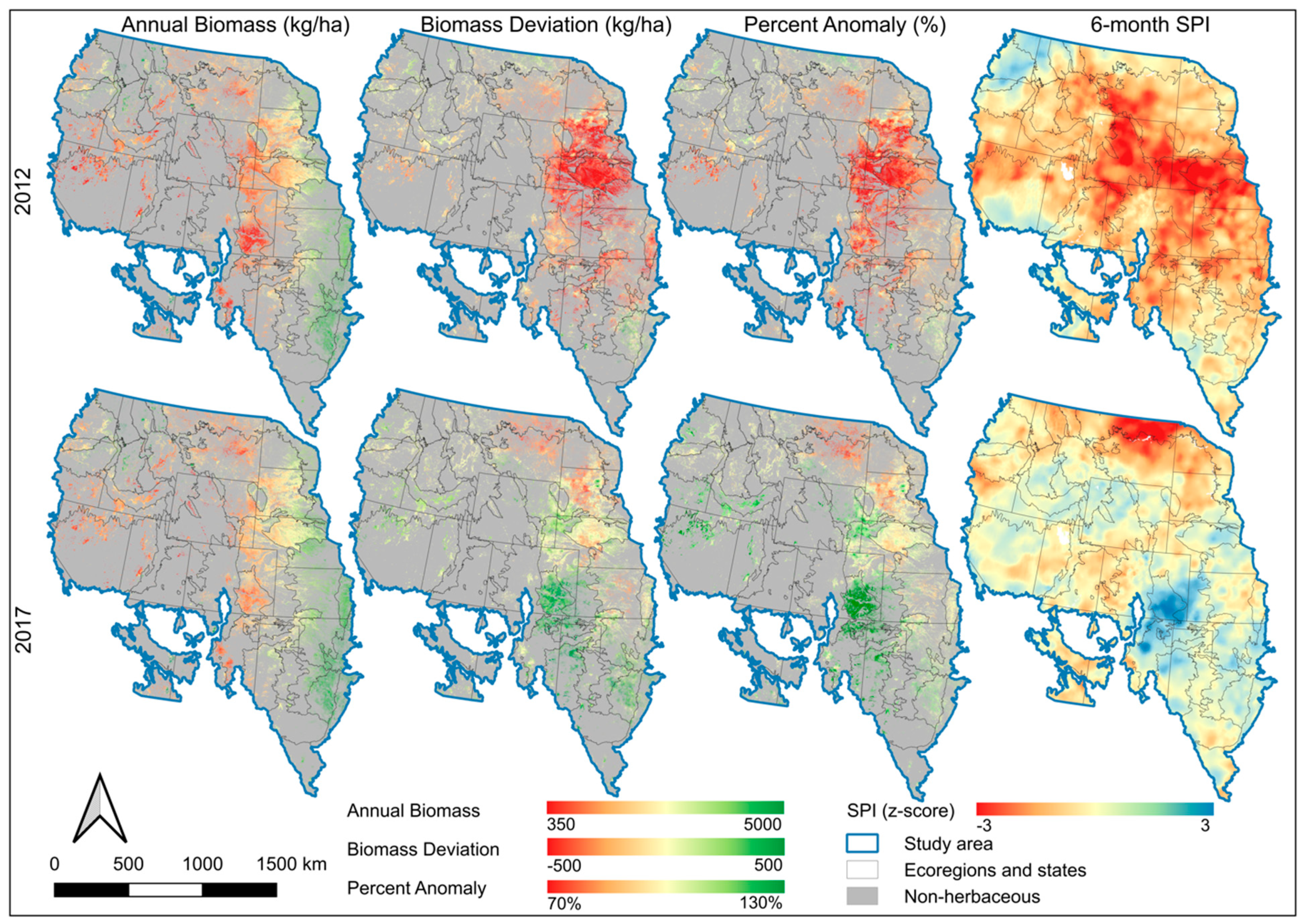
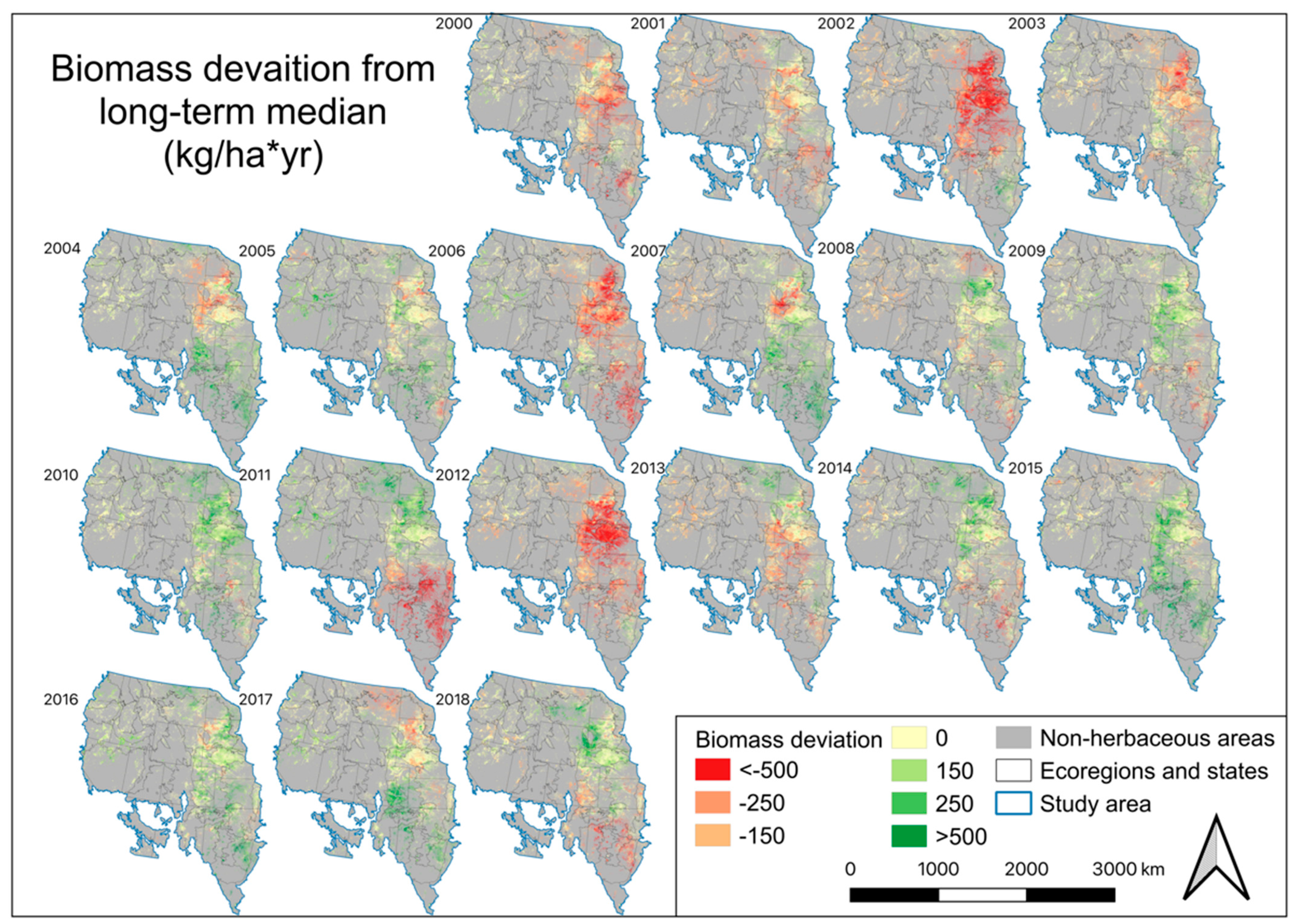
4.4. EB, Annual Biomass Deviation, and Percent Normal Biomass
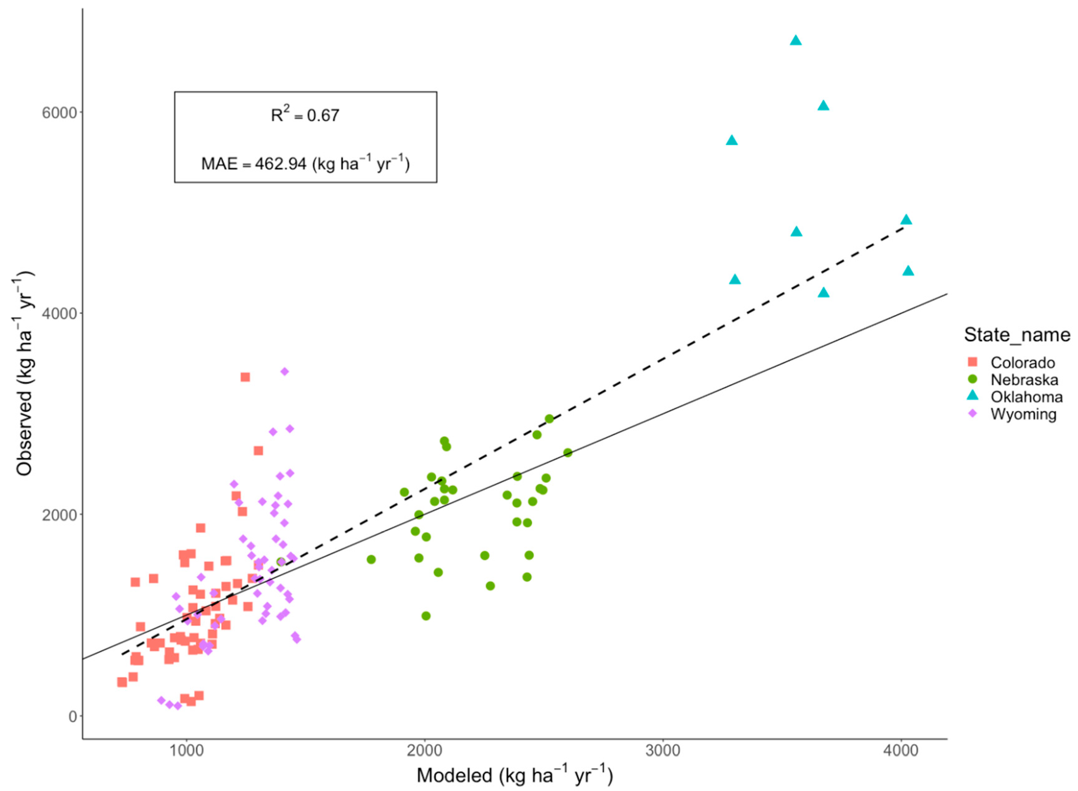
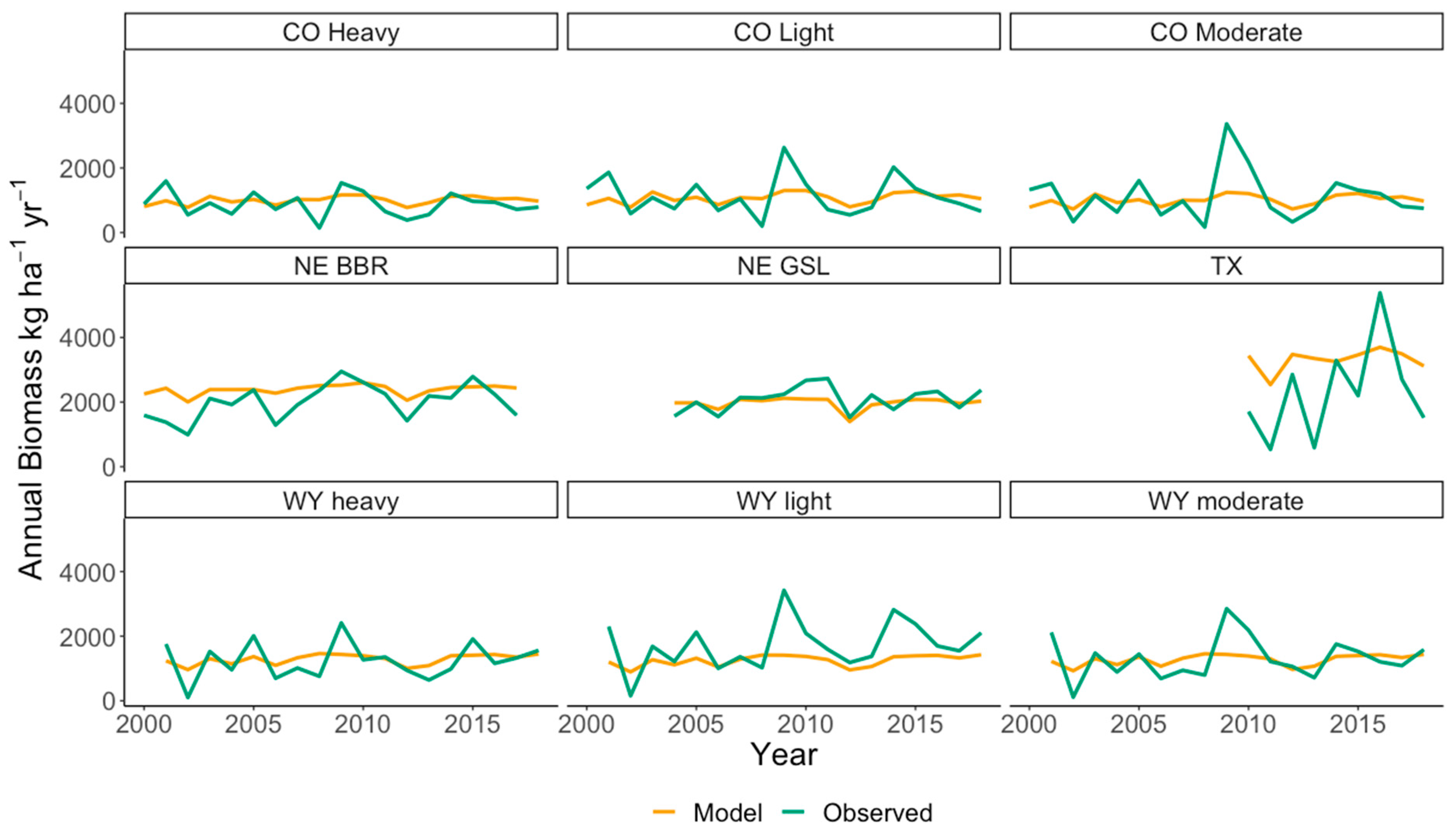
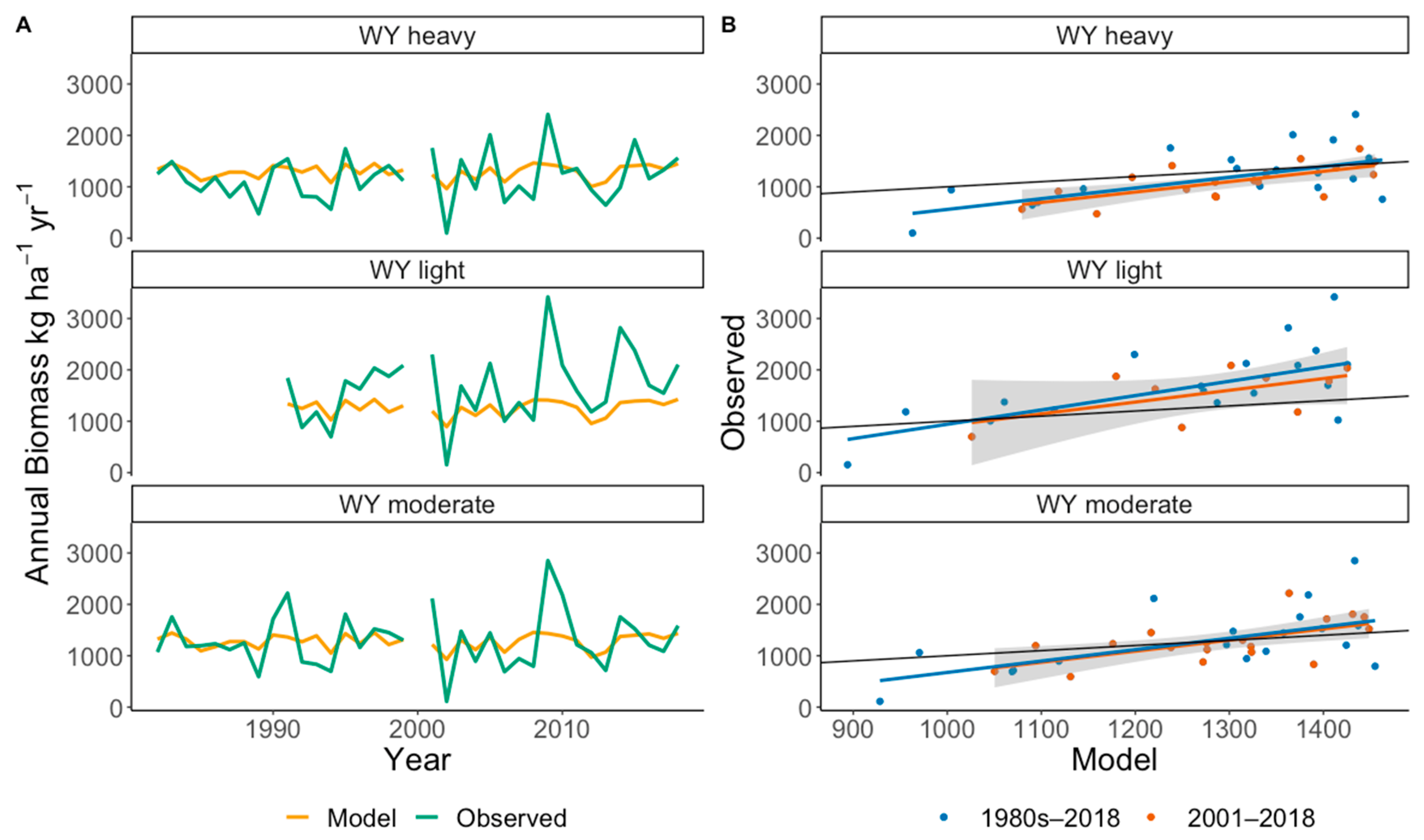
4.5. Validation of the EEP Model
5. Discussion and Conclusions
Author Contributions
Funding
Institutional Review Board Statement
Informed Consent Statement
Data Availability Statement
Acknowledgments
Conflicts of Interest
Appendix A. Delineation of Model Training Areas and Placement of Training Points

| Criteria | Regions | Percent Herbaceous Cover | Percent Water and Wetlands | Percent Cheatgrass Cover | Number of Years Classified as Grassland in NLCD Epochs | Elevation Variation |
|---|---|---|---|---|---|---|
| Training areas | Region A | 100 | 0 | N/A | 7 out of 7 | Standard deviation of elevation in the surrounding 4-km area < 150 m |
| Region B | 80 | 20 | 5 out of 7 | |||
| Mapped areas | Region A | 90 | 10 | N/A | Correspond to the closest NLCD mapping year | Not considered |
| Region B | 75 | 15 |

Appendix B


References
- USDA NRCS Rangelands. Available online: https://www.nrcs.usda.gov/wps/portal/nrcs/detailfull/national/landuse/rangepasture/range/?cid=STELPRDB1043345 (accessed on 1 July 2021).
- Derner, J.; Briske, D.; Reeves, M.; Brown-Brandl, T.; Meehan, M.; Blumenthal, D.; Travis, W.; Augustine, D.; Wilmer, H.; Scasta, D.; et al. Vulnerability of grazing and confined livestock in the Northern Great Plains to projected mid- and late-twenty-first century climate. Clim. Chang. 2018, 146, 19–32. [Google Scholar] [CrossRef]
- Poděbradská, M.; Wylie, B.K.; Hayes, M.J.; Wardlow, B.D.; Bathke, D.J.; Bliss, N.B.; Dahal, D. Monitoring drought impact on annual forage production in semi-arid grasslands: A case study of Nebraska sandhills. Remote Sens. 2019, 11, 2106. [Google Scholar] [CrossRef] [Green Version]
- Reeves, M.C.; Bagne, K.E. Vulnerability of Cattle Production to Climate Change on U.S. Rangelands; US Department of Agriculture, Forest Service: Fort Collins, CO, USA, 2016; 39p.
- Reeves, M.C.; Hanberry, B.B.; Wilmer, H.; Kaplan, N.E.; Lauenroth, W.K. An Assessment of Production Trends on the Great Plains from 1984 to 2017. Rangel. Ecol. Manag. 2021, 78, 165–179. [Google Scholar] [CrossRef]
- Stanke, C.; Kerac, M.; Prudhomme, C.; Medlock, J.; Murray, V. Health effects of drought: A systematic review of the evidence. PLoS Curr. 2013, 5. [Google Scholar] [CrossRef] [Green Version]
- Knutson, C.L.; Haigh, T.R. Ranchers in the United States, scientific information, and drought risk. In Drought, Risk Management, and Policy: Decision-Making under Uncertainty; Botterill, L.C., Cockfield, G., Eds.; CRC Press: Boca Raton, FL, USA, 2013; p. 171. [Google Scholar]
- Rippey, B. Agricultural Weather and Drought Update—8/21/12. Available online: https://www.usda.gov/media/blog/2012/08/21/agricultural-weather-and-drought-update-82112 (accessed on 19 August 2020).
- Rippey, B.U.S. Drought Monitor and USDA Financial Assistance Programs. Available online: http://beef.okstate.edu/files/usdm-and-usda-financial-assistance-programs (accessed on 28 May 2021).
- Leister, A.M.; Paarlberg, P.L.; Lee, J.G. Dynamic effects of drought on US crop and livestock sectors. J. Agric. Appl. Econ. 2015, 47, 261–284. [Google Scholar] [CrossRef] [Green Version]
- Sala, O.E.; Parton, W.J.; Joyce, L.A.; Lauenroth, W.K. Primary production of the central grassland region of the United States. Ecology 1988, 69, 40–45. [Google Scholar] [CrossRef]
- Knapp, A.K.; Smith, M.D. Variation among biomes in temporal dynamics of aboveground primary production. Science 2001, 291, 481–484. [Google Scholar] [CrossRef] [Green Version]
- Derner, J.D.; Hart, R.H. Grazing-induced modifications to peak standing crop in northern mixed-grass prairie. Rangel. Ecol. Manag. 2007, 60, 270–276. [Google Scholar] [CrossRef]
- Derner, J.D.; Augustine, D.J.; Briske, D.D.; Wilmer, H.; Porensky, L.M.; Fernández-Giménez, M.E.; Peck, D.E.; Ritten, J.P. Can Collaborative Adaptive Management Improve Cattle Production in Multipaddock Grazing Systems? Rangel. Ecol. Manag. 2021, 75, 1–8. [Google Scholar] [CrossRef]
- Bement, R.E. A stocking-rate guide for beef production on blue-grama range. Rangel. Ecol. Manag. Range Manag. Arch. 1969, 22, 83–86. [Google Scholar] [CrossRef] [Green Version]
- Raynor, E.J.; Derner, J.D.; Baldwin, T.; Ritten, J.P.; Augustine, D.J. Multidecadal directional shift in shortgrass stocking rates. Rangel. Ecol. Manag. 2021, 74, 72–80. [Google Scholar] [CrossRef]
- Ritten, J.P.; Frasier, W.M.; Bastian, C.T.; Gray, S.T. Optimal rangeland stocking decisions under stochastic and climate-impacted weather. Am. J. Agric. Econ. 2010, 92, 1242–1255. [Google Scholar] [CrossRef]
- Peck, D.; Derner, J.; Parton, W.; Hartman, M.; Fuchs, B. Flexible stocking with Grass-Cast: A new grassland productivity forecast to translate climate outlooks for ranchers. West. Econ. Forum 2019, 17, 24–39. [Google Scholar]
- Derner, J.D.; Augustine, D.J. Adaptive Management for Drought on Rangelands. Rangelands 2016, 38, 211–215. [Google Scholar] [CrossRef] [Green Version]
- Bastian, C.T.; Ritten, J.P.; Derner, J.D. Ranch Profitability Given Increased Precipitation Variability and Flexible Stocking. J. ASFMRA 2018, 122–139. [Google Scholar] [CrossRef]
- Cheng, G.; Harmel, R.D.; Ma, L.; Derner, J.D.; Augustine, D.J.; Bartling, P.N.S.; Fang, Q.X.; Williams, J.R.; Zilverberg, C.J.; Boone, R.B.; et al. Evaluation of APEX modifications to simulate forage production for grazing management decision-support in the Western US Great Plains. Agric. Syst. 2021, 191, 103139. [Google Scholar] [CrossRef]
- Ma, L.; Derner, J.D.; Harmel, R.D.; Tatarko, J.; Moore, A.D.; Rotz, C.A.; Augustine, D.J.; Boone, R.B.; Coughenour, M.B.; Beukes, P.C.; et al. Application of grazing land models in ecosystem management: Current status and next frontiers. Adv. Agron. 2019, 158, 173–215. [Google Scholar] [CrossRef]
- Baumann, M.; Ozdogan, M.; Richardson, A.D.; Radeloff, V.C. Phenology from Landsat when data is scarce: Using MODIS and Dynamic Time-Warping to combine multi-year Landsat imagery to derive annual phenology curves. Int. J. Appl. Earth Obs. Geoinf. 2017, 54, 72–83. [Google Scholar] [CrossRef]
- Zhu, Z.; Woodcock, C.E.; Holden, C.; Yang, Z. Generating synthetic Landsat images based on all available Landsat data: Predicting Landsat surface reflectance at any given time. Remote Sens. Environ. 2015, 162, 67–83. [Google Scholar] [CrossRef]
- Jones, M.O.; Robinson, N.P.; Naugle, D.E.; Maestas, J.D.; Reeves, M.C.; Lankston, R.W.; Allred, B.W. Annual and 16-day rangeland production estimates for the western united states. bioRxiv 2020. [Google Scholar] [CrossRef]
- Hartman, M.D.; Parton, W.J.; Derner, J.D.; Schulte, D.K.; Smith, W.K.; Peck, D.E.; Day, K.A.; Del Grosso, S.J.; Lutz, S.; Fuchs, B.A.; et al. Seasonal grassland productivity forecast for the U.S. Great Plains using Grass-Cast. Ecosphere 2020, 11, e03280. [Google Scholar] [CrossRef]
- Kriegler, F.J.; Malila, W.A.; Nalepka, R.F.; Richardson, W. Preprocessing transformations and their effects on multispectral recognition. Remote Sens. Environ. 1969, VI, 97–132. [Google Scholar]
- AghaKouchak, A.; Farahmand, A.; Melton, F.S.; Teixeira, J.; Anderson, M.C.; Wardlow, B.D.; Hain, C.R. Remote sensing of drought: Progress, challenges and opportunities. Rev. Geophys. 2015, 53, 452–480. [Google Scholar] [CrossRef] [Green Version]
- Ji, L.; Wylie, B.K.; Nossov, D.R.; Peterson, B.; Waldrop, M.P.; McFarland, J.W.; Rover, J.; Hollingsworth, T.N. Estimating aboveground biomass in interior Alaska with Landsat data and field measurements. Int. J. Appl. Earth Obs. Geoinf. 2012, 18, 451–461. [Google Scholar] [CrossRef]
- Wylie, B.K.; Meyer, D.J.; Tieszen, L.L.; Mannel, S. Satellite mapping of surface biophysical parameters at the biome scale over the North American grasslands a case study. Remote Sens. Environ. 2002, 79, 266–278. [Google Scholar] [CrossRef]
- Heim, R.R. A review of twentieth-century drought indices used in the United States. Bull. Am. Meteorol. Soc. 2002, 83, 1149–1165. [Google Scholar] [CrossRef] [Green Version]
- White, A.B.; Kumar, P.; Tcheng, D. A data mining approach for understanding topographic control on climate-induced inter-annual vegetation variability over the United States. Remote Sens. Environ. 2005, 98, 1–20. [Google Scholar] [CrossRef]
- Stephenson, M.B.; Volesky, J.D.; Schacht, W.H.; Lawrence, N.C.; Soper, J.; Milby, J. Influence of Precipitation on Plant Production at Different Topographic Positions in the Nebraska Sandhills. Rangel. Ecol. Manag. 2019, 72, 103–111. [Google Scholar] [CrossRef]
- Lauenroth, W.K.; Sala, O.E. Long-term forage production of North American shortgrass steppe. Ecol. Appl. 1992, 2, 397–403. [Google Scholar] [CrossRef] [PubMed] [Green Version]
- Bradford, J.B.; Lauenroth, W.K.; Burke, I.C.; Paruelo, J.M. The influence of climate, soils, weather, and land use on primary production and biomass seasonality in the US Great Plains. Ecosystems 2006, 9, 934–950. [Google Scholar] [CrossRef]
- Snyman, H.A. Short-term response in productivity following an unplanned fire in a semi-arid rangeland of South Africa. J. Arid Environ. 2004, 56, 465–485. [Google Scholar] [CrossRef]
- Zydenbos, S.M.; Barratt, B.I.P.; Bell, N.L.; Ferguson, C.M.; Gerard, P.J.; Mcneill, M.R.; Phillips, C.B.; Townsend, R.J.; Jackson, T.A. The impact of invertebrate pests on pasture persistence and their interrelationship with biotic and abiotic factors. NZGA Res. Pract. Ser. 2011, 15, 109–117. [Google Scholar] [CrossRef]
- Moran, M.S.; Ponce-Campos, G.E.; Huete, A.; McClaran, M.P.; Zhang, Y.; Hamerlynck, E.P.; Augustine, D.J.; Gunter, S.A.; Kitchen, S.G.; Peters, D.P.C.; et al. Functional response of U.S. grasslands to the early 21st-century drought. Ecology 2014, 95, 2121–2133. [Google Scholar] [CrossRef]
- Petrie, M.D.; Peters, D.P.C.; Yao, J.; Blair, J.M.; Burruss, N.D.; Collins, S.L.; Derner, J.D.; Gherardi, L.A.; Hendrickson, J.R.; Sala, O.E.; et al. Regional grassland productivity responses to precipitation during multiyear above-and below-average rainfall periods. Glob. Chang. Biol. 2018, 24, 1935–1951. [Google Scholar] [CrossRef]
- Wylie, B.; Zhang, L.; Bliss, N.; Ji, L.; Tieszen, L.L.; Jolly, W.M. Integrating modelling and remote sensing to identify ecosystem performance anomalies in the boreal forest, Yukon River Basin, Alaska. Int. J. Digit. Earth 2008, 1, 196–220. [Google Scholar] [CrossRef]
- Omernik, J.M. Ecoregions: A framework for managing ecosystems. Georg. Wright Forum 1995, 12, 35–50. [Google Scholar]
- Sala, O.E.; Paruelo, J.M. Ecosystem Services in Grasslands. In Nature’s Services: Societal Dependence on Natural Ecosystems; Daily, G.C., Ed.; Island Press: Washington, DC, USA, 1997; pp. 237–251. [Google Scholar]
- Hayhoe, K.; Wuebbles, D.J.; Easterling, D.R.; Fahey, D.W.; Doherty, S.; Kossin, J.; Sweet, W.; Vose, R.; Wehner, M. Our Changing Climate. In Impacts, Risks, and Adaptation in the United States: Fourth National Climate Assessment; Reidmiller, D.R., Avery, C.W., Easterling, D.R., Kunkel, K.E., Lewis, K.L.M., Maycock, T.K., Stewart, B.C., Eds.; U.S. Global Change Research Program: Washington, DC, USA, 2018; Volume II. [Google Scholar]
- Quinlan, J.R. Learning with continuous classes. In Proceedings of the 5th Australian joint conference on artificial intelligence, Hobart, Australia, 16–18 November 1992; pp. 343–348. [Google Scholar]
- Boyte, S.P.; Wylie, B.K.; Major, D.J. Mapping and monitoring cheatgrass dieoff in rangelands of the Northern Great Basin, USA. Rangel. Ecol. Manag. Manag. 2015, 68, 18–28. [Google Scholar] [CrossRef]
- Boyte, S.P.; Wylie, B.K.; Gu, Y.; Major, D.J. Estimating Abiotic Thresholds for Sagebrush Condition Class in the Western United States. Rangel. Ecol. Manag. 2020, 73, 297–308. [Google Scholar] [CrossRef]
- Gu, Y.; Wylie, B.K. Detecting ecosystem performance anomalies for land management in the Upper Colorado River Basin using satellite observations, climate data, and ecosystem models. Remote Sens. 2010, 2, 1880–1891. [Google Scholar] [CrossRef] [Green Version]
- Rigge, M.; Wylie, B.; Gu, Y.; Belnap, J.; Phuyal, K.; Tieszen, L. Monitoring the status of forests and rangelands in the Western United States using ecosystem performance anomalies. Int. J. Remote Sens. 2013, 34, 4049–4068. [Google Scholar] [CrossRef]
- RuleQuest Research Cubist; Version 2.07; RuleQuest Research Pty Ltd.: St Ives, NSW, Australia, 2008.
- Wylie, B.K.; Boyte, S.P.; Major, D.J. Ecosystem performance monitoring of rangelands by integrating modeling and remote sensing. Rangel. Ecol. Manag. 2012, 65, 241–252. [Google Scholar] [CrossRef]
- El-Vilaly, M.A.S.; Didan, K.; Marsh, S.E.; van Leeuwen, W.J.D.; Crimmins, M.A.; Munoz, A.B. Vegetation productivity responses to drought on tribal lands in the four corners region of the Southwest USA. Front. Earth Sci. 2018, 12, 37–51. [Google Scholar] [CrossRef]
- Tieszen, L.L.; Reed, B.C.; Bliss, N.B.; Wylie, B.K.; DeJong, D.D. NDVI, C3 and C4 production, and distributions in Great Plains grassland land cover classes. Ecol. Appl. 1997, 7, 58–78. [Google Scholar] [CrossRef]
- Yang, L.; Wylie, B.K.; Tieszen, L.L.; Reed, B.C. An analysis of relationships among climate forcing and time-integrated NDVI of grasslands over the U.S. northern and central Great Plains. Remote Sens. Environ. 1998, 65, 25–37. [Google Scholar] [CrossRef]
- Jenkerson, C.; Maiersperger, T.; Schmidt, G. eMODIS: A User-Friendly Data Source; USGS: Denver, CO, USA, 2010.
- Swets, D.L.; Reed, B.C.; Rowland, J.D.; Marko, S.E. A weighted least-squares approach to temporal smoothing of NDVI. In Proceedings of the ASPRS Annual Conference, From Image to Information; American Society for Photogrammetry and Remote Sensing, Bethesda: Portland, OR, USA, 1999. [Google Scholar]
- Montandon, L.M.; Small, E.E. The impact of soil reflectance on the quantification of the green vegetation fraction from NDVI. Remote Sens. Environ. 2008, 112, 1835–1845. [Google Scholar] [CrossRef]
- PRISM Climate Group PRISM Climate Group. Available online: http://prism.oregonstate.edu/ (accessed on 10 October 2020).
- Pastick, N.J.; Wylie, B.K.; Rigge, M.B.; Dahal, D.; Boyte, S.P.; Jones, M.O.; Allred, B.W.; Parajuli, S.; Wu, Z. Rapid Monitoring of the Abundance and Spread of Exotic Annual Grasses in the Western United States Using Remote Sensing and Machine Learning. AGU Adv. 2021, 2, e2020AV000298. [Google Scholar] [CrossRef]
- Gu, Y.; Wylie, B.K.; Boyte, S.P.; Picotte, J.; Howard, D.M.; Smith, K.; Nelson, K.J. An optimal sample data usage strategy to minimize overfitting and underfitting effects in regression tree models based on remotely-sensed data. Remote Sens. 2016, 8, 943. [Google Scholar] [CrossRef] [Green Version]
- McKee, T.B.; Doesken, N.J.; Kleist, J. The relationship of drought frequency and duration to time scales. In Proceedings of the Eighth Conference on Applied Climatology, Anaheim, CA, USA, 17–22 January 1993. [Google Scholar]
- Irisarri, J.G.N.; Derner, J.D.; Porensky, L.M.; Augustine, D.J.; Reeves, J.L.; Mueller, K.E. Grazing intensity differentially regulates ANPP response to precipitation in North American semiarid grasslands. Ecol. Appl. 2016, 26, 1370–1380. [Google Scholar] [CrossRef] [Green Version]
- Wagle, P.; Gowda, P.H.; Northup, B.K.; Starks, P.J.; Neel, J.P.S. Response of tallgrass prairie to management in the U.S. Southern great plains: Site descriptions, management practices, and eddy covariance instrumentation for a Long-Term Experiment. Remote Sens. 2019, 11, 1988. [Google Scholar] [CrossRef] [Green Version]
- RuleQuest Research An Overview of Cubist. Available online: https://www.rulequest.com/cubist-win.html#CTTEE (accessed on 28 May 2021).
- Poděbradská, M.; Wylie, B.K.; Dahal, D. Time Series of Expected Livestock Forage Biomass in the Semi-Arid Grasslands of the Western U.S. (2000–2018); U.S. Geological Survey Data Release: Reston, VA, USA, 2021. [CrossRef]
- Gu, Y.; Wylie, B.K.; Bliss, N.B. Mapping grassland productivity with 250-m eMODIS NDVI and SSURGO database over the Greater Platte River Basin, USA. Ecol. Indic. 2013, 24, 31–36. [Google Scholar] [CrossRef]
- Asrar, G.Q.; Fuchs, M.; Kanemasu, E.T.; Hatfield, J.L. Estimating absorbed photosynthetic radiation and leaf area index from spectral reflectance in wheat 1. Agron. J. 1984, 76, 300–306. [Google Scholar] [CrossRef]
- Chen, P.-Y.; Fedosejevs, G.; Tiscareno-Lopez, M.; Arnold, J.G. Assessment of MODIS-EVI, MODIS-NDVI and VEGETATION-NDVI composite data using agricultural measurements: An example at corn fields in western Mexico. Environ. Monit. Assess. 2006, 119, 69–82. [Google Scholar] [CrossRef] [PubMed]
- Gaffney, R.; Porensky, L.M.; Gao, F.; Irisarri, J.G.; Durante, M.; Derner, J.D.; Augustine, D.J. Using APAR to predict aboveground plant productivity in semi-aid rangelands: Spatial and temporal relationships differ. Remote Sens. 2018, 10, 1474. [Google Scholar] [CrossRef] [Green Version]
- Wylie, B.K.; DeJong, D.D.; Tieszen, L.L.; Biondini, M.E. Grassland canopy parameters and their relationships to remotely sensed vegetation indices in the nebraska sand hills. Geocarto Int. 1996, 11, 39–52. [Google Scholar] [CrossRef]
- Chaney, N.W.; Wood, E.F.; McBratney, A.B.; Hempel, J.W.; Nauman, T.W.; Brungard, C.W.; Odgers, N.P. POLARIS: A 30-m probabilistic soil series map of the contiguous United States. Geoderma 2016, 274, 54–67. [Google Scholar] [CrossRef] [Green Version]
- Pastick, N.J.; Dahal, D.; Wylie, B.K.; Parajuli, S.; Boyte, S.P.; Wu, Z. Characterizing land surface phenology and exotic annual grasses in dryland ecosystems using landsat and sentinel-2 data in harmony. Remote Sens. 2020, 12, 725. [Google Scholar] [CrossRef] [Green Version]
- Pastick, N.J.; Wylie, B.K.; Wu, Z. Spatiotemporal analysis of Landsat-8 and Sentinel-2 data to support monitoring of dryland ecosystems. Remote Sens. 2018, 10, 791. [Google Scholar] [CrossRef] [Green Version]
- Boyte, S.P.; Wylie, B.K.; Major, D.J. Cheatgrass percent cover change: Comparing recent estimates to climate change—Driven predictions in the Northern Great Basin. Rangel. Ecol. Manag. 2016, 69, 265–279. [Google Scholar] [CrossRef]
- Barry, R.G. Mountain Weather and Climate; Psychology Press: Hove, UK, 1992. [Google Scholar]
- Omernik, J.M. Ecoregions of the Conterminous United States. Ann. Assoc. Am. Geogr. 1987, 77, 118–125. [Google Scholar] [CrossRef]


| Tool Name | Focus | Method | Spatial Resolution | Extent | Limitations | Website | Reference |
|---|---|---|---|---|---|---|---|
| Rangeland Production Monitoring Service (RPMS) | Post-growing season assessment of forage production | Season-maximum Normalized Difference Vegetation Index (NDVI) is linked to ground-observed data | 30 m/250 m | Contiguous U.S. rangelands | The maximum NDVI approach can lead to erroneous estimations in areas with two distinct vegetation peaks, which is characteristic for rangeland plant communities composed of both cool- and warm-season plants and for areas with monsoon influence. | https://www.fuelcast.net (last accessed 18 November 2021) | [5] |
| Rangeland Analysis Platform (RAP) | Post-growing season assessment of forage production | Process-based model that uses Landsat observations. | 30 m | Western U.S. | Long return intervals of Landsat (16-days) with frequent cloud contamination can introduce errors in these observations [23,24] | https://rangelands.app (last accessed 18 November 2021) | [25] |
| Grass-Cast | Within-growing season prediction production anomaly | Process-based model connected with empirical biomass observations. | 10 km | Great Plains and Southwest | Coarse spatial resolution when compared to an average size of a ranch. | https://grasscast.unl.edu (last accessed 18 November 2021) | [18,26] |
| FuelCast | Within-growing season prediction of forage production | Statistical model using empirical relations, climate and remotely sensed NDVI data. | 30 m/250 m | Western U.S. | No peer-reviewed validation of the predictions. | https://www.fuelcast.net (last accessed 18 November 2021) | N/A |
| South Dakota Drought Tool (SDDT) | Within-growing season prediction of percent normal forage production | Empirically established relation between precipitation and production. | N/A | South Dakota | No peer-reviewed publication, no formal validation of the predictions, limited spatial extent. | https://www.nrcs.usda.gov/wps/portal/nrcs/main/sd/technical/landuse/pasture/ (last accessed 18 November 2021) | N/A |
| Location. | Research Station | Site Name | Method of Data Collection | Validation Years | Source | More Info |
|---|---|---|---|---|---|---|
| Whitman, Nebraska | Gudmundsen Sandhills Laboratory, | NE GSL | Each pasture contained multiple 0.25-m2 exclosed cages in pastures grazed the previous year. Biomass clipping was performed in mid-August, which was considered peak production for warm-season grasses for that year. Clipping samples were dried and weighed. | 2004–2018 | UNL | [33] |
| Bassett, Nebraska | Barta Brothers Ranch | NE BBR | 2000–2017 | |||
| Nunn, Colorado | Central Plains Experimental Range Study | CO Light | Each pasture (~130 ha) contained 12 temporarily exclosed cages that were annually moved. Biomass clipping was performed in early August, which is considered peak production in this system. Different grazing pressures were applied for the three sites—light, moderate, and heavy. Clipping samples were dried and weighed. | 2000–2018 | USDA ARS | [61] |
| CO Moderate | ||||||
| CO Heavy | ||||||
| Cheyenne, Wyoming | High Plains Grasslands Research Station | WY Light | Each pasture contained 3 temporarily exclosed cages that were randomly moved each year along a 50-m permanent transect. The sites were of different size and grazing pressure—WY Light ~80 ha, WY Moderate ~12 ha, and WY Heavy ~8 ha—and grass clipping was performed in mid-July, which is considered peak production in this system. Clipping samples were dried and weighed. | 1982–1999, 2001–2018 | USDA ARS | [13,61] |
| WY Moderate | ||||||
| WY Heavy | ||||||
| El Reno, Oklahoma | Grazinglands Research Laboratory | OK P11 | Clipping samples were collected destructively from 0.25-m2 quadrats and collected in five random locations along a 100-m transect in the north-south directions. The clipping areas were not located in exclosed cages and therefore the measurements represent biomass under low grazing pressure. Clipping samples were dried and weighed. | 2014–2016, 2018 | USDA ARS | [62] |
| OK P13 | ||||||
| Temple, Texas | Grassland Soil and Water Research Laboratory | TX | Large stands (0.25–0.37 ha) were planted with switchgrass or a mixture of native grassland species. At the end of the growing season, the stands were harvested with typical haying equipment. Hay bales were weighed and converted to kg ha−1 to represent the entire stand. For the purpose of this study, the stands were averaged each year. The grass samples were not dried. | 2010–2018 | USDA ARS | N/A |
| Independent Variable | Overall Importance (%) |
|---|---|
| Site Potential | 80.5 |
| Summer Precipitation | 77.0 |
| MAE | 69.0 |
| Spring Precipitation | 67.5 |
| Winter Precipitation | 63.0 |
| Maximum Summer Temperature | 51.0 |
| Minimum Spring Temperature | 45.0 |
| Maximum Spring Temperature | 44.5 |
| Maximum Winter Temperature | 43.5 |
| Mean Winter Temperature | 37.5 |
| Minimum Summer Temperature | 36.0 |
| Minimum Winter Temperature | 33.5 |
| Mean Summer Temperature | 26.5 |
| Mean Spring Temperature | 26.5 |
| Model Structure | 33 rules, 3 committee models, 80% training points |
| Training Dataset | |
| R2 | 0.93 |
| Average Error | 91.40 |
| Relative Error | 0.22 |
| Testing Dataset | |
| R2 | 0.93 |
| Average Error | 91.30 |
| Relative Error | 0.22 |
Publisher’s Note: MDPI stays neutral with regard to jurisdictional claims in published maps and institutional affiliations. |
© 2021 by the authors. Licensee MDPI, Basel, Switzerland. This article is an open access article distributed under the terms and conditions of the Creative Commons Attribution (CC BY) license (https://creativecommons.org/licenses/by/4.0/).
Share and Cite
Poděbradská, M.; Wylie, B.K.; Bathke, D.J.; Bayissa, Y.A.; Dahal, D.; Derner, J.D.; Fay, P.A.; Hayes, M.J.; Schacht, W.H.; Volesky, J.D.; et al. Monitoring Climate Impacts on Annual Forage Production across U.S. Semi-Arid Grasslands. Remote Sens. 2022, 14, 4. https://0-doi-org.brum.beds.ac.uk/10.3390/rs14010004
Poděbradská M, Wylie BK, Bathke DJ, Bayissa YA, Dahal D, Derner JD, Fay PA, Hayes MJ, Schacht WH, Volesky JD, et al. Monitoring Climate Impacts on Annual Forage Production across U.S. Semi-Arid Grasslands. Remote Sensing. 2022; 14(1):4. https://0-doi-org.brum.beds.ac.uk/10.3390/rs14010004
Chicago/Turabian StylePoděbradská, Markéta, Bruce K. Wylie, Deborah J. Bathke, Yared A. Bayissa, Devendra Dahal, Justin D. Derner, Philip A. Fay, Michael J. Hayes, Walter H. Schacht, Jerry D. Volesky, and et al. 2022. "Monitoring Climate Impacts on Annual Forage Production across U.S. Semi-Arid Grasslands" Remote Sensing 14, no. 1: 4. https://0-doi-org.brum.beds.ac.uk/10.3390/rs14010004