
Displacement Characterization and Spatial-Temporal Evolution of the 2020 Aniangzhai Landslide in Danba County Using Time-Series InSAR and Multi-Temporal Optical Dataset


Abstract
:1. Introduction
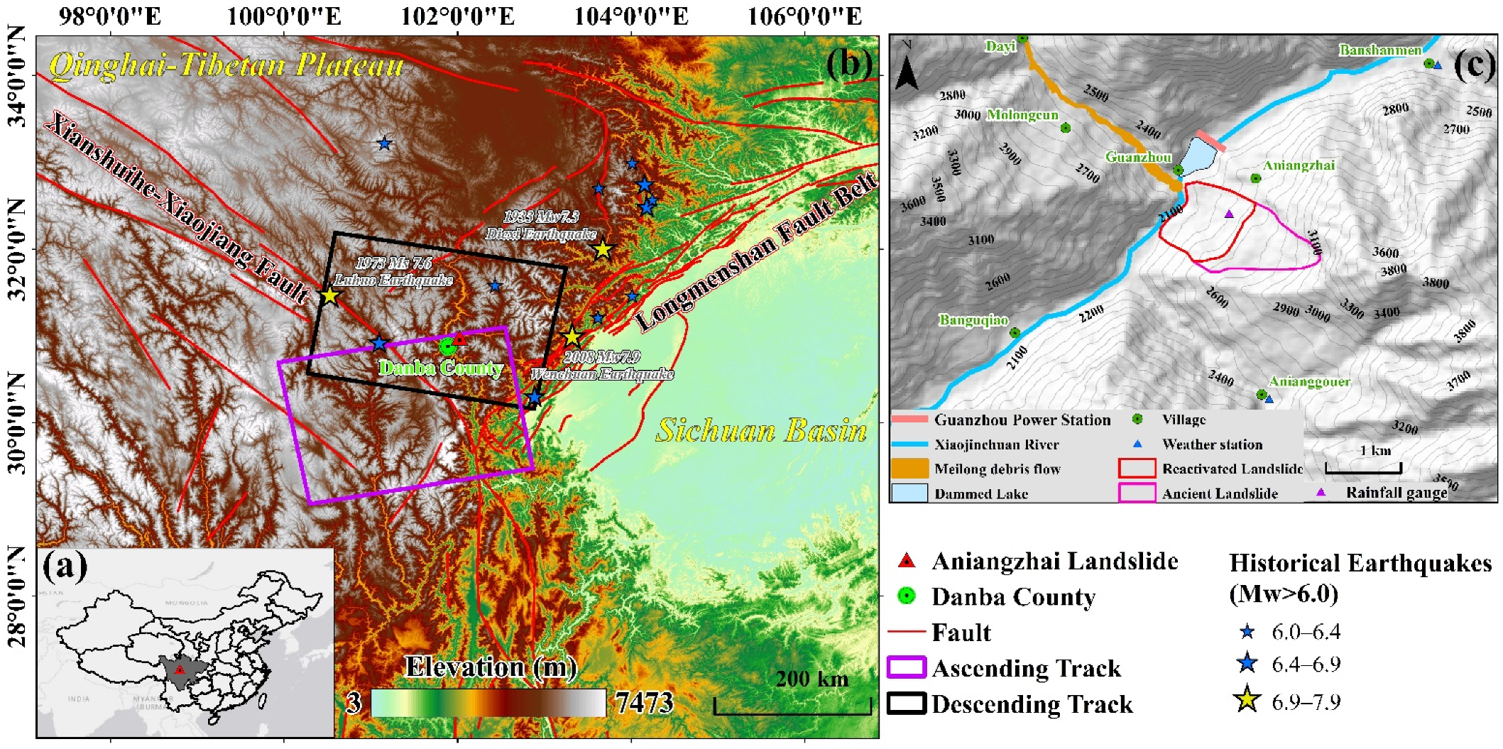
2. Study Area
3. Materials and Methods
3.1. Datasets
3.1.1. Optical Images
3.1.2. Satellite SAR Datasets
3.1.3. Rainfall Data
3.2. Optical Analysis Method
3.3. Time-Series InSAR Analysis Method
4. Results
4.1. Landslide Evolution and Deformation Mapped by Optical Datasets
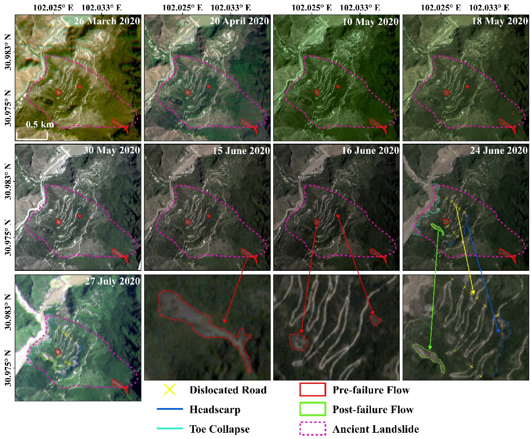
4.1.1. Landslide Evolution Revealed by the Time-Series Optical Analysis
4.1.2. Post-Failure Displacement Detected from Optical Pixel Offset Tracking
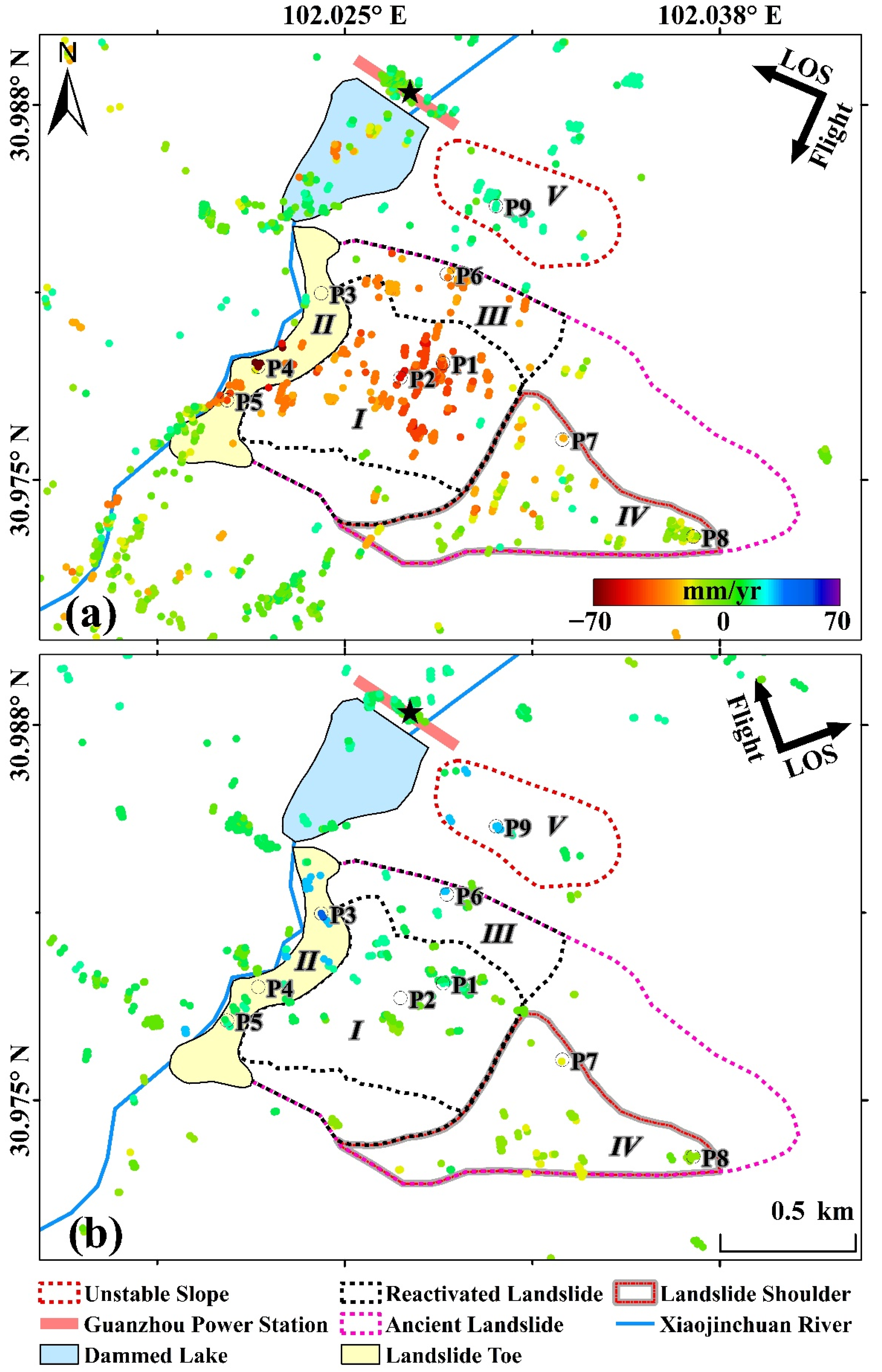
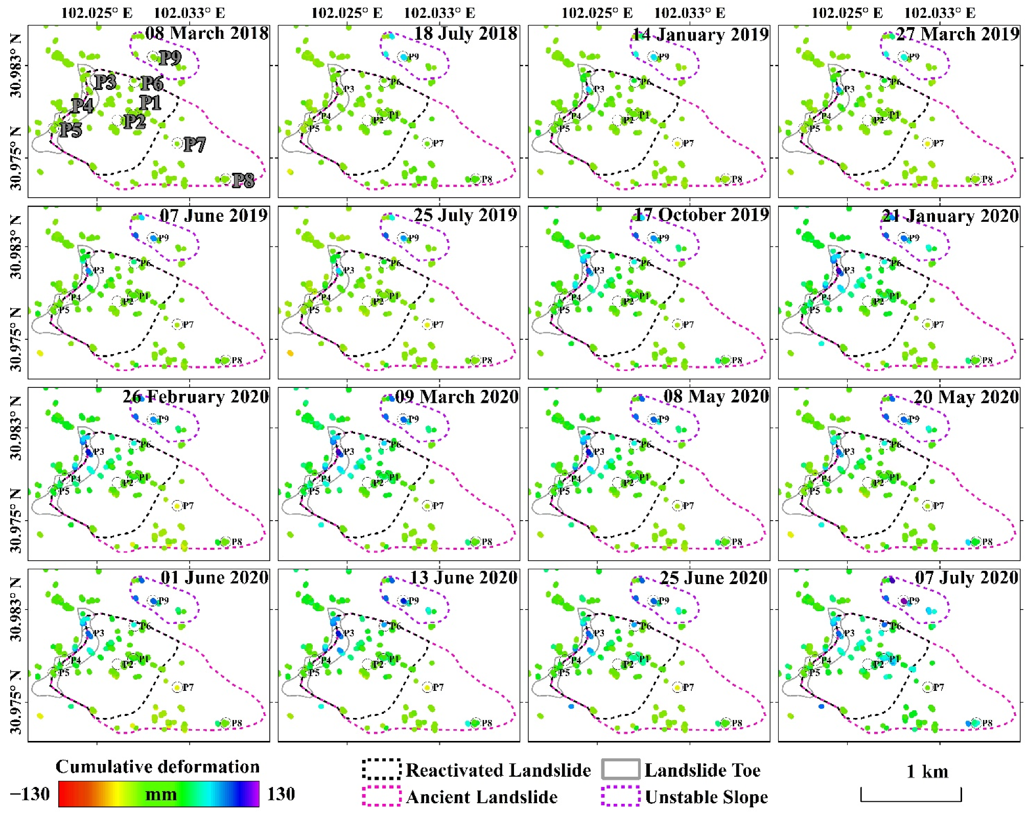
4.2. Deformation Velocity Measured by Time-Series InSAR Analysis
5. Discussion
5.1. Temporal–Spatial Evolution of the ANZ Landslide
5.2. Deformation Mechanism and Triggering/Preparatory Factor Analysis
6. Conclusions
Author Contributions
Funding
Acknowledgments
Conflicts of Interest
References
- Cruden, D.M. A simple definition of a landslide. Bull. Eng. Geol. Environ. 1991, 43, 27–29. [Google Scholar] [CrossRef]
- Sato, H.; Harp, E. Interpretation of earthquake-induced landslides triggered by the 12 May 2008, M7. 9 Wenchuan earthquake in the Beichuan area, Sichuan Province, China using satellite imagery and Google Earth. Landslides 2009, 6, 153–159. [Google Scholar] [CrossRef]
- Ren, Z.; Zhang, Z.; Yin, J. Erosion associated with seismically-induced landslides in the middle Longmen Shan region, eastern Tibetan plateau, China. Remote Sens. 2017, 9, 864. [Google Scholar] [CrossRef] [Green Version]
- Patton, A.I.; Rathburn, S.L.; Capps, D.M. Landslide response to climate change in permafrost regions. Geomorphology 2019, 340, 116–128. [Google Scholar] [CrossRef]
- Park, H.-J.; Jang, J.-Y.; Lee, J.-H. Physically based susceptibility assessment of rainfall-induced shallow landslides using a fuzzy point estimate method. Remote Sens. 2017, 9, 487. [Google Scholar] [CrossRef] [Green Version]
- Dong, J.; Zhang, L.; Li, M.; Yu, Y.; Liao, M.; Gong, J.; Luo, H. Measuring precursory movements of the recent Xinmo landslide in Mao County, China with Sentinel-1 and ALOS-2 PALSAR-2 datasets. Landslides 2018, 15, 135–144. [Google Scholar] [CrossRef]
- Fan, X.; Tang, J.; Tian, S.; Jiang, Y. Rainfall-induced rapid and long-runout catastrophic landslide on July 23, 2019 in Shuicheng, Guizhou, China. Landslides 2020, 17, 2161–2171. [Google Scholar] [CrossRef]
- Yang, Z.; Li, Z.; Zhu, J.; Preusse, A.; Yi, H.; Hu, J.; Feng, G.; Papst, M. Retrieving 3-D large displacements of mining areas from a single amplitude pair of SAR using offset tracking. Remote Sens. 2017, 9, 338. [Google Scholar] [CrossRef] [Green Version]
- Laimer, H.J. Anthropogenically induced landslides—A challenge for railway infrastructure in mountainous regions. Eng. Geol. 2017, 222, 92–101. [Google Scholar] [CrossRef]
- García-Ruiz, J.M.; Beguería, S.; Arnáez, J.; Sanjuán, Y.; Lana-Renault, N.; Gómez-Villar, A.; Álvarez-Martínez, J.; Coba-Pérez, P. Deforestation induces shallow landsliding in the montane and subalpine belts of the Urbión Mountains, Iberian Range, Northern Spain. Geomorphology 2017, 296, 31–44. [Google Scholar] [CrossRef]
- Ahmed, B.; Dewan, A. Application of bivariate and multivariate statistical techniques in landslide susceptibility modeling in Chittagong City Corporation, Bangladesh. Remote Sens. 2017, 9, 304. [Google Scholar] [CrossRef] [Green Version]
- Jingtao, L.; Yuliang, C.; Jun, W.; Youming, W.; Bin, L.; Meng, W.; Lei, Y. Remote sensing investigation and formation mechanism on wulipo landslide of July 10, 2013 in Sanxi village, Dujiangyan, Sichuan province. J. Eng. Geol. 2014, 22, 1194–1203. [Google Scholar]
- Chen, X.-Z.; Cui, Y.-F. The formation of the Wulipo landslide and the resulting debris flow in Dujiangyan City, China. J. Mt. Sci. 2017, 14, 1100–1112. [Google Scholar] [CrossRef]
- Fan, X.; Xu, Q.; Scaringi, G.; Dai, L.; Li, W.; Dong, X.; Zhu, X.; Pei, X.; Dai, K.; Havenith, H.-B. Failure mechanism and kinematics of the deadly June 24th 2017 Xinmo landslide, Maoxian, Sichuan, China. Landslides 2017, 14, 2129–2146. [Google Scholar] [CrossRef]
- Malet, J.-P.; Maquaire, O.; Calais, E. The use of Global Positioning System techniques for the continuous monitoring of landslides: Application to the Super-Sauze earthflow (Alpes-de-Haute-Provence, France). Geomorphology 2002, 43, 33–54. [Google Scholar] [CrossRef] [Green Version]
- Jaboyedoff, M.; Ornstein, P.; Rouiller, J.-D. Design of a geodetic database and associated tools for monitoring rock-slope movements: The example of the top of Randa rockfall scar. Nat. Hazards Earth Syst. Sci. 2004, 4, 187–196. [Google Scholar] [CrossRef] [Green Version]
- Squarzoni, C.; Delacourt, C.; Allemand, P. Differential single-frequency GPS monitoring of the La Valette landslide (French Alps). Eng. Geol. 2005, 79, 215–229. [Google Scholar] [CrossRef]
- Bamler, R.; Hartl, P. Synthetic aperture radar interferometry. Inverse Probl. 1998, 14, R1–R54. [Google Scholar] [CrossRef]
- Gabriel, A.K.; Goldstein, R.M.; Zebker, H.A. Mapping small elevation changes over large areas: Differential radar interferometry. J. Geophys. Res. Solid Earth 1989, 94, 9183–9191. [Google Scholar] [CrossRef]
- Massonnet, D.; Feigl, K.L. Radar interferometry and its application to changes in the Earth’s surface. Rev. Geophys. 1998, 36, 441–500. [Google Scholar] [CrossRef] [Green Version]
- Rosen, P.A.; Hensley, S.; Joughin, I.R.; Li, F.; Madsen, S.N.; Rodriguez, E.; Goldstein, R.M. Synthetic aperture radar interferometry. IOP Sci. 1998, 14, R1. [Google Scholar] [CrossRef]
- Simons, M.; Rosen, P. Interferometric synthetic aperture radar geodesy. In Treatise on Geophysics—Geodesy; Elsevier: Amsterdam, The Netherlands, 2007; pp. 391–446. ISBN 9780444527486. [Google Scholar]
- Ferretti, A.; Prati, C.; Rocca, F. Permanent scatterers in SAR interferometry. IEEE Trans. Geosci. Remote Sens. 2001, 39, 8–20. [Google Scholar] [CrossRef]
- Berardino, P.; Fornaro, G.; Lanari, R.; Sansosti, E. A new algorithm for surface deformation monitoring based on small baseline differential SAR interferograms. IEEE Trans. Geosci. Remote Sens. 2002, 40, 2375–2383. [Google Scholar] [CrossRef] [Green Version]
- Mora, O.; Lanari, R.; Mallorqui, J.J.; Berardino, P.; Sansosti, E. A new algorithm for monitoring localized deformation phenomena based on small baseline differential SAR interferograms. In Proceedings of the IEEE International Geoscience and Remote Sensing Symposium, Toronto, ON, Canada, 24–28 June 2002; pp. 1237–1239. [Google Scholar]
- Ferretti, A.; Fumagalli, A.; Novali, F.; Prati, C.; Rocca, F.; Rucci, A. A new algorithm for processing interferometric data-stacks: SqueeSAR. IEEE Trans. Geosci. Remote Sens. 2011, 49, 3460–3470. [Google Scholar] [CrossRef]
- Zhang, J.; Zhu, W.; Cheng, Y.; Li, Z. Landslide Detection in the Linzhi–Ya’an Section along the Sichuan–Tibet Railway Based on InSAR and Hot Spot Analysis Methods. Remote Sens. 2021, 13, 3566. [Google Scholar] [CrossRef]
- Dong, J.; Liao, M.; Xu, Q.; Zhang, L.; Tang, M.; Gong, J. Detection and displacement characterization of landslides using multi-temporal satellite SAR interferometry: A case study of Danba County in the Dadu River Basin. Eng. Geol. 2018, 240, 95–109. [Google Scholar] [CrossRef]
- Shi, X.; Xu, Q.; Zhang, L.; Zhao, K.; Dong, J.; Jiang, H.; Liao, M. Surface displacements of the Heifangtai terrace in Northwest China measured by X and C-band InSAR observations. Eng. Geol. 2019, 259, 105181. [Google Scholar] [CrossRef]
- Intrieri, E.; Raspini, F.; Fumagalli, A.; Lu, P.; Del Conte, S.; Farina, P.; Allievi, J.; Ferretti, A.; Casagli, N. The Maoxian landslide as seen from space: Detecting precursors of failure with Sentinel-1 data. Landslides 2018, 15, 123–133. [Google Scholar] [CrossRef] [Green Version]
- Li, M.; Zhang, L.; Dong, J.; Tang, M.; Shi, X.; Liao, M.; Xu, Q. Characterization of pre-and post-failure displacements of the Huangnibazi landslide in Li County with multi-source satellite observations. Eng. Geol. 2019, 257, 105140. [Google Scholar] [CrossRef]
- Scaioni, M.; Longoni, L.; Melillo, V.; Papini, M. Remote sensing for landslide investigations: An overview of recent achievements and perspectives. Remote Sens. 2014, 6, 9600–9652. [Google Scholar] [CrossRef] [Green Version]
- Zhou, C.; Cao, Y.; Yin, K.; Wang, Y.; Shi, X.; Catani, F.; Ahmed, B. Landslide characterization applying Sentinel-1 images and InSAR technique: The Muyubao landslide in the three gorges reservoir area, China. Remote Sens. 2020, 12, 3385. [Google Scholar] [CrossRef]
- Ciampalini, A.; Raspini, F.; Lagomarsino, D.; Catani, F.; Casagli, N. Landslide susceptibility map refinement using PSInSAR data. Remote Sens. Environ. 2016, 184, 302–315. [Google Scholar] [CrossRef]
- Dong, J.; Zhang, L.; Tang, M.; Liao, M.; Xu, Q.; Gong, J.; Ao, M. Mapping landslide surface displacements with time series SAR interferometry by combining persistent and distributed scatterers: A case study of Jiaju landslide in Danba, China. Remote Sens. Environ. 2018, 205, 180–198. [Google Scholar] [CrossRef]
- Casson, B.; Delacourt, C.; Allemand, P. Contribution of multi-temporal remote sensing images to characterize landslide slip surface—Application to the La Clapière landslide (France). Nat. Hazards Earth Syst. Sci. 2005, 5, 425–437. [Google Scholar] [CrossRef]
- Delacourt, C.; Allemand, P.; Berthier, E.; Raucoules, D.; Casson, B.; Grandjean, P.; Pambrun, C.; Varel, E. Remote-sensing techniques for analysing landslide kinematics: A review. Bull. Soc. Géol. Fr. 2007, 178, 89–100. [Google Scholar] [CrossRef]
- Lacroix, P.; Berthier, E.; Maquerhua, E.T. Earthquake-driven acceleration of slow-moving landslides in the Colca valley, Peru, detected from Pléiades images. Remote Sens. Environ. 2015, 165, 148–158. [Google Scholar] [CrossRef]
- Wright, T.J.; Parsons, B.E.; Lu, Z. Toward mapping surface deformation in three dimensions using InSAR. Geophys. Res. Lett. 2004, 31, 1–5. [Google Scholar] [CrossRef] [Green Version]
- Zhao, B.; Zhang, H.; Hongjian, L.; Li, W.; Su, L.; He, W.; Zeng, L.; Qin, H.; Dhital, M.R. Emergency response to the reactivated Aniangzhai landslide resulting from a rainstorm-triggered debris flow, Sichuan Province, China. Landslides 2021, 18, 1115–1130. [Google Scholar] [CrossRef]
- Zhu, L.; He, S.; Qin, H.; He, W.; Zhang, H.; Zhang, Y.; Jian, J.; Li, J.; Su, P. Analyzing the multi-hazard chain induced by a debris flow in Xiaojinchuan River, Sichuan, China. Eng. Geol. 2021, 106280. [Google Scholar] [CrossRef]
- Yan, Y.; Cui, Y.; Liu, D.; Tang, H.; Li, Y.; Tian, X.; Zhang, L.; Hu, S. Seismic signal characteristics and interpretation of the 2020 “6.17” Danba landslide dam failure hazard chain process. Landslides 2021, 18, 2175–2192. [Google Scholar] [CrossRef]
- Ren, J.; Xu, X.; Zhang, S.; Yeats, R.S.; Chen, J.; Zhu, A.; Liu, S. Surface rupture of the 1933 M 7.5 Diexi earthquake in eastern Tibet: Implications for seismogenic tectonics. Geophys. J. Int. 2018, 212, 1627–1644. [Google Scholar] [CrossRef]
- Chen, X.; Zhou, Q.; Ran, H.; Dong, R. Earthquake-triggered landslides in southwest China. Nat. Hazards Earth Syst. Sci. 2012, 12, 351–363. [Google Scholar] [CrossRef] [Green Version]
- Ge, L.; Zhang, K.; Ng, A.; Dong, Y.; Chang, H.-c.; Rizos, C. Preliminary results of satellite radar differential interferometry for the co-seismic deformation of the 12 May 2008 Ms8. 0 Wenchuan earthquake. Geogr. Inf. Sci. 2008, 14, 12–19. [Google Scholar]
- Farr, T.G.; Rosen, P.A.; Caro, E.; Crippen, R.; Duren, R.; Hensley, S.; Kobrick, M.; Paller, M.; Rodriguez, E.; Roth, L. The shuttle radar topography mission. Rev. Geophys. 2007, 45, 1–33. [Google Scholar] [CrossRef] [Green Version]
- Tavakkoli Piralilou, S.; Shahabi, H.; Jarihani, B.; Ghorbanzadeh, O.; Blaschke, T.; Gholamnia, K.; Meena, S.R.; Aryal, J. Landslide detection using multi-scale image segmentation and different machine learning models in the higher himalayas. Remote Sens. 2019, 11, 2575. [Google Scholar] [CrossRef] [Green Version]
- Marta, S. Planet Imagery Product Specifications; Planet Labs: San Francisco, CA, USA, 2018; p. 91. [Google Scholar]
- Torres, R.; Snoeij, P.; Geudtner, D.; Bibby, D.; Davidson, M.; Attema, E.; Potin, P.; Rommen, B.; Floury, N.; Brown, M. GMES Sentinel-1 mission. Remote Sens. Environ. 2012, 120, 9–24. [Google Scholar] [CrossRef]
- Funk, C.; Peterson, P.; Landsfeld, M.; Pedreros, D.; Verdin, J.; Shukla, S.; Husak, G.; Rowland, J.; Harrison, L.; Hoell, A. The climate hazards infrared precipitation with stations—A new environmental record for monitoring extremes. Sci. Data 2015, 2, 150066. [Google Scholar] [CrossRef] [Green Version]
- Banerjee, A.; Chen, R.; Meadows, M.E.; Singh, R.; Mal, S.; Sengupta, D. An analysis of long-term rainfall trends and variability in the uttarakhand himalaya using google earth engine. Remote Sens. 2020, 12, 709. [Google Scholar] [CrossRef] [Green Version]
- Yang, W.; Wang, Y.; Sun, S.; Wang, Y.; Ma, C. Using Sentinel-2 time series to detect slope movement before the Jinsha River landslide. Landslides 2019, 16, 1313–1324. [Google Scholar] [CrossRef]
- Fiorucci, F.; Ardizzone, F.; Mondini, A.C.; Viero, A.; Guzzetti, F. Visual interpretation of stereoscopic NDVI satellite images to map rainfall-induced landslides. Landslides 2019, 16, 165–174. [Google Scholar] [CrossRef]
- Tanre, D.; Holben, B.N.; Kaufman, Y.J. Atmospheric correction algorithm for NOAA-AVHRR products: Theory and application. IEEE Trans. Geosci. Remote Sens. 1992, 30, 231–248. [Google Scholar] [CrossRef]
- Leprince, S.; Ayoub, F.; Klinger, Y.; Avouac, J.-P. Co-registration of optically sensed images and correlation (COSI-Corr): An operational methodology for ground deformation measurements. In Proceedings of the 2007 IEEE International Geoscience and Remote Sensing Symposium, Barcelona, Spain, 23–28 July 2007; pp. 1943–1946. [Google Scholar]
- Yang, W.; Wang, Y.; Wang, Y.; Ma, C.; Ma, Y. Retrospective deformation of the Baige landslide using optical remote sensing images. Landslides 2020, 17, 659–668. [Google Scholar] [CrossRef]
- Fattahi, H.; Agram, P.; Simons, M. A network-based enhanced spectral diversity approach for TOPS time-series analysis. IEEE Trans. Geosci. Remote Sens. 2016, 55, 777–786. [Google Scholar] [CrossRef] [Green Version]
- Hooper, A. A multi-temporal InSAR method incorporating both persistent scatterer and small baseline approaches. Geophys. Res. Lett. 2008, 35. [Google Scholar] [CrossRef] [Green Version]
- Hooper, A.; Segall, P.; Zebker, H. Persistent scatterer interferometric synthetic aperture radar for crustal deformation analysis, with application to Volcán Alcedo, Galápagos. J. Geophys. Res. Solid Earth 2007, 112, 1–21. [Google Scholar] [CrossRef] [Green Version]
- Hooper, A.; Zebker, H.A. Phase unwrapping in three dimensions with application to InSAR time series. JOSA A 2007, 24, 2737–2747. [Google Scholar] [CrossRef] [PubMed] [Green Version]
- Bekaert, D.; Walters, R.; Wright, T.; Hooper, A.; Parker, D. Statistical comparison of InSAR tropospheric correction techniques. Remote Sens. Environ. 2015, 170, 40–47. [Google Scholar] [CrossRef] [Green Version]
- Fialko, Y.; Simons, M.; Agnew, D. The complete (3-D) surface displacement field in the epicentral area of the 1999 Mw7. 1 Hector Mine earthquake, California, from space geodetic observations. Geophys. Res. Lett. 2001, 28, 3063–3066. [Google Scholar] [CrossRef] [Green Version]
- Ng, A.H.-M.; Ge, L.; Li, X.; Abidin, H.Z.; Andreas, H.; Zhang, K. Mapping land subsidence in Jakarta, Indonesia using persistent scatterer interferometry (PSI) technique with ALOS PALSAR. Int. J. Appl. Earth Obs. Geoinf. 2012, 18, 232–242. [Google Scholar] [CrossRef]
- Bayramov, E.; Buchroithner, M.; Kada, M.; Zhuniskenov, Y. Quantitative Assessment of Vertical and Horizontal Deformations Derived by 3D and 2D Decompositions of InSAR Line-of-Sight Measurements to Supplement Industry Surveillance Programs in the Tengiz Oilfield (Kazakhstan). Remote Sens. 2021, 13, 2579. [Google Scholar] [CrossRef]
- Xiong, L.; Xu, C.; Liu, Y.; Wen, Y.; Fang, J. 3D displacement field of Wenchuan Earthquake based on iterative least squares for virtual observation and GPS/InSAR observations. Remote Sens. 2020, 12, 977. [Google Scholar] [CrossRef]
- Fuhrmann, T.; Garthwaite, M.C. Resolving three-dimensional surface motion with InSAR: Constraints from multi-geometry data fusion. Remote Sens. 2019, 11, 241. [Google Scholar] [CrossRef] [Green Version]
- Colesanti, C.; Wasowski, J. Investigating landslides with space-borne Synthetic Aperture Radar (SAR) interferometry. Eng. Geol. 2006, 88, 173–199. [Google Scholar] [CrossRef]
- Du, Z.; Ge, L.; Ng, A.H.-M.; Zhu, Q.; Yang, X.; Li, L. Correlating the subsidence pattern and land use in Bandung, Indonesia with both Sentinel-1/2 and ALOS-2 satellite images. Int. J. Appl. Earth Obs. Geoinf. 2018, 67, 54–68. [Google Scholar] [CrossRef]
- Marko, K.; Tiit, H.; Peeter, T.; Volli, K. Analysis of a retrogressive landslide in glaciolacustrine varved clay. Eng. Geol. 2010, 116, 109–116. [Google Scholar] [CrossRef]
- Xia, Z.; Motagh, M.; Li, T.; Roessner, S. The June 2020 Aniangzhai landslide in Sichuan Province, Southwest China: Slope instability analysis from radar and optical satellite remote sensing data. Landslides 2021, 1–17. [Google Scholar] [CrossRef]


| Stage | Imaging Date | Sun Elevation Angle (Degree) | Sun Azimuth Angle (Degree) | Instrument |
|---|---|---|---|---|
| Pre-failure | 26 March 2020 | 55.1° | 140.7° | PS2.SD |
| 20 April 2020 | 63.3° | 131.9° | PS2.SD | |
| 10 May 2020 | 64.7° | 115.9° | PS2 | |
| 18 May 2020 | 63.1° | 108.3° | PS2 | |
| 30 May 2020 | 66.7° | 107.1° | PS2 | |
| 15 June 2020 | 66.8° | 103.1° | PS2 | |
| 16 June 2020 | 66.8° | 103.1° | PS2 | |
| Post-failure | 24 June 2020 | 69.0° | 105.5° | PS2 |
| 27 July 2020 | 58.4° | 104.2° | PSB.SD |
| Satellite | Orbit | Imaging Mode | Imaging Period | Heading Angle (°) | Incidence Angle (°) | Number of Images |
|---|---|---|---|---|---|---|
| Sentinel-1A/B | Descending | TOPS | 27 March 2018–2 July 2020 | 169.6° | 37.1° | 58 |
| Ascending | TOPS | 08 March 2018–7 July 2020 | −9.8° | 44.2° | 71 |
Publisher’s Note: MDPI stays neutral with regard to jurisdictional claims in published maps and institutional affiliations. |
© 2021 by the authors. Licensee MDPI, Basel, Switzerland. This article is an open access article distributed under the terms and conditions of the Creative Commons Attribution (CC BY) license (https://creativecommons.org/licenses/by/4.0/).
Share and Cite
Kuang, J.; Ng, A.H.-M.; Ge, L. Displacement Characterization and Spatial-Temporal Evolution of the 2020 Aniangzhai Landslide in Danba County Using Time-Series InSAR and Multi-Temporal Optical Dataset. Remote Sens. 2022, 14, 68. https://0-doi-org.brum.beds.ac.uk/10.3390/rs14010068
Kuang J, Ng AH-M, Ge L. Displacement Characterization and Spatial-Temporal Evolution of the 2020 Aniangzhai Landslide in Danba County Using Time-Series InSAR and Multi-Temporal Optical Dataset. Remote Sensing. 2022; 14(1):68. https://0-doi-org.brum.beds.ac.uk/10.3390/rs14010068
Chicago/Turabian StyleKuang, Jianming, Alex Hay-Man Ng, and Linlin Ge. 2022. "Displacement Characterization and Spatial-Temporal Evolution of the 2020 Aniangzhai Landslide in Danba County Using Time-Series InSAR and Multi-Temporal Optical Dataset" Remote Sensing 14, no. 1: 68. https://0-doi-org.brum.beds.ac.uk/10.3390/rs14010068