
Detection of Windthrown Tree Stems on UAV-Orthomosaics Using U-Net Convolutional Networks


Faculty of Forest and Environment, Eberswalde University for Sustainable Development, Schicklerstraße 5, 16225 Eberswalde, Germany
*
Author to whom correspondence should be addressed.
Remote Sens. 2022, 14(1), 75; https://0-doi-org.brum.beds.ac.uk/10.3390/rs14010075
Submission received: 12 November 2021
/
Revised: 16 December 2021
/
Accepted: 22 December 2021
/
Published: 24 December 2021
(This article belongs to the Special Issue Pattern Analysis in Remote Sensing)
Abstract
:The increasing number of severe storm events is threatening European forests. Besides the primary damages directly caused by storms, there are secondary damages such as bark beetle outbreaks and tertiary damages due to negative effects on the market. These subsequent damages can be minimized if a detailed overview of the affected area and the amount of damaged wood can be obtained quickly and included in the planning of clearance measures. The present work utilizes UAV-orthophotos and an adaptation of the U-Net architecture for the semantic segmentation and localization of windthrown stems. The network was pre-trained with generic datasets, randomly combining stems and background samples in a copy–paste augmentation, and afterwards trained with a specific dataset of a particular windthrow. The models pre-trained with generic datasets containing 10, 50 and 100 augmentations per annotated windthrown stems achieved F1-scores of 73.9% (S1Mod10), 74.3% (S1Mod50) and 75.6% (S1Mod100), outperforming the baseline model (F1-score 72.6%), which was not pre-trained. These results emphasize the applicability of the method to correctly identify windthrown trees and suggest the collection of training samples from other tree species and windthrow areas to improve the ability to generalize. Further enhancements of the network architecture are considered to improve the classification performance and to minimize the calculative costs.
1. Introduction
Wind is the most significant abiotic factor causing damage to forests in Europe [1,2,3]. Severe storm incidents result in the uprooting (windthrow/windblow) or breakage (windsnap) of trees leading to significant financial losses for forest owners [4]. In 2018, the winter storm “Friederike“ caused 17 million m³ windthrown logs in Germany [5] corresponding to 28.7% of the total annual harvests [6]. Even if the severity of the storm incidents in Europe has decreased relatively in the last 30 years, compared to the heaviest storms “Wiebke” (100 million m³, 1990) and “Lothar” (180 million m³, 1999) [7], the number of severe storm incidents is continuously rising [1]. In the last 10 years, eight storm events were included in the list of the worst storm incidents according to the damages caused in German forests [7]. The German Insurance Association (GDV) and the Potsdam Institute for Climate Impact Research (PIK) forecast that this development will continue, and the number of severe storm incidents will further increase by 50% until the end of the 21st century [8].
Primary (mechanical) damages, or even blowdowns of entire stands, directly caused by storms are followed by secondary and tertiary damages [9]. Secondary damages are mostly caused by subsequent insect outbreaks, when, e.g., bark beetles benefit from the damaged and weakened trees by increasing their reproduction rates. Additionally, abiotic factors such as fire, snow or vulnerability to additional wind damages are further sources for potential secondary damages [9]. Tertiary damages in forest operations include the loss of ecological or timber productivity due to shortened forest rotations and other long-term constraints. Further tertiary damages are negativ economic impacts caused by dropping timber market prices [9].
To minimize secondary and tertiary damages, it is crucial to extract the thrown stems as quickly as possible and to sell them on the timber market [9]. This is a logistical challenge since the amount of the thrown and damaged wood cannot be quantified easily and precisely from the ground and entering the area right after the storm event is dangerous.
The aforementioned challenges can be addressed by utilizing close range remote sensing and deep learning technologies to gain fast and reliable information for the planning and implementation of extracting operations and the disposal of the fallen timber. Therefore, we propose a method for the detection and localization of windthrown or broken stems in storm-damaged forest areas on UAV orthophotos by using U-Net convolutional networks combined with an adapted data augmentation and training strategy.
Related Research
The application of neural networks to UAV imagery in the context of environmental analysis is mostly related to land cover and land use classification, tree species classification or tree health assessment, whereas the types are convolutional neural networks (CNN) or fully convolutional networks (FCN) (together 91.2%) and recurrent neural networks (RNN, 8.8%), depending on the specific task [10].
Recent FCN applications are the classification of tree species based on high resolution UAV images with less than 1.6 cm ground sampling distance (GSD) [11]. For specific tasks such as the detection and counting of agave trees in plantations, CNN are able to reach F1-scores of 96% [12]. These tasks are also accomplished by directly segmenting 3D-point clouds with 3D-CNN [13]. Conducting the analysis of storm damages in forest ecosystems, CNN/FCN were also applied for the detection of windthrow areas on satellite imagery, for instance by Hamdi et al. [14], Kislov and Korznikov [15] and on airborne CIR images [16]. To the knowledge of the authors, there are no methods of deep learning for the detection of windthrown stems on UAV-Orthophotos that have been published.
This paper demonstrates a workflow for implementing the U-Net architecture. This technique for semantic segmentation, published by Ronneberger et al. [17], is considered state-of-the-art for addressing the problem of unbalanced classes and is often applied in medical image analysis [18]. Further adaptations are the integration of residual pathways in each layer for performance gain, called MultiResU-Net [19] and the extension to the 3rd dimension [20]. The U-Net architecture and the additional adaptations are considered particularly suitable for classification tasks that demand high accuracy in minor classes such as the detection of linear structures, for example blood vessels on the retina [21].
The U-Net architecture has already been successfully applied in environmental analyses, such as the detection of open surface mining on satellite images [22] as well as on UAV images [23] and for mapping of forest types, disturbances and degradation, e.g., in tropical rainforest environments [24,25]. Furthermore, there are several applications of the U-Net architecture in UAV image analyses: delineation and classification of tree species [26], identification of plant communities [27] and prediction of cover fraction of plant species [28]. One application of a U-Net architecture, which is similar to the application addressed in this paper, is the extraction of roads from aerial images using a U-Net extended by residual units in the encoding part of the network [29]or U-Net extended by SE-blocks highlighting only useful channels [30].
Deep learning applications heavily rely on a huge amount of training samples to prevent overfitting, but in many applications, these samples are limited [31]. A commonly used practice to overcome this limitation is data augmentation, where slightly modified copies of the available training samples are supplemented. Wei and Zou [32] used synonymous replacements of sections of the data and random insertion, deletion and swapping as augmentation strategies in text analysis. The use of generic datasets [33] and copy–paste approaches [34] can also improve classification results while minimizing the effort associated with manually delineating and annotating training images. Besides the target of efficiency gain, there are also other approaches to prevent overfitting such as random erasing [35]. In medical applications even more sophisticated methods such as style transfer augmentations have been developed [36].
2. Materials and Methods
The following chapter describes the creation of the datasets used for training and validation, the adaptations of the U-Net architecture, as well as the training and evaluation strategies developed, adapted, and applied.
2.1. Investigation Area
The investigation area is located in the “East-Mecklenburg/North-Brandenburg Young Moraine Land” north-east of Berlin, Germany, which was shaped by the retreating ice masses of the Weichselian glaciation. The climatic conditions are characteristic as weakly maritime influenced lowlands [37] with an annual precipitation of 551 mm/m² and a mean annual temperature of 8.9 C [38].
The soil types of the specific windthrown area are classified as middle fine sands and the site conditions are described as “moderate fresh” without access to ground water and intermediate nutrient supply (M2) [39]. Prior to the storm event, the area was forested with 125 years old beech trees which reached a mean diameter in breast height (DBH) of 51 cm and a mean tree height in the top layer (top height) of 32 m [40].
On 5 October 2017, an area of 7.8 ha was heavily affected by the storm “Xavier”, which developed gusts reaching wind speeds up to 118 km/h and precipitation values of 55 mm/m² [41]. The storm uprooted 560 beech trees including their entire root plates that could not withstand the heavy wind speed due to the sandy soils being drenched with water.
2.2. Workflow
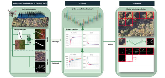
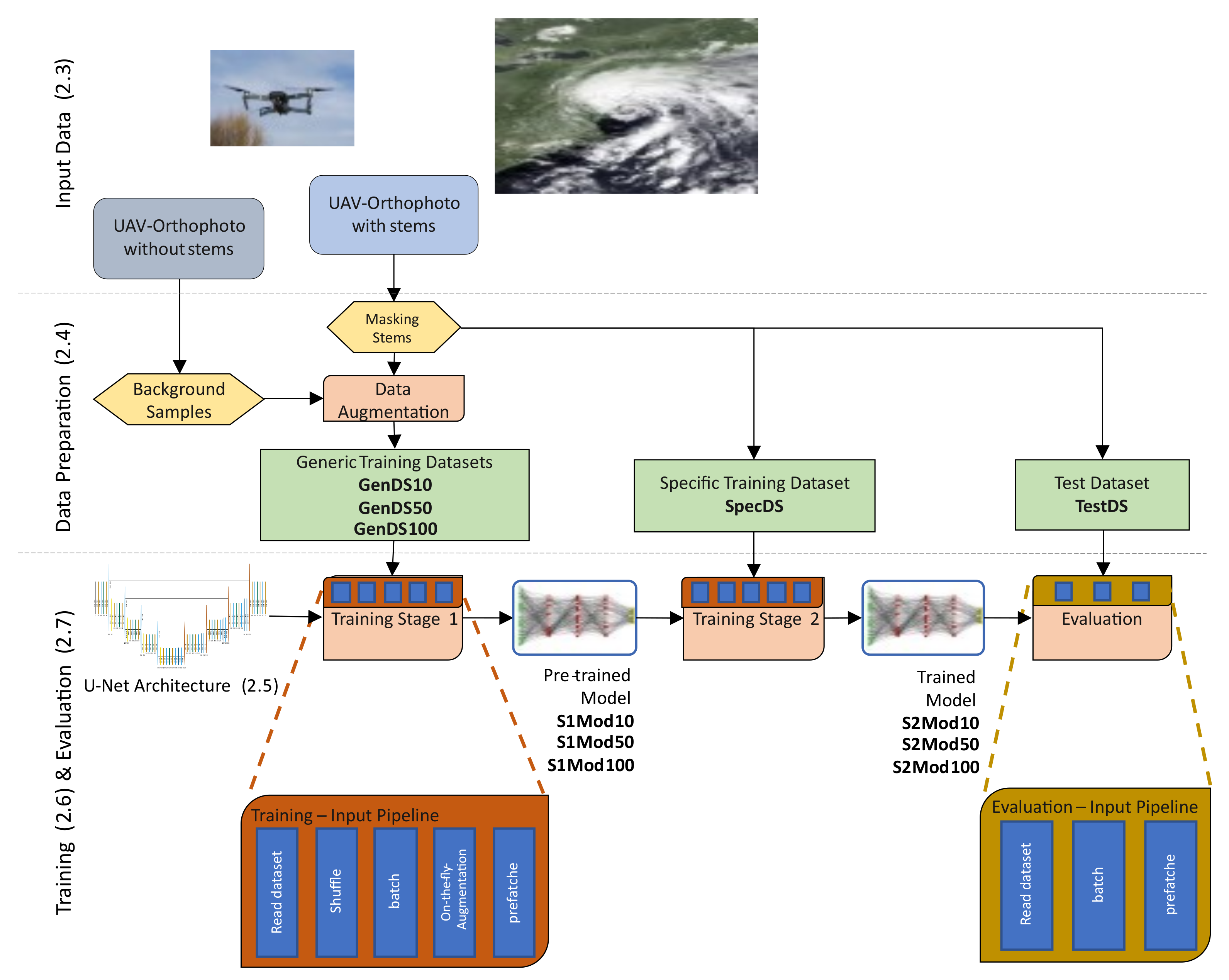
The workflow illustrated in Figure 1 can be divided in 3 parts: The acquisition of the input data using a UAV and the generation of Orthophotos (Section 2.3), the preparation of the datasets for training, validation and testing (Section 2.4) and the training and evaluation of the neural network (Section 2.6 and Section 2.7). In Section 2.5, the applied network architecture is described in detail.
2.3. UAV-Orthophotos and Extraction of the Raw Input Data
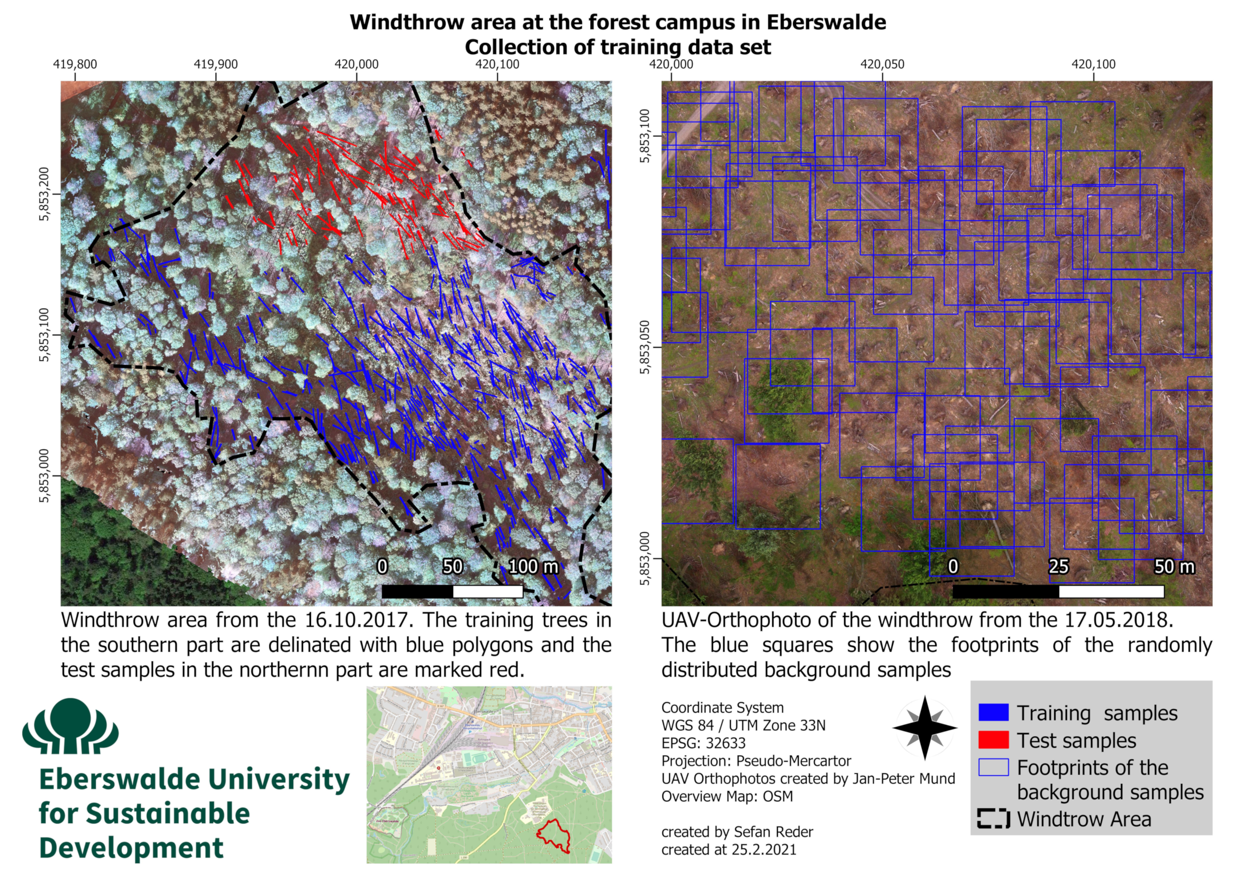
The windthrow area was captured utilizing a DJI Phantom 3 on 16 October 11 days after the storm event took place. The resulting orthophoto with a ground sampling distance (GSD) of 6.2 cm provides a sufficient resolution to visually detect the windthrown stems, even if they are partially covered by other fallen trees or tree crowns of standing trees. All 560 thrown trees were manually delineated by digitizing polygon outlines. A total of 454 trees selected from the southern and western part of the windthrow area were used for training and validation. The remaining 106 stems distributed on the northern part of the area were used as test dataset for the evaluation. A second orthophoto was taken on 17th of May, after the damaged trees had been removed, and 100 randomly distributed squared image tiles with side length of 20 m were clipped as background samples for the data augmentation (Figure 2). The reason for utilizing orthomosaics instead of the raw UAV-images is that geo-referenced images allow for an exact location and, in the post-processing, a quantification of the detected stems.
2.4. Data Preparation
In the following section, the generation of the applied datasets for training and evaluation is described. Three different types of datasets were prepared and named according to their properties and use-case:
- In training stage 1, datasets are used to train the general spectral and morphological features of single windthrown stems. Therefore, a sophisticated data augmentation strategy was applied creating slightly different copies of each stem and combining them with a random background. The resulting training datasets are called generic training datasets, hereinafter.
- In training stage 2, training samples were used that showed a particular windthrow situation, for learn the arrangement of the stems and their dimensions, called specific training dataset. No data augmentation was applied while creating this dataset.
- For the evaluation, independently collected test samples were used, hereafter called the test dataset.
An overview of the created datasets and their properties is provided in Table 1, followed by a detailed description of the creation of the listed datasets.
In order to create generic training datasets which generally represent the properties of windthrown stems instead of overfitting to the 454 samples used for training and validation, slightly different copies for each stem were created in a data augmentation process. The creation of this generic training dataset, illustrated in Figure 3 was based on two different image augmentation strategies. A copy–paste augmentation [34] was combined with classical image transformation methods. First, the clipped trees (A1) were randomly flipped, rotated and resized (max + 30%) (A2). Afterwards, brightness, saturation, contrast and hue modulations (BSCH) were applied with random values between +20% and −20% (A3). The same modulations were applied to randomly selected background samples (B1 and B2), prior to combining both samples (C). Finally, a binary training mask was created (D).
Three generic data sets (GenDS10, GenDS50 and GenDS100) were generated with 10, 50 and 100 augmented samples per tree.
In addition to the generic datasets, a specific training dataset (SpecDS) with 454 samples was created (E) by intersecting the polygons of the sample stems with square tiles (20 m × 20 m) around the centroid of each stem.
Analogously, a test dataset (TestDS) was created with 106 test samples located in the southern part of the windthrow area (Figure 2, red stems).
2.5. Network Architecture of the Adapted U-Net
The U-Net architecture introduced by Ronneberger et al. [17] was chosen for the semantic classification of the windthrow images and adapted to the specific requirements (Figure 4).
The adapted U-Net architecture (Figure 4) consists of a contracting branch (encoder) and an expansive branch (decoder), distributed over 5 levels. The input layer has an extent of 256 × 256 pixels and 3 feature layers, one for each RGB channels. Each level in the encoder contains two convolutional layers with a kernel size of 3 × 3 pixels and a max pooling layer with a pool size of 2 × 2 pixels and a stride of 2 pixels. Each contracting step to the next layer doubles the number of features (64, 128, … 1024) and down-samples their resolution to 128 × 128, 64 × 64, … 8 × 8, respectively. The decoder mirrors the encoder, but the max pooling layer is replaced by a 2 × 2 convolutional layer that halves the number of features and up-samples the layer resolution, thus inverting the operation in the contracting branch, followed by a concatenation with its corresponding layer.
To achieve better performance and to fit the requirements of the training dataset, the following adaptions were applied to the architecture proposed by Ronneberger et al. [17]: after each convolutional layer, a batch normalization layer was added to speed up training time and improve the stability and the generalization capacity of the U-Net [42]. To prevent overfitting, one dropout layer with a dropout rate of 10% was implemented on each level [43].
The hidden layers contain rectified linear units (Relu) to prevent the vanishing gradient problem [44]. In the output layer, the Sigmoid activation function was used to calculate the probability of a pixel representing a tree stem [45]. In total, the network consists of 31,133,776 trainable and 13,732 non-trainable parameters.
The ADAM optimizer was chosen to fit the model, as this optimizer was designed to handle large data sets with multiple features because it is not memory demanding [46].
Since only a minority of the pixels in the sample images are representing the objects of interest (windthrown stems), the -, which only considers these objects, was used as metric for monitoring the training process [21]. It is calculated as the harmonic mean of precision and recall of the predicted class:
The loss function “Binary Cross Entropy”, suitable for binary classification tasks [47], was adapted by adding the difference between the F1-score and 1 for a better representation of the training success.
Callbacks were introduced for reduction of the learning, when the loss was stable for 2 epochs to escape learning plateaus, and for early stopping, when the loss was not improving for 3 epochs.
An input process chain was implemented including down sampling the input images to the size of 256 × 256 pixels and a second on-the-fly augmentation. In contrary to the first augmentation, which was applied while creating the training dataset, the second data augmentation step was applied to the entire image, containing BSCH randomization and a random flip and flop operation. Finally, the dataset was shuffled and afterwards filled into batches with a size of 8 samples. On-the-fly augmentation and shuffling together assure that each epoch contained additional variability and unique batches. The training processes and the input process chain were parallelized to speed up the overall training process.
2.6. Training Strategy
The proper initialization of the model weights is crucial for the training success, since poorly initialized models are likely not being able to converge, even with a sophisticated optimizer [48]. This is especially important, when only few training samples are available. One approach to address this problem is utilizing pre-trained networks and applying transfer learning from them. This is done by using the weights of the model that was already trained and adding a new output layer with a specific classification scheme for the particular task [49]. When fine-tuning the model, the weights are updated iteratively, starting from the output layer [50].
We propose a training strategy where the classification scheme is persistent, but the network is trained in 2 stages with 2 different datasets:
- The models were pre-trained with extensive generic training datasets (GenDS10, GenDS50 and GenDS100) to train low level features on single stems.
- Afterwards, the pre-trained models were trained with the SpecDS to learn high level features, such as the pattern of several windthrown stems arranged by the storm and to fine tune the weights to the particular appearance of the stems, as the SpecDS was created without any data augmentation which morphologically or spectrally manipulates data.
2.7. Evaluation
In order to evaluate the influence of the number of augmented samples per stem of the generic training datasets (GenDS10, GenDS50 and GenDS100), the F1-score and the time to train the resulting models (S1Mod10, S1Mod50 and S1Mod100) was compared after the first training step (see above).
For the evaluation of the classification performance and the ability to generalize, the second training step was applied to the pre-trained models (S1Mod10, S1Mod50 and S1Mod100) and, in addition, a baseline model was trained only with the SpecDS dataset. Afterwards, the test data was predicted with the resulting models (Baseline, S2Mod10, S2Mod50 and S2Mod100), and the F1-scores were compared. Furthermore, 4 randomly selected tiles were visualized and interpreted.
2.8. Inference
A fishnet grid with a side length of 20 m was created to generate prediction of entire orthomosaics. The fishnet was used together with a sliding window to generate predictions of individual tiles. These predictions were subsequently merged to integrate a complete orthomosaic.
2.9. Hardware and Software Environment
As hardware environment, an Intel Xeon 5218R with 64 GB RAM and a NVIDIA Quadro RTX 5000 16 GB VRAM was used with Ubuntu 18.04.5 as operating system, CUDA driver version 11.4 and R version 4.0.4. For the implementation, the AI frameworks Keras 2.3.0 and TensorFlow 2.5 were used.
3. Results
In the following, the results of the two training stages and the classification of the test data set are presented and evaluated regarding the size of the dataset and the ability to predict independent evaluation data.
3.1. Training Stage 1
The results of the first training stage are shown in Table 2. In all cases, the networks converge, and the early stopping callback was executed automatically after 24, 20 and 22 epochs for the datasets GenDS10, GenDS50 and GenDS100, respectively. The training time per epoch increased from 2 min 31 s for the data set GenDS10 to 19 min 39 s for the data set GenDS100, which stopped after a total training time of 7:12:23 h. The training with the datasets GenDS10 and GenDS50 was proportionally shorter with 1:00:43 h and 4:12:23 h, respectively.
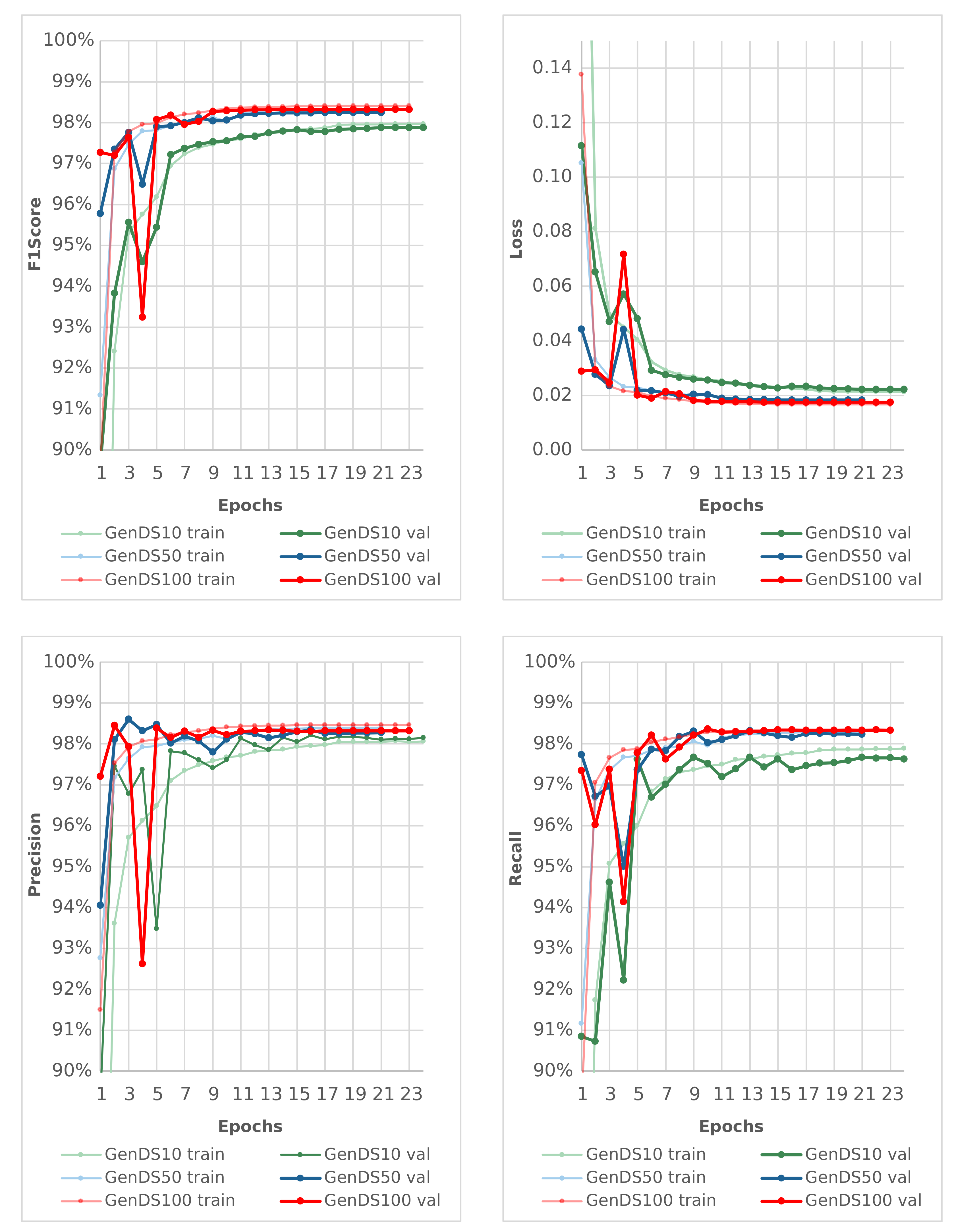
The training and validation metrics plotted in Figure 5, show that the S1Mod100 almost reach their final F1-score after nine epochs, while the S1Mod10 (F1-score 97.9, epoch 21) converges much slower with lower F1Scores. The S1Mod100 (F1-score 98.3, epoch 19) dataset shows only a little performance advantage compared with the S1Mod50 (F1-score 98.2%, epoch 21), but shows a smoother learning curve with fewer and smaller drops, especially when comparing the precision and recall curves after the first five epochs.
3.2. Training Stage 2
After applying the second training stage, the classification performance was evaluated again. The training time per epoch was nearly identical for all datasets (Table 3), but the epochs needed for convergence differed: The pre-trained models S2Mod10, S2Mod50 and S2Mod100 stopped early after 27 epochs, 32 epochs and 27 epochs with a training time of 6:54 min, 8:24 min and 6:55 min, respectively. The baseline model, which was only trained with the SpecDS, stopped after 31 epochs and a training time of 8 min 59 s.
The training is illustrated in Figure 6 on the next page. In contrary to the first training step, the pre-trained model with the most augmentations per stem (S2Mod100) reached the lowest F1-score on the validation data with 72.4% (F1-train score 74.3 ). The S2Mod50 reached a F1-validation score of 74.1% (F1 train score 74.9%) and the S2Mo10 stopped with 74.8% (F1 train 79.2%). The baseline model, which was only trained with the SpecDS dataset, reached a F1-validation score of 81.1%, but with the biggest difference to the F1-training score of 89.9%, which was still increasing when the early stopping event was triggered. This difference is an indicator for overfitting of the model on the training data.
When comparing the curves for precision and recall (Figure 6), it can be observed that the baseline model shows the roughest curves with the biggest changes in the first five epochs, and even afterwards, the curves remain unstable and show the biggest changes from one epoch to another. In contrary, the curves of pre-trained models (S2Mod10, S2Mod50 and S2Mod100) are smother and converge faster. The fastest convergence and the smoothest learning curve were observed for the S2Mod100, the model which was trained with the highest number of augmented samples per stem in the first training stage.
3.3. Evaluation
After finishing the training process, the trained models were used to classify the test dataset. The results can be seen in Table 4. The baseline model, which was trained only with the SpecDS, reached the lowest F1-score with 72.6% and also showed the lowest recall (74.2%) and precision (71.8%). The pre-trained models S2Mod10, S2Mod50 and S2Mod100 reached F1-scores of 73.9%, 74.3% and 75.6%. Furthermore, the values for precision and recall analogously rise with the number of augmented samples in the first training stage (Precision: 73.3% (S1Mod10), 73.9% (S2Mod50), 74.5% (S2Mod100); Recall: 73.5% (S2Mod10), 74.7% (S2Mod50), 76.7% (S2Mod100)).
In the following pages, Figure 7, Figure 8, Figure 9 and Figure 10 present a visual interpretation of the classification results, which illustrate the differences in classification performance between the compared models. Detailed interpretations are given in the image descriptions. Visual interpretations of the first training stage can be found in the Appendix A Figure A1, Figure A2 and Figure A3.
3.4. Inference of Orthomosaics
The model S2Mod100 was used to generate inference over complete orthomosaics, shown in Figure 11, Figure 12 and Figure 13. The orthomosaics show three different windthrow events. Figure 11 shows an area from the same site used in the model training. The orthomosaic in Figure 12 shows a nearby area not included in the training, but caused from the same storm (Xavier, 2017). The orthomosaic in Figure 13 shows a view of the area 4 years after the event. The light conditions and vegetation coverage are notably different from the images used for training, but the trained model was still able to identify most of the lying stems (bottom pane).
To generate inference in these orthomosaics, the model was fed with individual cropped images selected using a fish net as described in Section 2.8. The model output images were thereafter integrated in a mosaic to generate the bottom panes shown in Figure 11, Figure 12 and Figure 13.
4. Discussion
In the following section, the results are discussed, respectively, to the different steps of the workflow and an outlook is given on further steps considered.
4.1. Training Samples
A visual interpretation of the results revealed that, independent of the used dataset, the trained networks were able to detect small stems or branches that were not masked before, as they were smaller than the threshold used for the annotation of the thrown trees. For the use-case this is not problematic, as the smaller objects and noise can be filtered out in a post-processing step. However, as this means lower precision (as consequence of false positive predictions), a higher F1Score was also prevented (as harmonic mean of precision and recall). In the same context, the presence of leafless crowns of deciduous trees in the winter season could be challenging for image classification. This problem has not been examined yet but will be addressed when specific input data is available. Since the generic datasets (GenDS10, GenDS50 and GenDS100), as well as the SpecDS and the TestDS, originate from the same windthrow area at this project state, it is not possible to make reliable statements about the ability and limits with regard to generalization. Therefore, samples from other windthrows will be included as soon as they become available. Furthermore, for each tree species, the training dataset will be extended by tree samples of different age and with different morphological properties resulting from different stand treatments. It is also aimed to include training samples from different seasons into the specific training dataset, as the surrounding of the stems is changing during the seasons, e.g., the ground vegetation and also the foliage of the fallen trees themselves. In addition to expanding the training dataset for beech, the development of training datasets for spruce and pine will be done in the scope of the project.
4.2. Augmentation Strategy
The mentioned results could be achieved, even though the background samples of the generic dataset were captured in spring 2018, while the 1st orthophoto of the windthrow was captured in October, showing the area in a different phenological state (Figure 2). This encourages the authors to follow-up on this approach. The inclusion and combination of stem and background samples from different seasons is an obvious step to amplify robustness of the classification model. Completely generic backgrounds or backgrounds generated from classified ground points of UAV point clouds are also to be considered. A further consideration is the creation of a generic training dataset with several stems which is based on an augmentation strategy that replaces stems randomly. Therefore, the concepts of synonym replacement augmentation which is used in text classification [32] and style transfer [36] will be adapted. To improve the generalization ability while preventing overfitting, it is also under consideration to integrate random erasing in the training augmentation [35].
4.3. Training Strategy
Comparing the performance of the baseline model and the pre-trained models in the second training stage Figure 6 suggests that a proper initialized model has a lower tendency to overfitting, especially when trained with only few training samples. Furthermore, the approach of using pre-trained models with massive generic training datasets and applying only few specific training samples in a later stage, offers the opportunity for end-users without access to advanced calculative power, to fit the pre-trained model to specific windthrow incidents without huge demand for annotated images. These assumptions are backed by Pires de Lima and Marfurt [49], who demonstrated that the use of pre-trained models, based on generic training data, can outperform models trained with natural training data and create more robust models. Both aspects, the lower demand of calculative power for the final model fitting and the need for annotating only a few samples, meet the requirements of the forestry sector, where calculative power as well as personal for annotation are limited.
4.4. Network Architecture
The full classification performance of the proposed architecture has not yet been discovered and further adaptations are required. With respect to the computational costs associated with a higher resolution of the input layer, the implementation of residual layers is planned to increase the training efficiency [19,29]. Additionally, the implementation of self-calibrated convolution [51] is considered. Finally, regarding the final task of instance segmentation of the thrown stems and subsequent quantification of the wood volume and assortments of the thrown logs, the proposed architecture will be included in the mask prediction branch of a Mask-R-CNN [52].
4.5. Calculative Costs
Considerations about the computational cost are essential. In respect to limited calculation power, the images were downscaled to 256 × 256 pixel in the input chain, resulting in a GSD of 7.8 cm. For a real application in the forestry sector, such GSD is not sufficient, as longwood logs are assigned into diameter classes with a width of 4 cm [53]. To meet this requirement, the pixel size of the images should be less than half the size of the width of the diameter classes. Using images with a size of 1000 × 1000 pixels, representing a GSD of 2 cm means an upscaling of the amount of input data by the factor of 15.25. The calculative demand can be estimated with a scaling of ² to ³ [54], which means the theoretical computational costs are between 232 and 3550 times higher at this resolution. This problem must be addressed on an architectural level to keep it at the lower boundary.
5. Conclusions
In this study, we demonstrated that the proposed adaptation of the U-Net architecture as well as the combination of an appropriate augmentation and training strategy is suitable for the task of detection of windthrown tree stems on UAV-orthophotos. The pre-trained models S2Mod10, S2Mod50 and S2Mod100 achieved a F1-scores of 73.9%, 74.3% and 75.6%. The visual interpretation of the classification results suggests that a higher F1-score was not achieved because the models already detect more stem pixels correctly as masked in the training data. Above all, the ability to detect and localize single thrown trees due to the utilization of close-range remote sensing combined with deep learning is highly relevant for the forestry sector, as this provides a tool to minimize secondary damages (e.g., due to bark-beetle outbreaks). Further enhancements of the network architecture as well as the training data are considered with the aim to improve the classification performance (Section 4.1 and Section 4.4) and the ability to generalize (Section 4.1 and Section 4.2) and to minimize the calculative costs (Section 4.4 and Section 4.5).
Author Contributions
Conceptualization, S.R.; Data curation, L.W.; Funding acquisition, J.-P.M.; Investigation, S.R.; Methodology, S.R.; Project administration, J.-P.M. and N.A.; Software, S.R.; Supervision, J.-P.M. and L.M.; Validation, L.M.; Visualization, S.R.; Writing—original draft, S.R.; Writing—review and editing, J.-P.M., N.A., L.W. and L.M. All authors have read and agreed to the published version of the manuscript.
Funding
The presented work is part of the project WINMOL, a joint project of the Eberswalde University for Sustainable Development and the Thünen Institute of Forest Ecosystem Eberswalde, funded by the FNR Fachagentur für Nachwachsende Rohstoffe e.V. and the Federal Ministry of Food and Agriculture, Germany (BMEL) (FNR funding number: 2220NR024A).
Data Availability Statement
The source code, the trained models, and the used datasets as well as the training protocols are available on https://github.com/StefanReder/WINMOL_segmentor, accessed on 12 November 2021.
Acknowledgments
We thank Kenney Sauve and Avery Michelini for language editing. Furthermore, we like to thank the reviewers and the editors for their valuable contribution and support.
Conflicts of Interest
The authors declare no conflict of interest. The funders had no role in the design of the study; in the collection, analyses, or interpretation of data; in the writing of the manuscript, or in the decision to publish the results.
Appendix A. Training Stage 1
Figure A1.
S1Mod10 predicted samples of the test dataset; (left): tree mask; (middle): test samples; (right): predicted result.
Figure A1.
S1Mod10 predicted samples of the test dataset; (left): tree mask; (middle): test samples; (right): predicted result.

Figure A2.
S1Mod50 predicted samples of the test dataset; (left): tree mask; (middle): test samples; (right): predicted result.
Figure A2.
S1Mod50 predicted samples of the test dataset; (left): tree mask; (middle): test samples; (right): predicted result.

Figure A3.
S1Mod100 predicted samples of the test dataset; (left): tree mask; (middle): test samples; right: predicted result.
Figure A3.
S1Mod100 predicted samples of the test dataset; (left): tree mask; (middle): test samples; right: predicted result.

References
- Forzieri, G.; Girardello, M.; Ceccherini, G.; Spinoni, J.; Feyen, L.; Hartmann, H.; Beck, P.S.; Camps-Valls, G.; Chirici, G.; Mauri, A.; et al. Emergent vulnerability to climate-driven disturbances in European forests. Nat. Commun. 2021, 12, 1081. [Google Scholar] [CrossRef]
- Safonova, A.; Guirado, E.; Maglinets, Y.; Alcaraz-Segura, D.; Tabik, S. Olive Tree Biovolume from UAV Multi-Resolution Image Segmentation with Mask R-CNN. Sensors 2021, 21, 1617. [Google Scholar] [CrossRef]
- Gardiner, B.; Schuck, A.R.T.; Schelhaas, M.J.; Orazio, C.; Blennow, K.; Nicoll, B. Living with Storm Damage to Forests; European Forest Institute Joensuu: Joensuu, Finland, 2013; Volume 3. [Google Scholar]
- Moore, J.R.; Manley, B.R.; Park, D.; Scarrott, C.J. Quantification of wind damage to New Zealand’s planted forests. For. Int. J. For. Res. 2012, 86, 173–183. [Google Scholar] [CrossRef] [Green Version]
- Schadholzanfall 2018 in Zentraleuropa. Available online: https://www.forstpraxis.de/schadholzanfall-2018-in-zentraleuropa/ (accessed on 25 February 2021).
- Land- und Forstwirtschaft, Fischerei. Forstwirtschaftliche Bodennutzung: Holzeinschlagsstatistik 2018: Fachserie 3, Reihe 3.3.1. Available online: https://www.destatis.de/DE/Themen/Branchen-Unternehmen/Landwirtschaft-Forstwirtschaft-Fischerei/Wald-Holz/Publikationen/Downloads-Wald-und-Holz/holzeinschlag-2030331187004.html (accessed on 16 March 2021).
- Die Größten Windwürfe Seit 1990. Available online: https://www.holzkurier.com/blog/groesste-windwuerfe.html (accessed on 14 March 2021).
- Herausforderung Klimawandel. Available online: https://www.gdv.de/resource/blob/22784/a2756482fdf54e7768a93d30789506b7/publikation-herausforderung-klimawandel-data.pdf (accessed on 7 November 2021).
- Gardiner, B.; Blennow, K.; Carnus, J.M.; Fleischer, P.; Ingemarsson, F.; Landmann, G.; Lindner, M.; Marzano, M.; Nicoll, B.; Orazio, C.; et al. Destructive Storms in European Forests: Past and Forthcoming Impacts; European Forest Institute: Joensuu, Finland, 2010. [Google Scholar]
- Osco, L.P.; Junior, J.M.; Ramos, A.P.M.; Jorge, L.A.d.C.; Fatholahi, S.N.; Silva, J.d.A.; Matsubara, E.T.; Pistori, H.; Gonçalves, W.N.; Li, J. A review on deep learning in UAV remote sensing. arXiv 2021, arXiv:2101.10861. [Google Scholar] [CrossRef]
- Egli, S.; Höpke, M. CNN-Based Tree Species Classification Using High Resolution RGB Image Data from Automated UAV Observations. Remote Sens. 2020, 12, 3892. [Google Scholar] [CrossRef]
- Flores, D.; González-Hernández, I.; Lozano, R.; Vazquez-Nicolas, J.M.; Hernandez Toral, J.L. Automated Agave Detection and Counting Using a Convolutional Neural Network and Unmanned Aerial Systems. Drones 2021, 5, 4. [Google Scholar] [CrossRef]
- Nezami, S.; Khoramshahi, E.; Nevalainen, O.; Pölönen, I.; Honkavaara, E. Tree species classification of drone hyperspectral and rgb imagery with deep learning convolutional neural networks. Remote Sens. 2020, 12, 1070. [Google Scholar] [CrossRef] [Green Version]
- Hamdi, Z.M.; Brandmeier, M.; Straub, C. Forest Damage Assessment Using Deep Learning on High Resolution Remote Sensing Data. Remote Sens. 2019, 11, 1976. [Google Scholar] [CrossRef] [Green Version]
- Kislov, D.E.; Korznikov, K.A. Automatic windthrow detection using very-high-resolution satellite imagery and deep learning. Remote Sens. 2020, 12, 1145. [Google Scholar] [CrossRef] [Green Version]
- Polewski, P.; Shelton, J.; Yao, W.; Heurich, M. Instance segmentation of fallen trees in aerial color infrared imagery using active multi-contour evolution with fully convolutional network-based intensity priors. arXiv 2021, arXiv:2105.01998. [Google Scholar] [CrossRef]
- Ronneberger, O.; Fischer, P.; Brox, T. U-Net: Convolutional Networks for Biomedical Image Segmentation. In Proceedings of the International Conference on Medical Image Computing and Computer-Assisted Intervention, Munich, Germany, 5–9 October 2015. [Google Scholar]
- Sarvamangala, D.; Kulkarni, R.V. Convolutional neural networks in medical image understanding: A survey. Evol. Intell. 2021, 1–22. [Google Scholar] [CrossRef]
- Ibtehaz, N.; Rahman, M.S. MultiResUNet: Rethinking the U-Net architecture for multimodal biomedical image segmentation. Neural Netw. 2020, 121, 74–87. [Google Scholar] [CrossRef]
- Çiçek, Ö.; Abdulkadir, A.; Lienkamp, S.S.; Brox, T.; Ronneberger, O. 3D U-Net: Learning dense volumetric segmentation from sparse annotation. In Proceedings of the International Conference on Medical Image Computing and Computer-Assisted Intervention, Athens, Greece, 17–21 October 2016; pp. 424–432. [Google Scholar]
- Francia, G.A.; Pedraza, C.; Aceves, M.; Tovar-Arriaga, S. Chaining a U-net with a residual U-net for retinal blood vessels segmentation. IEEE Access 2020, 8, 38493–38500. [Google Scholar] [CrossRef]
- Maxwell, A.E.; Bester, M.S.; Guillen, L.A.; Ramezan, C.A.; Carpinello, D.J.; Fan, Y.; Hartley, F.M.; Maynard, S.M.; Pyron, J.L. Semantic Segmentation Deep Learning for Extracting Surface Mine Extents from Historic Topographic Maps. Remote Sens. 2020, 12, 4145. [Google Scholar] [CrossRef]
- Giang, T.L.; Dang, K.B.; Le, Q.T.; Nguyen, V.G.; Tong, S.S.; Pham, V.M. U-Net convolutional networks for mining land cover classification based on high-resolution UAV imagery. IEEE Access 2020, 8, 186257–186273. [Google Scholar] [CrossRef]
- Wagner, F.H.; Sanchez, A.; Tarabalka, Y.; Lotte, R.G.; Ferreira, M.P.; Aidar, M.P.; Gloor, E.; Phillips, O.L.; Aragao, L.E. Using the U-net convolutional network to map forest types and disturbance in the Atlantic rainforest with very high resolution images. Remote Sens. Ecol. Conserv. 2019, 5, 360–375. [Google Scholar] [CrossRef] [Green Version]
- Wagner, F.H.; Sanchez, A.; Aidar, M.P.; Rochelle, A.L.; Tarabalka, Y.; Fonseca, M.G.; Phillips, O.L.; Gloor, E.; Aragão, L.E. Mapping Atlantic rainforest degradation and regeneration history with indicator species using convolutional network. PLoS ONE 2020, 15, e0229448. [Google Scholar] [CrossRef] [Green Version]
- Schiefer, F.; Kattenborn, T.; Frick, A.; Frey, J.; Schall, P.; Koch, B.; Schmidtlein, S. Mapping forest tree species in high resolution UAV-based RGB-imagery by means of convolutional neural networks. ISPRS J. Photogramm. Remote Sens. 2020, 170, 205–215. [Google Scholar] [CrossRef]
- Kattenborn, T.; Eichel, J.; Fassnacht, F.E. Convolutional Neural Networks enable efficient, accurate and fine-grained segmentation of plant species and communities from high-resolution UAV imagery. Sci. Rep. 2019, 9, 17656. [Google Scholar] [CrossRef] [PubMed]
- Kattenborn, T.; Eichel, J.; Wiser, S.; Burrows, L.; Fassnacht, F.E.; Schmidtlein, S. Convolutional Neural Networks accurately predict cover fractions of plant species and communities in Unmanned Aerial Vehicle imagery. Remote Sens. Ecol. Conserv. 2020, 6, 472–486. [Google Scholar] [CrossRef] [Green Version]
- Zhang, Z.; Liu, Q.; Wang, Y. Road extraction by deep residual u-net. IEEE Geosci. Remote Sens. Lett. 2018, 15, 749–753. [Google Scholar] [CrossRef] [Green Version]
- Sofla, R.A.D.; Alipour-Fard, T.; Arefi, H. Road extraction from satellite and aerial image using SE-Unet. J. Appl. Remote Sens. 2021, 15, 014512. [Google Scholar] [CrossRef]
- Shorten, C.; Khoshgoftaar, T.M. A survey on image data augmentation for deep learning. J. Big Data 2019, 6, 1–48. [Google Scholar] [CrossRef]
- Wei, J.; Zou, K. Eda: Easy data augmentation techniques for boosting performance on text classification tasks. arXiv 2019, arXiv:1901.11196. [Google Scholar]
- Taylor, L.; Nitschke, G. Improving deep learning with generic data augmentation. In Proceedings of the 2018 IEEE Symposium Series on Computational Intelligence (SSCI), Bengaluru, India, 18–21 November 2018; pp. 1542–1547. [Google Scholar]
- Ghiasi, G.; Cui, Y.; Srinivas, A.; Qian, R.; Lin, T.Y.; Cubuk, E.D.; Le, Q.V.; Zoph, B. Simple copy-paste is a strong data augmentation method for instance segmentation. In Proceedings of the IEEE/CVF Conference on Computer Vision and Pattern Recognition, Nashville, TN, USA, 19–25 June 2021; pp. 2918–2928. [Google Scholar]
- Zhong, Z.; Zheng, L.; Kang, G.; Li, S.; Yang, Y. Random Erasing Data Augmentation. Proc. AAAI Conf. Artif. Intell. 2020, 34, 13001–13008. [Google Scholar] [CrossRef]
- Mikolajczyk, A.; Grochowski, M. Data augmentation for improving deep learning in image classification problem. In Proceedings of the 2018 International Interdisciplinary PhD Workshop (IIPhDW), Piscataway, NJ, USA, 9–12 May 2018; pp. 117–122. [Google Scholar] [CrossRef]
- Hofmann, G.; Pommer, U.; Großer, K.H. Die Waldvegetation Nordostdeutschlands, 1st ed.; Eberswalder Forstliche Schriftenreihe, Landesbetrieb Forst Brandenburg: Eberswalde, Germany, 2013; Volume 54. [Google Scholar]
- Klimadaten Eberswalde. Available online: https://meteostat.net/de/place/DE-NBFT (accessed on 15 July 2021).
- LFB. Forstliche Standortskarte im Land Brandenburg (STOK): Digitale Daten der Forstlichen Standorts- und Bodenkartierung des Landes Brandenburg. Diese Geodaten Enthalten Angaben zu Substrattypen, Bodentypen, Nährkraft, Wasserhaushalt, Grundwasserstufen. Available online: https://www.brandenburg-forst.de/LFB/client/ (accessed on 8 November 2021).
- LFB. Datenspeicher Wald 2. Available online: https://dsw2.de/index.html (accessed on 8 November 2021).
- Susanne Haeseler. Sturmtief XAVIER Zieht am 5. Oktober 2017 mit Orkanböen überDeutschland. Available online: https://www.dwd.de/DE/leistungen/besondereereignisse/stuerme/20171009_sturmtief_xavier_deutschland.pdf (accessed on 20 October 2021).
- Ioffe, S.; Szegedy, C. Batch normalization: Accelerating deep network training by reducing internal covariate shift. In Proceedings of the International Conference on Machine Learning, Lille, France, 6–11 July 2015; pp. 448–456. [Google Scholar]
- Srivastava, N.; Hinton, G.; Krizhevsky, A.; Sutskever, I.; Salakhutdinov, R. Dropout: A simple way to prevent neural networks from overfitting. J. Mach. Learn. Res. 2014, 15, 1929–1958. [Google Scholar]
- Goodfellow, I.; Bengio, Y.; Courville, A. Deep Learning; MIT Press: Cambridge, MA, USA; London, UK, 2016. [Google Scholar]
- Zayegh, A.; Bassam, N. Neural Network Principles and Applications; Pearson: London, UK, 2018; Volume 10. [Google Scholar]
- Kingma, D.P.; Ba, J. Adam: A method for stochastic optimization. arXiv 2014, arXiv:1412.6980. [Google Scholar]
- Jadon, S. A survey of loss functions for semantic segmentation. In Proceedings of the 2020 IEEE Conference on Computational Intelligence in Bioinformatics and Computational Biology (CIBCB), Viña del Mar, Chile, 27–29 October 2020; pp. 1–7. [Google Scholar]
- Sutskever, I.; Martens, J.; Dahl, G.; Hinton, G. On the importance of initialization and momentum in deep learning. In Proceedings of the International Conference on Machine Learning, Atlanta, GA, USA, 16–21 June 2013; pp. 1139–1147. [Google Scholar]
- Pires de Lima, R.; Marfurt, K. Convolutional Neural Network for Remote-Sensing Scene Classification: Transfer Learning Analysis. Remote Sens. 2020, 12, 86. [Google Scholar] [CrossRef] [Green Version]
- Käding, C.; Rodner, E.; Freytag, A.; Denzler, J. Fine-tuning deep neural networks in continuous learning scenarios. In Proceedings of the Asian Conference on Computer Vision, Taipei, Taiwan, 20–24 November 2016; pp. 588–605. [Google Scholar]
- Liu, J.J.; Hou, Q.; Cheng, M.M.; Wang, C.; Feng, J. Improving convolutional networks with self-calibrated convolutions. In Proceedings of the IEEE/CVF Conference on Computer Vision and Pattern Recognition, Seattle, WA, USA, 13–19 June 2020; pp. 10096–10105. [Google Scholar]
- He, K.; Gkioxari, G.; Dollár, P.; Girshick, R.B. Mask R-CNN. In Proceedings of the IEEE International Conference on Computer Vision (ICCV), Venice, Italy, 22–29 October 2017; pp. 2961–2969. [Google Scholar]
- Forst, D.; Holz, P. (Eds.) Rahmenvereinbarung für den Rohholzhandel in Deutschland (RVR); Deutscher Forstwirtschaftsrat e.V.: Berlin, Germany, 2020. [Google Scholar]
- Thompson, N.C.; Greenewald, K.; Lee, K.; Manso, G.F. The computational limits of deep learning. arXiv 2020, arXiv:2007.05558. [Google Scholar]
Figure 1.
Workflow diagram.

Figure 2.
Windthrow area in Eberswalde. The blue stems (left) in the southern part of the windthrow area were used to create the training datasets. The red stems were used as test dataset for the evaluation of the model performance. The blue squares (right) represent the footprints of the background images used for the data augmentation.

Figure 3.
Schematic illustrations of the augmentation process of the generic training dataset. The clipped tree (A1) is manipulated with random morphological transformations (A2) and manipulations of the pixel values (A3). The same filters are applied to the background samples (B1,B2) before both were combined into a generic tree sample (C). Finally, the training mask was calculated (D). Furthermore, for the specific windthrow samples (E), stem masks were are generated (F).

Figure 4.
U-Net architecture consisting of an encoding and a decoding branch with skipping connections between the corresponding layers. The number of features is noted below the layers and the input (left) and output (right) dimensions are provided beside each layer.
Figure 4.
U-Net architecture consisting of an encoding and a decoding branch with skipping connections between the corresponding layers. The number of features is noted below the layers and the input (left) and output (right) dimensions are provided beside each layer.

Figure 5.
Training and validation performance in training stage 1 with generic training data.

Figure 6.
Training and validation performance in training stage 2 with specific training data.

Figure 7.
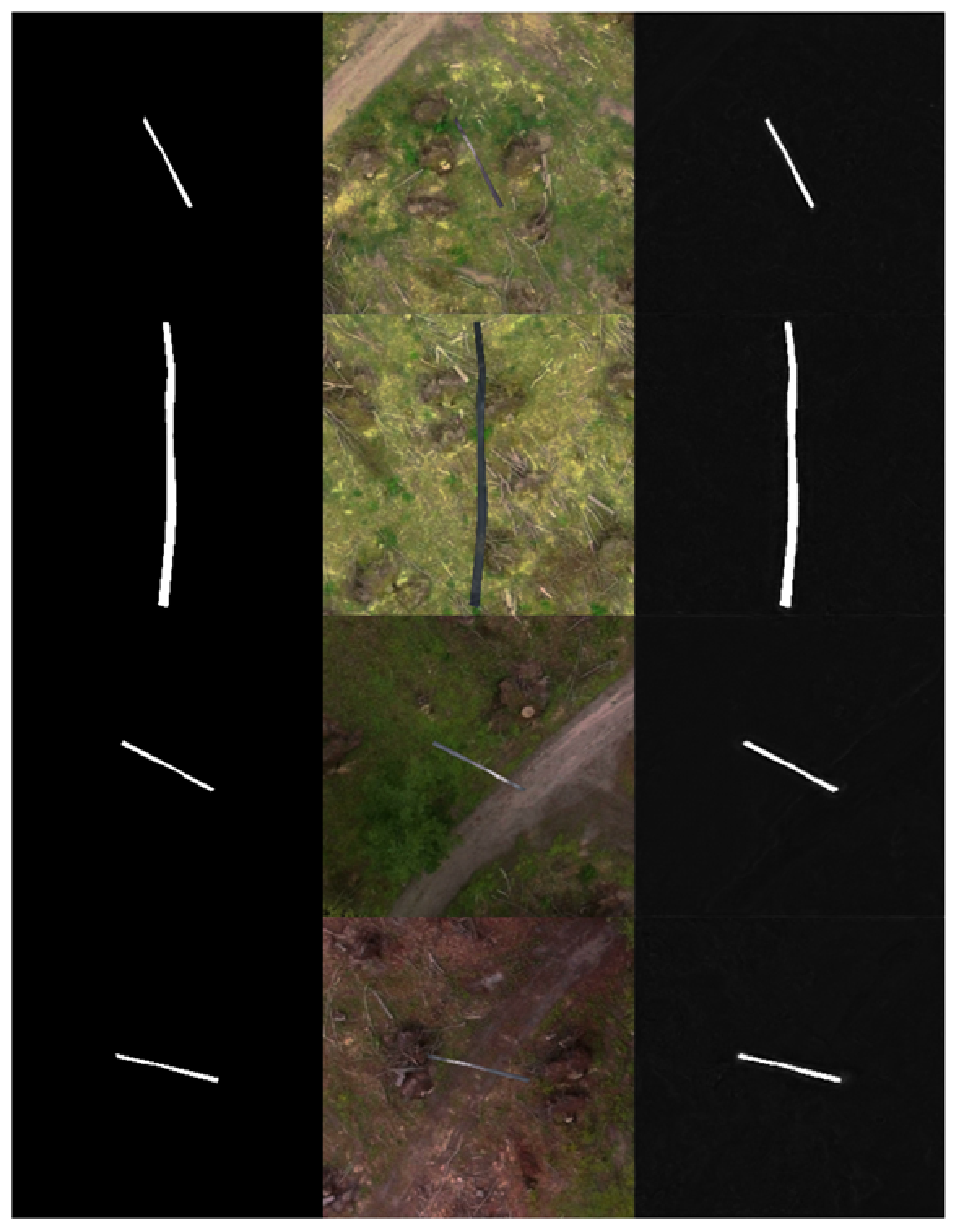
Baseline: predicted samples of the test dataset; left: tree mask; middle: test samples; right: predicted result. In some parts of the image, leaves and shadows were predicted as stem pixels (1). Smaller stems and branches, which were not masked because they were partly covered by leaves, were also detected (2). Both effects resulted in a lower precision. Furthermore, there were parts of stems which were not detected (3).
Figure 7.
Baseline: predicted samples of the test dataset; left: tree mask; middle: test samples; right: predicted result. In some parts of the image, leaves and shadows were predicted as stem pixels (1). Smaller stems and branches, which were not masked because they were partly covered by leaves, were also detected (2). Both effects resulted in a lower precision. Furthermore, there were parts of stems which were not detected (3).

Figure 8.
S2Mod10 predicted samples of the test dataset; (left): tree mask; middle: test samples; (right): predicted result. Compared to the baseline, the number of false pixels which were misinterpreted as stems pixels were reduced (1). Furthermore, the number of pixels which were detected but not present in the tree mask was increased (2). The stem parts which were not recognized in the third sample remained the same (3).

Figure 9.
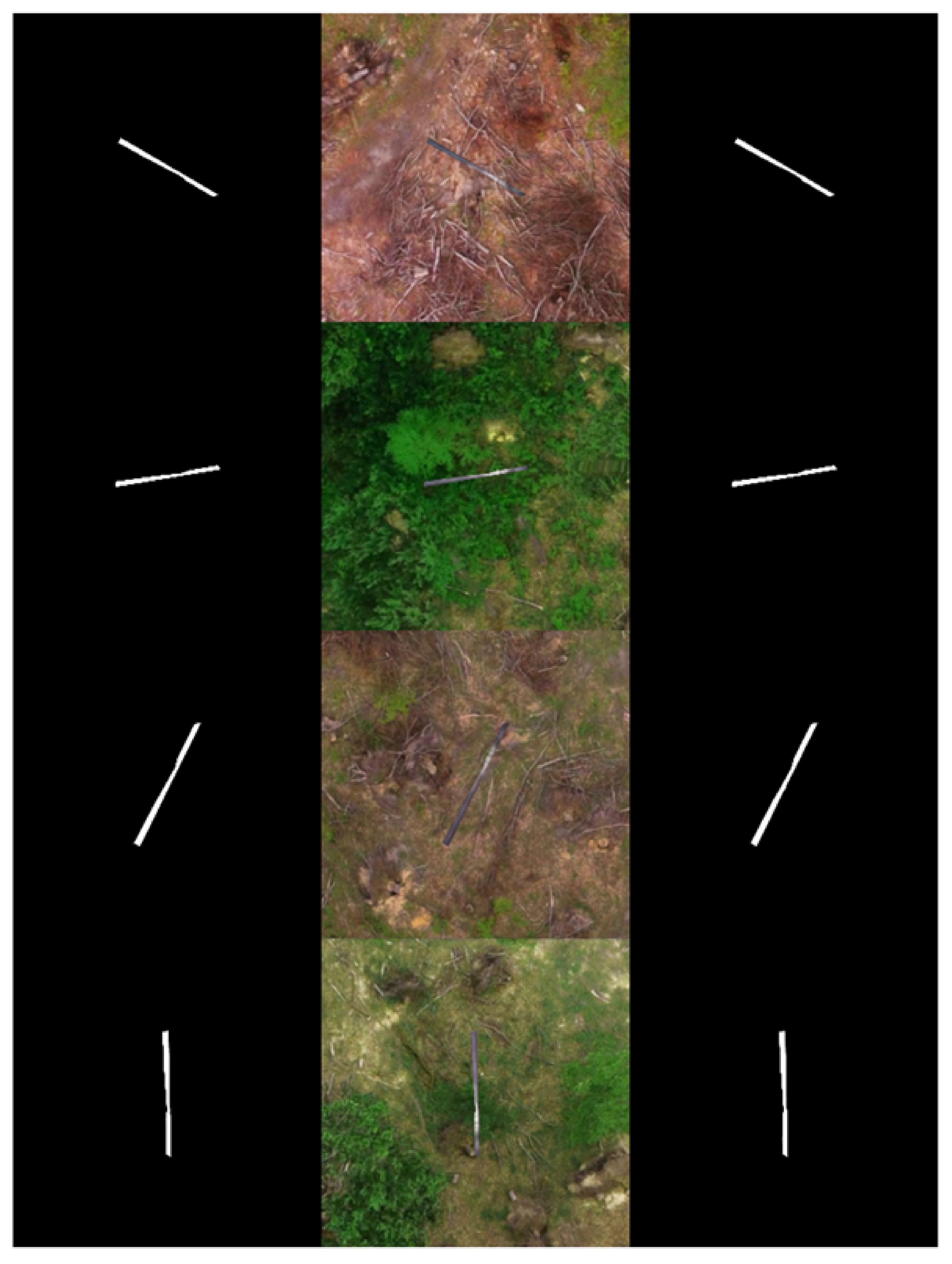
S2Mod50 predicted samples of the test dataset; left: tree mask; middle: test samples; right: predicted result. The amount of misclassified pixels stayed at the same level (1), the detected parts representing smaller branches and parts which were not masked was further increasing (2). Compared to the result of the S2Mod10 dataset, there was one additional part missing in the last sample (3).
Figure 9.
S2Mod50 predicted samples of the test dataset; left: tree mask; middle: test samples; right: predicted result. The amount of misclassified pixels stayed at the same level (1), the detected parts representing smaller branches and parts which were not masked was further increasing (2). Compared to the result of the S2Mod10 dataset, there was one additional part missing in the last sample (3).

Figure 10.
S2Mod100 predicted samples of the test dataset; (left): tree mask; middle: test samples; (right): predicted result. The result was very similar to the S2Mod50 dataset. A further improvement of the classification was visually hardly detectable. There were less misclassified pixels (1). For all models, one short part of a trunk that is partially covered by shadows was not detected (3).

Figure 11.
Orthomosaic and prediction of the training site.

Figure 12.
Orthomosaic and prediction of a damaged area close to the training site caused by the same storm event. The orhtophoto was taken on the same day. Even single thrown trees are detected between the crown openings (e.g., on the left side).
Figure 12.
Orthomosaic and prediction of a damaged area close to the training site caused by the same storm event. The orhtophoto was taken on the same day. Even single thrown trees are detected between the crown openings (e.g., on the left side).

Figure 13.
An additional windthrow area showing uprooted beech trees. The orthophoto was taken 4 years after the storm incident on the 12 August 2021. The area was captured during a different season with a different UAV (Phantom 4 RTK), the illumination is different and the trees are already decaying. Nevertheless, most of the trees are recognized.


Table 1.
Overview of the training and test datasets.
| Dataset | Sample Size | Type | Number of Stems | Data Augmentation | Utilization |
|---|---|---|---|---|---|
| GenDS10 | 4540 | generic training dataset | single | 10 per stem | training stage 1 |
| GenDS50 | 22,700 | generic training dataset | single | 50 per stem | training stage 1 |
| GenDS100 | 45,400 | generic training dataset | single | 100 per stem | training stage 1 |
| SpecDS | 454 | specific training dataset | multiple | no | training stage 2 |
| TestDS | 106 | test dataset | multiple | no | evaluation |
Table 2.
Training stage 1.
| Model | Dataset | Sample Size | Epochs | Time per Epoch | Training Time |
|---|---|---|---|---|---|
| S1Mod10 | GenDS10 | 4540 | 24 | 0:02:31 h | 1:00:43 h |
| S1Mod50 | GenDS50 | 9080 | 20 | 0:12:12 h | 4:03:52 h |
| S1Mod100 | GenDS100 | 45,400 | 22 | 0:19:39 h | 7:12:23 h |
Table 3.
Training stage 2.
| Model | Dataset | Sample Size | Epochs | Time per Epoch | Training Time |
|---|---|---|---|---|---|
| Baseline | SpecDS | 454 | 31 | 0:00:17 h | 0:08:59 h |
| S1Mod10 | SpecDS | 454 | 27 | 0:00:15 h | 0:06:54 h |
| S1Mod50 | GSpecDS | 454 | 32 | 0:00:16 h | 0:08:24 h |
| S1Mod100 | SpecDS | 454 | 27 | 0:00:15 h | 0:06:55 h |
Table 4.
Evaluation results.
| Model | Dataset | Sample Size | F1-Score | Precision | Recall |
|---|---|---|---|---|---|
| Baseline | SpecDS | 106 | 72.6% | 71.8% | 74.2% |
| S1Mod10 | SpecDS | 106 | 73.9% | 73.3% | 74.5% |
| S1Mod50 | GSpecDS | 106 | 74.3% | 73.9% | 74.7% |
| S1Mod100 | SpecDS | 106 | 75.6% | 74.5% | 76.7% |
Publisher’s Note: MDPI stays neutral with regard to jurisdictional claims in published maps and institutional affiliations. |
© 2021 by the authors. Licensee MDPI, Basel, Switzerland. This article is an open access article distributed under the terms and conditions of the Creative Commons Attribution (CC BY) license (https://creativecommons.org/licenses/by/4.0/).
Share and Cite
MDPI and ACS Style
Reder, S.; Mund, J.-P.; Albert, N.; Waßermann, L.; Miranda, L. Detection of Windthrown Tree Stems on UAV-Orthomosaics Using U-Net Convolutional Networks. Remote Sens. 2022, 14, 75. https://0-doi-org.brum.beds.ac.uk/10.3390/rs14010075
AMA Style
Reder S, Mund J-P, Albert N, Waßermann L, Miranda L. Detection of Windthrown Tree Stems on UAV-Orthomosaics Using U-Net Convolutional Networks. Remote Sensing. 2022; 14(1):75. https://0-doi-org.brum.beds.ac.uk/10.3390/rs14010075
Chicago/Turabian StyleReder, Stefan, Jan-Peter Mund, Nicole Albert, Lilli Waßermann, and Luis Miranda. 2022. "Detection of Windthrown Tree Stems on UAV-Orthomosaics Using U-Net Convolutional Networks" Remote Sensing 14, no. 1: 75. https://0-doi-org.brum.beds.ac.uk/10.3390/rs14010075
Note that from the first issue of 2016, this journal uses article numbers instead of page numbers. See further details here.