
Optimization Framework for Spatiotemporal Analysis Units Based on Floating Car Data


1
School of Geosciences, Yangtze University, Wuhan 430100, China
2
School of Computer Science, China University of Geosciences, Wuhan 430074, China
3
National Engineering Research Center of Geographic Information System, Wuhan 430074, China
*
Author to whom correspondence should be addressed.
Remote Sens. 2022, 14(10), 2376; https://0-doi-org.brum.beds.ac.uk/10.3390/rs14102376
Submission received: 22 March 2022
/
Revised: 8 May 2022
/
Accepted: 11 May 2022
/
Published: 14 May 2022
(This article belongs to the Special Issue Advances to GIS for Sensing of Earth and Human Interaction)
Abstract
:Spatiotemporal scale is a basic component of geographical problems because the size of spatiotemporal units may have a significant impact on the aggregation of spatial data and the corresponding analysis results. However, there is no clear standard for measuring the representativeness of conclusions when geographical data with different temporal and spatial units are used in geographical calculations. Therefore, a spatiotemporal analysis unit optimization framework is proposed to evaluate candidate analysis units using the distribution patterns of spatiotemporal data. The framework relies on Pareto optimality to select the spatiotemporal analysis unit, thereby overcoming the subjectivity and randomness of traditional unit setting methods and mitigating the influence of the modifiable areal unit problem (MAUP) to a certain extent. The framework is used to analyze floating car trajectory data, and the spatiotemporal analysis unit is optimized by using a combination of global spatial autocorrelation coefficients and the coefficients of variation of local spatial autocorrelation. Moreover, based on urban hotspot calculations, the effectiveness of the framework is further verified. The proposed optimization framework for spatiotemporal analysis units based on multiple criteria can provide suitable spatiotemporal analysis scales for studies of geographical phenomena.
1. Introduction
Geographical spatiotemporal big data enable us to explore urban science and obtain new insights [1]. By using the spatiotemporal big data collected with a variety of methods (e.g., global positioning systems (GPSs), global systems for mobile communication (GSMs), smart cards (SCs), and social media (SM)), researchers can observe and analyze urban problems at multiple spatiotemporal scales; such problems include traffic congestion monitoring and urban structure planning [2,3,4]. The results can provide new information for describing and understanding urban space.
Although spatiotemporal big data provide many unique advantages and opportunities for urban problem analysis, such data are also associated with notable challenges. Spatial combination is an essential analysis step when assessing the geospatial environment from personal-level geographic big data. It is usually necessary to aggregate spatiotemporal data into a spatial area according to a certain temporal unit. Areas are commonly divided into analysis units of different sizes, and the areas and shapes of these units also vary. This spatial approach for data aggregation is very sensitive to the scale and zoning effects of the modifiable areal unit problem (MAUP). Scale effects describe changes in statistical results when analyzed using data aggregated at different unit granularities. The zoning effect refers to the variability of results caused by different zoning schemes when the number of units is constant. Due to the uncertainty regarding the number (scale effect) and shape (zoning effect) of spatial units, the MAUP can lead to very different spatial patterns and statistical results [5,6].
In urban computing, when using geographical big data to reflect real-world spatiotemporal phenomena, the MAUP is usually ignored, and scale and zoning effects are rarely mentioned. However, many scholars have recently studied how to alleviate the MAUP. Jiang and Miao focused on the hierarchical agglomeration and heterogeneity of social media data to determine the corresponding urban structure, thus mitigating the statistical bias of the MAUP [7]. However, they did not evaluate the effect of the MAUP or provide a strategy for optimizing the selection of spatial analysis units. Lee et al. assessed the effect of the MAUP through the rate of change of the global spatial correlation coefficient using a regular grid of units with different areas [8]. Meng et al. proposed selecting regional analysis units based on attribute distributions to produce high global Moran’s I values in an approach similar to that used for the segmentation of high-resolution remote sensing imagery [9]. Moreover, Jelinski and Wu noted that the analysis results obtained at one scale provide incomplete information about the spatial pattern, and for any spatial analysis case, it is necessary to associate the analysis with a given spatial scale [10]. Fotheringham et al. suggested that the sensitivity of parameter estimates needs to be assessed at different spatial scales before the analysis results are provided to decision makers [11]. Based on sensitivity analysis, the influence of specific parameters on the results of statistical analysis can be quantitatively studied. Although research on the MAUP and analyses of geographical big data have proliferated, a standard solution to the MAUP has not been obtained because different geographical phenomena are generally associated with different spatiotemporal distributions.
When analyzing high-resolution geospatial-temporal datasets, the aggregation of data can be customized at various geographical levels (e.g., traffic analysis zones, grids, or street networks), thus alleviating the MAUP to some extent. However, previous studies have shown that the distributions of geographical spatiotemporal data are scale sensitive, and the interrelationships among attributes vary at different scales [12,13]. Specifically, when using area data for spatial analysis, the calculated results may be unstable or uncertain based on the selection of different analysis units, and a unified conclusion cannot be obtained. Therefore, determining the best research units for spatiotemporal data to enhance urban design and management has become an important topic.
Spatial autocorrelation (SA) is the main factor that leads to the MAUP. Many scholars have assessed the relationships between different analysis units and SA, especially how the overall structure of SA changes with different spatial units. These studies provided some solutions for dealing with the MAUP [14,15,16]. Openshaw and Fotheringham explored the relationship between SA and the MAUP and found that when spatial aggregation occurred, the data were smoothed, resulting in reductions in variance and correlation values [17,18]; that is, if adjacent spatial units are aggregated to form a larger unit and their covariance is assumed to be relatively stable, the corresponding heterogeneity decreases, resulting in reductions in the variance and correlation coefficient. In addition, since MAUP effects are associated with different levels of SA, the sensitivity to MAUP effects may also vary based on the variables considered, making it difficult to analyze MAUP effects in cases with multiple variables.
In addition, indicators used to measure SA, such as Moran’s I, are also affected by MAUP effects. Cliff and Ord found a negative correlation between spatial aggregation and SA, indicating that the larger the size of an area unit is, the smaller Moran’s I [19]. Similarly, Chou discussed the possible relationship between map resolution and Moran’s I (log-linear relationship) [14], and Qi and Wu obtained similar results from their analysis of landscape pattern data [15]. Griffith et al. showed that the SA calculated based on Moran’s I decreases with increasing spatial resolution of the analysis units [16]. In the above research, the relationships between different analysis units and SA were explored. A decrease in the variance reduces the denominator of Moran’s I, resulting in an increase in Moran’s I. Additionally, a decrease in the variance reduces the spatial covariance difference in the numerator of Moran’s I and thus reduces Moran’s I. Therefore, when the reduction in the numerator is greater than that in the denominator, Moran’s I tends to zero. In other words, different spatial analysis units lead to local SA heterogeneity, resulting in variations in Moran’s I. Consequently, the use of different spatial units generally leads to different statistical results [20]. Determining the spatial unit most suitable for spatially assessing geographical phenomena, that is, the dependence or sensitivity of geographical processes in different spatial units, is important for studies of geographical phenomena.
When using spatiotemporal travel data to assess urban problems, the selection of the most appropriate spatiotemporal analysis unit is complex. Because people’s movements in urban spaces are influenced by their daily activities at different times and are unevenly distributed, it is necessary to explore the relationships between the spatiotemporal processes that influence people’s activities and the spatiotemporal phenomena of interest [21,22]. For a certain spatial unit, the data distribution patterns vary in different time intervals; that is, the global and local spatial correlations of the data differ. Therefore, different temporal units produce different spatial distribution patterns, resulting in different spatiotemporal data analysis results [23,24]. That is, the temporal unit considered influences the spatial analysis results. Therefore, the determination of the best temporal unit should be considered in conjunction with that of the optimal spatial unit.
When analyzing urban geographical phenomena based on spatiotemporal data, different spatiotemporal analysis units are associated with different levels of uncertainty; notably, it is often unclear how to match the analysis unit to the scale of a geographical phenomenon. However, sensitivity analysis using spatially correlated global indicators is an effective method for mitigating the MAUP. This method considers only the overall aggregated pattern of spatiotemporal data, whereas the spatial differences and instabilities of local patterns are ignored. Therefore, applying the global Moran’s I alone is not sufficient for assessing the spatiotemporal heterogeneity of data, especially in study areas that are divided into many analysis units. Most global spatial correlation metrics assume that the corresponding data are characterized by spatial and temporal homogeneity, but geographic big data often have spatially and temporally discrete distributions. In addition, local spatial patterns are particularly important in urban analysis since the heterogeneity of the internal structure of a city affects data generation. Comprehensive analyses have shown that geographical big data are generally associated with a low/moderate level of spatiotemporal dependence (i.e., spatial correlation) and high spatiotemporal heterogeneity. Thus, the best spatiotemporal analysis units for geographical big data should be comprehensively considered based on different indicators.
In this paper, a data-driven approach is adopted to determine the most suitable spatiotemporal analysis unit for assessing floating vehicle trajectory data, and a multicriteria-based optimization framework for spatiotemporal analysis units is proposed to explore spatial data distribution patterns at different scales. With the Wuhan taxi trajectory dataset as an example, the data distribution patterns at multiple grid scales are aggregated, and MAUP effects are described based on global and local indicators of spatial correlation. Then, the optimal analysis unit is determined using Pareto optimality. Additionally, a sensitivity analysis of the proposed framework is performed. Finally, with the calculation of urban hotspots as an example, the validity and rationality of the optimization framework for spatiotemporal data analysis units integrating temporal and spatial scales are further verified.
2. Materials and Methods
2.1. Methodological Flow
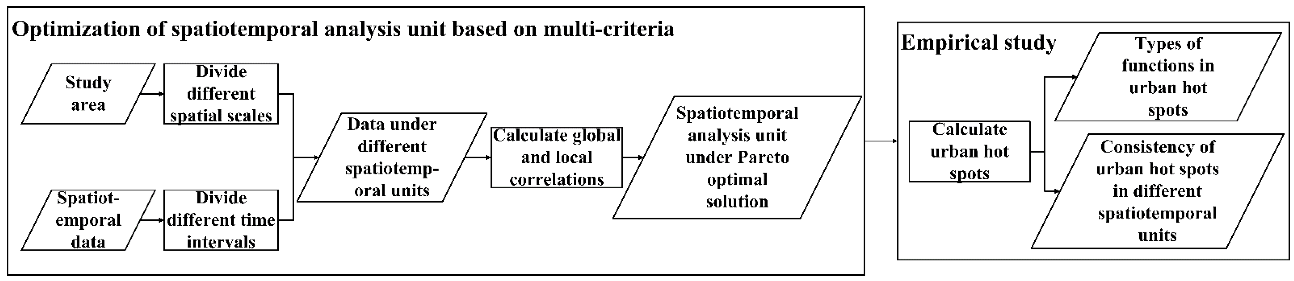
To select the appropriate spatiotemporal analysis unit when using spatiotemporal data to analyze geographic phenomena, an optimization framework for spatiotemporal analysis units is proposed based on multiple criteria (as shown in Figure 1). The optimization framework for spatiotemporal analysis units based on multiple criteria is proposed with reference to multicriteria decision analysis (MCDA) [25]. MCDA can provide a systematic and general problem-solving method for decision makers to select suitable solutions from a limited set of candidates [26,27]. The spatiotemporal data analysis unit optimization framework can select the optimal spatiotemporal analysis unit based on multiple criteria, thus providing a spatiotemporal analysis scale for studies of geographical phenomena. The technical workflow of this paper is shown in Figure 1.
According to Figure 1, the research content of this paper is divided into the following four parts.
(1) Data organization and spatiotemporal unit division
In this study, the spatiotemporal data in the study area are preprocessed to extract all available data in the corresponding spatiotemporal units. Then, based on trajectory data for floating cars, analysis units with different spatial and temporal scales are determined. Finally, the distribution of the trajectory data is obtained considering the corresponding spatiotemporal analysis units.
(2) Global and local correlation calculations
The distribution characteristics of data at different spatial and temporal scales are explored. At the same time, the data distributions are assessed using different statistical criteria. In this paper, the global Moran’s I and the coefficient of variation of local Moran’s I are combined to analyze the distributions of datasets at different spatiotemporal scales.
(3) Optimal spatiotemporal unit determination
The Pareto-optimal algorithm is used to divide the boundaries of different spatiotemporal analysis units and determine the optimal spatiotemporal analysis scale for the study area. Moreover, a location-based resampling method is applied to verify the sensitivity of the optimal spatiotemporal analysis unit.
(4) Empirical study
In this paper, scenarios involving actual geographical phenomena are used to verify the optimal spatiotemporal analysis unit. First, the locations of urban hotspots are confirmed based on the optimal spatiotemporal analysis unit, and the effectiveness of the optimization framework based on multiple criteria is verified based on the hotspot distribution and corresponding functional areas. Moreover, the effects of different spatial and temporal units on the data analysis results are assessed by using a consistency coefficient (i.e., overall kappa coefficient) for urban hotspots in different spatiotemporal units.
2.2. Study Area and Data
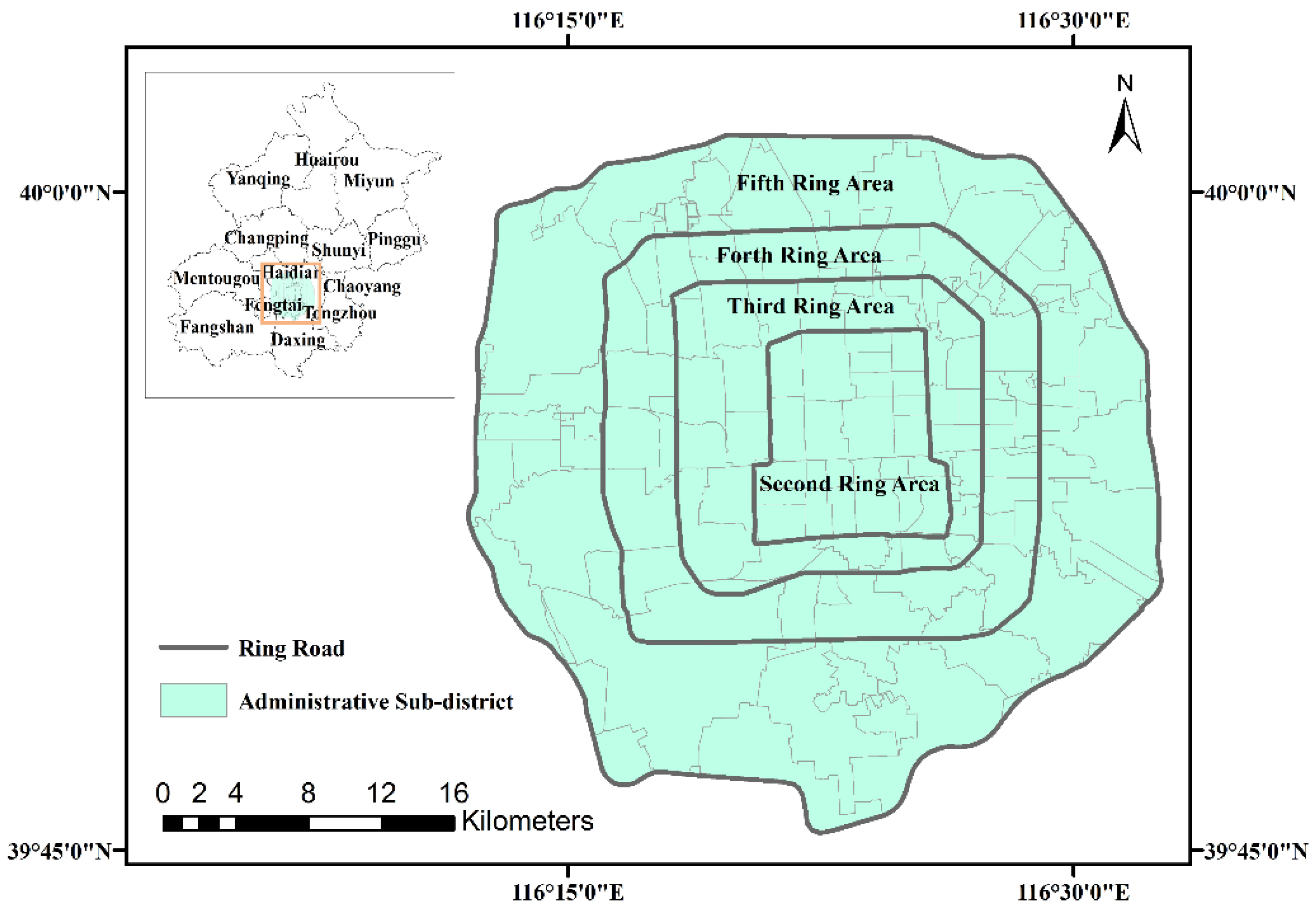
Beijing, the capital of China, is located at 39°26′N–41°03′N and 115°25′E–117°30′E. The total area is 16,410 square kilometers, the resident population is 21.89 million, and the GDP ranks first in the country. The Fifth Ring Road of Beijing is the dividing line between the urban area and the suburbs, and the urban area includes six major districts (Chaoyang District, Haidian District, Dongcheng District, Xicheng District, Shijingshan District, and Fengtai District). A map of the Second Ring Road to the Fifth Ring Road areas is shown in Figure 2. Beijing has a very convenient transportation system that includes buses, subways, and taxis. Among them, taxis transport an average of 1.9 million passengers per day, accounting for 6.6% of the total travel volume and providing comprehensive travel services for urban residents [28]. Although the area of the Fifth Ring Road in Beijing accounts for only 4% of the total area of the city, the population in this zone accounts for more than 50% of the total Beijing population, indicating that residents’ activities are mainly concentrated within the Fifth Ring Road [29]. Therefore, floating car data, which reflect the characteristics of residents’ movement behaviors, collected within Beijing’s Fifth Ring Road are used to determine the most suitable spatiotemporal analysis unit.
Taxi GPS data collected on two working days (14 and 15 November 2012) are used to explore the optimal spatiotemporal analysis unit [30]. The interval of data collection was approximately 1 min, and the entire dataset contains more than 30 million records. The experimental data were provided by the Beijing Taxi Operation Company and stored in a .txt file. The GPS point data include the taxi ID, recording time, longitude, latitude, vehicle speed, driving direction, and status (0 for empty and 1 for passenger) information, as shown in Table 1. Abnormal data in the study area were removed, and data for records with passengers were extracted.
2.3. Methods
2.3.1. Division of Spatiotemporal Units
The MCDA problem can be modelled with a two-dimensional decision matrix, where each element (a spatiotemporal analysis unit) represents a calculation result for a different criterion (column) and corresponds to a specific decision, also known as a candidate solution. The numbers of criteria and candidate solutions are unlimited; however, the number of candidates can be reduced if the elements and criteria are constrained for a certain problem. The optimization framework proposed in this paper is for spatiotemporal geographical phenomena. Therefore, selecting a series of geographically significant spatiotemporal analysis units for data analysis can narrow the range of candidate spatiotemporal analysis units for researchers.
To alleviate MAUP effects and try to eliminate the influence of different types of spatial units, a grid is adopted, and spatial analysis units of different scales are selected to study the influence of spatial scale on the data distribution. In addition, to determine the best temporal unit, the influence of temporal scale on the data distribution is analyzed by selecting temporal analysis units of different scales. The distribution of spatiotemporal data is determined at each different spatiotemporal scale, and the corresponding spatial correlations are calculated to determine the optimal spatiotemporal analysis unit according to multiple criteria.
2.3.2. Global and Local Moran’s I
According to the research content of this paper, global and local correlations are taken as the criterion of MCDA. That is, the optimal spatiotemporal analysis unit for floating car data is evaluated in terms of global spatial autocorrelation and the coefficient of variation of local correlation. The former is related to the overall spatial distribution of trajectory data, and the latter measures data instability through local inequality. The coefficient of variation is used to summarize the local spatial distribution pattern. When comparing the degree of data variation, the coefficient of variation cannot only eliminate the influence of the mean difference on the dispersion calculation, but also avoid the influence of the data of different measurement dimensions on the result evaluation.
Global and local spatial correlations are measured with the global Moran’s I and local Moran’s I. The global Moran’s I represents the overall correlation between an object and all surrounding objects, that is, the overall spatial aggregation effect of the data. The local Moran’s I expresses the correlation between an object and every surrounding object, and reflects the difference with surrounding objects. The coefficient of variation of local Moran’s I can reflect the stability of the local spatial distribution of the data.
The global spatial autocorrelation can be expressed as Equation (1).
where is the deviation in the attribute of feature i from its mean (deviation in the GPS number in spatial unit i from its mean), is the spatial weight between features i and j (weight between two spatial analysis units), n is the total number of features (the total number of spatial analysis units), and is the sum of all spatial weights. In this paper, the first-order Rook adjacency method (used to determine whether two elements have a spatially adjacent relationship) is applied to calculate the spatial weight matrix. If two spatial units are adjacent, their weight is 1; otherwise, their weight is 0. The results calculated by adjacency spatial weight method are more stable than those calculated by other methods such as the distance weight matrix. The value of the global Moran’s I is distributed in [−1, 1]. When it is greater than 0, it means that the data have a positive spatial correlation, and the larger the value, the stronger the aggregation effect; when it is less than 0, it means that the data have a negative spatial correlation, and the larger the value, the worse the aggregation effect; and when the value is equal to 0, it means that the data are randomly distributed, with no spatial correlation.
The local Moran’s I can be expressed as Equation (2).
where the meanings of , , and n are the same as those in Equation (1).
The coefficient of variation is the normalized degree of dispersion of the probability distribution, which is defined as the ratio of the standard deviation to the mean [31], as shown in Equation (3).
where is the standard deviation (the standard deviation of ) and is the mean (the mean of ). The coefficient of variation is meaningful only when the mean is not zero, and it is generally applicable in cases in which the mean is greater than zero. The coefficient of variation is also known as the standard deviation rate or unit risk. Since the coefficient of variation has no dimension, objective comparisons of the data can be made. In fact, the coefficient of variation can be considered an absolute value that reflects the degree of dispersion of the data, similar to the range, standard deviation, and variance. The magnitude of the coefficient of variation is affected not only by the degree of dispersion of values but also by the mean value of the variable. For the coefficient of variation of local Moran’s I in this paper, the larger the value is, the more unstable the local distribution of data is; on the contrary, the smaller the difference in the local distribution of data is, the more stable the overall distribution of data is.
2.3.3. Pareto-Optimal Algorithm
In this paper, according to MCDA research, the Pareto-optimal algorithm is selected to evaluate the spatiotemporal analysis units. The algorithm considers the advantages and disadvantages of all reference standards and then classifies the candidate solutions based on different Pareto boundaries so that decision makers can determine the preferred solution [32,33]. A Pareto boundary is used to divide candidate solutions into categories; from best (the first boundary) to worst (the last boundary), and all candidate solutions associated with the same boundary are considered interchangeable. A Pareto-optimal solution is a solution that falls within the first boundary. The Pareto-optimal algorithm has been widely used to evaluate solutions involving multiple criteria.
Let X be a set of user-defined spatiotemporal analysis units with different scales. Each spatiotemporal analysis unit is characterized by different criteria, which are to be optimized by objective functions, as shown in Equation (4).
is a vector containing m objective functions . The Pareto-optimal solution is a spatiotemporal unit that is not affected by any other factors; that is, when the two spatiotemporal analysis units and () satisfy the following two constraints at the same time, there is a Pareto-optimal solution.
- (i)
- (ii)
The relationship between and depends on whether the objective function refers to maximization or minimization. All optimal spatiotemporal analysis units are associated with the first Pareto boundary. If two or more analysis units fall within this boundary, the appropriate scheme needs to be selected according to the established criteria. After the first Pareto boundary is determined, the corresponding spatiotemporal analysis unit should be removed to calculate the second Pareto boundary until all data are assigned to Pareto boundaries.
2.3.4. Sensitivity Analysis
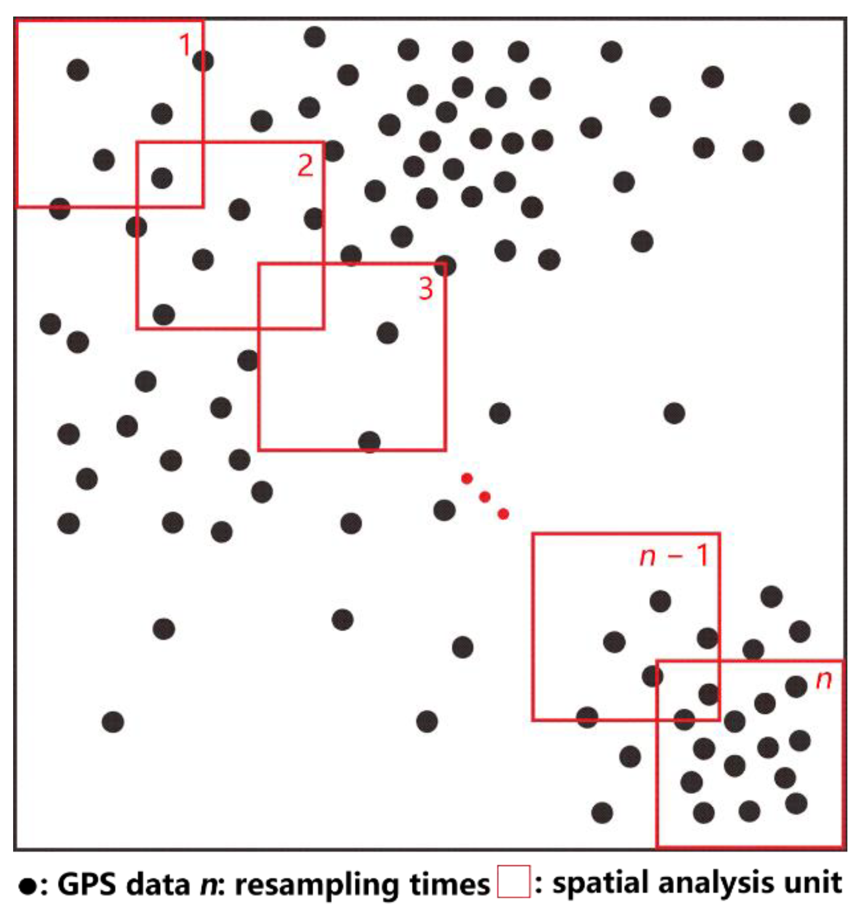
Sensitivity analysis is a common method for evaluating the robustness of Pareto optimality, and this approach can be used to calculate the stability of results from Pareto optimal solutions over multiple calculations [34]. In this paper, a position-based resampling method is used to obtain a relatively stable Pareto-optimal solution in multiple runs. That is, the grid position in the study area was moved while keeping the spatial and temporal resolutions unchanged to resample the trajectory data. A robustness analysis of the obtained optimal spatiotemporal analysis unit can be performed to verify the mitigation of MAUP effects.
Figure 3 shows the resampling strategy for the statistical spatial data distribution; that is, for a certain spatial analysis unit scale, the data distribution in different spatial unit regions is counted, and the corresponding optimal analysis unit is calculated. The spatial data here are similar to floating car track points. After multiple iterations of resampling the spatial data distribution, the overall optimal spatial analysis unit distribution probability is obtained to analyze the sensitivity of the results of the optimal spatial analysis unit.
3. Experiment and Results
The effectiveness of the multicriteria-based spatiotemporal unit optimization framework is explored using floating car data from the Fifth Ring Road in Beijing. First, the different spatial and temporal units are divided. Second, the distribution pattern of the data is determined based on global and local correlations. Then, the Pareto-optimal algorithm is applied to determine the best spatiotemporal analysis unit. Finally, a sensitivity analysis of the optimal spatiotemporal analysis unit is performed.
3.1. GPS Data Distributions with Different Spatiotemporal Units
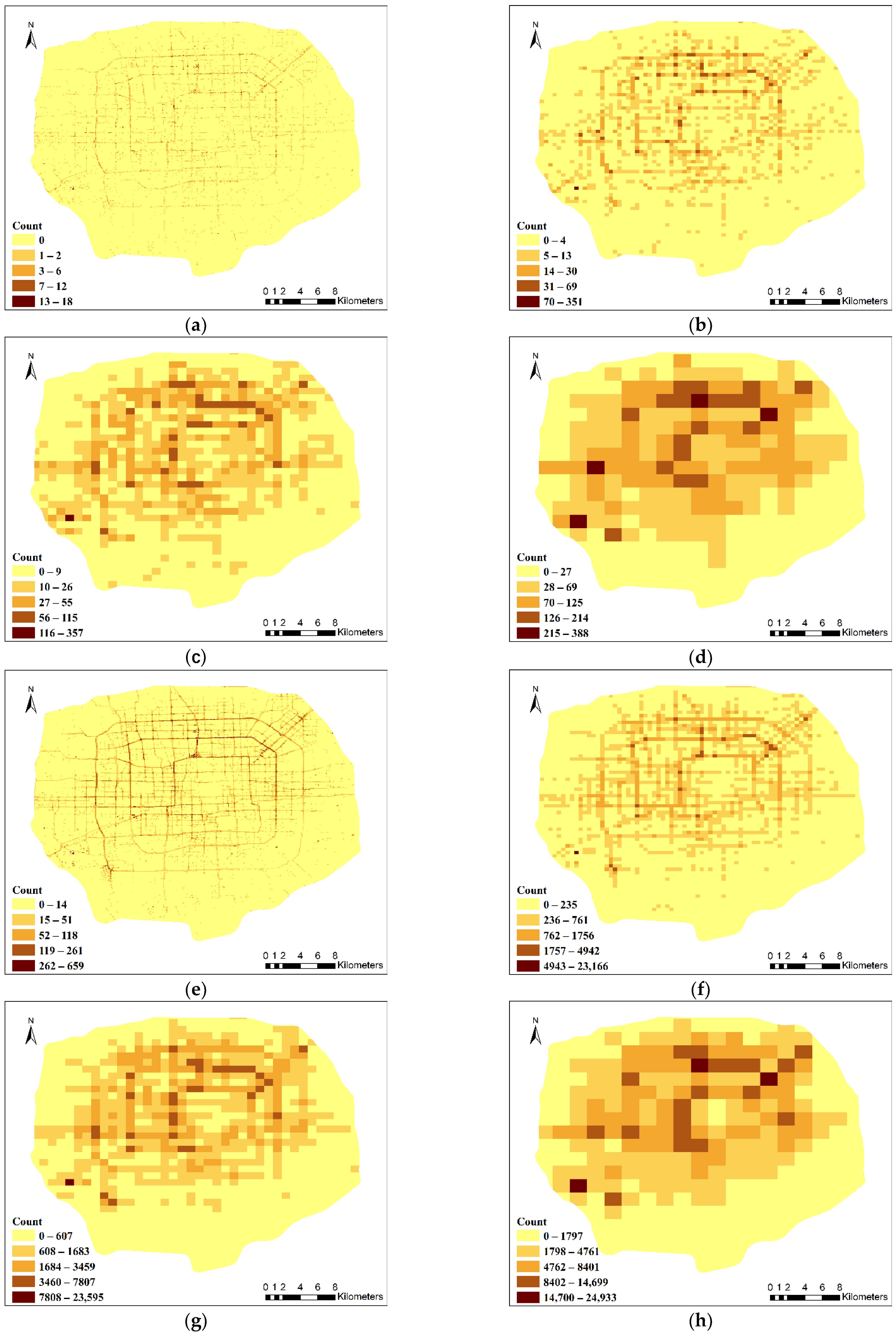
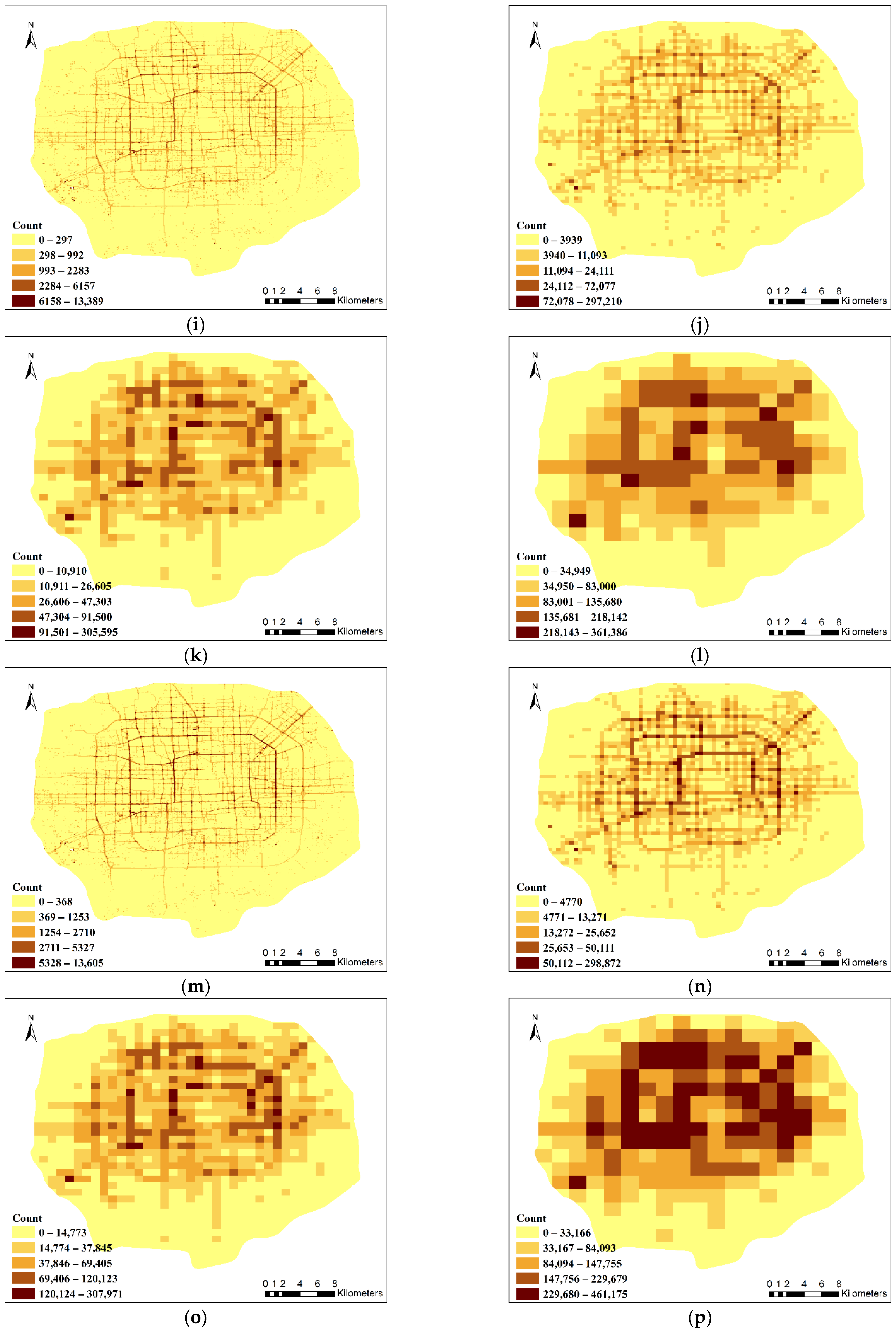
Based on the characteristics of the collected data and practical application cases, the temporal scale of the experiment in this paper is divided into one minute (8:00–8:01), one hour (8:00–9:00), one day (14 November 2012), and two days (14 and 15 November 2012), and the spatial resolution is divided into 100 m, 500 m, 1000 m and 2000 m classes. The distribution of the collected GPS data is determined at four temporal scales and four spatial scales (as shown in Figure 4) for comparison.
The amount of floating car data extracted at the four temporal scales is approximately 15 thousand, 96 thousand, 19 million, and 32 million records. The discrete tracking data are processed at different spatial scales and displayed in grids. At the four spatial scales, the study area is divided into 113,772, 4669, 1209, and 319 grid units. The gridded trajectory frequency not only simplifies the display of discrete point data but also maintains the spatiotemporal and attribute characteristics of the trajectory data. Figure 4 shows the data using the optimal natural breaks method to maximize the differences among the various categories of data. With this method, clustering can be achieved very well, so that the differences between categories are obvious, while the differences within the categories are small, and there is an obvious break between each category. The darker the color in the figure is, the greater the trajectory frequency, and vice versa.
3.2. Global Spatial Correlation and Local Spatial Stability
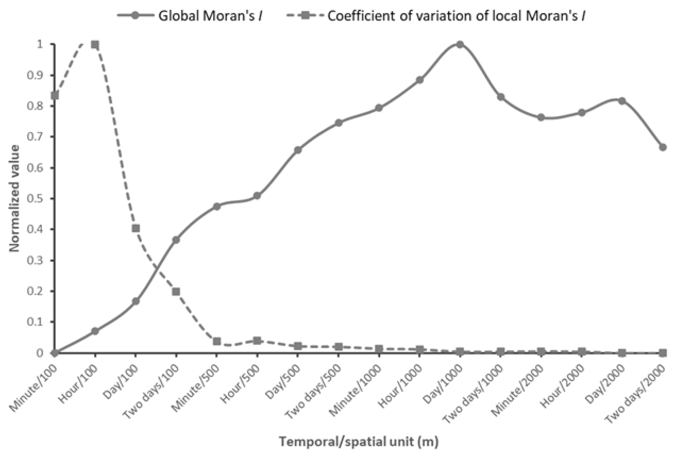
Based on the GPS data at 16 different spatiotemporal scales, the spatiotemporal patterns of the data are calculated using global and local correlations. The 16 spatiotemporal analysis units are compared based on the global Moran’s I and the coefficient of variation of local Moran’s I values. Calculating various indicators based on data with different spatiotemporal units enables us to measure the suitability of units in different applications.
A multicriteria-based spatiotemporal analysis unit optimization framework is applied to Wuhan floating car data to determine the most suitable spatiotemporal analysis unit for urban travel pattern mining. The global Moran’s I and the coefficient of variation of local Moran’s I values for different spatiotemporal analysis units are obtained (Table 2). The results can be conveniently compared and displayed by min-max normalization, as shown in Figure 5.
The comparison of spatiotemporal analysis units in Table 2 and Figure 5 indicates that some analysis units exhibit better spatial correlation characteristics, namely, higher global Moran’s I values and lower coefficients of variation of local Moran’s I values. The global and local correlations show increasing and decreasing trends, respectively, among adjacent spatiotemporal units, such as from hour/100 m to minute/500 m. That is, the global Moran’s I increases, and the coefficient of variation of local Moran’s I decreases. According to their definition, both have been promoted in this spatiotemporal unit interval. Thus, the minute/500 m analysis unit has a higher spatial global correlation and lower spatial heterogeneity than the hour/100 m analysis unit. Therefore, the spatial correlation characteristics of the minute/500 m analysis unit are more consistent, which may lead to more reliable analysis results. The analysis unit shifts from hour/500 m to day/1000 m and from minute/2000 m to day/2000 m, displaying similar phenomena.
Moreover, Table 2 and Figure 5 illustrate that when the spatiotemporal analysis unit is day/1000 m and day/2000 m, the global and local indicators reach the optimal values, respectively. Although the global Moran’s I is highest at day/1000 m, the coefficient of variation of local Moran’s I values is lowest at day/2000 m. Therefore, if the evaluation criteria for the spatiotemporal analysis unit are analyzed separately, different optimal spatiotemporal analysis units should be selected. In terms of the overall spatial correlation of the data, the spatiotemporal unit of day/1000 m is optimal, but in terms of the stability of the local spatial distribution, the spatiotemporal unit of day/2000 m is best. A similar conflict occurs between the spatiotemporal analysis units for minute/500 m and hour/500 m. Therefore, when determining the optimal spatiotemporal analysis unit, there may be conflicts among various schemes with different scales.
3.3. Optimal Spatiotemporal Analysis Unit
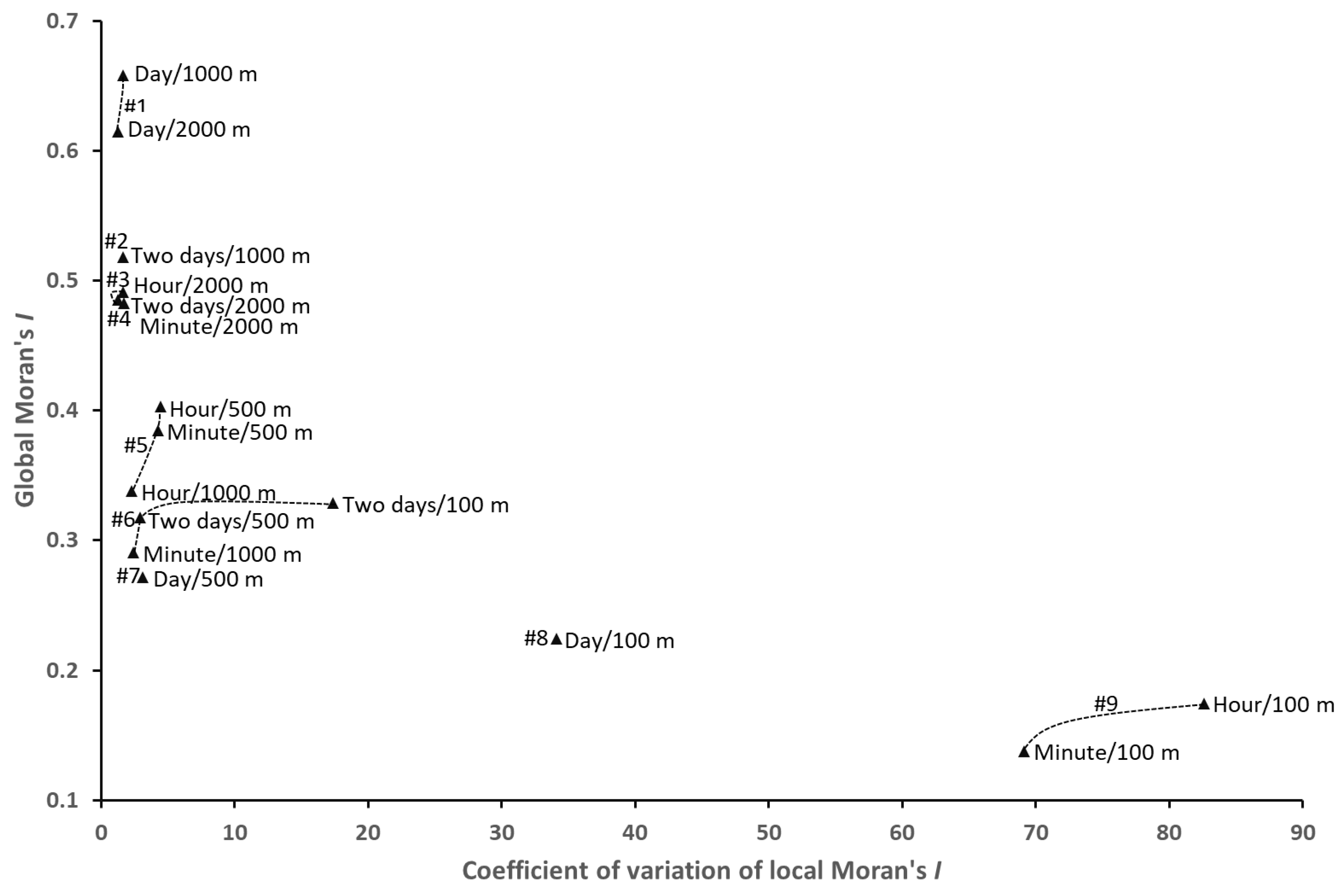
The Pareto-optimal solution is obtained by using the multicriteria optimization framework for spatiotemporal analysis units. According to the global and local spatial correlations, the Pareto boundaries are visualized, and the indicators of the corresponding boundaries (#1–#9) are described (Figure 6 and Table 3). #1 is the first Pareto boundary, which corresponds to the best spatiotemporal analysis unit. From the results, it can be concluded that the optimal spatiotemporal analysis units are day/1000 m and day/2000 m. Day/1000 m has the largest global spatial correlation, while day/2000 m has the least local spatial heterogeneity. Both analysis units are plotted within the first Pareto boundary, and the two solutions can be considered equally good. However, they are dominated by different criteria, with day/1000 m being better than day/2000 m for global Moran’s I and the opposite relation for the coefficient of variation of local Moran’s I. The analysis units within different Pareto boundaries are represented by lines.
In this paper, a position-based resampling method is used to obtain a relatively stable Pareto-optimal solution in multiple runs. Thus, resampling was performed 100 times at each spatiotemporal scale, and the multicriteria optimization framework was run 1600 times to obtain Pareto-optimal analysis units (i.e., the spatiotemporal analysis units within the first Pareto boundary).
As shown in Table 4, the frequencies of day/1000 m and day/2000 m, as optimal spatiotemporal analysis units, are 37.36% and 28.06%, respectively, and they account for 65.42% of the results. Therefore, according to the data used and the study area, the spatiotemporal analysis units of day/1000 m and day/2000 m can be regarded as Pareto-optimal solutions with high robustness. Additionally, the accuracy of the optimization framework for spatiotemporal analysis units based on global and local spatial correlations is verified.
4. Empirical Study
An example involving urban hotspot extraction is used to determine whether the optimal spatiotemporal unit is the optimal scale for geographical phenomenon analysis and to verify the effectiveness of the proposed optimization framework.
4.1. Extraction of Urban Hotspots
The spatial distribution of urban hotspots represents the degree of urbanization [35]. By extracting urban hotspots, we can understand the spatial distribution of a city and the corresponding public issues, and services can be provided to improve daily travel and urban planning. Urban hotspots are usually areas with developed commerce, large flows of people, and established facilities, resulting in dense flows of urban residents [36,37,38]. In a certain area, urban hotspots often have similar function types and distribution scales. The spatial distribution of hotspots is affected by market, transportation, and administrative factors [39]. Therefore, based on residents’ travel data, we can mine urban hot-spots and then perform regional analysis.
Getis and Ord proposed Gi* statistics to measure whether there is local spatial correlation between an observation and its surrounding neighbors [40,41]. Within a given distance range, the attribute sum of an element and its adjacent elements is compared with the attribute sum of all elements, and then, the aggregation degree of attribute values in the local space is described, as shown in Equation (5).
In this equation, n represents the total number of grid units, represents the trajectory frequency in the jth grid, and is the spatial weight of grids i and j. Here, if the distance between the ith and jth grid units is within the given critical distance, they are considered neighbors, and the spatial weight is 1; otherwise, the weight is 0. In this paper, weights are set by determining whether two grids are adjacent. If the two grids are adjacent, the weight is set to 1; otherwise, it is 0. The Getis–Ord Gi* metric can be expressed in normalized form, as shown in Equation (6).
If is positive and the value is large, the frequency of trajectories around grid unit i is relatively large (higher than the average value), and a high-value spatial cluster (hotspot) is present. When the value is negative and small, a low-value spatial cluster (cold spot) is present in grid unit i.
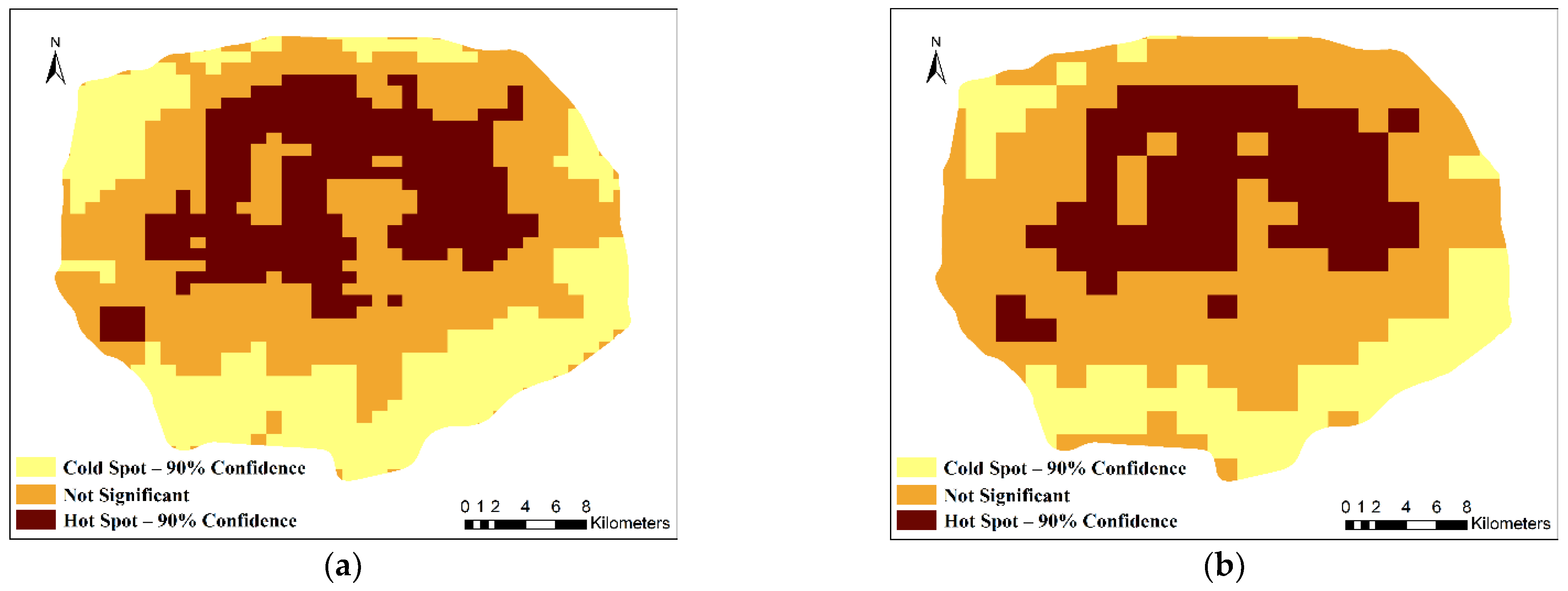
Based on the Getis–Ord Gi* method, the presence of statistically significant high and low values in the trajectory data within the Fifth Ring Road in Beijing is evaluated, and a visual method is used to display the clustered areas. The hotspot distribution based on floating car data in different spatiotemporal units is obtained with the Getis–Ord Gi* method. Representative results are shown in Figure 7.
According to the temporal and spatial distributions of urban hotspots, the proportion of grids with hotspots in the study area can be counted, as shown in Table 5 (90% confidence). Overall, at the same temporal scale, as the spatial analysis scale increases, the proportion of hotspots decreases, and at the same spatial scale, the proportion of hotspots increases as the temporal scale increases. However, within the same spatial unit (1000 m and 2000 m), the proportion of hotspots with day as the temporal unit is slightly higher than that for other temporal units; under the same temporal unit (day), the proportion of hotspots with 1000 m and 2000 m as the spatial units is slightly higher than that for other spatial units. This finding suggests that the highest amount of hotspot distributions is obtained for day/1000 m and day/2000 m. It is optimal to analyze the functional categories of hotspots at these two spatiotemporal units.
4.2. Comparison of the Functions of Urban Hotspots in Different Spatiotemporal Units
Urban hotspots usually have developed commerce, well-established service facilities, and accessible transportation and are areas of concentrated public activities, such as shopping malls, leisure and entertainment facilities, schools, and catering facilities. Therefore, the differences in the distribution of hotspots at different spatiotemporal scales are analyzed from the perspective of the distribution of types of urban spatial functions.
Point of interest (POI) data are closely related to people’s lives and can be used to define the different functional structures of cities. Therefore, POI data can reflect the functional distribution of an urban space. In this paper, POI data are used to calculate the land use types in the study area and then identify the functional distribution of urban hotspot areas. A total of 345,177 POIs with geographic entity location and attribute information were obtained in the study area and divided into 7 functional categories (residence, medical and health, financial, culture and education, office, catering and shopping, and entertainment). The details are shown in Table 6.
According to the distribution of POIs at different scales, FD/CP indicators are used to determine the urban function types for different analysis units [42]; this approach can eliminate the influence of the frequency of different types of POIs on the function identification results. The corresponding equations are shown in (7) and (8).
where i is a POI category, m is the total number of POI categories, is the number of POIs in category i in cluster c, is the total number of POIs in category i, represents the frequency density of the ith category of the POI in cluster c, and represents the proportion of the frequency density of the ith category of the POI in cluster c to the frequency density of all categories of POIs in the cluster.
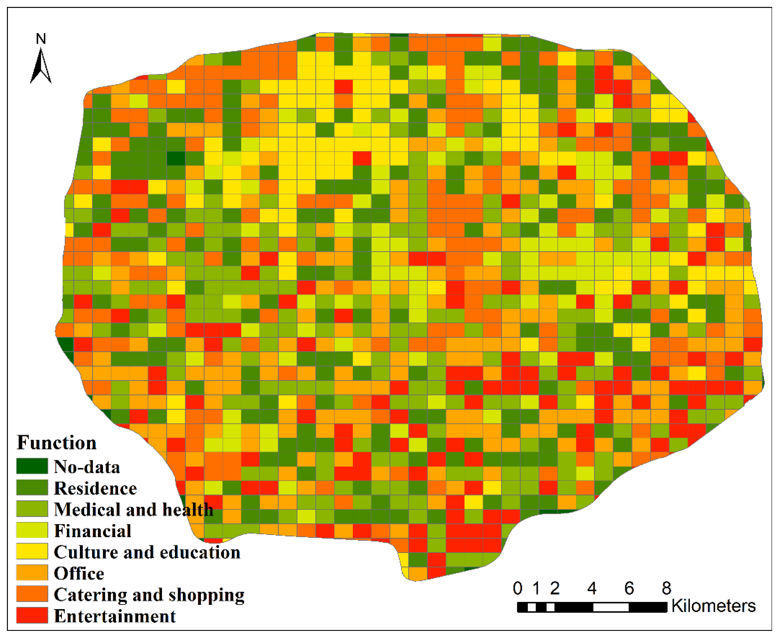
In this paper, the POI category with the largest CP is used as the functional type for the region, and the distribution of the final identified functional types is shown in Figure 8. With this method, the function types can be determined for different hotspot areas with different spatiotemporal units, and the corresponding distribution proportions can be obtained, as shown in Table 7.
The functional category calculated by the POI data corresponds to the hotspot distribution area, and the functional category of the hotspot is obtained. According to the definition of hotspots, the areas that meet the functional characteristics of hotspots can be known. Table 7 shows that the types of hotspot functions at the temporal scale of day and the spatial scales of 1000 m and 2000 m best reflect the actual functions of urban hotspots. At these spatial and temporal scales, catering and entertainment hotspots account for nearly 40% of all hotspots; if office and cultural function types are added, this total increases to more than 70%. Hotspots are usually distributed in densely populated areas. According to the analysis of national demographic data, from the perspective of population distribution, the calculated hotspot areas are consistent with the population distribution pattern of Beijing (the northern part of Beijing’s Fifth Ring Road zone is more populated than the southern part). According to the calculation of the distribution of urban hotspots, it is shown that the spatiotemporal units of day/1000 m and day/2000 m are the optimal spatiotemporal scales, which are consistent with the results calculated by the spatiotemporal analysis unit optimization framework. Therefore, from the distribution of functional types and population distribution in relation to urban hotspots, the accuracy of the optimization framework for spatiotemporal data analysis units is further verified.
4.3. Consistency of Urban Hotspots in Different Spatiotemporal Units
The kappa coefficient is an indicator of the consistency of tests and can be used to measure the effect of classification [43,44]. In classification problems, consistency is used to determine whether the results of a model are consistent with the actual values. That is, the kappa value can measure the degree of consistency between two observed objects. The kappa coefficient is calculated with Equation (9).
where is the sum of the number of correctly classified samples for each class divided by the total number of samples, which is the overall classification accuracy. Assuming that the number of real samples of each class is , the number of predicted samples of each class is , and the total number of samples is n, then . Therefore, the kappa coefficient is calculated based on the confusion matrix of the actual class and the predicted class, and its value falls within the range of [−1, 1]. Usually, the kappa coefficient varies from 0~1, and values in this range can be divided into five groups to indicate different levels of consistency (0.0~0.20 for slight consistency, 0.21~0.40 for fair consistency, 0.41~0.60 for moderate consistency, 0.61~0.80 for substantial consistency, and 0.81~1 for very high consistency).
The kappa coefficient can be used to verify the consistency of hotspots identified at different spatial and temporal scales to illustrate the effects of considering various scales on the data analysis results. Assuming that the distributions of hotspots at scales A and B are compared (here, A and B correspond to certain spatiotemporal scales, respectively, and A and B are different) and that the hotspots obtained at scale B are correct, then represents the sum of the correctly identified hotspot grids in A divided by the total number of grids, and represents the product of the number of correctly identified hotspot grids in A and the total number of hotspot grids divided by the square of the total number of grids.
To analyze the consistency of the hotspot distribution more precisely, this paper uses the overall kappa coefficient proposed by Hagen to compare hotspots at different spatiotemporal scales [45]. The overall kappa coefficient is calculated by the product of the independent indicators Khisto and Klocation. Klocation is an indicator that measures the similarity of two categories based on spatial location. Khisto is a measure of the similarity of two categories based on statistics. Therefore, the overall kappa coefficient can be expressed as a combination of quantitative and positional similarity.
By using the calculation method proposed by Hagen, the overall kappa coefficients at different temporal scales and the same spatial scale (Table 8) and at different spatial scales and the same temporal scale (Table 9) can be obtained. Furthermore, the effects of spatial and temporal scales on the distribution of urban hotspots are studied.
The mean values in Table 8 show that when the spatial scales are the same, the distribution of hotspots at different temporal scales is highly consistent. Thus, in a certain study area, the temporal scale of data analysis has little effect on the study of geographical phenomena.
The mean values in Table 9 indicate that when the temporal scales are the same, the distribution of hotspots at different spatial scales displays low consistency. Notably, in a certain study area, the spatial scale of data analysis, that is, the unit size, has a large impact on the study of geographical phenomena. This result verifies the importance of MAUP effects.
In summary, compared with the temporal scale, the spatial scale has a greater impact on the analysis of geographical phenomena. The larger the temporal unit selected for data analysis, the more data are included, whereas the smaller the temporal unit is, the less data are included. Even if the data volume increases, the data distribution in the study area does not considerably change; that is, the selection of the temporal scale has little effect on the data analysis. However, different spatial scales have a greater impact on the data distribution and influence the calculation results for geographical phenomena. Therefore, when analyzing geographical phenomena, optimization of the spatial analysis unit should be prioritized.
5. Discussion
The traditional spatiotemporal analysis unit is subjectively established according to the analyst’s point of view and application field [46,47,48]. There are often no criteria or reasons to ensure the representativeness of the analytical units, which may give rise to MAUP effects [7,8]. This paper argues that a multicriteria-based data-driven approach can be used to provide analysis units that fit the real world.
Geographical phenomenon analysis is generally affected by both temporal and spatial scales and involves analyzing as many temporal and spatial scales as possible to determine optimal units, and using multiple criteria to automatically evaluate the analysis results. The previous determination methods of analytical units based on a single criterion such as global correlation have uncertainties [49]. Different standards affect the selection of units from different angles and lead to differences in the analysis results. Therefore, we propose a framework based on Pareto optimality methods, which can flexibly select suitable units based on multiple criteria to satisfy arbitrary optimization criteria for different datasets and analysis regions. Furthermore, this paper considers not only the spatial scale but also the temporal scale. Time segmentation and aggregation are means of analyzing real-world spatiotemporal processes, and data aggregation at different temporal scales imposes an impact on the results [50].
In this paper, there may be conflicts when applying a data-driven approach based on multiple criteria, such as global correlation versus local correlation. The optimal spatiotemporal unit that fits one criterion may not conform to the other; so, it is necessary to define the size of the unit and the criteria for judgement according to the research topic and knowledge reserve. In addition, the use of regular grids in this paper to divide the space unit has limitations. Geographic phenomena are irregularly distributed. Different types of area units may be studied in the future. At the same time, the uncertainty of the optimal unit increases with the increase in the number of criteria, and more expertise is required to determine the optimal spatiotemporal unit. The optimal spatiotemporal analysis unit may change due to different research data, times, and cases. In the future, other cases and criteria can be used to evaluate the framework proposed in this paper to obtain broader results.
6. Conclusions
The determination of the spatiotemporal scale is the basis for analyses of geographical phenomena using spatiotemporal data. In this paper, a multicriteria-based spatiotemporal analysis unit optimization framework is proposed to assist in determining the optimal spatiotemporal analysis units in spatiotemporal data analyses. Based on Pareto optimality, the framework can be used to evaluate candidate spatiotemporal analysis units based on any number of criteria, thus overcoming the subjectivity and randomness of traditional methods of establishing analysis units and mitigating MAUP effects to a certain extent.
Floating car data are applied to the multicriteria-based spatiotemporal analysis unit optimization framework, and the optimal spatiotemporal analysis unit is determined by combining the global spatial autocorrelation index and the coefficient of variation of local spatial autocorrelation. The results show that the optimal spatiotemporal analysis units (day/1000 m and day/2000 m) provide a more consistent spatial pattern than other analysis units and may provide more reliable analysis results. The optimal spatiotemporal analysis unit based on multiple criteria also provides a reference analysis scale for studies of urban problems. Moreover, urban hotspot extraction was performed to further illustrate the reliability of the method proposed in this paper. By introducing the proposed method for determining a suitable analysis scale according to the spatial and temporal characteristics of spatiotemporal data, the accuracy of the calculation results for geographical phenomena is improved.
However, due to MAUP effects, the use of different indicators, and differences in application fields, the uncertainty of spatiotemporal analysis units is often an issue. Therefore, when determining the best spatiotemporal analysis unit in studies of geographical phenomena, as many factors as possible, such as other spatial unit shapes and sizes and new evaluation criteria, should be considered.
Author Contributions
Conceptualization, H.C.; methodology, H.C. and L.W.; validation, H.C. and Z.H.; formal analysis, H.C. and L.W.; investigation, H.C.; data curation, H.C.; writing—original draft preparation, H.C.; writing—review and editing, H.C. and L.W.; visualization, H.C. and Z.H.; supervision, L.W.; project administration, L.W.; funding acquisition, L.W. All authors have read and agreed to the published version of the manuscript.
Funding
This study was financially supported by the National Key Research and Development Program (Grant No. 2017YFB0503600).
Data Availability Statement
Taxi GPS data were provided by the Beijing Taxi Operation Company. The POI data were collected from the Baidu map (https://lbsyun.baidu.com/index.php?title=lbscloud/poitags (accessed on 13 July 2021)).
Conflicts of Interest
The authors declare no conflict of interest.
References
- Thrift, N. The Promise of Urban Informatics: Some Speculations. Environ. Plan. A Econ. Space 2014, 46, 1263–1266. [Google Scholar] [CrossRef] [Green Version]
- Yuan, N.J.; Zheng, Y.; Xie, X.; Wang, Y.; Zheng, K.; Xiong, H. Discovering Urban Functional Zones Using Latent Activity Trajectories. IEEE Trans. Knowl. Data Eng. 2015, 27, 712–725. [Google Scholar] [CrossRef]
- Cui, H.; Wu, L.; Hu, S.; Lu, R.; Wang, S. Recognition of Urban Functions and Mixed Use Based on Residents’ Movement and Topic Generation Model: The Case of Wuhan, China. Remote Sens. 2020, 12, 2889. [Google Scholar] [CrossRef]
- Yang, H.; Zhang, X.; Li, Z.; Cui, J. Region-Level Traffic Prediction Based on Temporal Multi-Spatial Dependence Graph Convolutional Network from GPS Data. Remote Sens. 2022, 14, 303. [Google Scholar] [CrossRef]
- Openshaw, S. An Empirical Study of Some Zone-Design Criteria. Environ. Plan. A Econ. Space 1978, 10, 781–794. [Google Scholar] [CrossRef]
- Chen, X.; Nordhaus, W.D. VIIRS Nighttime Lights in the Estimation of Cross-Sectional and Time-Series GDP. Remote Sens. 2019, 11, 1057. [Google Scholar] [CrossRef] [Green Version]
- Jiang, B.; Miao, Y. The Evolution of Natural Cities from the Perspective of Location-Based Social Media. Prof. Geogr. 2015, 67, 295–306. [Google Scholar] [CrossRef] [Green Version]
- Lee, Y.; Kwon, P.; Yu, K.; Park, W. Method for Determining Appropriate Clustering Criteria of Location-Sensing Data. ISPRS Int. J. Geo-Inf. 2016, 5, 151. [Google Scholar] [CrossRef] [Green Version]
- Meng, Y.; Lin, C.; Cui, W.; Yao, J. Scale selection based on Moran’s I for segmentation of high resolution remotely sensed images. In Proceedings of the 2014 IEEE International Geoscience and Remote Sensing Symposium (IGARSS), New York, NY, USA, 13–18 July 2014; pp. 4895–4898. [Google Scholar] [CrossRef]
- Jelinski, D.E.; Wu, J. The modifiable areal unit problem and implications for landscape ecology. Landsc. Ecol. 1996, 11, 129–140. [Google Scholar] [CrossRef]
- Fotheringham, A.S.; Brunsdon, C.; Charlton, M. Quantitative Geography: Perspectives on Spatial Data Analysis; Sage Publications: London, UK, 2000. [Google Scholar]
- Chen, J.; Zhang, Y.; Yu, Y. Effect of MAUP in Spatial Autocorrelation. Acta Geogr. Sin. 2012, 66, 1597–1606. [Google Scholar] [CrossRef]
- Zhang, J.; Atkinson, P.; Goodchild, M.F. Scale in Spatial Information and Analysis; CRC Press: Boca Raton, FL, USA, 2014. [Google Scholar]
- Chou, Y.H. Map Resolution and Spatial Autocorrelation. Geogr. Anal. 1991, 23, 228–246. [Google Scholar] [CrossRef]
- Qi, Y.; Wu, J. Effects of changing spatial resolution on the results of landscape pattern analysis using spatial autocorrelation indices. Landsc. Ecol. 1996, 11, 39–49. [Google Scholar] [CrossRef]
- Griffith, D.A.; Wong, D.W.S.; Whitfield, T. Exploring Relationships Between the Global and Regional Measures of Spatial Autocorrelation. J. Reg. Sci. 2003, 43, 683–710. [Google Scholar] [CrossRef]
- Openshaw, S.; Taylor, P.J. A million or so correlated coefficients: Three experiments on the modifiable areal unit problem. In Statistical Applications in the Spatial Science; Wrigley, N., Ed.; University of Bristol: Bristol, UK, 1979; pp. 127–144. [Google Scholar]
- Fotheringham, A.S.; Wong, D.W.S. The Modifiable Areal Unit Problem in Multivariate Statistical Analysis. Environ. Plan. A Econ. Space 1991, 23, 1025–1044. [Google Scholar] [CrossRef]
- Cliff, A.D.; Ord, J.K. Spatial Processes, Models and Applications. Econ. Geogr. 1983, 59, 322–325. [Google Scholar] [CrossRef]
- Anselin, L. Spatial Econometrics; Springer: Berlin, Germany, 1988. [Google Scholar]
- Lu, F.; Liu, K.; Chen, J. Research on Human Mobility in Big Data Era. J. Geo-Inf. Sci. 2014, 16, 665–672. Available online: http://www.dqxxkx.cn/EN/10.3724/SP.J.1047.2014.00665 (accessed on 9 December 2021).
- Ta, N.; Shen, Y.; Chai, Y. Progress in research from a lifestyle perspective of space-time behavior. Prog. Geogr. 2016, 35, 1279–1287. [Google Scholar] [CrossRef] [Green Version]
- Pei, T.; Li, T.; Zhou, C. Spatiotemporal Point Process: A New Data Model, Analysis Methodology and Viewpoint for Geoscientific Problem. Geo-Inf. Sci. 2013, 15, 793–800. [Google Scholar] [CrossRef]
- Wang, J.; Wu, F.; Guo, J.; Cheng, Y.; Chen, K. Challenges and opportunities of spatio-temporal big data. Sci. Surv. Mapp. 2017, 42, 1–7. [Google Scholar] [CrossRef]
- Zhang, Q.; Shi, Q.; Yao, J. Using multi-criteria decision analysis technology to evaluate technical renovation projects. China Soft Sci. 1997, 2, 70–73. Available online: https://d.wanfangdata.com.cn/periodical/zgrkx199702013 (accessed on 25 November 2021).
- Xu, D.-L. An introduction and survey of the evidential reasoning approach for multiple criteria decision analysis. Ann. Oper. Res. 2012, 195, 163–187. [Google Scholar] [CrossRef]
- Wielgosz, M.; Malyszko, M. Multi-Criteria Selection of Surface Units for SAR Operations at Sea Supported by AIS Data. Remote Sens. 2021, 13, 3151. [Google Scholar] [CrossRef]
- Beijing Transport Institute. Available online: http://www.bjtrc.org.cn/List/index/cid/7.html (accessed on 9 September 2013).
- Beijing Municipal Bureau of Statistics. Available online: http://tjj.beijing.gov.cn/tjsj_31433/ (accessed on 1 March 2022).
- de Andrade, S.C.; Restrepo-Estrada, C.; Nunes, L.H.; Rodriguez, C.A.M.; Estrella, J.C.; Delbem, A.C.B.; de Albuquerque, J.P. A multicriteria optimization framework for the definition of the spatial granularity of urban social media analytics. Int. J. Geogr. Inf. Sci. 2021, 35, 43–62. [Google Scholar] [CrossRef]
- Luo, L.; Wei, H. Statistics; Chinese financial & Economic Publishing House: Beijing, China, 2011. [Google Scholar]
- Li, S.; Li, H. Interpretation of Management Terminology; Enterprise Management Publishing House: Beijing, China, 2007. [Google Scholar]
- Adayel, R.; Bazi, Y.; Alhichri, H.; Alajlan, N. Deep Open-Set Domain Adaptation for Cross-Scene Classification based on Adversarial Learning and Pareto Ranking. Remote Sens. 2020, 12, 1716. [Google Scholar] [CrossRef]
- Fonseca, V.G.D.; Fonseca, C.M.; Hall, A.O. Inferential performance assessment of stochastic optimisers and the attainment function. In Proceedings of the First International Conference on Evolutionary Multicriterion Optimization, Berlin, Germany, 7–9 March 2001; pp. 213–225. [Google Scholar] [CrossRef]
- Zhang, Q.; Seto, K.C. Mapping urbanization dynamics at regional and global scales using multi-temporal DMSP/OLS nighttime light data. Remote Sens. Environ. 2011, 115, 2320–2329. [Google Scholar] [CrossRef]
- Zheng, Y.; Zhang, L.; Xie, X.; Ma, W.Y. Mining interesting locations and travel sequences from GPS trajectories. In Proceedings of the 18th International Conference on World Wide Web, Madrid, Spain, 20–24 April 2009; pp. 791–800. [Google Scholar] [CrossRef] [Green Version]
- Chang, H.W.; Tai, Y.C.; Hsu, J.Y.J. Context-aware taxi demand hotspots prediction. Int. J. Bus. Intell. Data Min. 2010, 5, 3–18. [Google Scholar] [CrossRef]
- Duan, X.; Hu, Q.; Zhao, P.; Wang, S.; Ai, M. An Approach of Identifying and Extracting Urban Commercial Areas Using the Nighttime Lights Satellite Imagery. Remote Sens. 2020, 12, 1029. [Google Scholar] [CrossRef] [Green Version]
- Friedmann, J. Four Theses in the Study of China’s Urbanization. Int. J. Urban Reg. Res. 2006, 30, 440–451. [Google Scholar] [CrossRef]
- Getis, A.; Ord, J.K. The Analysis of Spatial Association by Use of Distance Statistics. Geogr. Anal. 1992, 24, 189–206. [Google Scholar] [CrossRef]
- Ord, J.K.; Getis, A. Local Spatial Autocorrelation Statistics: Distributional Issues and an Application. Geogr. Anal. 1995, 27, 286–306. [Google Scholar] [CrossRef]
- Yu, L.; He, X.; Liu, J. Discovering urban functional regions based on sematic mining from spatiotemporal data. J. Sichuan Univ. 2019, 56, 246–252. [Google Scholar] [CrossRef]
- Kitada, K.; Fukuyama, K. Land-Use and Land-Cover Mapping Using a Gradable Classification Method. Remote Sens. 2012, 4, 1544–1558. [Google Scholar] [CrossRef] [Green Version]
- Tang, W.; Hu, J.; Zhang, H.; Wu, P.; He, H. Kappa coefficient: A popular measure of rater agreement. Shanghai Arch. Psychiatry 2015, 27, 62–67. Available online: https://d.wanfangdata.com.cn/periodical/shjsyx201501011 (accessed on 15 October 2021). [PubMed]
- Hagen, A. Multi-method assessment of map similarity. In Proceedings of the 5th AGILE Conference on Geographic Information Science, Palma, Spain, 25–27 April 2002; pp. 1–8. Available online: https://www.researchgate.net/publication/228862291_Multi-method_assessment_of_map_similarity (accessed on 25 February 2022).
- Openshaw, S.; Rao, L. Algorithms for Reengineering 1991 Census Geography. Environ. Plan. A 1995, 27, 425–446. [Google Scholar] [CrossRef]
- Jiang, B.; Brandt, S.A. A Fractal Perspective on Scale in Geography. ISPRS Int. J. Geo-Inf. 2016, 5, 95. [Google Scholar] [CrossRef] [Green Version]
- Poorthuis, A. How to Draw a Neighborhood? The Potential of Big Data, Regionalization, and Community Detection for Understanding the Heterogeneous Nature of Urban Neighborhoods. Geogr. Anal. 2018, 50, 182–203. [Google Scholar] [CrossRef]
- Openshaw, S. A Geographical Solution to Scale and Aggregation Problems in Region-Building, Partitioning and Spatial Modelling. Trans. Inst. Br. Geogr. 1977, 2, 459–472. [Google Scholar] [CrossRef]
- Cheng, T.; Adepeju, M. Modifiable Temporal Unit Problem (MTUP) and Its Effect on Space-Time Cluster Detection. PLoS ONE 2014, 9, e100465. [Google Scholar] [CrossRef] [Green Version]
Figure 1.
Overall workflow.

Figure 2.
Study area: Fifth Ring Road area of Beijing.

Figure 3.
Resampling method based on spatial location (1, 2, ... n represent the sampling times).

Figure 4.
GPS data distributions based on different spatial and temporal units: (a) minute/100 m; (b) minute/500 m; (c) minute/1000 m; (d) minute/2000 m; (e) hour/100 m; (f) hour/500 m; (g) hour/1000 m; (h) hour/2000 m; (i) day/100 m; (j) day/500 m; (k) day/1000 m; (l) day/2000 m; (m) two days/100 m; (n) two days/500 m; (o) two days/1000 m; and (p) two days/2000 m.


Figure 5.
Normalized global spatial correlation and local spatial stability.

Figure 6.
Pareto boundaries based on global and local spatial correlations (#1–#9 are Pareto boundaries).
Figure 6.
Pareto boundaries based on global and local spatial correlations (#1–#9 are Pareto boundaries).

Figure 7.
Distributions of urban hotspots for two significant spatiotemporal units: (a) day/1000 m and (b) day/2000 m.
Figure 7.
Distributions of urban hotspots for two significant spatiotemporal units: (a) day/1000 m and (b) day/2000 m.

Figure 8.
Distributions of the types of urban functions.


Table 1.
GPS data information.
| ID | Time | Latitude | Longitude | Speed (km/h) | Direction | No-Load Identification |
|---|---|---|---|---|---|---|
| 174853 | 20121101001447 | 116.4548645 | 39.9519463 | 51 | 328 | 1 |
| 453468 | 20121102155618 | 116.2787857 | 39.9250107 | 25 | 180 | 0 |
Table 2.
Global spatial correlation and local spatial stability.
| Spatiotemporal Unit (m) | Global Moran’s I | Coefficient of Variation of Local Moran’s I |
|---|---|---|
| Minute/100 | 0.14 | 69.13 |
| Hour/100 | 0.17 | 82.60 |
| Day/100 | 0.22 | 34.10 |
| Two days/100 | 0.33 | 17.37 |
| Minute/500 | 0.39 | 4.27 |
| Hour/500 | 0.40 | 4.47 |
| Day/500 | 0.27 | 3.13 |
| Two days/500 | 0.32 | 2.97 |
| Minute/1000 | 0.29 | 2.45 |
| Hour/1000 | 0.34 | 2.28 |
| Day/1000 | 0.66 | 1.65 |
| Two days/1000 | 0.52 | 1.67 |
| Minute/2000 | 0.48 | 1.75 |
| Hour/2000 | 0.49 | 1.67 |
| Day/2000 | 0.61 | 1.26 |
| Two days/2000 | 0.48 | 1.29 |
Table 3.
Global and local spatial correlations and corresponding Pareto boundaries for each spatiotemporal analysis unit.
Table 3.
Global and local spatial correlations and corresponding Pareto boundaries for each spatiotemporal analysis unit.
| Pareto Boundary | Temporal Unit | Spatial Unit (m) | Global Moran’s I | Coefficient of Variation of Local Moran’s I |
|---|---|---|---|---|
| #1 | Day | 1000 | 0.66 | 1.65 |
| #1 | Day | 2000 | 0.61 | 1.26 |
| #2 | Two days | 1000 | 0.52 | 1.67 |
| #3 | Hour | 2000 | 0.49 | 1.67 |
| #3 | Two days | 2000 | 0.48 | 1.29 |
| #4 | Minute | 2000 | 0.48 | 1.75 |
| #5 | Hour | 500 | 0.40 | 4.47 |
| #5 | Minute | 500 | 0.39 | 4.27 |
| #5 | Hour | 1000 | 0.34 | 2.28 |
| #6 | Two days | 100 | 0.33 | 17.37 |
| #6 | Two days | 500 | 0.32 | 2.97 |
| #6 | Minute | 1000 | 0.29 | 2.45 |
| #7 | Day | 500 | 0.27 | 3.13 |
| #8 | Day | 100 | 0.22 | 34.10 |
| #9 | Hour | 100 | 0.17 | 82.60 |
| #9 | Minute | 100 | 0.14 | 69.13 |
Table 4.
Distribution of optimal spatiotemporal analysis units based on resampling1600 times.
| Temporal Unit | Spatial Unit (m) | Frequency | Frequency Percentage (%) |
|---|---|---|---|
| Day | 1000 | 687 | 37.36 |
| Day | 2000 | 516 | 28.06 |
| Two days | 1000 | 193 | 10.49 |
| Hour | 2000 | 94 | 5.11 |
| Two days | 2000 | 87 | 4.73 |
| Minute | 2000 | 66 | 3.59 |
| Hour | 500 | 51 | 2.77 |
| Minute | 500 | 49 | 2.66 |
| Hour | 1000 | 42 | 2.28 |
| Two days | 100 | 25 | 1.36 |
| Two days | 500 | 18 | 0.98 |
| Minute | 1000 | 11 | 0.60 |
Note: The sum of frequencies is greater than 1600 because the Pareto-optimal boundary may contain one or more spatiotemporal analysis units.
Table 5.
Proportion of hotspots for different spatiotemporal units.
| Temporal Unit | Spatial Unit (m) | Number of Grids with Hotspots | Proportion of Grids with Hotspots |
|---|---|---|---|
| Minute | 100 | 34,328 | 0.30 |
| Minute | 500 | 1023 | 0.22 |
| Minute | 1000 | 222 | 0.18 |
| Minute | 2000 | 64 | 0.20 |
| Hour | 100 | 36,886 | 0.32 |
| Hour | 500 | 1166 | 0.25 |
| Hour | 1000 | 258 | 0.21 |
| Hour | 2000 | 69 | 0.22 |
| Day | 100 | 42,816 | 0.38 |
| Day | 500 | 1401 | 0.30 |
| Day | 1000 | 310 | 0.26 |
| Day | 2000 | 76 | 0.24 |
| Two days | 100 | 42,870 | 0.38 |
| Two days | 500 | 1451 | 0.31 |
| Two days | 1000 | 297 | 0.25 |
| Two days | 2000 | 73 | 0.23 |
Table 6.
POI categories.
| ID | Category Name | Quantity |
|---|---|---|
| 1 | Residence (real estate communities, guesthouses, and hotels) | 17,962 |
| 2 | Medical and health (medical institutions and social security institutions)) | 11,280 |
| 3 | Financial (finance and insurance facilities) | 15,532 |
| 4 | Culture and education (colleges and cultural media) | 30,901 |
| 5 | Office (government agencies and companies) | 30,346 |
| 6 | Catering (restaurants and casual dining) and shopping (shopping malls) | 225,414 |
| 7 | Entertainment (leisure and sports (sports venues and scenic spots)) | 13,742 |
Table 7.
Proportions of functional types in hotspot areas with different spatiotemporal units.
| Spatiotemporal Unit (m)/Function | Residence | Medical and Health | Financial | Culture and Education | Office | Catering and Shopping | Entertainment |
|---|---|---|---|---|---|---|---|
| Minute/100 | 0.12 | 0.20 | 0.19 | 0.15 | 0.14 | 0.06 | 0.14 |
| Minute/500 | 0.13 | 0.18 | 0.13 | 0.14 | 0.15 | 0.13 | 0.14 |
| Minute/1000 | 0.14 | 0.19 | 0.15 | 0.17 | 0.18 | 0.06 | 0.11 |
| Minute/2000 | 0.12 | 0.06 | 0.14 | 0.18 | 0.20 | 0.17 | 0.13 |
| Hour/100 | 0.13 | 0.19 | 0.17 | 0.16 | 0.17 | 0.05 | 0.13 |
| Hour/500 | 0.13 | 0.15 | 0.16 | 0.14 | 0.14 | 0.15 | 0.13 |
| Hour/1000 | 0.12 | 0.18 | 0.16 | 0.17 | 0.13 | 0.11 | 0.13 |
| Hour/2000 | 0.12 | 0.10 | 0.10 | 0.17 | 0.18 | 0.17 | 0.16 |
| Day/100 | 0.13 | 0.20 | 0.18 | 0.15 | 0.15 | 0.07 | 0.12 |
| Day/500 | 0.13 | 0.20 | 0.17 | 0.15 | 0.17 | 0.07 | 0.11 |
| Day/1000 | 0.12 | 0.06 | 0.10 | 0.16 | 0.18 | 0.19 | 0.19 |
| Day/2000 | 0.11 | 0.08 | 0.09 | 0.17 | 0.18 | 0.18 | 0.19 |
| Two days/100 | 0.13 | 0.17 | 0.16 | 0.15 | 0.14 | 0.12 | 0.13 |
| Two days/500 | 0.13 | 0.19 | 0.17 | 0.16 | 0.17 | 0.06 | 0.12 |
| Two days/1000 | 0.10 | 0.07 | 0.13 | 0.16 | 0.19 | 0.20 | 0.15 |
| Two days/2000 | 0.10 | 0.12 | 0.11 | 0.16 | 0.18 | 0.15 | 0.18 |
Table 8.
Overall Kappa coefficients for results based on the same spatial scale and different temporal scales.
Table 8.
Overall Kappa coefficients for results based on the same spatial scale and different temporal scales.
| (m) | Minute/Hour | Minute/Day | Minute/Two Days | Hour/Day | Hour/Two Days | Day/Two Days | Mean |
|---|---|---|---|---|---|---|---|
| 100 | 0.675 | 0.233 | 0.268 | 0.325 | 0.304 | 0.819 | 0.437 |
| 500 | 0.603 | 0.267 | 0.244 | 0.334 | 0.304 | 0.783 | 0.422 |
| 1000 | 0.646 | 0.580 | 0.562 | 0.673 | 0.656 | 0.861 | 0.663 |
| 2000 | 0.660 | 0.429 | 0.397 | 0.410 | 0.413 | 0.852 | 0.527 |
Table 9.
Overall Kappa coefficients for results based on the same temporal scale and different spatial scales.
Table 9.
Overall Kappa coefficients for results based on the same temporal scale and different spatial scales.
| (m) | 100/500 | 100/1000 | 100/2000 | 500/1000 | 500/2000 | 1000/2000 | Mean |
|---|---|---|---|---|---|---|---|
| Minute | 0.249 | 0.190 | 0.144 | 0.388 | 0.318 | 0.480 | 0.295 |
| Hour | 0.259 | 0.163 | 0.122 | 0.361 | 0.241 | 0.442 | 0.265 |
| Day | 0.529 | 0.229 | 0.176 | 0.348 | 0.245 | 0.417 | 0.324 |
| Two days | 0.488 | 0.196 | 0.150 | 0.334 | 0.237 | 0.434 | 0.306 |
Publisher’s Note: MDPI stays neutral with regard to jurisdictional claims in published maps and institutional affiliations. |
© 2022 by the authors. Licensee MDPI, Basel, Switzerland. This article is an open access article distributed under the terms and conditions of the Creative Commons Attribution (CC BY) license (https://creativecommons.org/licenses/by/4.0/).
Share and Cite
MDPI and ACS Style
Cui, H.; Wu, L.; He, Z. Optimization Framework for Spatiotemporal Analysis Units Based on Floating Car Data. Remote Sens. 2022, 14, 2376. https://0-doi-org.brum.beds.ac.uk/10.3390/rs14102376
AMA Style
Cui H, Wu L, He Z. Optimization Framework for Spatiotemporal Analysis Units Based on Floating Car Data. Remote Sensing. 2022; 14(10):2376. https://0-doi-org.brum.beds.ac.uk/10.3390/rs14102376
Chicago/Turabian StyleCui, Haifu, Liang Wu, and Zhenming He. 2022. "Optimization Framework for Spatiotemporal Analysis Units Based on Floating Car Data" Remote Sensing 14, no. 10: 2376. https://0-doi-org.brum.beds.ac.uk/10.3390/rs14102376
Note that from the first issue of 2016, this journal uses article numbers instead of page numbers. See further details here.