
Research on Automatic Identification Method of Terraces on the Loess Plateau Based on Deep Transfer Learning


1
School of Earth Sciences and Engineering, Hohai University, Nanjing 211100, China
2
School of Electronic Engineering and Computer Science, Queen Mary University of London, London E1 4NS, UK
3
Research Center for Eco-Environmental Sciences, Chinese Academy of Sciences, Beijing 210042, China
*
Author to whom correspondence should be addressed.
Remote Sens. 2022, 14(10), 2446; https://0-doi-org.brum.beds.ac.uk/10.3390/rs14102446
Submission received: 4 April 2022
/
Revised: 13 May 2022
/
Accepted: 16 May 2022
/
Published: 19 May 2022
Abstract
:Rapid, accurate extraction of terraces from high-resolution images is of great significance for promoting the application of remote-sensing information in soil and water conservation planning and monitoring. To solve the problem of how deep learning requires a large number of labeled samples to achieve good accuracy, this article proposes an automatic identification method for terraces that can obtain high precision through small sample datasets. Firstly, a terrace identification source model adapted to multiple data sources is trained based on the WorldView-1 dataset. The model can be migrated to other types of images for terracing extraction as a pre-trained model. Secondly, to solve the small sample problem, a deep transfer learning method for accurate pixel-level extraction of high-resolution remote-sensing image terraces is proposed. Finally, to solve the problem of insufficient boundary information and splicing traces during prediction, a strategy of ignoring edges is proposed, and a prediction model is constructed to further improve the accuracy of terrace identification. In this paper, three regions outside the sample area are randomly selected, and the OA, F1 score, and MIoU averages reach 93.12%, 91.40%, and 89.90%, respectively. The experimental results show that this method, based on deep transfer learning, can accurately extract terraced field surfaces and segment terraced field boundaries.
1. Introduction
In the Loess Plateau region of China, the special features of the natural geography have led to severe soil erosion and a large increase in sediment in the Yellow River. The impacts of erosion and sediment seriously restrict the development of the regional economy and further threaten the lives and property of tens of millions of people in downstream areas. Terraces offer significant water storage, support soil conservation, and enhance yields. A terrace’s unique topographic structure is not only able to effectively prevent hydraulic erosion but also provides sufficient retention of soil moisture for vegetation growth, which has been a fundamental measure employed to control soil erosion on sloping land in the Loess Plateau area [1,2,3,4]. Terraces’ maintenance, acceptance, monitoring, and other related work depend on the accuracy of terrace information. Therefore, efficiently yet precisely extracting terrace information offers significant benefits for soil and water conservation planning and monitoring.
The traditional method of manually counting terrace information is labor-intensive and plagued by many limitations. Problems associated with traditional methods include poor repeatability, inefficiency, and long periodicity [5,6]. The development of high-resolution remote-sensing technology has greatly improved the spectral, temporal, and spatial resolution of remote-sensing images. This new technological approach yields richer and more accurate information on terrace characteristics, facilitating the continuous monitoring of terraces [7,8].
Currently, terrace identification based on high-resolution remote-sensing images relies on three primary methods: visual interpretation [9,10,11], Fourier transform (which is based on textural features) [12,13,14], and object-oriented classification [7,15,16]. Human visual interpretation methods have enjoyed widespread use for some time because they do not require site visits. However, this method relies heavily on the expertise of the interpreters. Moreover, the accuracy of the results is difficult to guarantee, and the extraction of large terraces requires a relatively large time investment. The rapid development of high-resolution remote-sensing satellite sensors has made the automatic extraction of spectral textural features based on terraces possible. For example, Zhao et al. [14] used the Fourier transform algorithm to extract the textural features of terraced fields. They found that the method demonstrated high accuracy in identifying the features of small-area terraces. However, in large-area recognition, the irregular textural information of non-terraced types interfered heavily with the results due to more complex landform types. Additionally, misclassification and omission were serious problems, and the accuracy obtained did not meet the needs of engineering production. In contrast, the object-oriented classification method uses meaningful neighboring objects as the basic unit of analysis to extract terraces. Specifically, instead of extracting terraces based on a single feature, this method accounts for information such as the shape, spectrum, and problems. For instance, Diaz-Varela et al. [15] combined DEM and DSM data with high-resolution remote-sensing images to complete terraced fields’ identification by using a multi-scale object classification method. Compared with single remote-sensing image data, the extraction accuracy was indeed improved after DEM and DSM data were added. Yet, the object-oriented classification method mainly relies on manual setting of the segmentation threshold. Subjective factors play too great a role and there is a lack of quantitative analysis, which greatly impacts the classification accuracy and makes it difficult to meet the recognition requirements of terraced fields in massive high-resolution remote-sensing images.
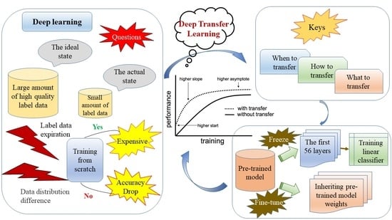
In summary, the described methods for terrace extraction are sensitive to the regional environment but lack the accuracy required to satisfy engineering needs. In contrast, deep learning [17,18] takes an end-to-end approach and pays greater attention to the informational characteristics of the target. This approach can, to an extent, weaken the influence of a complex environment and thus better mine deep information on the research object, to improve the results’ accuracy. The method has been extensively applied in image classification, semantic segmentation, target detection, and other fields [19,20,21,22,23]. Additionally, many scholars have used deep learning methods to extract terraces with high accuracy [24,25]. However, one major problem with deep learning techniques is that they require a large amount of training data to achieve good generalization, making them less effective for minor sample problems. The basic idea of transfer learning is reuse, which refers to taking advantage of similarities between data, tasks, or models to apply knowledge from a secondary domain to a new one, thereby enabling migration and sharing between different tasks [26]. The deep transfer learning [27] method primarily combines deep learning and transfer learning. For small-sample data in complex environments, this method can overcome environmental influences and quickly learn the main features. In addition, the requirements for hardware equipment are low, and the training speed is faster than with the deep learning method. The method has been applied extensively in recent years for target recognition and image classification in the remote-sensing field [28,29,30,31]. Lu et al. [28] proposed a method that combined a deep convolutional neural network and transfer learning (DTCLE) to extract arable land information, achieving an accuracy of up to 90%, which demonstrates the potential of deep transfer learning for information extraction.
To solve the existing problems in the domain of terrace recognition, this investigation proposes a novel method for pixel-level accurate extraction of high-resolution remote-sensing image terraces based on deep transfer learning. The main contributions of this paper are as follows:
- (1)
- A terrace identification source model adapted to multiple data sources is trained based on the WorldView-1 dataset. This model can be migrated to other types of images for terracing extraction as a pre-trained model.
- (2)
- A deep transfer learning method to extract terraces from high-resolution remote-sensing images is proposed. Based on small sample GF-2 datasets, and compared with deep learning and other transfer learning methods, this method can well achieve high-accuracy extraction of small-sample terrace datasets.
- (3)
- Lastly, a prediction model was established to eliminate the border splicing traces and enrich the image edge information. The accuracy evaluation results show that the model can further improve the terrace identification accuracy.
2. Materials and Methods
2.1. Study Area Overview
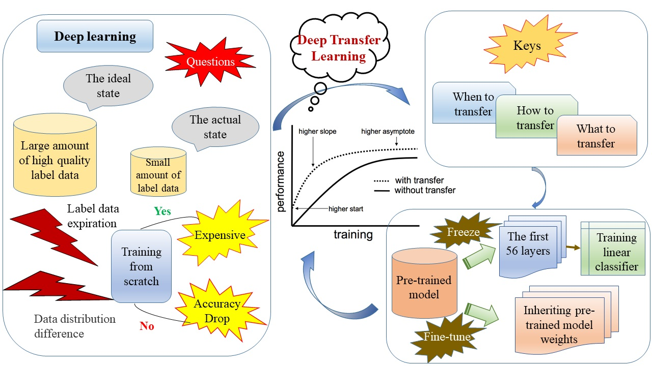
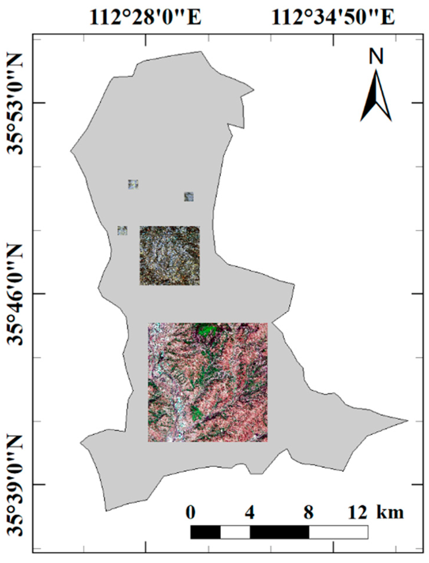
The paper’s study area was located in Duanshi Town, Jincheng City, Qinshui County, Shanxi Province, China, which features a hilly terraced area with extensive loess coverage. The area’s geographical coordinates encompass 35°37′10.12″N to 35°54′19.06″N and 112°25′44.50″E to 112°37′55.07″E. Overlapping mountains, gullies, and ravines, and a wide range of heights, are found within this area, with elevations ranging from 511 to 2358 m. In terms of climate, the annual average temperature falls within the range of 6~12.5 °C, and the annual average precipitation is 560~750 mm. The terraced fields in this region are rich in types and large in area, with obvious traces of human activities and many interferents such as ordinary farmland. It is a complex and representative research area, which can, therefore, well verify the anti-interference ability of a model extracting terraced fields. The geographic location of the study area and the regional remote-sensing images are shown in Figure 1.
2.2. Data Source
Both WorldView-1 and GF-2 satellite remote-sensing image data from Duanshi town in Qinshui County were used as the experimental data in this investigation. These images have also been widely used for image segmentation and target recognition [32,33,34]. The WorldView-1 satellite was launched on September 18, 2007, and its image data comprise only panchromatic images with a spatial resolution of 0.5 m. Meanwhile, the GF-2 satellite was launched on August 19, 2014. It provides panchromatic imagery with a spatial resolution of 0.81 m and multispectral imagery of 3.24 m. The parameters of WorldView-1 and GF-2 satellite images are shown in Table 1 and Table 2, respectively. Other auxiliary data were mainly 2.44-m multispectral image data from the QuickBird satellite, used to fuse WorldView-1 satellite panchromatic images. The smaller the difference in spatial resolution between panchromatic and multispectral images, the better the fusion effect.
2.3. Data Preprocessing
In this investigation, both a WorldView-1 and GF-2 sample area were selected from the research area. The WorldView-1 sample area was 11,000 × 11,000 pixels, demonstrating a wide range, rich terrace types, and sharp features. The GF-2 sample area size was 3400 × 3400 pixels, with a small scope and lower resolution. First, the WorldView-1 panchromatic image was fused with the QuickBird multispectral image using the NNDiffuse Pan Sharpening tool in ENVI 5.3. Then, the GF-2 panchromatic image was fused with the multispectral image by the same method. After fusion, the GF-2 image had four bands, while three bands of RGB were derived. The resolutions of the fused images were 0.5 m2/pixel for WorldView-1 and 0.8 m2/pixel for GF-2.
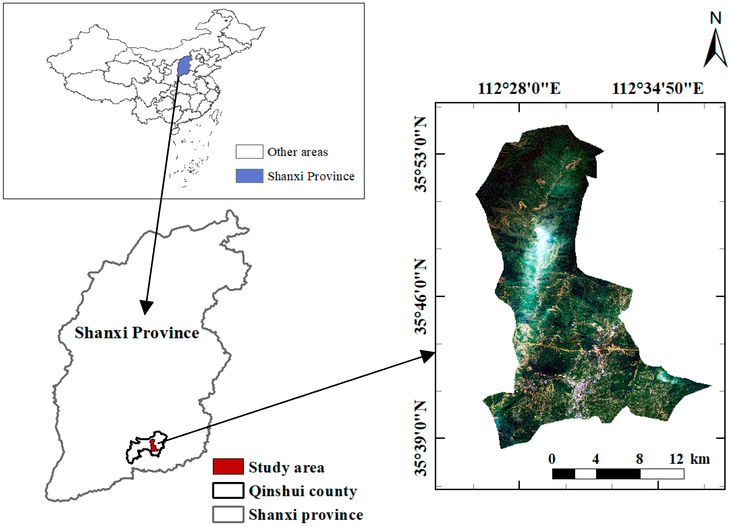
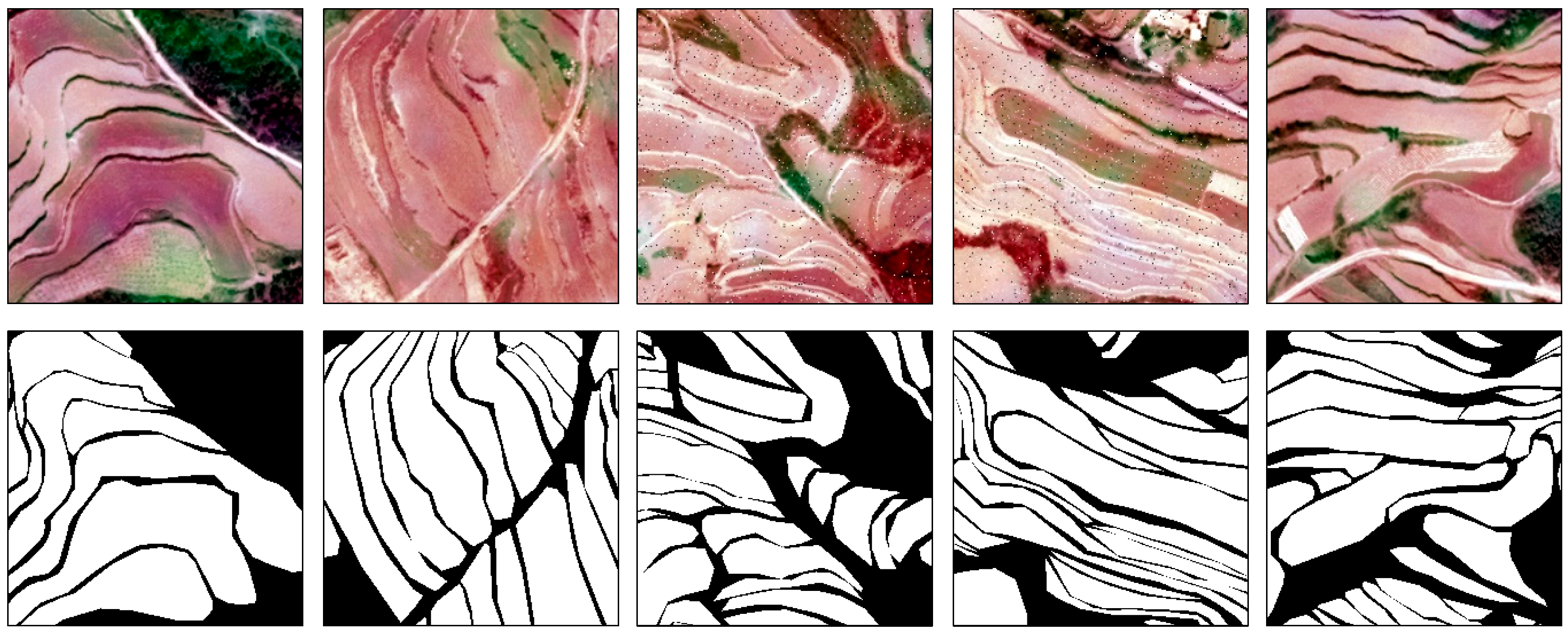
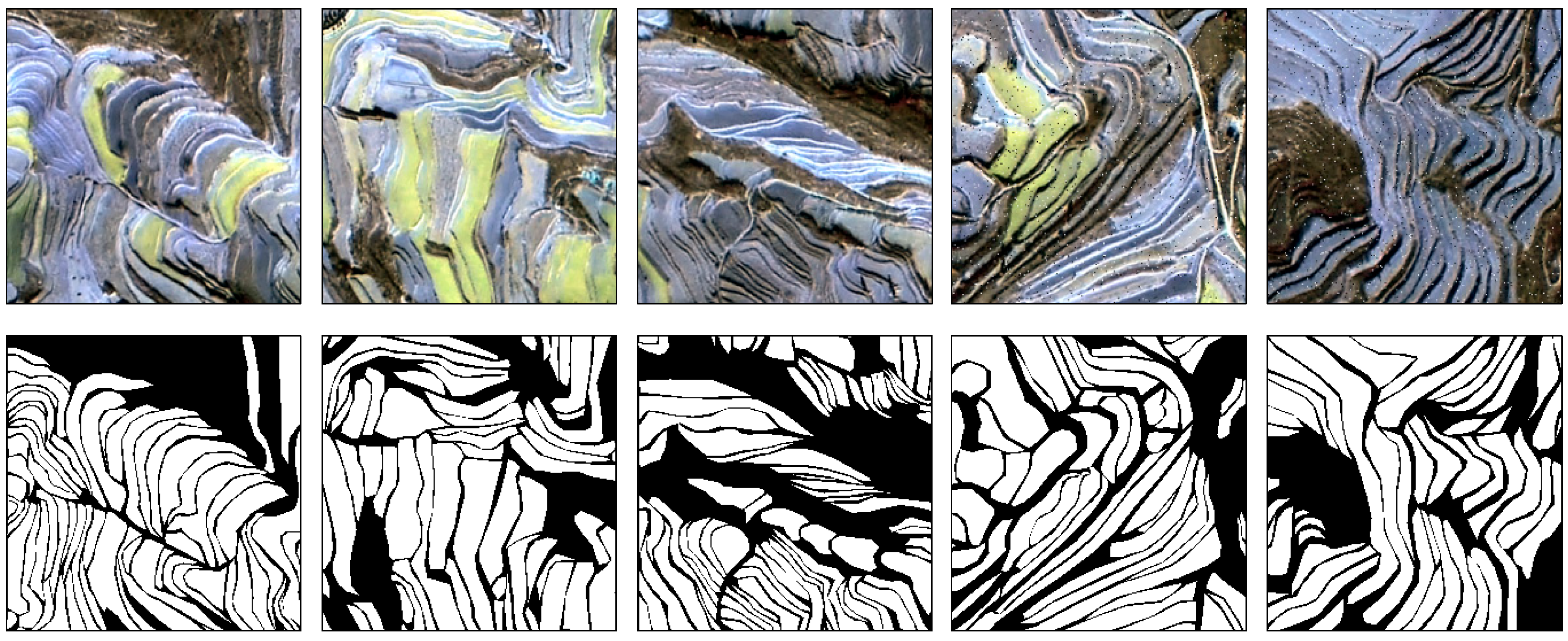
Next, the vector labels of the sample area were created by visual interpretation and manual annotation. The terraced field surface pixel values were set to 255 and labeled using white (RGB (255, 255, 255)). Meanwhile, the other parts’ pixel values were set to 0 and labeled using black (RGB (0, 0, 0)). Then, the Feature to Raster tool of ArcGIS 10.7 was used to complete the production of labels. After the labeling was complete, the processed image and label were cropped with an overlapping sliding window (256 × 256 pixels) and formatted using Python code. A schematic diagram of the overlapping sliding window cropping is shown in Figure 2. Finally, to prevent overfitting, the cropped datasets were augmented by rotating (90°, 180°, 270°), mirroring diagonally, and adding salt and pepper noise. The data were augmented to obtain the WorldView-1 sample dataset of 17,760 sets, including 13,320 sets for training and 4440 sets for validation, and the GF-2 sample dataset of 1300 sets, including 1000 sets for training and 300 sets for validation. The WorldView-1 and GF-2 sample set images are shown in Figure 3 and Figure 4, respectively. The remote-sensing images of the research area were complex, containing roads, buildings, gullies, undeveloped slopes, and a large amount of vegetation. These features other than terraces were called interference elements, which help to verify the ability of the model to correctly extract terrace information.
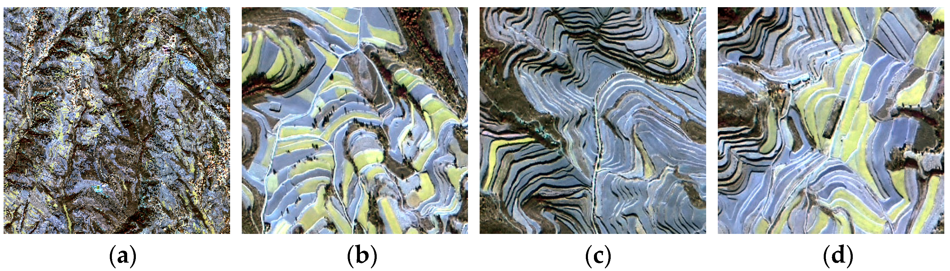
To verify the generalization ability of the proposed method, we selected three representative areas rich in terrace types outside the sample area as the test area from GF-2 images, all 500 × 500 pixels in size. Images of the sample area and each test area are shown in Figure 5. In addition, we show the range and distribution of the WorldView-1 and GF-2 images after fusion, and the geographical relationship of the GF-2 test areas and sample area, in Figure 6.
3. Methods
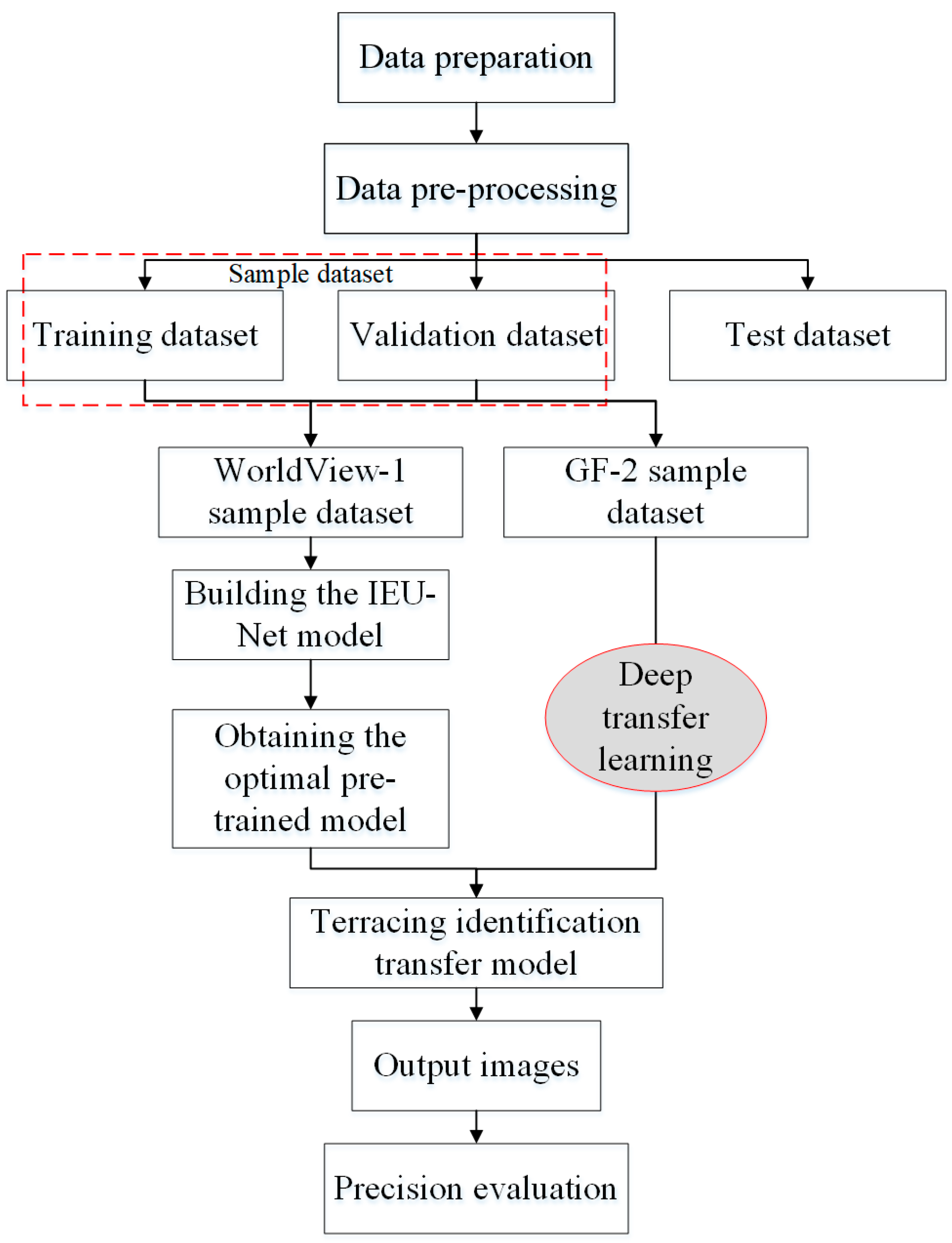
Figure 7 illustrates the flow chart of the method used to accomplish the accurate extraction of terrace surfaces and the accurate segmentation of terrace boundaries. The specific steps are as follows:
- (1)
- Data preprocessing: The images were preprocessed and used as the basis for manual annotation to obtain true sample labels. The sample dataset of 256 × 256 pixels was generated using the sliding window cropping method, and its format was converted from TIFF to PNG. Lastly, data enhancement was performed, and the enhanced data were divided into training and validation datasets.
- (2)
- Building the IEU-Net model: The IEU-Net model was constructed based on the U-Net model for deep feature extraction of high-resolution remote-sensing data.
- (3)
- Obtaining the optimal pre-training model for terrace identification: The WorldView-1 sample set was inputted into the IEU-Net model for training. After adjusting the parameters, the optimal WorldView-1 terrace recognition model was saved.
- (4)
- Migration of pre-trained models to GF-2 high-precision recognition of small-sample terraces: Pre-trained model weights were loaded, and the model structure was adjusted. The transfer learning model was then constructed according to the experimental requirements. Different finetuning strategies were used to train some or retrain all parameters. The GF-2 sample set was inputted into the new model for training, parameter comparison, and tuning, and the transfer learning model was saved.
- (5)
- Predict and output images: A prediction model was constructed by ignoring the edge prediction method, and the test set was inputted into the model for prediction, elimination of the border splicing traces, and enrichment of the image edge information.
- (6)
- Precision evaluation: The prediction labels of each test area were compared with the true labels. The evaluation indexes of Overall Accuracy (OA), F1 score, and mean intersection-over-union (MIoU) were selected for accuracy evaluation.
3.1. IEU-Net Model
The U-Net network is based on an end-to-end fully convolutional neural network, which was originally proposed by Ronneberger et al. [35,36]. In the field of semantic segmentation, this method has proven more effective than other image segmentation methods [37]. The U-Net network is named for its “U” shape. The left half is the compressed path, consisting of two 3 × 3 convolutional layers, a ReLU nonlinear transform, and a 2 × 2 max pooling layer, which form a downsampling module. Its primary role is to perform feature extraction. The right half is the extended path, comprising an upsampled convolutional layer, a copy and crop layer, two 3 × 3 convolutional layers, and the ReLU nonlinear transform, which form an upsampling module. It is mainly used to achieve precise positioning. Both the compressed and extended paths have four sampling modules. The IEU-Net network used the U-Net network as the base architecture. It added a dropout layer [38] with a probability of 0.5 after the fourth set of convolution operations, with another dropout layer added after the fifth set. In other words, the neurons were thrown away with a likelihood of 0.5 in each training iteration, as an effective technique to prevent overfitting. In addition, a batch normalization (BN) [39] layer was added after each convolution to normalize the input data before entering the next layer, which offered an effective way to improve the training speed of the network. The structure and number of parameters of the IEU-Net are shown in Table 3. The mathematical expression of the BN layer is shown in Equation (1):
where represents the normalized result of the first layer; represents standard deviation normalization results; and are learning parameters.
In addition, IEU-Net used IELoss [40] as the loss function, which was improved based on the categorical cross-entropy loss (CELoss), as shown in Equation (2):
where is the ratio of the number of pixels in the selected area to the number of pixels in the whole image; is the total number of sample image pixels; is the total number of categories including the background class; is the tensor of channels consisting of 0 and 1; is the tensor consisting of the layer pixel category probability values obtained by propagating the samples forward. The difference between and is generally calculated by the loss function: the smaller the difference, the closer the parameters are to the optimum and the better the model effect.
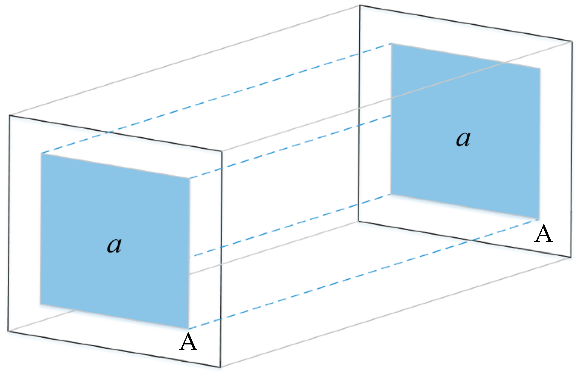
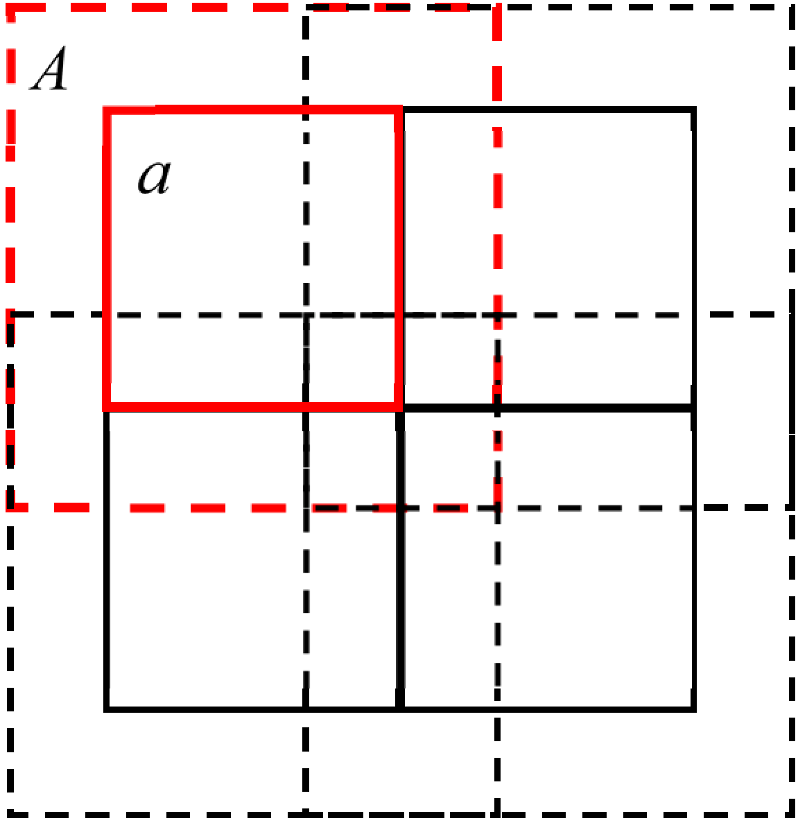
For the IEU-Net model, we selected the middle region for the loss value calculation, instead of the whole image region A. Since the middle region of the image had a wide range of fields, it was easy to determine the category it belonged to by combining its feature information with the surrounding neighborhood information. However, the edge region tended to lose its neighborhood information due to the cropping operation, and the remaining information was not sufficient to determine the category to which it belonged. The general model was trained to reduce the loss value by forcing the edge regions that lacked feature information to fit the truth value. While this approach could lead to overfitting problems due to the lack of image edge information, IELoss could effectively solve this problem and improved the classification accuracy to some extent. Figure 8 presents a schematic diagram of this loss function calculation area.
3.1.1. Feature Mapping Visualization
An essential component of a convolutional neural network is the convolutional layer. It performs most of the computational work in the deep learning process. This layer mainly consists of a superposition of convolutional kernels with a set of fixed weight neurons. Multiple convolutional kernels sliding to carry out convolutional operations in a region will allow the neural network to extract high-level abstract features. The expression of the convolution operation is shown in Equation (3).
where denotes the first row and column pixel values outputted by the feature map after the convolution operation; and denote the width and height of the convolution kernel, respectively; represents the weight parameter of the first row and column of the convolution kernel; is the bias parameter; is the pixel value of row and column of the feature map; is a nonlinear activation function.
Convolutional layers are usually used in combination with activation functions. This technique removes data redundancy by introducing nonlinear factors to simulate the process of biological neurons being stimulated, thus achieving better feature mapping. The commonly used activation functions are sigmoid, TanH, and ReLU, where the ReLU function requires no normalization of the input and has sparse activation compared to the other two functions. Sparse activation [41] means that stimulating neurons to respond selectively to only a few parts of the input signal, and a large number of signals are deliberately blocked. This feature can improve the learning accuracy, extract sparse features better and faster, and prevent overfitting. This investigation used the ReLU activation function, as shown in Equation (4):
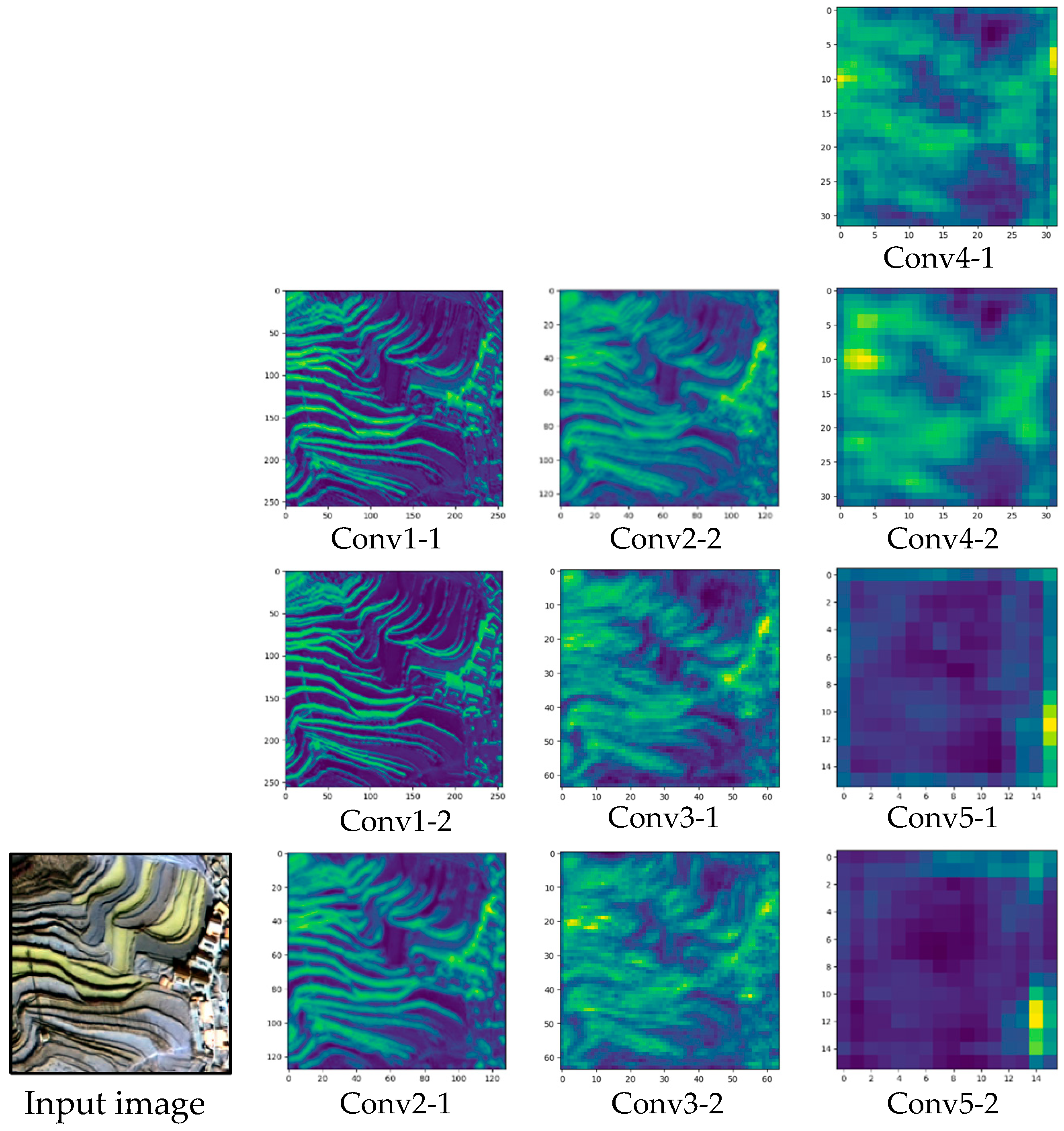
The feature extractor of the IEU-Net in the current model included a total of 10 convolutional layers, all with 3 × 3 convolutional kernels. Figure 9 displays the feature mapping diagram for each layer.
3.1.2. Pooling Operation
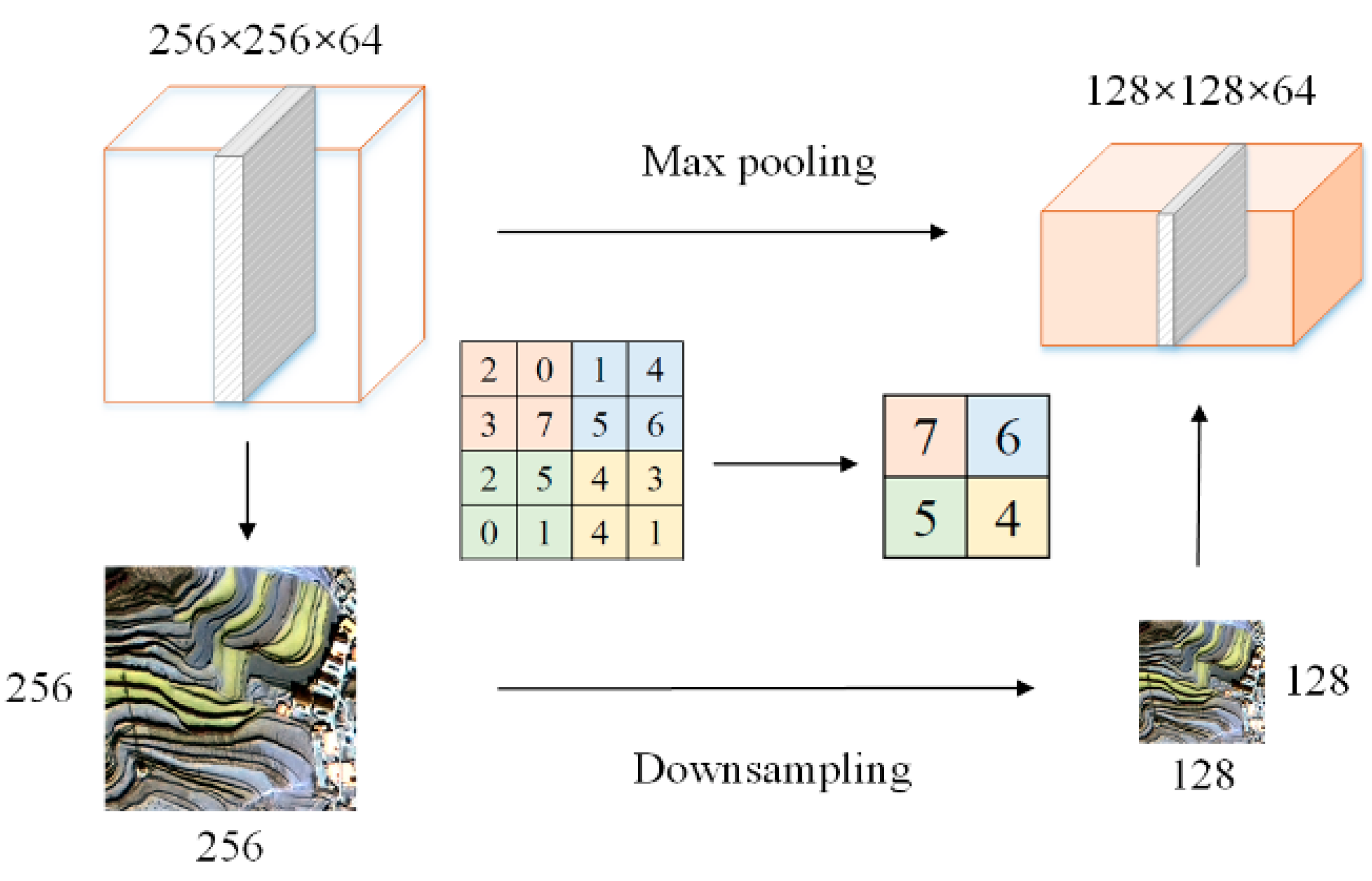
The pooling layer, also known as the downsampling layer, is located between successive convolutional layers, and the basic idea is derived from the visual mechanism. One of its primary functions is to compress the feature map; the compression is in width and height, while the number of channels remains unchanged. The other function is to reduce the number of parameters. In addition, it can reduce the overfitting phenomenon and improve the model’s generalizability. The specific operation of the pooling layer is roughly the same as that of the convolutional layer, except for the operating rules between matrices. It is not affected by backpropagation. Its downsampled convolution kernel generally takes the maximum or average value for the corresponding position, an operation called max pooling or mean pooling, respectively. In this paper, the IEU-Net model adopted the max pooling operation, involving four pooling layers, which were individually located after Conv1-2, Conv2-2, Conv3-2, and Drop4, in order. The pooling kernel was 2 × 2 with a step size of 2. The schematic diagram of the pooling operation is shown in Figure 10.
3.2. Deep Transfer Learning
Transfer learning methods are generally classified as instance-based, feature-based, relationship-based, and model-based transfer learning [42]. This paper focuses on model-based transfer learning: that is, finding common parameters or prior distributions between the spatial models of the source and target data and migrating them. The specific work included both developing and tuning the source model. Since the WorldView-1 terrace data in this case were richer and had a higher resolution, we chose to build a source model adapted to the terrace recognition domain as the learning starting point of the target task. The result was used as a pre-training model to explore the ability of deep transfer learning to accomplish the target task with a small-sample dataset from GF-2.
In this investigation, two finetuning strategies were used for transfer learning, as follows:
- (1)
- Strategy 1: The first 56 layers were used as fixed-invariant feature extractors applied to the new dataset, and a linear classifier was trained based on the new dataset. Since the GF-2 dataset was small, the first 56 layers of the pre-trained model were loaded into the transfer learning model, and its learning rate was set to 0 to freeze the weights and prevent the shallow layers of the model from overfitting the dataset. Essentially, this step fixed the parameters and precluded the weights from being updated during training. The first 56 layers had little to do with specific classification tasks. Therefore, the GF-2 data were used to train only the newly added convolutional layer and the Softmax layer. This method had fewer parameters to train, effectively shortening the training time, but the model training effect was average.
- (2)
- Strategy 2: We loaded all layers of the pre-trained model into the transfer learning model, replaced the classifier in the top layer of the pre-trained model, and retrained it. Next, we initialized the weights of the entire network using the weights of the pre-trained model. The GF-2 dataset was inputted to the transfer learning model, and the weights of the pre-trained network were finetuned by continuing backpropagation with a smaller learning rate based on inherited weights. This method trained identical parameters but saved much time compared to a random initialization network. Moreover, the inherited pre-trained model weights effectively improved the training efficiency, accelerated convergence, improved the model’s generalizability, and obtained good training results.
3.3. Predictive Models
When the model was trained for prediction, inputting the larger remote-sensing images to be classified directly by the network model would have led to a memory overflow. Therefore, the imagery was cropped into a series of smaller images and then those were inputted into the network for prediction. Next, the prediction results were stitched into one final resulting image, following the order of cropping. Since the edge region of each image contained less contextual information, the traditional prediction method of cropping and then stitching with a regular grid would not have been effective, and the prediction results would have been less accurate and shown traces of stitching. To solve this problem, we constructed a prediction model using an edge-ignoring approach. This method first cropped the large image into a series of image blocks, containing specific areas of repetition with neighboring image blocks, and stored them in a chain table. Then, the generator was created, and the prediction procedure was performed. Finally, only the middle part of the prediction result was taken for stitching. The calculation formula for the splicing results is shown in Equation (5):
where represents the prediction results of real clipped images, stands for splicing results, and indicates the overlap ratio, which should match the value of r in IELoss in the IEU-NET model.
A schematic diagram of the prediction method is shown in Figure 11.
4. Experimental Results and Discussion
4.1. Experimental Platform and Parameter Settings
The experimental platform used an Intel Xeon(R) Gold 6130 @ 2.10 GHz 16-core processor, which was configured with 48.0 G RAM (DDR4 2666 MHz) and equipped with an Nvidia GeForce GTX 1080 Ti graphics card with video memory. The experiments were conducted with Anaconda3 (64-bit) as the environment’s configuration. A Windows 10 Professional 64-bit operating system was also used. We created a virtual environment with the conda command and installed Python version 3.6 within the environment. The next step entailed selecting TensorFlow 2.6 as the deep learning framework, using the Keras tool embedded in the framework for model-building. CUDA version 11.2, matching the computer configuration, was selected as the GPU computing platform, and cuDNN 8.1.0 was equipped as the deep learning GPU acceleration library. Finally, PyCharm 2018 was used for deep learning program development and compilation to ensure the smooth running of the experiment.
The Adam optimizer can both adapt to sparse gradients and mitigate gradient oscillations. Additionally, it can adapt to a wide range of models and is computationally efficient. Therefore, this experiment used this optimizer for the loss function. Furthermore, this experiment set the batch size to the power of 2 to bring out the best parallel computing processing power of the GPU with the highest efficiency [43,44,45]. The batch size also accelerated the training of the gradient descent algorithm. After repeated experiments, the optimal pre-training model was found to have parameters that matched the settings for the migration model. Table 4 presents the specific parameters used in the experiment.
4.2. Precision Evaluation Metrics
Accuracy evaluation refers to the contrast of the terrace identification results derived from the experimental method with the actual labels to determine the accuracy of the experimental method. To provide a quantitative description of the effectiveness of GF-2 small-sample terrace identification using transfer learning methods, we used confusion matrices for accuracy evaluation. A confusion matrix is an matrix of the classification results with a statistical classification model. is the class number. The number of categories in this case was 2, and the confusion matrix was 2 × 2; the specific meaning of each field is shown in Table 5.
We chose three evaluation factors: OA, F1 score, and MIoU. OA (Equation (6)) denoted the probability that the classification result predicted by each random sample was consistent with the true type. The F1 score (Equation (7)) was the summed average of the accuracy and recall of the classification model. IOU referred to the ratio of the intersection of the predicted category samples to the actual category samples to the merged set, and MIoU (Equation (8)) expressed the result of summing and averaging the intersection and merging ratios for each category.
where TP is the correctly classified terrace pixel points, FP is the misclassified terrace pixel points, TN is the correctly classified non-terraced pixel points, and FN is the misclassified non-terraced pixel points, while denotes the number of categories.
4.3. Results and Analysis
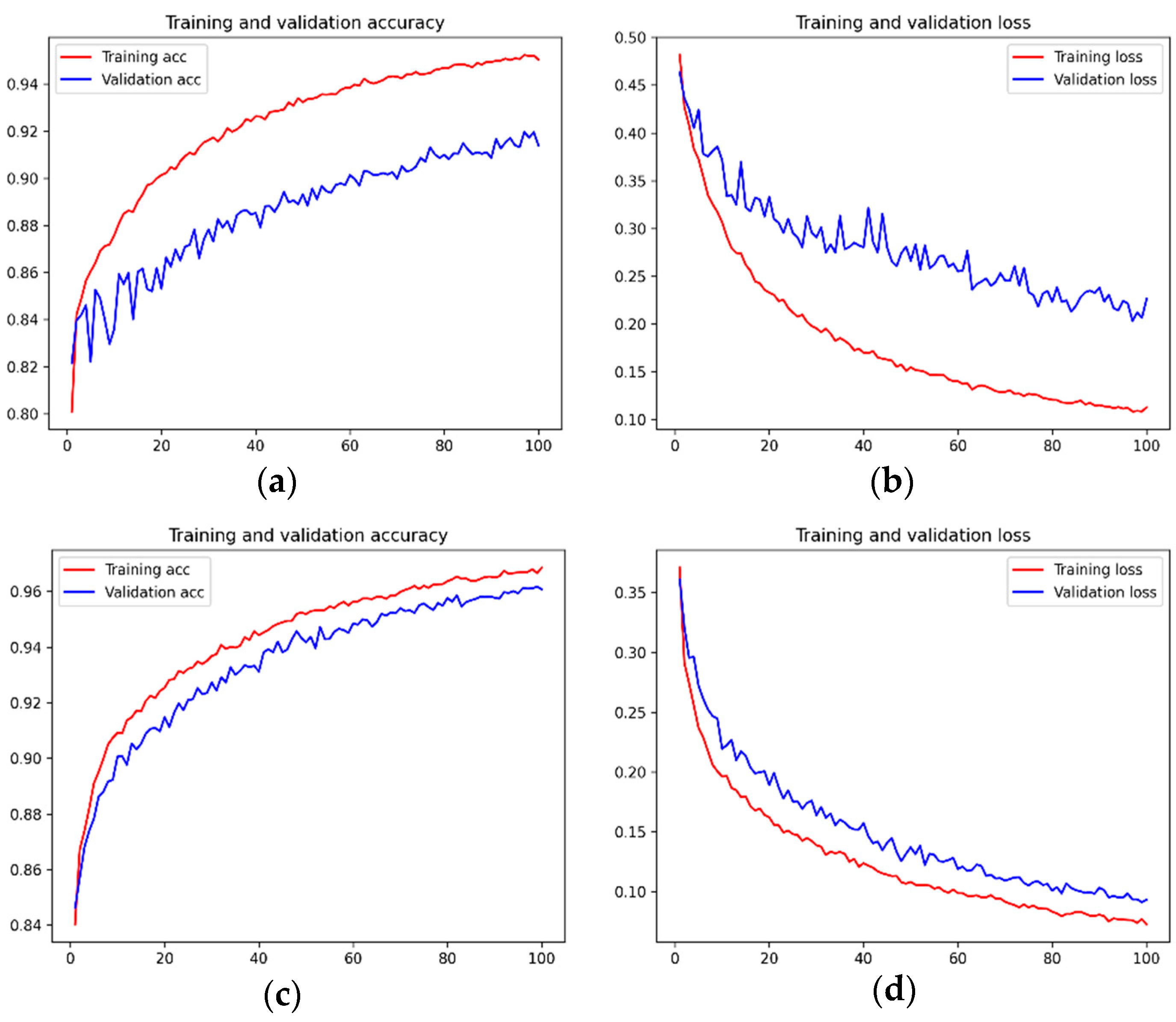
The experiment adopted two finetuning strategies. Since the model trained based on the first strategy was less effective than when using the second strategy, the second strategy was primarily used to migrate the model. The training accuracy of the model and loss graphs are shown in Figure 12. The accuracy of the training and validation datasets of both models in the training process increased slowly with the number of iterations and gradually reached 1. The loss value, meanwhile, slowly decreased until it reached 0. Both steadily leveled off.
After the model was trained, the test set was inputted into the prediction model to carry out predictions. Next, the transfer learning method using the second strategy was compared with both the direct training method and the transfer learning method based on the first strategy. In the direct training method, the weights of the pre-trained model were not inherited, while the IEU-Net model was directly initialized with random weights and trained on the GF-2 small sample dataset. All three methods used the same experimental sample datasets and parameters. The comparison results for the three methods are shown in Figure 13.
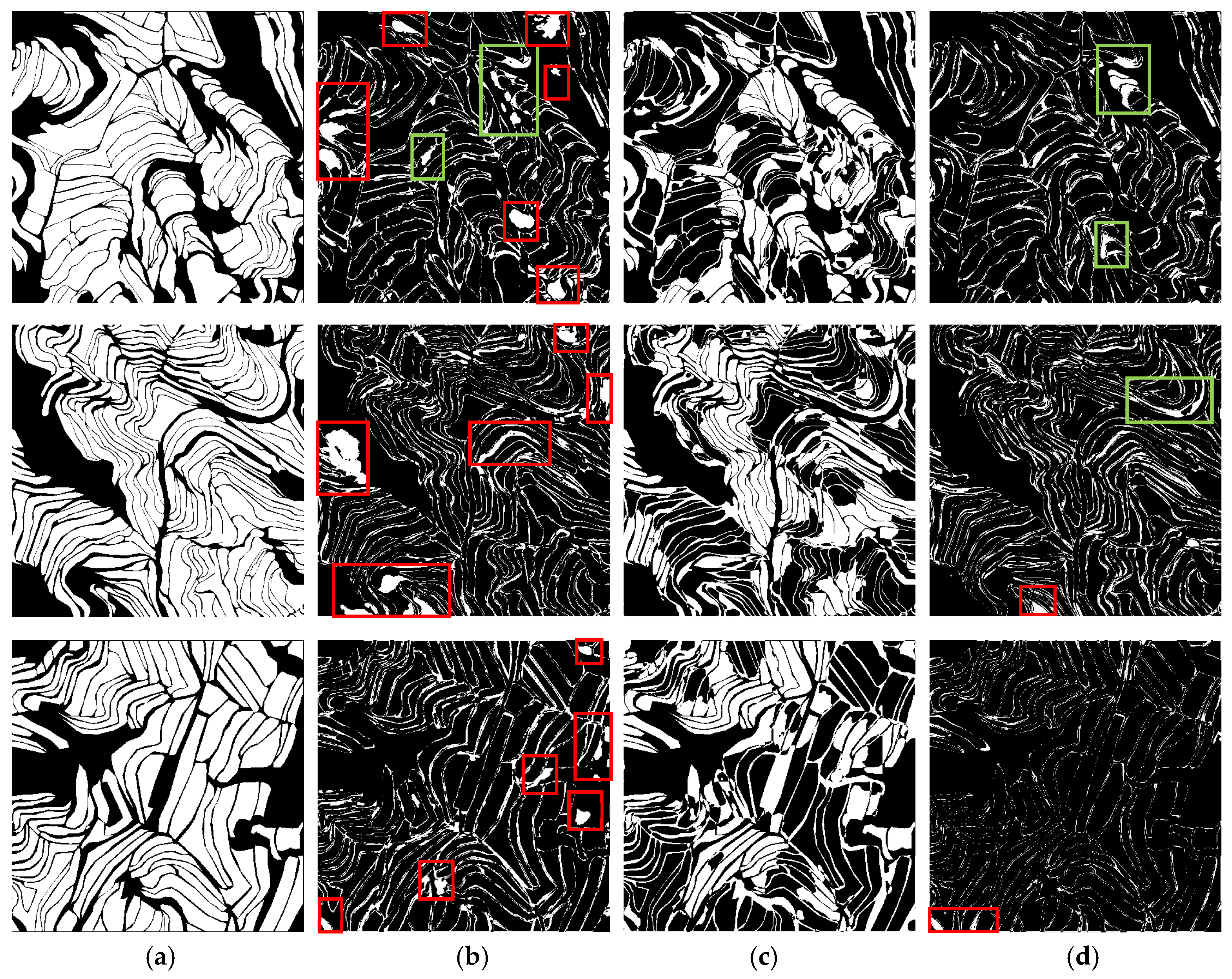
To evaluate the prediction results more objectively, this paper adopted two methods, namely visual interpretation and inter-frame background subtraction, to analyze the prediction results. In inter-frame background subtraction, the pixel value of the predicted result is subtracted from the pixel value of the real result to get a difference image. The difference images can help us to well-visualize the missing and misclassified parts. The difference images of the three methods in the three test areas are shown in Figure 14.
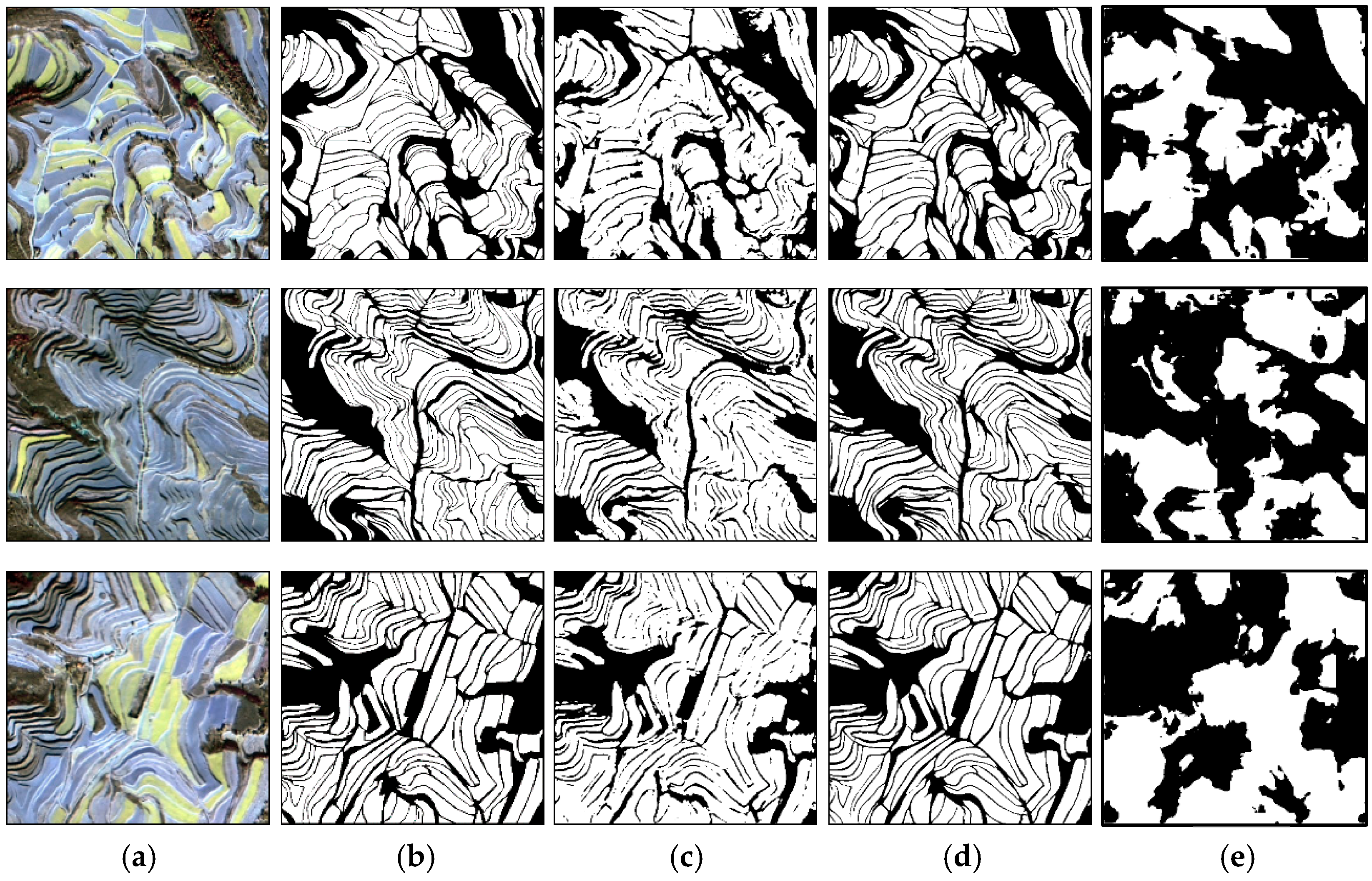
Figure 13 shows clearly that the transfer learning recognition method based on the second strategy performed the best. This method accurately identified the edges of the terraces and segmented the terrace fields. Although the direct training method successfully recognized terraces in a large area, the recognition of terrace edges was poor, the adhesion phenomenon was more serious, and greater problems involving missed and incorrect classification arose. In comparison, transfer learning based on the first strategy was the least effective. This method was unable to correctly identify the terraced field blocks and the edge lines. These results reveal that the transfer learning method that only trained linear classifiers saved a lot of training time compared to other methods, but it did not learn enough terrace features to well-identify the terraces.
When observing the difference images for the three test areas in Figure 14, we noted that the transfer learning method based on strategy 1 had the greatest white areas, which meant the missing and misclassified phenomena were serious. In addition, this method could hardly identify the terraced field boundaries. The red box in Figure 14 represents the misclassification area, that is, the misclassification of other types into terrace types. The green box in Figure 14, meanwhile, represents the missed classification areas, i.e., the unrecognized terraced areas. Figure 14 shows clearly that the overall recognition effect of the deep transfer learning method based on strategy 2 was better than that of the direct training method. This transfer learning method had only a few classification errors, while the direct training method had a serious misclassification problem. Both made errors in identifying terraced field boundaries; however, as shown in Figure 13, the deep transfer learning method based on strategy 2 could basically identify the boundaries, though the identified boundaries were wider than the real labels. The direct training method, meanwhile, poorly identified terrace boundaries, with most going unidentified.
In summary, both inter-frame background subtraction and the visual interpretation method show that the transfer learning method based on strategy 2—of using the weights of the pre-trained model to initialize the weights of the whole network and retrain the classifier—yielded excellent results in a recognition problem involving small-sample terraces. Another advantage of this method stems from being based on pre-trained model weights, and thus, requiring less training time than the direct training method.
After comparing the recognition results of the two methods, we calculated the confusion matrix based on the predicted results and the actual labels to complete the accuracy evaluation. Table 6 offers the accuracy evaluation results for the three test areas.
Table 6 indicates that the transfer learning method greatly improved the accuracy of each evaluation factor compared to the direct training method. The OA, F1 score, and MIoU in test area 1 increased by 7.21%, 13.67%, and 16.54%, in test area 2, by 10.11%, 15.44%, and 21.72%, and in test area 3, by 9.30%, 16.26%, and 20.56%, respectively. Overall, the average accuracy of the OA, F1 score, and MIoU in the three test areas increased by 8.88%, 15.12%, and 19.61%, respectively.
The comparison graphs and the results of our accuracy evaluation show that the transfer learning method was best at recognizing small-sample terraces and accurately segmenting the terrace surface. Its accuracy in terms of the three evaluation indexes was also the highest, with the average OA, F1 score, and MIoU reaching 93.12%, 91.40%, and 89.90% for the three test areas, respectively.
5. Conclusions and Future Research Direction
To solve the problem of how to quickly and accurately extract terraces from small-sample data, we proposed a precise pixel-level terrace extraction method from high-resolution remote-sensing images based on deep transfer learning. Accordingly, we constructed an optimal pre-training model for terrace recognition, as described in this paper. The superiority of transfer learning was verified by conducting a controlled trial with direct training. The training results for the GF-2 small-sample dataset showed that the transfer learning model offers better feature extraction and requires less training time. It can also better incorporate terrace edge information, segments the terrace surface more accurately, and solves the problem of how to adhere large, narrow terraces.
However, there were omissions from the outcomes of the model for terraces with smaller areas and a few misclassification issues arose. In addition, the terrace boundary information requires further improvement to its precision. A follow-up study will focus on the two following aspects:
- (1)
- Topographic characteristics data, such as DEM data, will be combined with high-resolution remote-sensing image data, on which we will use the deep learning method to obtain more accurate terrace extraction results.
- (2)
- A combination of transfer learning feature extraction and high-performance classifiers will be applied to explore whether the accuracy can be further improved, thereby bringing new insights to the field of terrace recognition.
Author Contributions
Conceptualization, M.Y. and X.R.; methodology, M.Y., X.R. and W.X.; software, X.X. and W.W.; validation, M.Y., X.R. and W.X.; formal analysis, X.R.; investigation, M.Y.; resources, X.X. and W.W.; data curation, M.Y., X.R. and W.W.; writing—original draft preparation, M.Y., X.R. and W.X.; writing—review and editing, M.Y. and X.R.; visualization, X.X. and W.W.; supervision, M.Y.; project administration, M.Y.; funding acquisition, M.Y. and X.R. All authors have read and agreed to the published version of the manuscript.
Funding
This paper was supported by the National Natural Science Foundation of China (Grant nos. U21A2011 and 40971129) and the Fundamental Research Funds for the Central Universities (grant no. 2019B02514).
Data Availability Statement
Not applicable.
Acknowledgments
All authors sincerely thank the reviewers for their beneficial, careful, and detailed comments and suggestions for how we could improve the paper.
Conflicts of Interest
The authors declare no conflict of interest.
References
- Rashid, M.; Rehman, O.; Alfonso, S.; Kausar, R.; Akram, M. The Effectiveness of Soil and Water Conservation Terrace Structures for Improvement of Crops and Soil Productivity in Rainfed Terraced System. Pakistan J. Agric. Sci. 2016, 53, 241–248. [Google Scholar] [CrossRef]
- Gardner, R.A.M.; Gerrard, A.J. Runoff and Soil Erosion on Cultivated Rainfed Terraces in the Middle Hills of Nepal. Appl. Geogr. 2003, 23, 23–45. [Google Scholar] [CrossRef]
- Capolupo, A.; Kooistra, L.; Boccia, L. A Novel Approach for Detecting Agricultural Terraced Landscapes from Historical and Contemporaneous Photogrammetric Aerial Photos. Int. J. Appl. Earth Obs. Geoinf. 2018, 73, 800–810. [Google Scholar] [CrossRef]
- Zhang, Y.; Shi, M.; Zhao, X.; Wang, X.; Luo, Z.; Zhao, Y. Methods for Automatic Identification and Extraction of Terraces from High Spatial Resolution Satellite Data (China-GF-1). Int. Soil Water Conserv. Res. 2017, 5, 17–25. [Google Scholar] [CrossRef] [Green Version]
- Liu, X.Y.; Yang, S.T.; Wang, F.G.; He, X.Z.; Ma, H.B.; Luo, Y. Analysis on Sediment Yield Reduced by Current Terrace and Shrubs-Herbs-Arbor Vegetation in the Loess Plateau. Shuili Xuebao/J. Hydraul. Eng. 2014, 45, 1293–1300. [Google Scholar] [CrossRef]
- Xiong, L.; Tang, G.; Yang, X.; Li, F. Geomorphology-Oriented Digital Terrain Analysis: Progress and Perspectives. Dili Xuebao/Acta Geogr. Sin. 2021, 76, 595–611. [Google Scholar] [CrossRef]
- Zhao, H.; Fang, X.; Ding, H.; Strobl, J.; Xiong, L.; Na, J.; Tang, G. Extraction of Terraces on the Loess Plateau from High-Resolution Dems and Imagery Utilizing Object-Based Image Analysis. ISPRS Int. J. Geo-Inf. 2017, 6, 157. [Google Scholar] [CrossRef] [Green Version]
- Pijl, A.; Quarella, E.; Vogel, T.A.; D’Agostino, V.; Tarolli, P. Remote Sensing vs. Field-Based Monitoring of Agricultural Terrace Degradation. Int. Soil Water Conserv. Res. 2021, 9, 1–10. [Google Scholar] [CrossRef]
- Martínez-Casasnovas, J.A.; Ramos, M.C.; Cots-Folch, R. Influence of the EU CAP on Terrain Morphology and Vineyard Cultivation in the Priorat Region of NE Spain. Land Use Policy 2010, 27, 11–21. [Google Scholar] [CrossRef]
- Agnoletti, M.; Cargnello, G.; Gardin, L.; Santoro, A.; Bazzoffi, P.; Sansone, L.; Pezza, L.; Belfiore, N. Traditional Landscape and Rural Development: Comparative Study in Three Terraced Areas in Northern, Central and Southern Italy to Evaluate the Efficacy of GAEC Standard 4.4 of Cross Compliance. Ital. J. Agron. 2011, 6, 121–139. [Google Scholar] [CrossRef]
- Zhao, B.Y.; Ma, N.; Yang, J.; Li, Z.H.; Wang, Q.X. Extracting Features of Soil and Water Conservation Measures from Remote Sensing Images of Different Resolution Levels: Accuracy Analysis. Bull. Soil Water Conserv. 2012, 32, 154–157. [Google Scholar] [CrossRef]
- Yu, H.; Liu, Z.-H.; Zhang, X.-P.; Li, R. Extraction of Terraced Field Texture Features Based on Fourier Transformation. Remote Sens. L. Resour. 2008, 20, 39–42. [Google Scholar]
- Zhao, X.; Wang, X.J.; Zhao, Y.; Luo, Z.D.; Xu, Y.L.; Guo, H.; Zhang, Y. A Feasibility Analysis on Methodology of Terraced Extraction Using Fourier Transformation Based on Domestic Hi-Resolution Remote Sensing Image of GF-1 Satellite. Soil Water Conserv. China 2016, 1, 63–65. [Google Scholar] [CrossRef]
- Luo, L.; Li, F.; Dai, Z.; Yang, X.; Liu, W.; Fang, X. Terrace Extraction Based on Remote Sensing Images and Digital Elevation Model in the Loess Plateau, China. Earth Sci. Informatics 2020, 13, 433–446. [Google Scholar] [CrossRef]
- Diaz-Varela, R.A.; Zarco-Tejada, P.J.; Angileri, V.; Loudjani, P. Automatic Identification of Agricultural Terraces through Object-Oriented Analysis of Very High Resolution DSMs and Multispectral Imagery Obtained from an Unmanned Aerial Vehicle. J. Environ. Manag. 2014, 134, 117–126. [Google Scholar] [CrossRef] [PubMed]
- Eckert, S.; Tesfay, S.G.; Hurni, H.; Kohler, T. Identification and Classification of Structural Soil Conservation Measures Based on Very High Resolution Stereo Satellite Data. J. Environ. Manag. 2017, 193, 592–606. [Google Scholar] [CrossRef] [PubMed] [Green Version]
- Hinton, G.E.; Salakhutdinov, R.R. Reducing the Dimensionality of Data with Neural Networks. Science 2006, 313, 504–507. [Google Scholar] [CrossRef] [Green Version]
- Krizhevsky, A.; Sutskever, I.; Hinton, G.E. ImageNet Classification with Deep Convolutional Neural Networks. Commun. ACM 2017, 60, 84–90. [Google Scholar] [CrossRef]
- Hamida, A.B.; Benoit, A.; Lambert, P.; Ben-Amar, C. Deep Learning Approach for Remote Sensing Image Analysis. In Proceedings of the Big Data from Space (BiDS’16), Santa Cruz de Tenerife, Spain, 15–17 March 2016. [Google Scholar]
- Gupta, S.; Dwivedi, R.K.; Kumar, V.; Jain, R.; Jain, S.; Singh, M. Remote Sensing Image Classification Using Deep Learning. In Proceedings of the 2021 10th International Conference on System Modeling and Advancement in Research Trends, SMART 2021, Moradabad, India, 10–11 December 2021. [Google Scholar]
- Cheng, G.; Yang, C.; Yao, X.; Guo, L.; Han, J. When Deep Learning Meets Metric Learning: Remote Sensing Image Scene Classification via Learning Discriminative CNNs. IEEE Trans. Geosci. Remote Sens. 2018, 56, 2811–2821. [Google Scholar] [CrossRef]
- Liu, P.; Choo, K.K.R.; Wang, L.; Huang, F. SVM or Deep Learning? A Comparative Study on Remote Sensing Image Classification. Soft Comput. 2017, 21, 7053–7065. [Google Scholar] [CrossRef]
- Huang, F.; Zhang, J.; Zhou, C.; Wang, Y.; Huang, J.; Zhu, L. A Deep Learning Algorithm Using a Fully Connected Sparse Autoencoder Neural Network for Landslide Susceptibility Prediction. Landslides 2020, 17, 217–229. [Google Scholar] [CrossRef]
- Do, H.T.; Raghavan, V.; Yonezawa, G. Pixel-Based and Object-Based Terrace Extraction Using Feed-Forward Deep Neural Network. ISPRS Ann. Photogramm. Remote Sens. Spat. Inf. Sci. 2019, 4, 1–7. [Google Scholar] [CrossRef] [Green Version]
- Zhao, F.; Xiong, L.Y.; Wang, C.; Wang, H.R.; Wei, H.; Tang, G.A. Terraces Mapping by Using Deep Learning Approach from Remote Sensing Images and Digital Elevation Models. Trans. GIS 2021, 25, 2438–3454. [Google Scholar] [CrossRef]
- Cook, D.; Feuz, K.D.; Krishnan, N.C. Transfer Learning for Activity Recognition: A Survey. Knowl. Inf. Syst. 2013, 36, 537–556. [Google Scholar] [CrossRef] [PubMed] [Green Version]
- Tang, J.; Shu, X.; Li, Z.; Qi, G.J.; Wang, J. Generalized Deep Transfer Networks for Knowledge Propagation in Heterogeneous Domains. ACM Trans. Multimed. Comput. Commun. Appl. 2016, 12, 68. [Google Scholar] [CrossRef]
- Lu, H.; Fu, X.; Liu, C.; Li, L.; He, Y.; Li, N. Cultivated Land Information Extraction in UAV Imagery Based on Deep Convolutional Neural Network and Transfer Learning. J. Mt. Sci. 2017, 14, 731–741. [Google Scholar] [CrossRef]
- Huang, Z.; Pan, Z.; Lei, B. Transfer Learning with Deep Convolutional Neural Network for SAR Target Classification with Limited Labeled Data. Remote Sens. 2017, 9, 907. [Google Scholar] [CrossRef] [Green Version]
- Kaya, A.; Keceli, A.S.; Catal, C.; Yalic, H.Y.; Temucin, H.; Tekinerdogan, B. Analysis of Transfer Learning for Deep Neural Network Based Plant Classification Models. Comput. Electron. Agric. 2019, 158, 20–29. [Google Scholar] [CrossRef]
- Tammina, S. Transfer Learning Using VGG-16 with Deep Convolutional Neural Network for Classifying Images. Int. J. Sci. Res. Publ. 2019, 9, 143–150. [Google Scholar] [CrossRef]
- Porter, C.C.; Morin, P.J.; Howat, I.M.; Niebuhr, S.; Smith, B.E. DEM Extraction from High-Resolution Stereoscopic Worldview 1 & 2 Imagery of Polar Outlet Glaciers. In Proceedings of the Fall Meeting of the American Geophysical Union, San Francisco, CA, USA, 5–9 December 2011. [Google Scholar]
- Li, P.; Yu, H.; Wang, P.; Li, K. Comparison and Analysis of Agricultural Information Extraction Methods Based upon GF2 Satellite Images. Bull. Surv. Mapp. 2017, 1, 48–52. [Google Scholar]
- Qin, Y.; Wu, Y.; Li, B.; Gao, S.; Liu, M.; Zhan, Y. Semantic Segmentation of Building Roof in Dense Urban Environment with Deep Convolutional Neural Network: A Case Study Using GF2 VHR Imagery in China. Sensors 2019, 19, 1164. [Google Scholar] [CrossRef] [PubMed] [Green Version]
- Ronneberger, O.; Fischer, P.; Brox, T. U-Net: Convolutional Networks for Biomedical Image Segmentation. In International Conference on Medical Image Computing and Computer-Assisted Intervention; Lecture Notes in Computer Science (Including Subseries Lecture Notes in Artificial Intelligence and Lecture Notes in Bioinformatics); Springer: Cham, Switzerland, 2015; Volume 9351. [Google Scholar]
- Shelhamer, E.; Long, J.; Darrell, T. Fully Convolutional Networks for Semantic Segmentation. IEEE Trans. Pattern Anal. Mach. Intell. 2017, 39, 640–651. [Google Scholar] [CrossRef] [PubMed]
- Feng, W.; Sui, H.; Huang, W.; Xu, C.; An, K. Water Body Extraction from Very High-Resolution Remote Sensing Imagery Using Deep U-Net and a Superpixel-Based Conditional Random Field Model. IEEE Geosci. Remote Sens. Lett. 2019, 16, 618–622. [Google Scholar] [CrossRef]
- Srivastava, N.; Hinton, G.; Krizhevsky, A.; Sutskever, I.; Salakhutdinov, R. Dropout: A Simple Way to Prevent Neural Networks from Overfitting. J. Mach. Learn. Res. 2014, 15, 1929–1958. [Google Scholar]
- Ioffe, S.; Szegedy, C. Batch Normalization: Accelerating Deep Network Training by Reducing Internal Covariate Shift. In Proceedings of the 32nd International Conference on Machine Learning, ICML 2015, Lille, France, 6–11 July 2015; Volume 1, pp. 448–456. [Google Scholar]
- Wang, Z.; Zhou, Y.; Wang, S.; Wang, F.; Xu, Z. House Building Extraction from High-Resolution Remote Sensing Images Based on IEU-Net. Yaogan Xuebao/J. Remote Sens. 2021, 25, 2245–2254. [Google Scholar] [CrossRef]
- Glorot, X.; Bordes, A.; Bengio, Y. Deep Sparse Rectifier Neural Networks. In Proceedings of the JMLR Workshop and Conference Proceedings, Lauderdale, FL, USA, 11–13 April 2011; pp. 315–323. [Google Scholar]
- Pan, S.J.; Yang, Q. A Survey on Transfer Learning. IEEE Trans. Knowl. Data Eng. 2010, 22, 1345–1359. [Google Scholar] [CrossRef]
- Keskar, N.S.; Nocedal, J.; Tang, P.T.P.; Mudigere, D.; Smelyanskiy, M. On Large-Batch Training for Deep Learning: Generalization Gap and Sharp Minima. In Proceedings of the 5th International Conference on Learning Representations, ICLR 2017—Conference Track Proceedings, Toulon, France, 24–26 April 2017. [Google Scholar]
- Hoffer, E.; Hubara, I.; Soudry, D. Train Longer, Generalize Better: Closing the Generalization Gap in Large Batch Training of Neural Networks. In Proceedings of the Advances in Neural Information Processing Systems, Long Beach, CA, USA, 4–9 December 2017; Volume 2017. [Google Scholar]
- Smith, S.L.; Kindermans, P.J.; Ying, C.; Le, Q.V. Don’t Decay the Learning Rate, Increase the Batch Size. In Proceedings of the 6th International Conference on Learning Representations, ICLR 2018—Conference Track Proceedings, Vancouver, BC, Canada, 30 April 30–3 May 2018. [Google Scholar]
Figure 1.
Geographic location of the study area and regional remote-sensing images.

Figure 2.
Schematic diagram of overlapping sliding window cropping. The yellow box is the sliding window, 256 × 256 pixels in size. The yellow arrow is the sliding track. The red area is the overlapping area.
Figure 2.
Schematic diagram of overlapping sliding window cropping. The yellow box is the sliding window, 256 × 256 pixels in size. The yellow arrow is the sliding track. The red area is the overlapping area.

Figure 3.
WorldView-1 sample set of fused images and their corresponding labels. The top row shows the WorldView-1 sample set of fused images. The bottom row represents the true labels corresponding to the WorldView-1 sample set of fused images.
Figure 3.
WorldView-1 sample set of fused images and their corresponding labels. The top row shows the WorldView-1 sample set of fused images. The bottom row represents the true labels corresponding to the WorldView-1 sample set of fused images.

Figure 4.
GF-2 sample set of fused images and their corresponding labels. The top row shows the GF-2 sample set of fused images. The bottom row represents the true labels corresponding to the GF-2 sample set of fused images.
Figure 4.
GF-2 sample set of fused images and their corresponding labels. The top row shows the GF-2 sample set of fused images. The bottom row represents the true labels corresponding to the GF-2 sample set of fused images.

Figure 5.
Fusion image of GF-2 sample area and fusion images of three test areas outside the sample area. (a) Sample area image; (b) test area 1 image; (c) test area 2 image; (d) test area 3 image. The sample area image is 3400 × 3400 pixels in size. The test area 1, 2, and 3 images are all 500 × 500 pixels in size.

Figure 6.
Range and distribution of the WorldView-1 and GF-2 images after fusion, and the geographic spacing of the GF-2 test area and sample area. The largest image in the figure is the fused WorldView-1 sample area. The medium image in the figure is the fused GF-2 sample area. The three smallest images in the figure are the fused GF-2 test area images.

Figure 7.
Flow chart of the method applied in this paper.

Figure 8.
IELoss calculation area diagram. Blue region is the loss value calculation area of the IEU-Net model. White region A is the loss value calculation area of a traditional U-Net model.
Figure 8.
IELoss calculation area diagram. Blue region is the loss value calculation area of the IEU-Net model. White region A is the loss value calculation area of a traditional U-Net model.

Figure 9.
Feature-mapping maps of 10 convolutional layers of the input image. Conv1-1 and Conv1-2 are the feature maps for the two convolutional layers of the first set of convolutional operations, and so on.
Figure 9.
Feature-mapping maps of 10 convolutional layers of the input image. Conv1-1 and Conv1-2 are the feature maps for the two convolutional layers of the first set of convolutional operations, and so on.

Figure 10.
Diagram of pooling operation.

Figure 11.
Diagram of prediction method. The size of A should be consistent with the size of the sample image, which is 256 × 256 pixels in this paper.
Figure 11.
Diagram of prediction method. The size of A should be consistent with the size of the sample image, which is 256 × 256 pixels in this paper.

Figure 12.
Accuracy and loss graphs for the training and validation datasets. (a) Pre-trained model’s training and validation datasets’ accuracy graph; (b) Pre-trained model’s training and validation datasets’ loss graph; (c) Transfer learning model’s training and validation datasets’ accuracy graph; (d) Transfer learning model’s training and validation datasets’ loss graph. The horizontal axis indicates the number of iterations and the vertical axis indicates the accuracy or loss value.

Figure 13.
Comparison of terrace identification results in the test area. (a) Test images; (b) true labels; (c) direct training prediction images; (d) transfer learning strategy 2 prediction images; (e) transfer learning strategy 1 prediction images. The top, middle, and bottom rows are the prediction images for test areas 1, 2, and 3, respectively.

Figure 14.
Difference images for the three methods in the three test areas. (a) True labels; difference images for (b) direct training methods, (c) transfer learning strategy 1, and (d) transfer learning strategy 2. The top, middle, and bottom rows are the difference images for test areas 1, 2, and 3, respectively. The white areas are the parts where the predicted results are different from the real labels. The black areas are the parts where the predicted results are the same as the real labels.


Table 1.
WorldView-1 satellite image parameters.
| Image Type | Band | Spectral Range (μm) | Spatial Resolution (m) |
|---|---|---|---|
| panchromatic image | PAN | 0.40~0.90 | 0.5 1 |
1 For non-government users, the image must be resampled to 0.5 m.
Table 2.
GF-2 satellite image parameters.
| Image Type | Band | Spectral Range (μm) | Spatial Resolution (m) |
|---|---|---|---|
| panchromatic image | PAN | 0.40~0.90 | 0.8 |
| multispectral image | B1 | 0.45~0.52 | 3.2 |
| B2 | 0.52~0.59 | ||
| B3 | 0.63~0.69 | ||
| B4 | 0.77~0.89 |
Table 3.
The structure and number of parameters of the IEU-Net.
| Layer (Number) | Layer (Type) | Output Shape | Parameter No. |
|---|---|---|---|
| 1 | input_1 | (None, 256, 256, 3) | 0 |
| 2 | conv2d | (None, 256, 256, 32) | 896 |
| 3 | batch_normalization | (None, 256, 256, 32) | 128 |
| 4 | conv2d_1 | (None, 256, 256, 32) | 9248 |
| 5 | batch_normalization_1 | (None, 256, 256, 32) | 128 |
| 6 | max_pooling2d | (None, 128, 128, 32) | 0 |
| … | … | … | … |
| … | … | … | … |
| 23 | conv2d_8 | (None, 16, 16, 512) | 1,180,160 |
| 24 | batch_normalization_8 | (None, 16, 16, 512) | 2048 |
| 25 | conv2d_9 | (None, 16, 16, 512) | 2,359,808 |
| 26 | batch_normalization_9 | (None, 16, 16, 512) | 2048 |
| 27 | dropout_1 | (None, 16, 16, 512) | 0 |
| 28 | up_sampling2d | (None, 32, 32, 512) | 0 |
| 29 | conv2d_10 | (None, 32, 32, 512) | 1,049,088 |
| 30 | concatenate | (None, 32, 32, 768) | 0 |
| … | … | … | … |
| … | … | … | … |
| 52 | conv2d_20 | (None, 256, 256, 32) | 18,464 |
| 53 | batch_normalization_16 | (None, 256, 256, 32) | 128 |
| 54 | conv2d_21 | (None, 256, 256, 32) | 9248 |
| 55 | batch_normalization_17 | (None, 256, 256, 32) | 128 |
| 56 | conv2d_22 | (None, 256, 256, 2) | 578 |
| 57 | conv2d_23 | (None, 256, 256, 2) | 6 |
Table 4.
Specific parameters.
| Epoch | Batch Size | Learning Rate | Optimizer |
|---|---|---|---|
| 100 | 16 | 1 × 10⁻⁴ | Adam |
Table 5.
Confusion matrix of prediction results.
| Prediction Type | Real Type | |
|---|---|---|
| Terraces | Non-Terraced Fields | |
| Terraces | TP (True Positives) | FP (False Positives) |
| Non-terraced fields | FN (False Negatives) | TN (True Negatives) |
Table 6.
Precision evaluation results.
| Test area | OA (%) | F1 Score (%) | MIoU (%) | |||
|---|---|---|---|---|---|---|
| Direct Training | Transfer Learning | Direct Training | Transfer Learning | Direct Training | Transfer Learning | |
| 1 | 84.41 | 91.62 | 77.50 | 91.17 | 70.97 | 87.51 |
| 2 | 83.06 | 93.17 | 74.02 | 89.46 | 68.22 | 89.94 |
| 3 | 85.26 | 94.56 | 77.32 | 93.58 | 71.68 | 92.24 |
Publisher’s Note: MDPI stays neutral with regard to jurisdictional claims in published maps and institutional affiliations. |
© 2022 by the authors. Licensee MDPI, Basel, Switzerland. This article is an open access article distributed under the terms and conditions of the Creative Commons Attribution (CC BY) license (https://creativecommons.org/licenses/by/4.0/).
Share and Cite
MDPI and ACS Style
Yu, M.; Rui, X.; Xie, W.; Xu, X.; Wei, W. Research on Automatic Identification Method of Terraces on the Loess Plateau Based on Deep Transfer Learning. Remote Sens. 2022, 14, 2446. https://0-doi-org.brum.beds.ac.uk/10.3390/rs14102446
AMA Style
Yu M, Rui X, Xie W, Xu X, Wei W. Research on Automatic Identification Method of Terraces on the Loess Plateau Based on Deep Transfer Learning. Remote Sensing. 2022; 14(10):2446. https://0-doi-org.brum.beds.ac.uk/10.3390/rs14102446
Chicago/Turabian StyleYu, Mingge, Xiaoping Rui, Weiyi Xie, Xijie Xu, and Wei Wei. 2022. "Research on Automatic Identification Method of Terraces on the Loess Plateau Based on Deep Transfer Learning" Remote Sensing 14, no. 10: 2446. https://0-doi-org.brum.beds.ac.uk/10.3390/rs14102446
Note that from the first issue of 2016, this journal uses article numbers instead of page numbers. See further details here.