
PFD-SLAM: A New RGB-D SLAM for Dynamic Indoor Environments Based on Non-Prior Semantic Segmentation


1
School of Civil Engineering and Architecture, Changzhou Institute of Technology, Changzhou 213032, China
2
School of Geographic and Biologic Information, Nanjing University of Posts and Telecommunications, Nanjing 210023, China
3
School of Communications and Information Engineering, Nanjing University of Posts and Telecommunications, Nanjing 210023, China
4
Institute of Robotics and Autonomous Systems, School of Electrical and Information Engineering, Tianjin University, Tianjin 300072, China
5
School of Earth Science and Engineering, Hohai University, Nanjing 211000, China
*
Author to whom correspondence should be addressed.
Remote Sens. 2022, 14(10), 2445; https://0-doi-org.brum.beds.ac.uk/10.3390/rs14102445
Submission received: 6 April 2022
/
Revised: 8 May 2022
/
Accepted: 18 May 2022
/
Published: 19 May 2022
(This article belongs to the Special Issue Computer Vision and Image Processing)
Abstract
:Now, most existing dynamic RGB-D SLAM methods are based on deep learning or mathematical models. Abundant training sample data is necessary for deep learning, and the selection diversity of semantic samples and camera motion modes are closely related to the robust detection of moving targets. Furthermore, the mathematical models are implemented at the feature-level of segmentation, which is likely to cause sub or over-segmentation of dynamic features. To address this problem, different from most feature-level dynamic segmentation based on mathematical models, a non-prior semantic dynamic segmentation based on a particle filter is proposed in this paper, which aims to attain the motion object segmentation. Firstly, GMS and optical flow are used to calculate an inter-frame difference image, which is considered an observation measurement of posterior estimation. Then, a motion equation of a particle filter is established using Gaussian distribution. Finally, our proposed segmentation method is integrated into the front end of visual SLAM and establishes a new dynamic SLAM, PFD-SLAM. Extensive experiments on the public TUM datasets and real dynamic scenes are conducted to verify location accuracy and practical performances of PFD-SLAM. Furthermore, we also compare experimental results with several state-of-the-art dynamic SLAM methods in terms of two evaluation indexes, RPE and ATE. Still, we provide visual comparisons between the camera estimation trajectories and ground truth. The comprehensive verification and testing experiments demonstrate that our PFD-SLAM can achieve better dynamic segmentation results and robust performances.
1. Introduction
Nowadays, indoor navigation and positioning is an important constituent section and research hotspot in the fields of location-based services, which has attracted extensive attention from the government, industry, and academia [1,2]. How does the robot realize autonomous navigation and positioning? Simultaneous localization and mapping (SLAM) has been a primary key solution for the autonomous position of robots in unknown scenes and has become an active research field in the recent decade [3]. The early SLAM scheme relies on routine ranging sensors (e.g., radar, laser rangefinder, sonar) as data input. Compared to the ranging instruments mentioned above, visual cameras, which have inherent advantages of smaller size and lower cost and power consumption, can provide abundant texture and geometric information. The SLAM algorithms that utilize camera images as the input data source are named visual SLAM. With the tremendous development of computer vision, the visual SLAM community has attracted extensive concerns and been applied successfully to some specific fields, including deep space exploration [4], VR (virtual reality) [5], autonomous driving [6], etc.
Over the past few decades, several state-of-the-art SLAM algorithms (e.g., ORB-SLAM2 [7], DVO-SLAM [8], VINS-Mono [9]) have been issued. They could gain robust performances and comparable location accuracy in the static scenes. However, moving objects, such as walking humans, exist frequently in real-life scenarios. When some vision features are from dynamic objects, the wrong data association will occur and limit the usages of most excellent visual SLAM algorithms. If some matched features involve data correlation with dynamic objects, it inevitably leads to the accuracy degradation of camera pose estimation or even feature-tracking failure. Meanwhile, most visual SLAM algorithms cannot detect and reject dynamic elements, which are extremely restricted in dynamic scenes. Accordingly, more relevant research on visual SLAM for dynamic scenes has attracted extensive concern in recent years.
Visual SLAM methods aiming at dynamic settings have been proposed to improve robustness and accuracy. Generally speaking, these dynamic SLAMs are approximately divided into two categories: the basis of deep learning or a mathematical model. Deep learning embedded in dynamic SLAM systems is mainly used to segment prior semantic information. The robust or weak prior semantic segmentation effect is closely related to the accuracy of camera pose estimation. Moreover, an appropriate deep learning model needs to select and train a mass of data samples in advance, and the diversity of samples closely affects the generalization of semantic segmentation and practical performances. Another kind of dynamic SLAM method based on mathematical models is often prone to over or less segmentation of motion elements occurring, resulting in losses of mass static image features. Furthermore, most existing dynamic SLAMs combined with mathematical models usually attain the feature-level segmentation of moving objects. The judgment and recognition precision of dynamic features is the key to improving the accuracy of camera position estimation. Therefore, to address the problems mentioned above, in the paper, a mathematical segmentation approach based on both the particle filter and depth image is proposed. Then, our segmentation model is integrated into the front end of visual SLAM, establishing a new SLAM scheme, abbreviated as PFD-SLAM.
As dynamic features generally affect the robustness of pose estimation between frames, we apply the sparse optical flow and epipolar constraint to filter out these dynamic point features primitively. First, to acquire the robust matching pairs between adjacent frames, the matching algorithm of GMS (Grid-based Motion Statistics) [10] is utilized to obtain as many matched points as possible. Then, the nonlinear model describing the transformation relation between adjacent frames, namely homography, is discussed. The transformation model mentioned here provides observation information for the posterior probability estimation based on a particle filter. Gaussian distribution is applied to establish a motion model of each particle point. After accomplishing these preparations, the depth images and tracking convergence results of particle points are employed together to segment specific dynamic objects. It is essentially distinguished from dynamic feature-level recognition based on most mathematical models. What is more, while conducting the segmentation of moving objects, our segmentation method does not demand pre-training samples, in comparison with most prior semantic information segmentation algorithms dependent on the deep learning models. Therefore, we call our proposed method non-prior semantic segmentation, which improves the generalization performance of semantic segmentation to some extent. Finally, by extracting these visual features in the remaining region of RGB images, a camera pose is optimized by static visual feature elements. The main contributions of our work are summarized as follows:
- We proposed a new motion object segmentation mathematical model based on non-prior information, which was combined with depth images and a particle filter. The segmentation method first applied GMS and optical flow to obtain robust matching pairs of point features. Then, the depth image and particle filter were jointly used to segment dynamic objects in the indoor scene.
- We integrated the motion segmentation method into the front end of SLAM and adopted the remaining static region on RGB images to achieve higher accuracy of pose estimation and robustness performances in dynamic scenes. Thus, a new RGB-D SLAM method for dynamic indoor environments, called PFD-SLAM, was established.
- We evaluated our PFD-SLAM on the public TUM (Technical University of Munich) RGB-D datasets [11], which contained typical dynamic scene sequences, and the data sequences captured in real dynamic scenes [12]. Compared to these state-of-the-art dynamic visual SLAM algorithms, PFD-SLAM outperformed the performance of most dynamic SLAMs and achieved comparable accuracy.
The rest of the paper is organized as follows. Section 2 presents a review of related work. Section 3 describes the details of PFD-SLAM. The experimental results demonstrated on the TUM datasets and real scene sequences are shown in Section 4. Finally, the discussion and conclusion are given in Section 5 and Section 6.
2. Related Works
In this section, we review several excellent representative dynamic SLAM algorithms. There are roughly two kinds of dynamic feature-processing methods: segmentation of moving objects based on deep learning or the detection of dynamic features via a non-deep learning model [13]. In the paper, these segmentation methods through deep learning are classified as prior semantic segmentation models, while the latter categories are regarded as non-prior semantic information-based models. The remarkable distinction is whether the acquisition of segmentation results in dynamic objects are dependent on the prior segmentation semantic information or not. These details of each category are discussed in Section 2.1 and Section 2.2.
2.1. Dynamic SLAM Based on Non-Prior Semantic Information
The basic motivation of dynamic SLAM was to judge and eliminate motion features correctly in the dynamic scene. The first SLAM algorithm fusing motion object tracking was proposed in 2002, and the detection method included a consistency-based approach and a dynamic object map-based approach [14]. Then, extensive similar efforts [15,16,17,18] for dynamic object detection were raised gradually. The epipolar constraint [19] and optical flow [20] were usually combined to determine dynamic features. The geometry constraint mainly depended on a fundamental matrix constraint or an essential matrix constraint. As the methods mentioned above only attained results of dynamic features, other approaches for dynamic segmentation were proposed [15,16]. A motion removal model [17] combined Maximum Posterior Estimation (MPE) with K-Means clustering to segment dynamic objects. Other mathematical segmentation methods, for instance, dense scene flow [21] or estimating static background [18], could achieve dynamic object segmentation. In real dynamic scenes, as the camera is in motion, due to its irregular motion modes or time-varying motion of dynamic objects, in the process of dynamic features recognition and segmentation, these factors lead such segmentation models to generally give rise to over or sub-segmentation, which generate wrong data associations and poor performances eventually.
To ensure robust identification results, sometimes some additional sensors are complementary to detect and eliminate dynamic point features more efficiently and conveniently. Zou et al. [22] applied a group of monocular cameras to distinguish whether these point features were static or dynamic according to the re-projection error of matches point features and the field angle of cameras. Liu et al. [23] detected and rejected outlier feature points based on different view fields of RGB-D sensors and the GMS matching algorithm. As the inertial measurement unit (IMU) was insensitive to external dynamic features, it was applied to the detection and elimination of dynamic point features. Kim et al. [24] utilized an RGB-D camera and IMU to perform the dynamic SLAM. The measurement information of IMU was being utilized as prior information to eliminate wrong data associations in the dynamic scene. In general, the complementary modalities could effectively address localization problems in dynamic environments, but the multi-sensor calibration and combination process increased the implementation difficulty.
2.2. Dynamic SLAM Based on Prior Semantic Information
With the rapid development of deep learning, deep learning based on the convolutional neural network could segment semantic information accurately. Most robust SLAMs aiming at dynamic scenes combined with deep learning have been proposed to improve performance remarkably. Bescos [25] was the first to combine the convolutional neural network-Mask R-CNN [26] and multi-view geometry to determine whether dynamic segmentation results were moving or not and proposed the Dyna-SLAM with an open-source code. Due to the accuracy and efficiency of semantic segmentation based on deep learning, the SLAM method combined with it has gradually become a mainstream method in the dynamic SLAM community. Zhang [27] also applied the Mask R-CNN to construct a dynamic RGB-D SLAM. He used the convolutional neural network to detect semantic information and estimated the possibility of dynamic or static parts. Due to a lack of judgment and determination of dynamic features, the proposed method in [27] removed the possible dynamic semantic information merely. Yu et al. [28] applied the SegNet network to obtain a pixel-wise semantic segmentation of images and combined it with a motion consistency checking strategy to filter out dynamic portions of the scene. Yu [28] also produced a dense semantic octree map, which is helpful to further deepen the understanding and mapping of dynamic scenes. Based on semantic information, Cui [29] integrated the optical flow into the RGB-D mode of ORB-SLAM2 to present SOF-SLAM, Semantic Optical Flow SLAM, a visual semantic SLAM system toward the dynamic environment. This semantic optical flow was a kind of tightly coupled approach, and it can fully take advantage of features’ dynamic characteristics hidden in semantic and geometry information to remove dynamic features more effectively and reasonably. Similar to the work of [29], Han [30] also combined a PSPnet semantic network and optical flow to identify moving objects in dynamic scene sequences as soon as possible.
As an RGB-D camera can provide RGB and depth images simultaneously, except for the dynamic SLAM fusing deep learning directly, several significant proposals combine semantic information from deep learning and depth information to filter out dynamic features [31,32,33,34]. On the basis of ORB-SLAM2, Yuan [31] determined the dynamic objects by combining the depth value of an RGB-D camera and semantic information to find out feature points that belong to movable objects. They detect whether those feature points are keeping still at the moment and achieve excellent performance in dynamic environments. Cui [32] utilized the depth and semantic information to construct depth filters and finally perform the detection of moving objects. Similar to the work of [16], Cheng [12] applied semantic information and achieved the update of dynamic label information based on a Bayesian filter. Ran et al. [33] combined the semantic information and Bayesian update to present a robust RS-SLAM, which could detect moving and movable objects. Cheng [34], based on previous work [12,20], proposed a SLAM framework, which achieved the 3D reconstruction of dynamic scenes and recorded trajectories of human activity.
Generally speaking, these dynamic SLAM schemes, which are based on deep learning, can achieve a higher positioning accuracy. Before applying deep learning to segment semantic information, the selection and training of data samples need to be finished in advance. The shortage of sample diversity will weaken the segmentation ability of the trained convolutional neural network model, and it may lead to the incomplete segmentation of semantic information or wrong associations, which cause the degradation of camera pose estimation. In addition, most motion feature segmentations based on mathematical models are prone to cause over-elimination of dynamic features, which will lead to the loss of partial static features and the precision degradation of SLAM and even tracking failure eventually. Therefore, to avoid the sub-over semantic segmentation case within most mathematical models or the weak segmentation generalization of deep learning, we proposed a dynamic object segmentation approach based on particle filters and depth images and then fused the model into the front end of SLAM by constituting PFD-SLAM to attain better performances in the indoor dynamic scenes.
3. Methodology
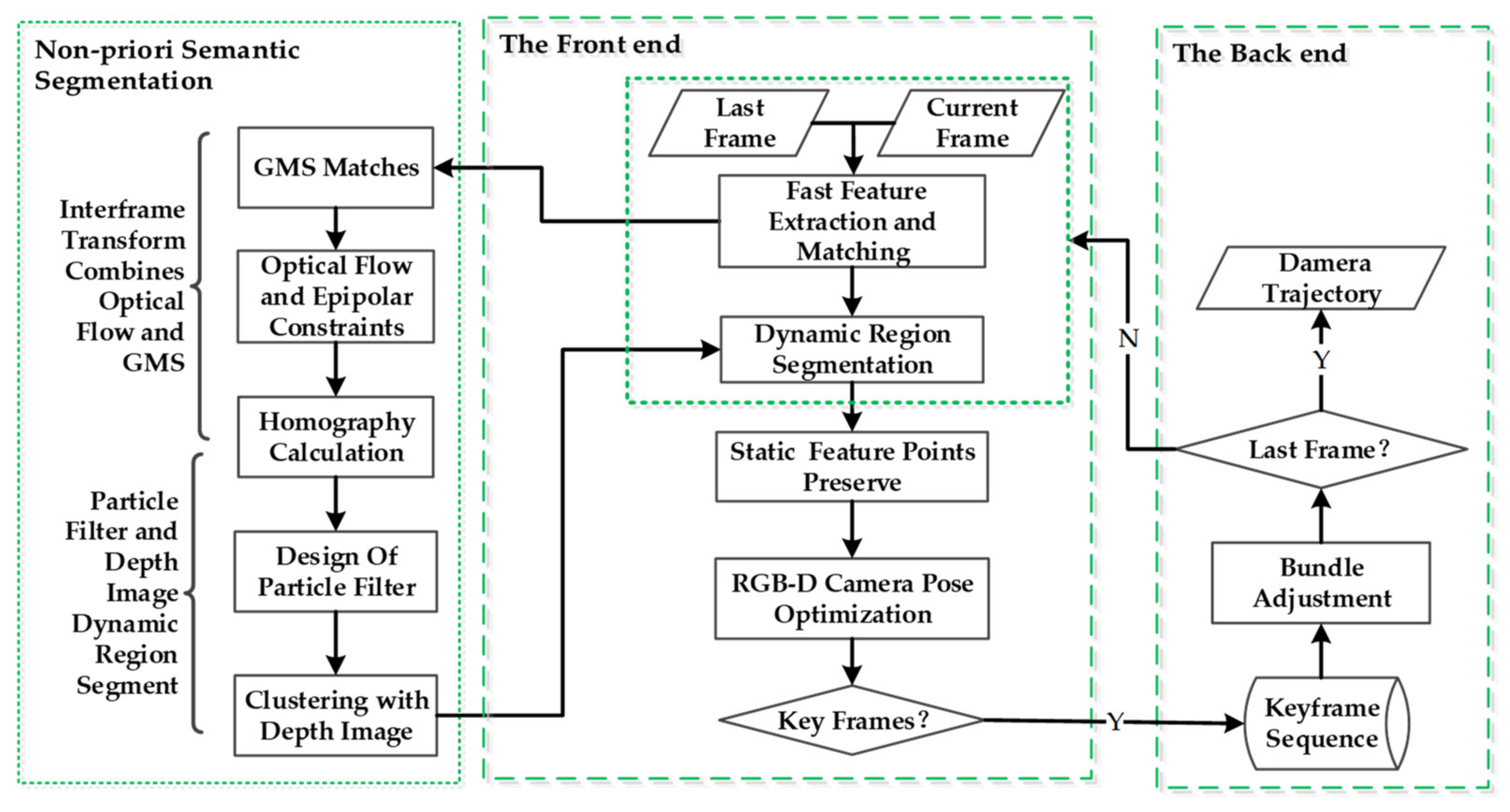
In this section, our proposed dynamic segmentation method based on posterior probability estimation and an RGB-D camera will be described systematically. After completing the segmentation of dynamic objects, the obtained static region is integrated into the front end of PFD-SLAM. In the back end, bundle adjustment is executed to reduce the drift of estimated camera trajectories. When bundle adjustment is accomplished, PFD-SLAM will determine and judge whether the current frame is the last frame or not. If so, the camera trajectory is output. The overall procedure of our proposed non-prior semantic information segmentation and PFD-SLAM is given in Figure 1.
3.1. Inter-Frame Transformation Combining Optical Flow and GMS
The basic idea of the GMS matching algorithm is to apply statistical theory to determine whether matching pairs are correct or not. If the number of neighborhood feature matches is dominant, the matching pairs will more likely be the corrected one. According to the Bayes rule, if there are many matching supporting relationships in the neighborhood of the matching pair, the matches are likely to be true. When the number of supported neighborhoods is more significant than a preset threshold, the current matching pair will be correctly matched.
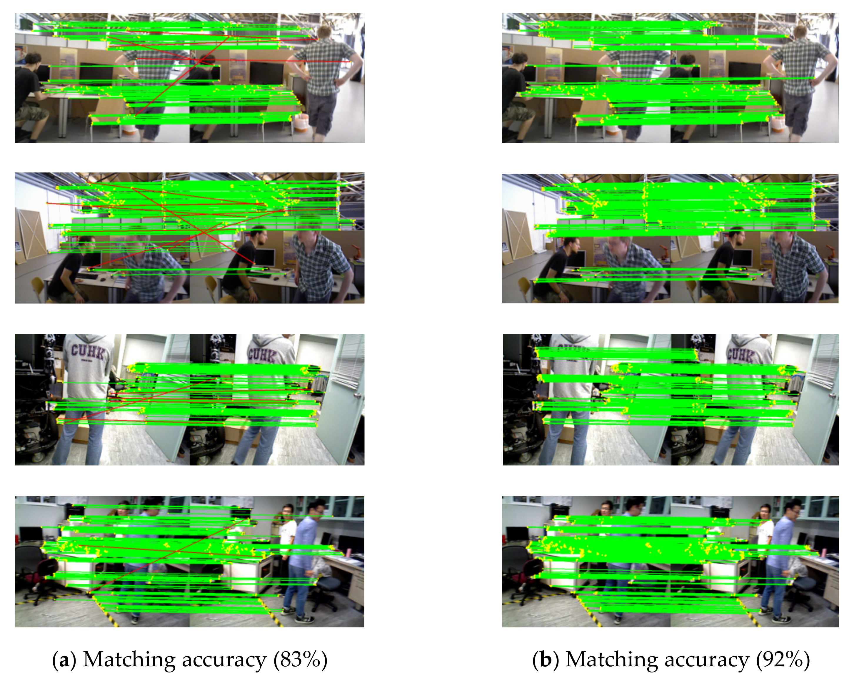
To the interference from dynamic features, the feature matching results obtained by the RANSAC algorithm [35] are not quite reliable, and the mismatch also easily occurs in the dynamic scenes. Figure 2 shows the matched result using two different matching algorithms. In Figure 2, (a) gives the feature matching result by combining with BF-Matcher and RANSAC, while (b) displays a corresponding result acquired from the GMS algorithm. By comparing the matching results given in Figure 2, it can be intuitively found that these feature match pairs of the GMS algorithm have no apparent mismatches. In contrast, in the former matching result some mismatched point pairs with weaker robustness exist.
In real dynamic scenes, as the motion modes of a camera involve vast translation and rotation components, sometimes it makes the images irregular and makes some affine linear models [36] challenging to describe the corresponding pixel mapping relationship of adjacent frames accurately. In the paper, the homography transformation, a nonlinear model, is applied to formulate the corresponding relation in adjacent frames, and the homography matrix can be directly calculated using the remaining matched points. The diversity and complexity of motion styles within dynamic objects in real scenes will affect the robustness and accuracy of the homography matrix calculation typically. It is known that optical flow can recognize dynamic features, coupled with the robustness of the GMS algorithm. This section proposes to combine the sparse optical flow with GMS algorithms to calculate the transformation of adjacent frames.
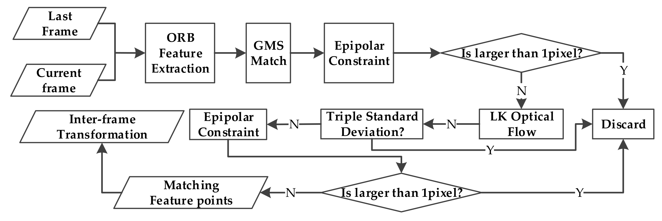
Figure 3 shows the calculation steps of the inter-frame transformation based on optical flow and the GMS algorithm. Firstly, fast corner points in adjacent frames are extracted, and feature points are matched using the GMS algorithm. Meanwhile, a fundamental matrix is calculated, and outlier feature points are detected and discarded by the epipolar constraints initially. According to our rich practical experience and test verification results, the threshold from a feature point to an epipolar line is set as 1 pixel to remove dynamic points accurately. Then, the L-K (Lucas-Kanade) sparse optical flow is used to track the remaining feature points. The variance and mean square error of the 2D coordinate difference between the feature matching points and corresponding tracking points are calculated statistically. Based on error theory and surveying adjustment, the index of triple standard deviation is considered as the tolerance error to determine these dynamic points. The triple standard deviation of the point coordinate difference is regarded as the threshold, which is a criterion for discerning and rejecting the dynamic feature points tracked by the optical flow algorithm. Finally, to filter dynamic features more precisely, the matching pairs that are greater than 1 pixel are removed by applying the epipolar constraint again. After fulfilling the steps above, the remnant feature points are used to calculate the transformation relationship of frames. The transformation relation not only can avoid the interference of dynamic features, but also ensure the robustness of the proposed solution. The specific calculation steps are shown as follows Algorithm 1:
| Algorithm 1: The transformation of the inter-frame based on the optical flow and GMS |
| Input: Last Frame Flast, Current Frame Fcurr |
| Output: The transformation relationship H |
| 0: Extraction ORB Fast feature points in Flast and Fcurr; |
| 1: GMS→the feature matches collection M; |
| 2: Fundamental Matrix and RANSAC→reject outlier points and update M′; |
| 3: goodFeaturesToTrack→tracking the remaining features; |
| 4: Computing LK optical flow→remove outlier feature points and update M′; |
| 5: for each point in M′ |
| if the related epipolar constraint distance >1 pixel, delete; else, reserve in M″; |
| end |
| 6: M″→calculation H; |
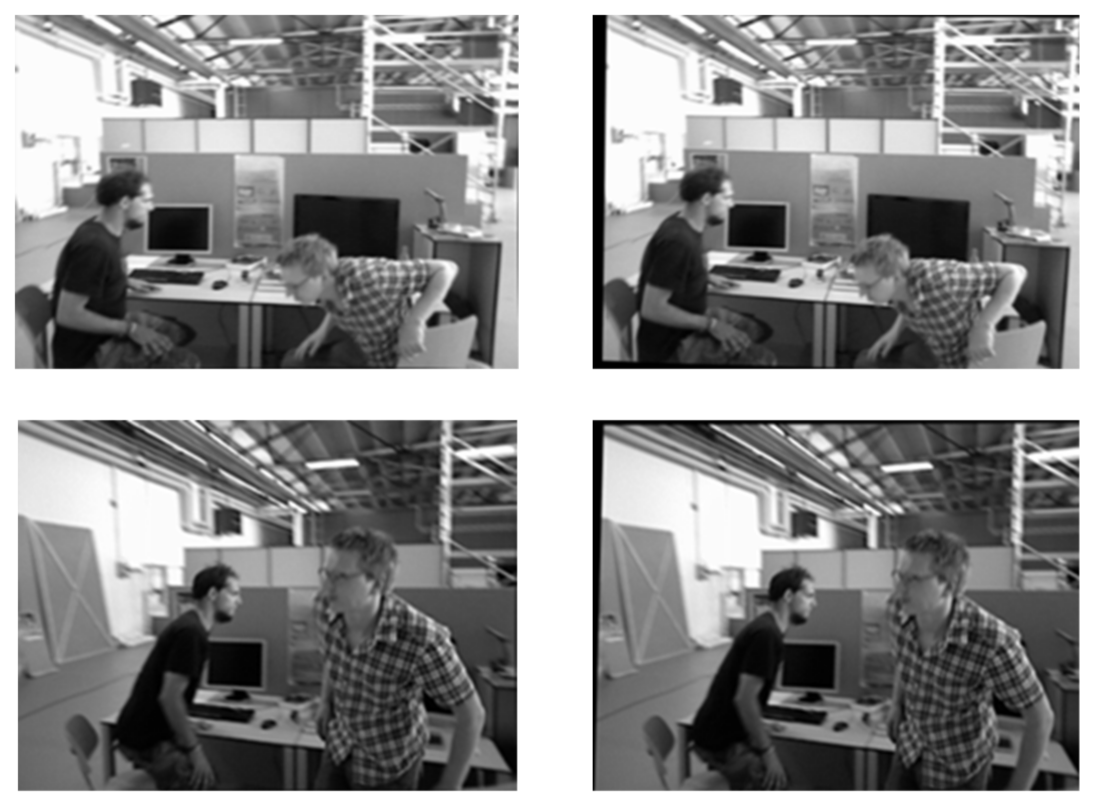
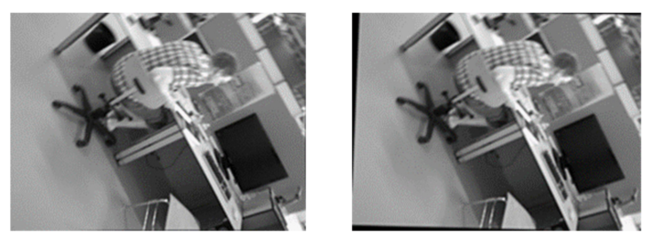
According to the homography transformation above, the motion component of an RGB-D camera itself within a current frame is compensated. A set of sample raw images and the compensation result of the motion component are shown in Figure 4. The black edge area of the rightmost column in Figure 4 represents the compensation of camera motion, while the leftmost are raw images.
Then the difference image is performed through the difference operation of adjacent image frames using (1):
where diffimg denotes the difference image, and and are adjacent image frames.
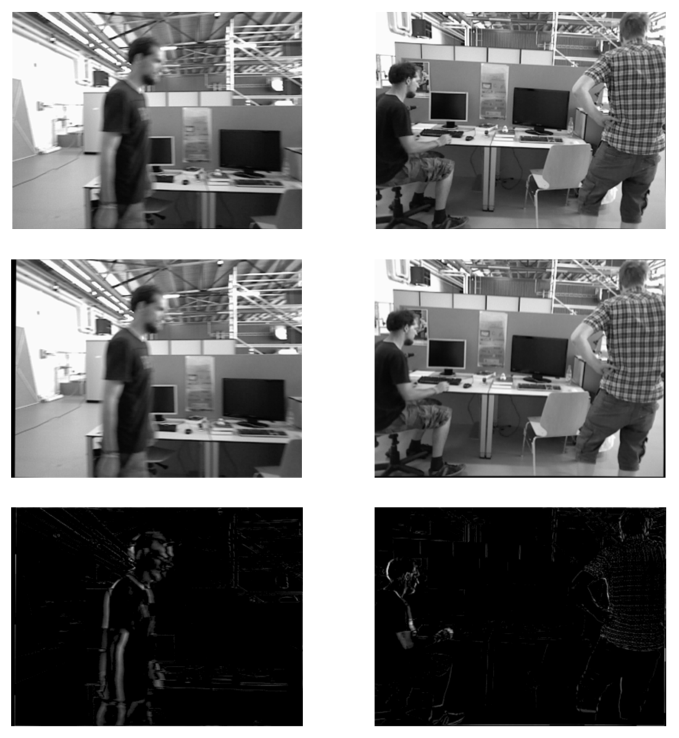
Figure 5 shows a group of sample raw images (Top row). and motion compensation images (Middle row) after applying the homography transformation, and the difference images (Bottom row) are acquired by performing the difference operation on the two frames. Since the background information of the scene shown in Figure 5 is static without any movement, the pixel values in the region of diffimg are 0. It is apparent and can be found in the bottom row of Figure 5. As the walking humans are in motion, the pixel values of the corresponding region on diffimg are not 0.
3.2. Dynamic Segmentation of the Depth Image Based on the Particle Filter
Assuming that represents the motion state of any particle point at any time of the particle filter, including the position and velocity of a particle, then, the state of particle point at the time is expressed using (2):
where and denote image coordinates of the ith particle point at the time t, and and are the corresponding velocity of particle point.
According to the basic principle of the particle filter, the posterior state estimation of the particle point is updated by an observation model and a motion model P(|), where the function P(|) represents the posterior conditional probability. In this section, is the particle point state information at the time t, and denotes a diffimg, which is calculated in Section 3.1 and regarded as an observation measurement. The observation model of can directly calculate the weight using pixel values from the diffimg and then consider it as the observation equation of the particle filter. The observation model here is used to evaluate the particle weight qualitatively. To make the calculation process more reasonable, the weight of each particle is decided by the Gaussian kernel function based on the observation measurement.
According to these pixels within the neighborhood of each particle, the way of calculating any particle’s importance weight, , is defined as:
where is the standard deviation of the Gaussian kernel function. d denotes the Euclidean distance between the particle point i and its neighborhood pixel , and the calculation formula of d is shown in Equation (4):
is a corresponding difference image obtained using (1), while I() represents the pixel value of the corresponding image point coordinates on the difference image. The motion model P(|) of particle filter can be expressed by a Gaussian distribution as:
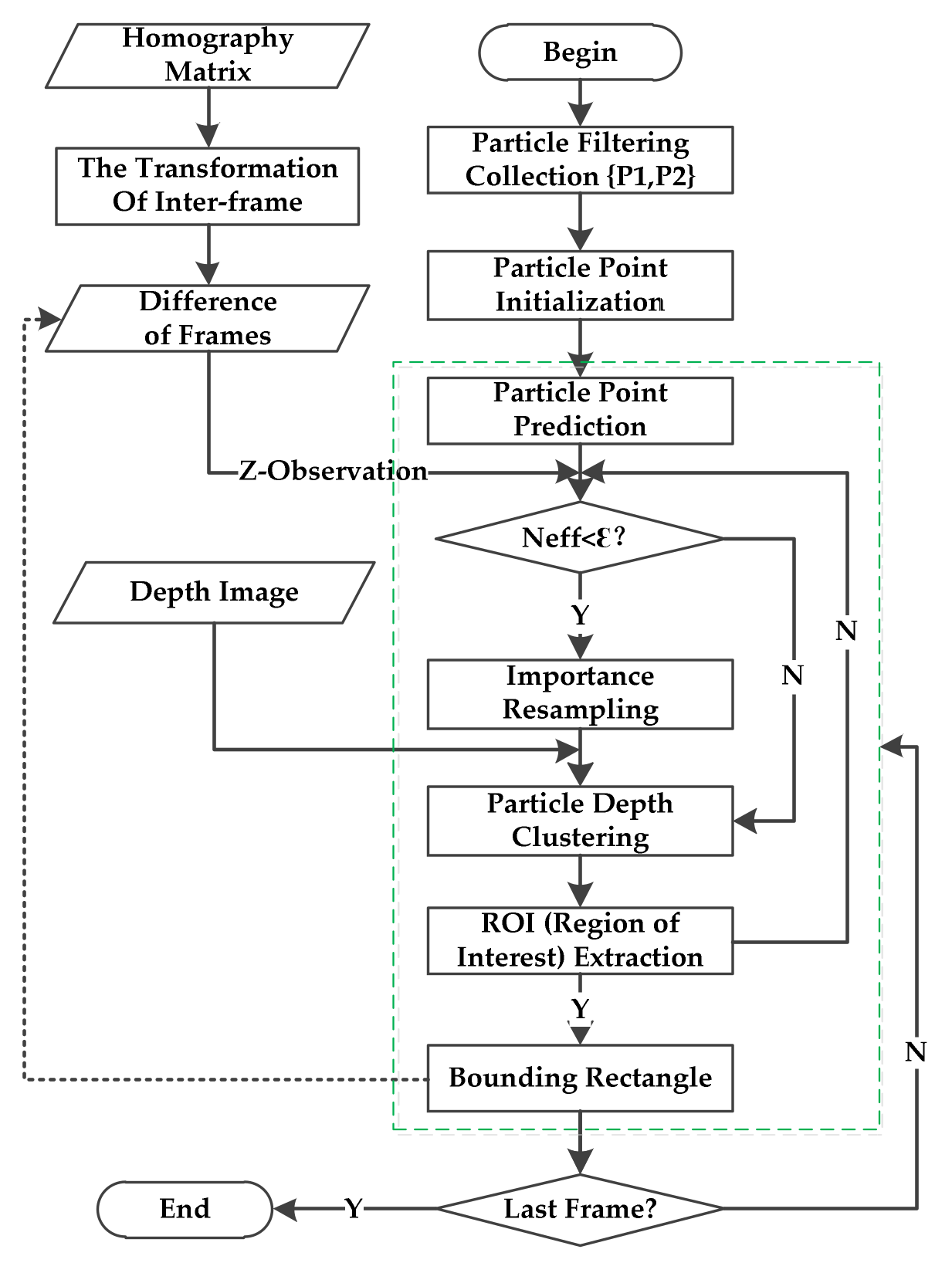
where and indicate the mean and variance of all previous particle points, and k represents the dimension of the particle state information. In the procedure of the particle filter, (5) is regarded as the state transition equation, which is used to predict the image coordinate position of each particle at the next moment. The flowchart of the dynamic segmentation algorithm based on the particle filter and depth image is given in Figure 6.
The specific steps of our proposed segmentation algorithm are as follows Algorithm 2:
| Algorithm 2: Dynamic segmentation based on the depth image and particle filter |
| Input: Difference Image Imgdiff, Depth image Imgdep, RGB image Imgrgb |
| Output: The bounding rectangle of dynamic region D |
| 0: Create a particle filter ; |
| 1: Initialize particle filter using the model of uniform distribution; |
| 2: Predicting particle position , using Equation (5); |
| 3: Update the weight using Imgdiff and Equation(3); |
| 4: Resampling. Performing resampling with the number of effective particles (Neff); |
| 5: Particles clustering. Clustering particles on Imgrgb and determining the ROI region; |
| 6: Depth clustering of particles. K-Means and Imgdep→particle depth clustering, deciding depth value interval (Udep) of particles; |
| 7: Segment region D using Udep, ROI, and Imgdep segment dynamic region D; |
| 8: Reprocess Imgdiff. Set pixel values of Imgdiff located in D to 0→new difference image Imgdiff2; |
| 9: After getting Imgdiff2, execute Step2~Step7 to search for another dynamic object; |
| 10: Judge if the current frame is the last one. If so, it is the end of the program; |
After tracking moving objects based on the particle filter, mass particles will gather and converge to the neighborhood of dynamic objects on the RGB images. It is difficult to describe the dynamic region on color images only depending on the particles. Inspired by [16], depth images are used to extract depth values and perform particle clustering with depth information. Firstly, the mean and variance of the particle state information are statistically estimated, and then, Gaussian distribution is applied to predict the pixel coordinates of particles at the next time. According to the pixel coordinates of convergent particles on RGB images and clustering results of those with depth images, there is a mass of particles in the neighborhood of dynamic objects. The depth intervals are determined using the statistical information of all particles belonging to the maximum clustering category. Then, the region of dynamic objects on a depth image can be segmented jointly based on the previously obtained depth interval and the predefining ROI (Region of Interest). Here, we set the height of the ROI as 640 pixels, and the width of the ROI could be fixed by the maximum and minimum coordinates of the clustered particles. After defining a binary image with the same size of 640 × 480 pixels, we traversed each pixel of ROI to judge whether its extraction depth is in the interval of depth value. If so, the pixel on the binary image is set to 1; otherwise, it is set to 0. After traversing all pixel elements of a depth image, the dynamic segmentation, a minimum bounding rectangle containing the motion object, will be gained by employing the function interface of OpenCV to find the maximum contour.
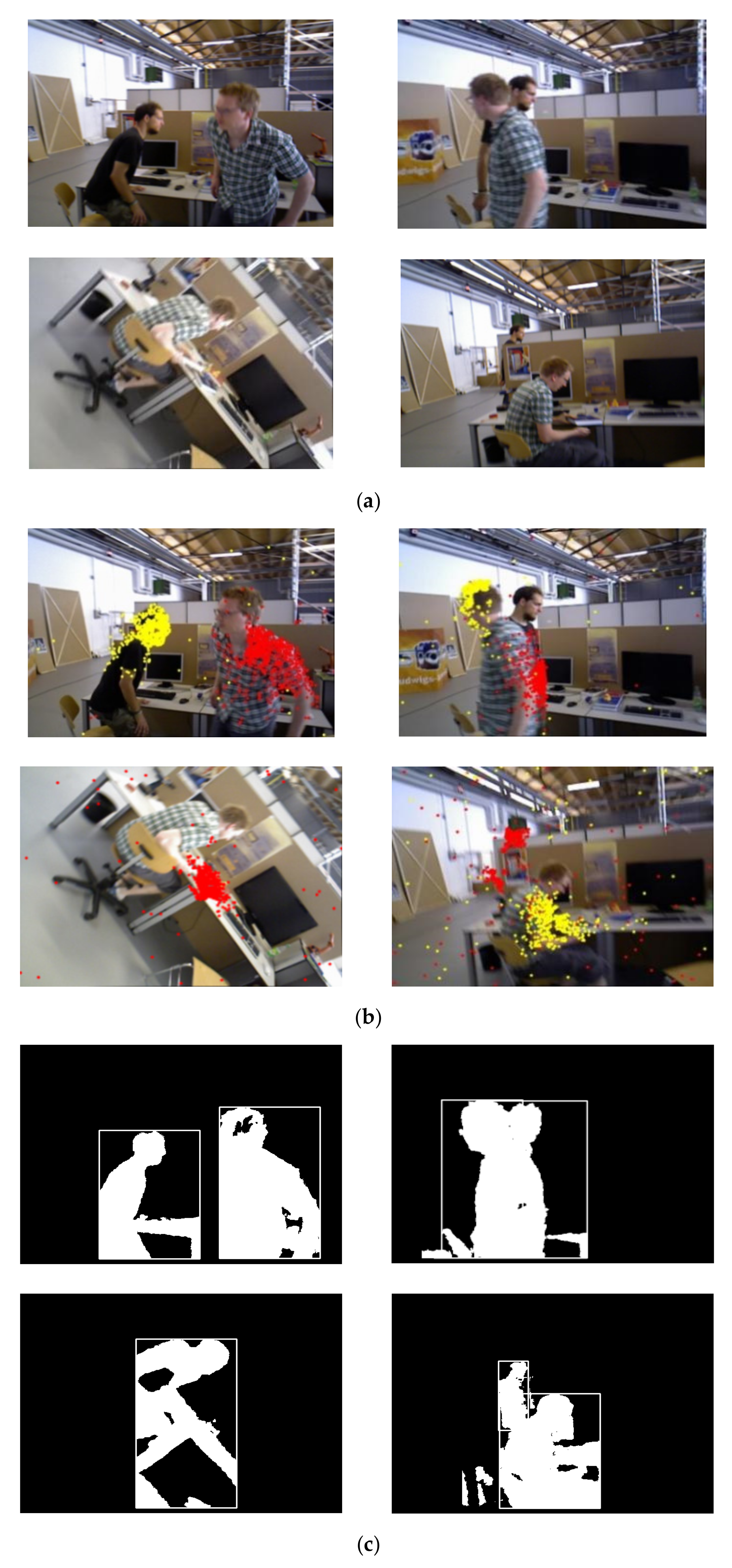
To demonstrate the effectiveness of our non-prior segmentation algorithm, we designed and selected several raw sample images of the public TUM datasets to test and verify. Figure 7 presents the segmentation and tracking results on the dynamic sequence named “fr3_walking_half_phere”, which provides 1067 frames and involves two persons walking through an indoor office scene. This sequence is captured by moving on a small half-sphere of approximately a one-meter diameter and can be used to evaluate the robustness of dynamic object segmentation. Figure 7a displays some raw color image examples, while Figure 7b,c show the related dynamic object segmentation and tracking effects. To visually display verification and experimental results, the yellow and red points denote the particle tracking results of two walking men separately. From the tracking results revealed in Figure 7b, mass particles gather around specific dynamic objectives dramatically. Subsequently, both the depth image and tracking result are adopted together to segment dynamic regions. It is concluded that our method can fulfill dynamic segmentation effectively according to the final responses presented in Figure 7c.
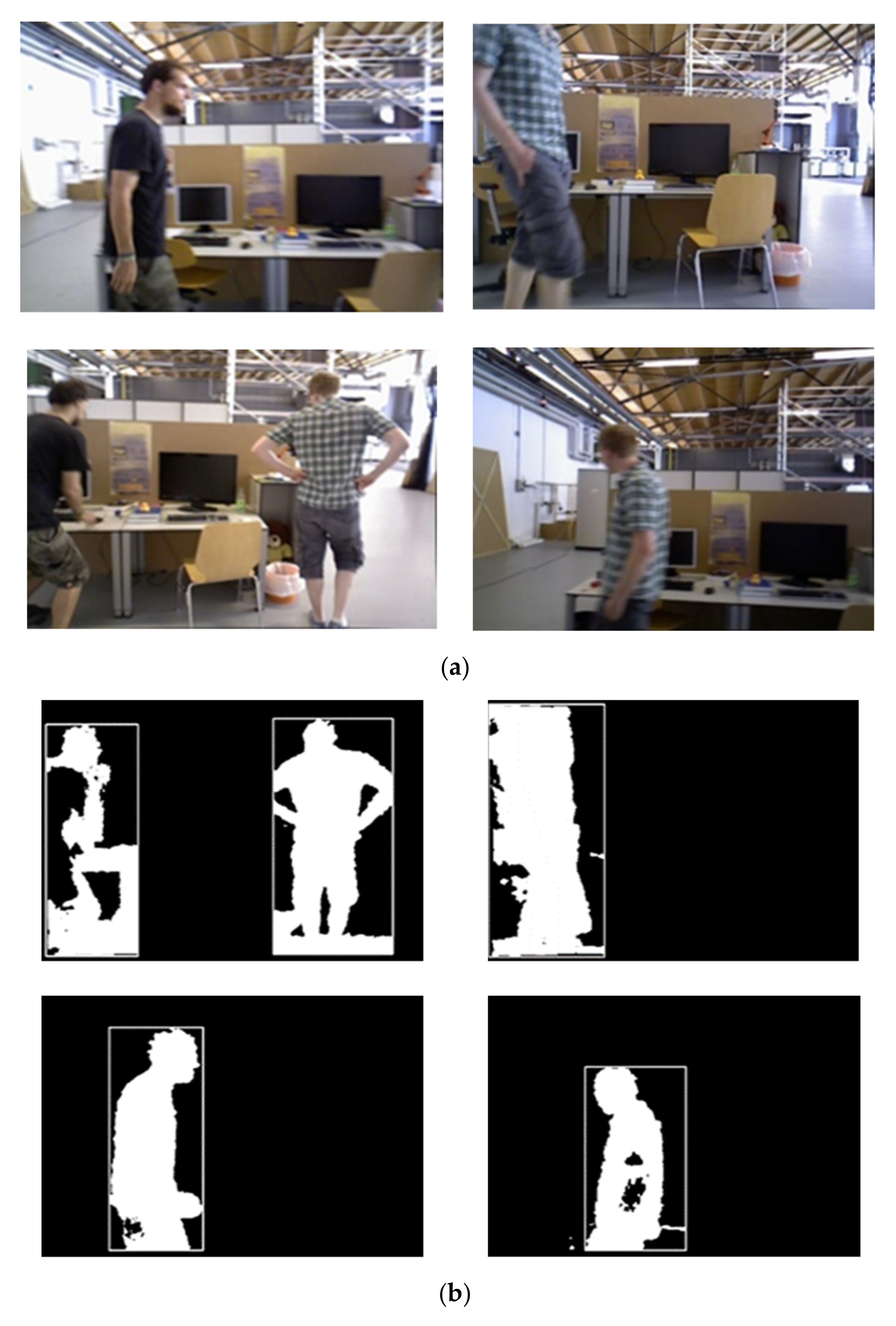
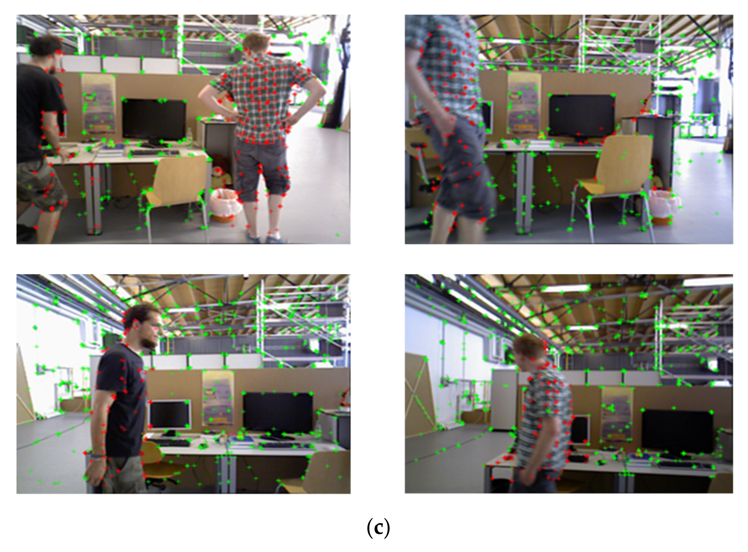
After segmenting these motion objects and obtaining dynamic regions, these dynamic point features are judged and rejected finely based on the K-Means algorithm. Please refer to the specific technical details in our previous work [37]. Figure 8 provides the static and dynamic point feature extraction results in the sequence of “fr3_walking_xyz”, which were acquired by moving the RGB-D camera along three directions (xyz) while keeping the same orientation. This sequence contains 827 frames and is intended to verify the effectiveness of object segmentation and visual SLAM algorithms in the dynamic scene. Figure 8a presents the raw RGB images, and Figure 8b gives the segmentation effects of dynamic objects. Figure 8c shows the feature extraction results of dynamic and static points, where the green + represents static point features, and the red + means that point features are dynamic.
4. Experimental Results
To verify the performance of PFD-SLAM based on our proposed non-prior information segmentation method, extensive experiments were conducted on the public TUM dynamic datasets and two real dynamic sequences. The TUM dataset is a well-known RGB-D benchmark to evaluate visual SLAM, whose dataset sequences were captured by an RGB-D camera. The image data were recorded in indoor dynamic scenes at a framerate of 30 Hz with a 640 × 480 pixel and provided the ground truth of camera trajectories captured by a motion-capture system with higher accuracy. As a result, major well-known dynamic SLAM algorithms have adopted the TUM datasets as their benchmark datasets. In these dynamic sequences (e.g., fr3_sitting: xyz, half_sphere, rpy, static; fr3_walking: xyz, half_sphere, rpy, static), “fr3_sitting” means that two persons sit at a desk, talk, and gesticulate a little, while “fr3_walking” denotes two persons walking through an office scene. All experiments were conducted on a laptop with an Intel®CoreTM 5-8250U@CPU of 1.6 GHz. The software utilized in our PFD-SLAM consists of the Linux operating system of Ubuntu 16.04, OpenCV 3.2.0, Eigen 3.0, and g2o.
Two evaluation indexes, ATE-RMSE (Root Mean Square Error, RMSE) of the absolute trajectory estimation (ATE) and RPE-RMSE (Relative Error of Pose Estimation), were for evaluating the overall accuracy and drift of camera trajectory. Given the estimation pose and the ground-truth , ATE-RMSE is calculated as follows:
where n is the number of frames in the data sequence. Assumin is the estimation pose, is the ground truth, and is a time interval. Given the total time N, RMSE-RPE is expressed as:
where m indicates the number of frames between the initial moment and the time N.
4.1. Dynamic Segmentation Particle Number Verification
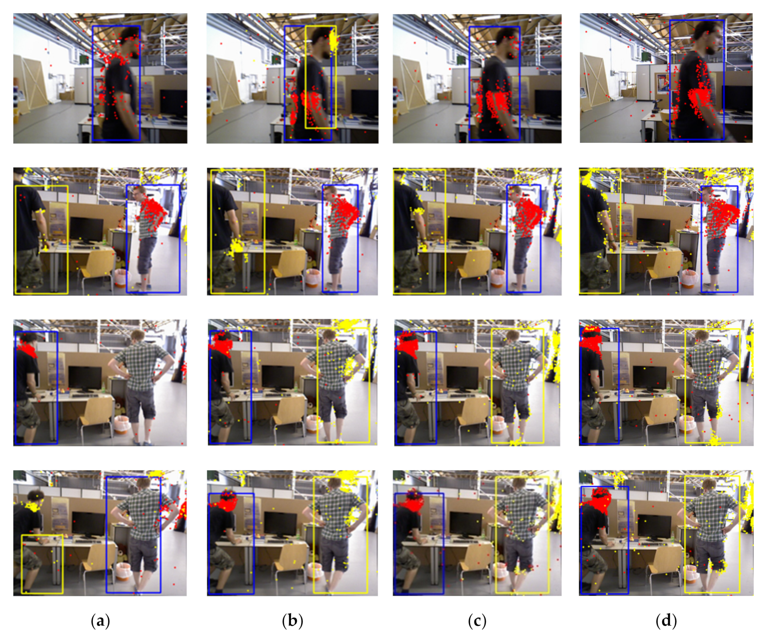
The qualitative and quantitative experiments were primarily conducted to search for the most suitable number of particles for dynamic object segmentation. Meanwhile, we offered the visual comparison result of motion object segmentation, and the absolute trajectory of camera estimation under the number of the particles were 500, 800, 1000, and 1200, quantitatively. Figure 9 shows the tracking and segmentation results of dynamic objects with different numbers of particles. The red and yellow points represent particles converging to different moving objects. In addition, the blue and yellow rectangles are the minimum bounding rectangles of motion objects.
From the dynamic object segmentation effects emerged in Figure 9, when the number of particles was 1000 or 1200, the overall segmentation results could achieve better robustness and accuracy. Meanwhile, when the number of particles was 1200, extra particle redundancy would occur, which is not beneficial to the overall dynamic segmentation. According to the obtained segmentation effects using 500 particles, the regions of dynamic objects on the RGB images were prone sub-segmentation or over-segmentation occurring. In the case of 800 particles, the segmentation accuracy of motion objects was improved significantly. Compared to the segmentation results based on 500 or 800 particles, the overall segmentation and tracking effect aiming at moving targets could be attained optimal with 1000 or 1200 particles.
The qualitative comparison experimental results are listed in Table 1, which contains the results of camera pose estimation in partial high and low dynamic scene sequences with different numbers of particles. Table 1 shows the ATE-RMSE and SD (Standard Deviation, S.D) of camera trajectories estimation on account of the segmentation effects. As the number of particles was 500, the accuracy and robustness of the camera pose estimation were the worst. However, in the case of 800 particles, the camera pose estimation accuracy was improved due to better segmentation effects of dynamic objects. Based on the qualitative comparison of ATE-RMSE under 1000 and 1200 particles, the accuracy of the camera pose could achieve the best performance in the case of optimal and robust segmentation effects. Through the qualitative and quantitative comparative analysis and the consideration of the running time of our algorithm, the number of particle points was selected as 1000 in the following experiments.
4.2. TUM Dynamic Dataset Experiments
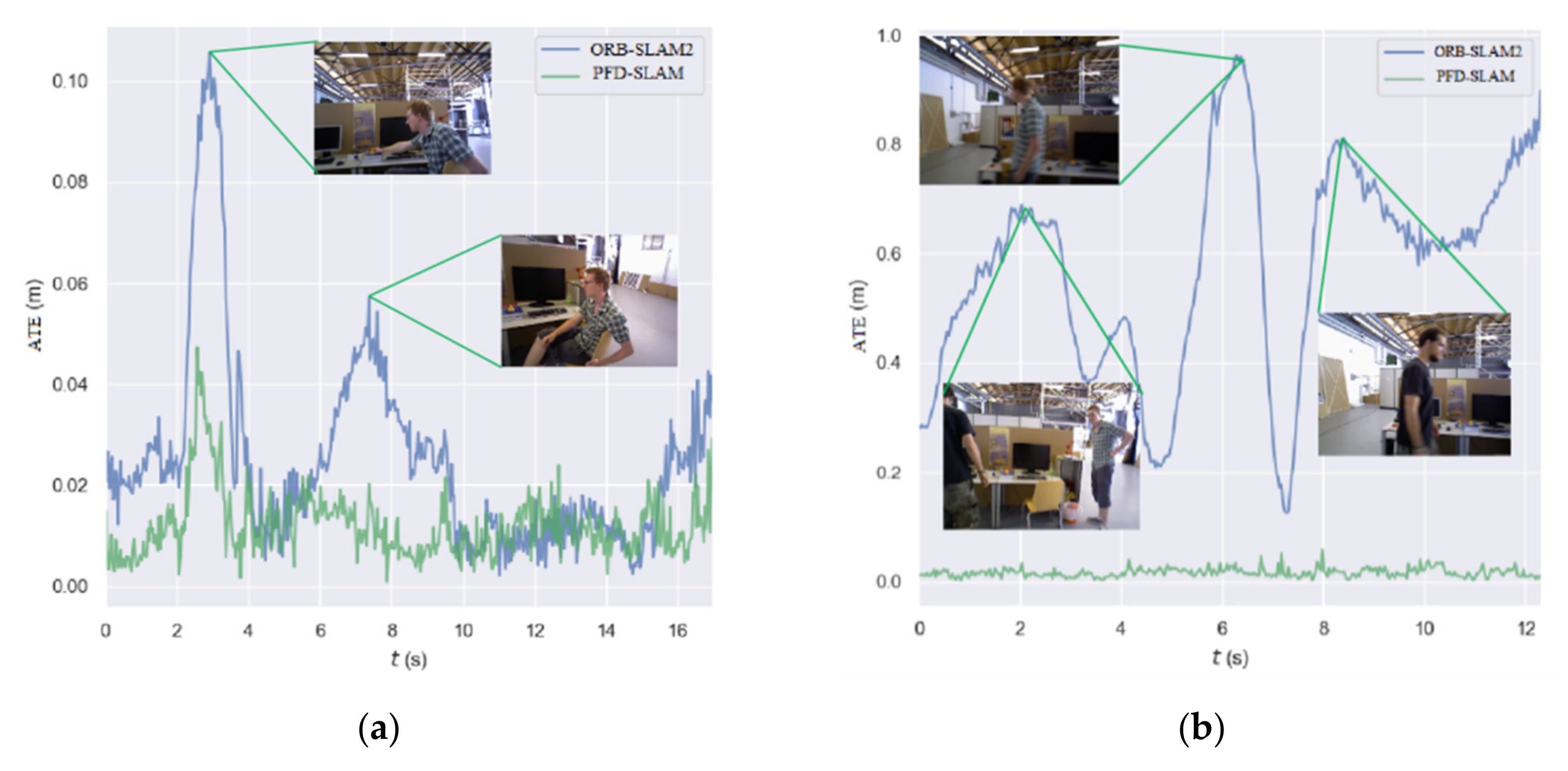
Firstly, we visualized the performance of PFD-SLAM and ORB-SLAM2 in two dynamic sequences. An open-source evaluation tool, Evo (Available online: https://github.com/MichaelGrupp/evo (accessed on 26 March 2022)), was utilized to plot the ATE distribution curves for the two dynamic sequences. As shown in Figure 10, the blue line represented the ATE of ORB-SLAM2, while the green line denoted the ATE of PFD-SLAM based on our proposed non-prior semantic segmentation model to segment dynamic objects. It can be seen from Figure 10 that when dynamic objects appeared in the indoor scenes, the ATE of ORB-SLAM2 increased dramatically. However, PFD-SLAM could significantly reduce the ATE at the exact moment by segmenting and removing the dynamic objects in the dynamic scenes.
Second, the experimental validation results on the publicly dynamic dataset were compared with several outstanding SLAM algorithms. Among these contrasting SLAM methods, MR-SLAM [16] was a motion removal method based on point features to handle the segmentation of dynamic elements. Still, it could track and segment one kind of dynamic object. Dyna-SLAM [25] adopted Mask-RCNN to segment semantic information and geometry constraints to deal with dynamic features. SPL-SLAM was a dynamic SLAM based on weights of static point-line components [38]. OPF-SLAM utilized the sparse optical flow to identify and reject these dynamic point features [20], while ORB-SLAM2 was a classic visual SLAM approach for static scenarios.
Table 2 summarizes these qualitative and quantitative experimental results of absolute camera trajectory error. “*” means that the algorithm did not provide the related experimental data, and the bold font indicates that the algorithm could achieve the best result of all comparison methods. “×” denotes that feature tracking failure occurred in the actual experiment. The experimental data in Table 2 were respectively from the results of the published paper and our actual test.
According to the experimental results given in Table 2, it is not difficult to find that PFD-SLAM could obtain the six best results from eight groups of experiments. In the “fr3_sitting_rpy” and “fr3_walking_static” sequences, even though PFD-SLAM could not complete the highest positioning accuracy, compared with five other SLAM methods, PFD-SLAM could also obtain the sub-optimal accuracy of camera absolute pose estimation. As MR-SLAM can segment one kind of dynamic object only and there is usually one more moving object in TUM dynamic sequences, the accuracy of camera absolute pose estimation is lower than that of other SLAM algorithms. As ORB-SLAM2 is unable to identify dynamic point features, its camera pose accuracy is the weakest of all comparison SLAM algorithms. OPF-SLAM applied optical flow to detect and eliminate dynamic features, but its robustness is weaker in the high dynamic sequences. SPL-SLAM calculates the camera pose based on the static weights of point-line visual elements, which is only based on image feature-level segmentation. Dyna-SLAM outperformed PFD-SLAM on the “fr3_walking_half” and “fr3_walking_rpy”, but it should be noted that Dyna-SLAM was based on deep learning with an accurate semantic segmentation effect. The potential advantage of PFD-SLAM was that it did not rely on deep learning and could obtain comparable positioning accuracy. In addition, due to the complex motion styles of dynamic objects in the scene and the influence of camera rotation and image blur, when the static or dynamic components are recognized by depending on the weights in high dynamic sequence, SPL-SLAM is prone to misclassifying individual dynamic features as static, which reduces the optimization accuracy of the camera pose.
The translational drift and the relative pose rotation drift are mainly used to measure the part drift of visual odometry in the front of the whole SLAM system. The relative errors of pose translation and the pose of SLAM methods above in the TUM dynamic dataset are listed in Table 3 and Table 4, where the bold font still indicates the best result of the RPE-RMSE. According to the comparison results given in Table 3 and Table 4, as PFD-SLAM could segment dynamic objects and eliminate dynamic features on these low or high dynamic scene sequences well, PFD-SLAM owned significant advantages over the contrasting SLAM methods in reducing rotation and poses errors.
To compare the overall visual camera motion trajectory error intuitively, Figure 10 offers the error comparison results of camera estimation trajectories and ground truth. Our proposed PFD-SLAM was comprehensively compared with ORB-SLAM2, OPF-SLAM, and Dyna-SLAM. In Figure 11 and Figure 12, the black lines are the ground truth of camera trajectories, while the blue lines denote the estimated trajectories. Moreover, the red lines show the absolute difference between the estimated trajectories and the ground truth, and the yellow rectangle box indicates that the method had tracking loss in some frames.
Figure 11 shows the difference between the estimation trajectories and ground truth on the high dynamic sequence. As Dyna-SLAM has an inherent advantage of an accurate semantic segmentation, it could accomplish the experiments and showed stronger robustness. Although the visual comparison of PFD-SLAM and Dyna-SLAM were a little different, the overall positioning accuracy of PFD-SLAM was still relatively higher, as seen in Table 2. Compared with OPF-SLAM and ORB-SLAM2 comprehensively, as our proposed PFD-SLAM could segment dynamic objects and recognized the dynamic features efficiently, it could achieve higher accuracy and robustness of pose estimation.
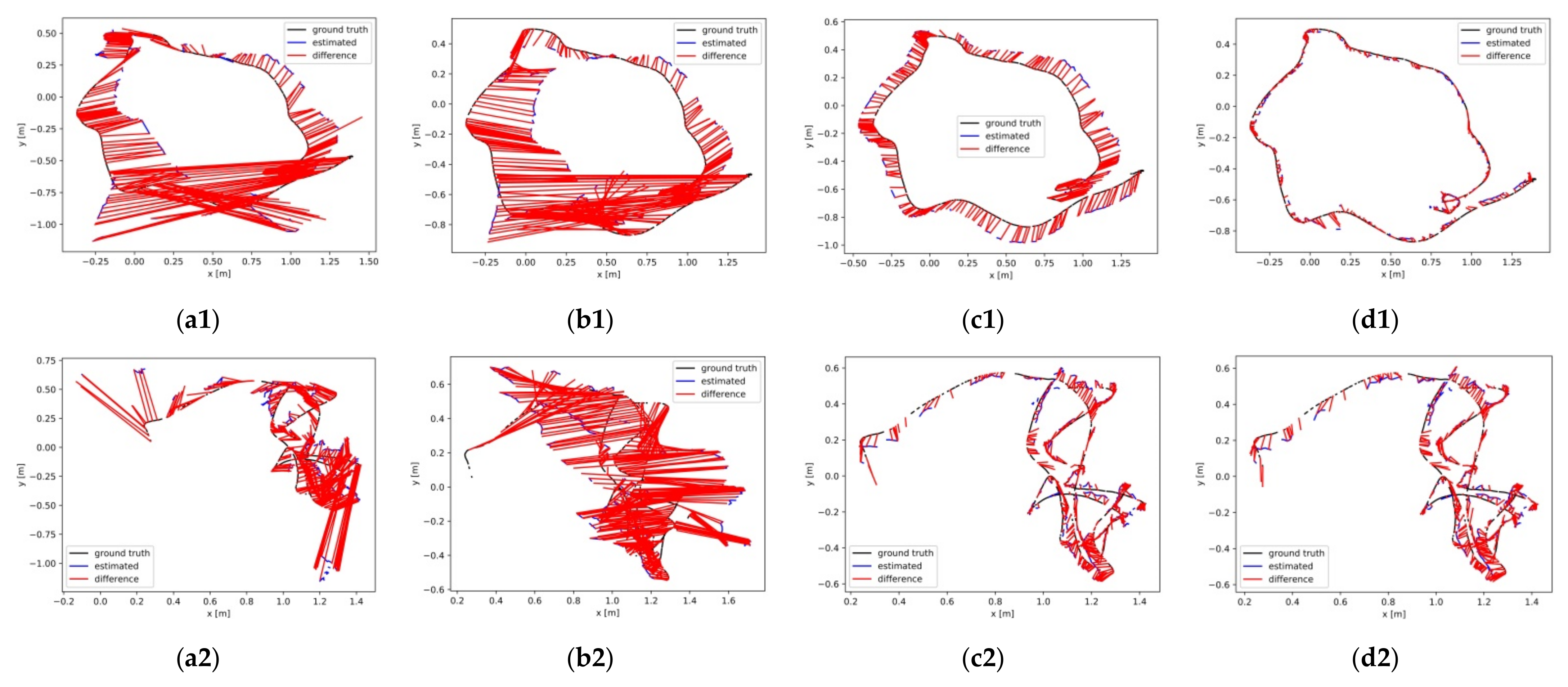
Figure 12 shows the differences between the camera estimation trajectories and ground truth on three groups of dynamic sequences (“fr3_s_static, fr3_s_xyz, fr3_s_half”). According to the intuitive comparisons, the features tracking loss occurred in Dyna-SLAM. Although all four algorithms could accomplish the experiments, PFD-SLAM could achieve the lowest camera pose estimation error of all.
4.3. Real Scene
To verify the effectiveness of PFD-SLAM in real scenes, the dynamic scene dataset provided by Cheng [12] was utilized for testing practical performances in real scenes. ORB-SLAM2, OPF-SLAM, Dyna-SLAM, and PFD-SLAM were all conducted in two groups of experiments on two real dynamic scene sequences. The dynamic sequences were captured at a framerate of 30 Hz with an Asus Xtion RGB-D sensor in the real scene. In addition to the dynamic objects, the dataset also included fast motion and blurred images, which was a challenging dynamic data sequence. The corresponding ground truth of camera trajectories was recorded by a motion-capture system, which was used to evaluate the practical performance.
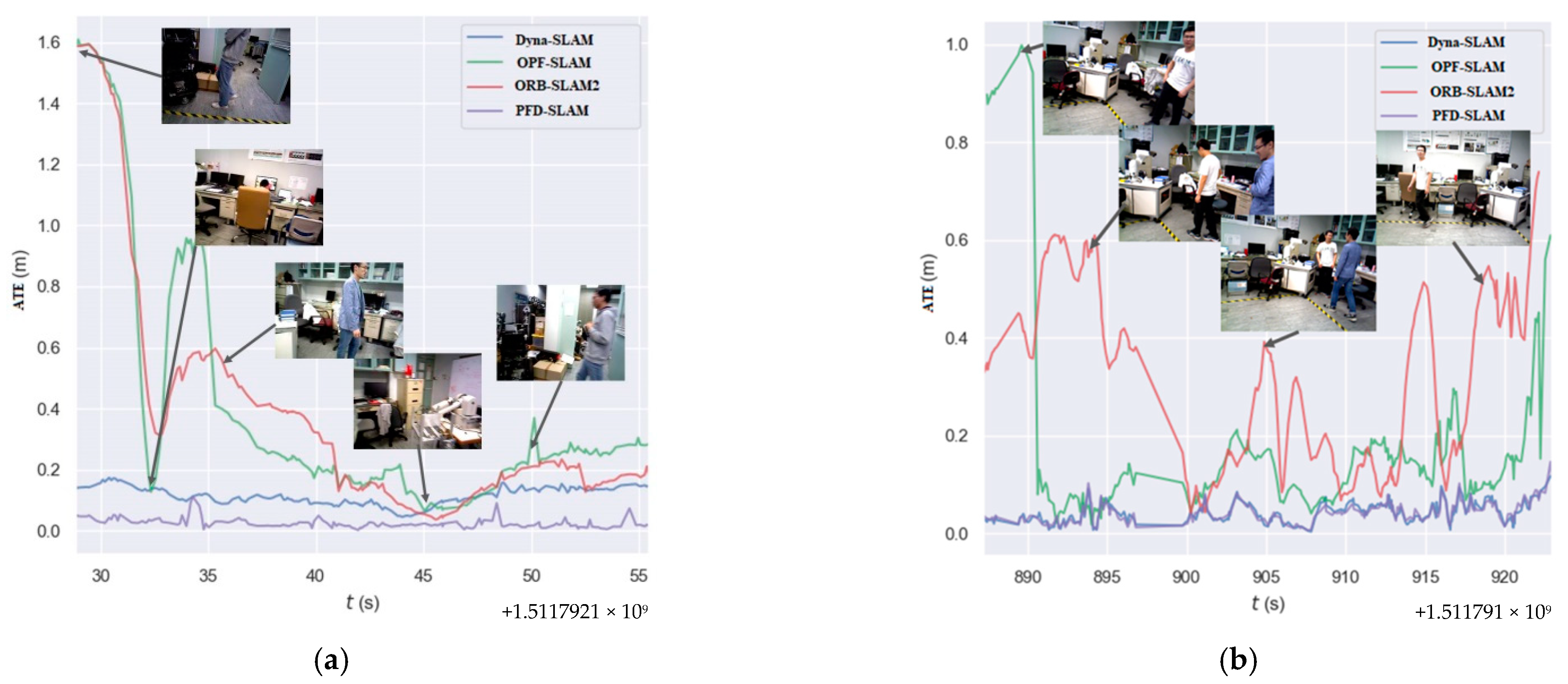
Firstly, we also visualized the contrast results of PFD-SLAM, ORB-SLAM2, OPF- SLAM, and Dyna-SLAM in two dynamic sequences. The distribution curves of ATE are shown in Figure 13. It can be seen from Figure 13 that PFD-SLAM could significantly reduce the ATE by segmenting and removing dynamic objects in the dynamic scenes.
Here, the ATE-RMSE, RPE-RMSE, and S.D describing the stability indicator of visual SLAM all were taken as the evaluation indexes. The absolute pose estimation errors of three algorithms in dynamic scenes are given in Table 5, and the bold fonts still indicate the best result of all three approaches. According to the experimental comparison results presented in Table 5, the absolute camera pose estimation accuracy obtained by PFD-SLAM in real dynamic scenes was superior to that of ORB-SLAM2, OPF-SLAM, and Dyna-SLAM.
The results of the camera relative pose estimation error and relative rotation error of the above three algorithms are shown in Table 6 and Table 7. According to the comparison results presented in Table 6 and Table 7, the relative accuracy of PFD-SLAM in the real dynamic scene was higher than that of ORB-SLAM2 and OPF-SLAM. According to these comparison experimental results of standard deviation, PFD-SLAM still could reveal stronger robustness than ORB-SLAM2 and OPF-SLAM.
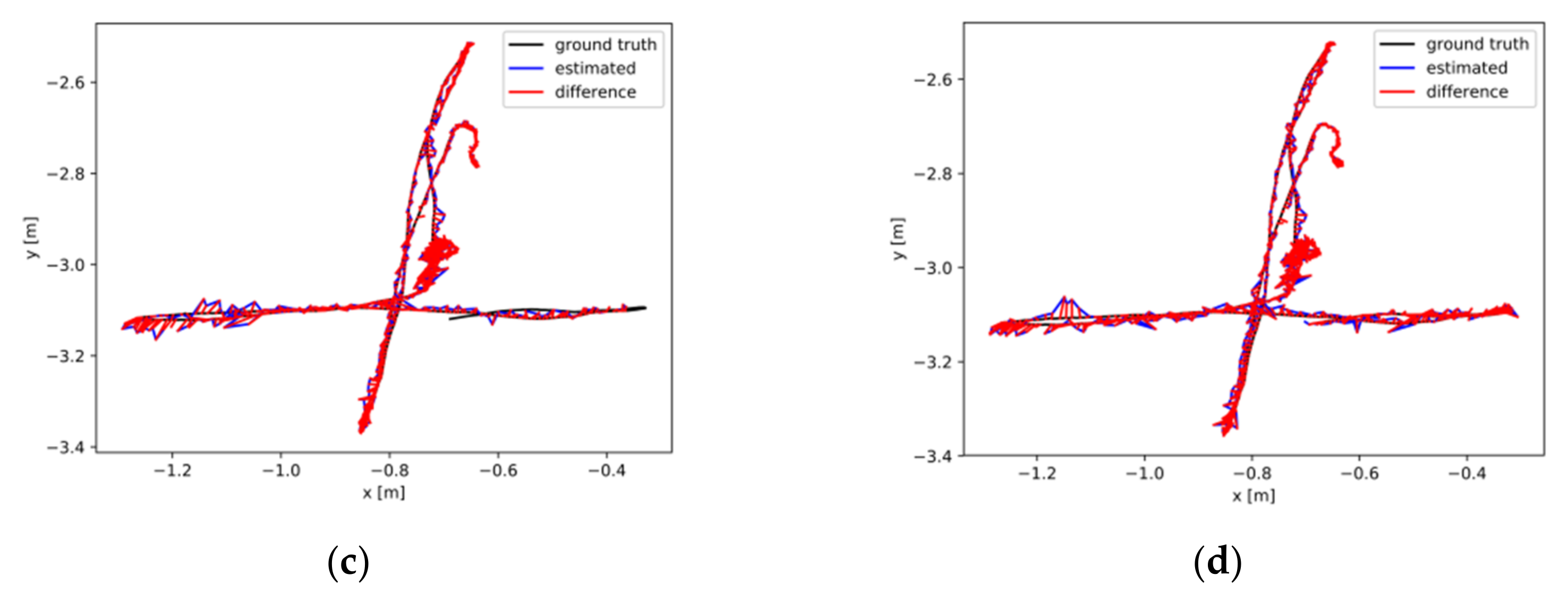
The camera estimation trajectories of the above three algorithms in two groups of real dynamic scenes were also compared visually. Figure 14 shows the difference between the camera estimation trajectories and the corresponding ground truth. In light of these comparison results visually displayed in Figure 14, compared with OPF-SLAM, ORB-SLAM2, and Dyna-SLAM, PFD-SLAM performed more accurate camera pose estimation results and showed stronger stability.
4.4. Running Time Analysis
The efficiency is an essential indicator for visual SLAM, and we investigated the efficiency performance of PFD-SLAM. To evaluate the PDF-SLAM running efficiency, we counted the average running time consumption of the different modules. The experiments were conducted on our laptop computer equipped with general configuration parameters of the CPU. Table 8 summarizes the average running times of several parts of PFD-SLAM tested on the TUM and real scene datasets. The average running time of PFD-SLAM processing each frame fluctuated between 0.1 and 0.12 s, which met the real-time operation generally.
Because our non-prior semantic segmentation strategy involved the calculator of the difference images and extensive array traversal operations, it made our segmentation method consume more computing time. The tracking based on particle filter and the identification and segmentation of motion objects were the most time-consuming. Furthermore, as PFD-SLAM was executed on an inefficient CPU and the original raw images were not compressed before input, it needed to consume a little more time. Due to this limitation of PFD-SLAM, the efficiency of PFD-SLAM will be improved in our future work. There is another feasible solution to address this problem in the future. An efficient approach is to deploy a server with a higher hardware configuration to accelerate the running speed of SLAM. Another way is to improve our segmentation algorithm program and optimize the execution process of the current program with multi-threaded programming technology.
5. Discussion
In the experimental results of Table 2, Table 3 and Table 4, PFD-SLAM and these contrasting dynamic SLAMs all finished the validation experiments. In comparison to the ATE-RMSE and RPE-RMSE results of classical SLAM [17,20,25,38], PFD-SLAM achieved 5–6 improvements in the public TUM datasets. The reference dynamic SLAM methods (e.g., MR-SLAM, SPL-SLAM, OPF-SLAM) are based on mathematical models to eliminate outlier features, and they easily have sub-segmentation or over-segmentation of features arise. The inaccurate segmentation of dynamic features usually causes several wrong data associations, which degenerate the accuracy and robustness of camera pose estimation to some extent. For instance, as MR-SLAM can segment one kind of motion object merely when there is one more dynamic object, it cannot obtain more accurate pose estimation results normally. As the motions of the camera and dynamic object are relatively complex, OPF-SLAM based on optical flow cannot detect dynamic features effectively. Therefore, it cannot acquire satisfactory performances or even have tracking loss occur in the sequence of “fr3_walking_rpy”. This is because ORB-SLAM2 is not able to discern static and dynamic features accurately. For low dynamic sequences with little effect on camera pose estimation, it can achieve comparable accuracy in four low dynamic sequences (e.g., fr3_sitting_static, fr3_sitting_rpy).
Nevertheless, in high dynamic scenes, ORB-SLAM2 could not perform powerful performances generally. Dyna-SLAM adopted prior semantic information to determine dynamic features, and PFD-SLAM based on non-prior semantic object segmentation outperformed performance in most sequences. For the verification of real settings, we also designed and executed some comparison experiments. The experimental results are displayed in Figure 11 and Figure 12 and Table 2, Table 3 and Table 4, and PFD-SLAM still achieved better performances than ORB-SLAM2 and OPF-SLAM.
However, as the segmentation accuracy of our segmentation model was dependent on the posterior estimation model of the particle filter, some extra factors, including the complexity of moving objects, vibration, rotation within cameras, and blurred images, would interfere closely with the transformation of adjacent frames. This transformation, an observation measurement of particle filter, would affect the segmentation accuracy and influence the location accuracy of the camera finally. For instance, for the sequences with rotation and blur images (e.g., fr3_sitting_rpy, fr3_walking_rpy), PFD-SLAM could perform a mildly moderate performance, and improvement work will be done in the feature.
It can be concluded from the experimental results of Table 2, Table 3, Table 4, Table 5, Table 6 and Table 7 and Figure 9, Figure 10, Figure 11, Figure 12, Figure 13 and Figure 14 as follows: PFD-SLAM utilizes the particle filter to segment dynamic objects, and it is also different from most dynamic SLAM methods, which are based on mathematical models to achieve the feature-level segmentation only. As PFD-SLAM can attain object-level segmentation, it can obtain more remarkable improvements than other dynamic SLAM schemes (MR-SLAM, SPL-SLAM). Compared to these performances of ORB- SLAM2 and OPF-SLAM in low dynamic sequences, although PFD-SLAM performed some slight improvements in location accuracy, it also achieved better or comparable performances. Finally, according to the experimental results discussed above, it was demonstrated that the dynamic segmentation based on non-prior information within PFD-SLAM possesses a certain generalization of motion segmentation and practical application potentiality aiming at dynamic scenes.
6. Conclusions
In this paper, we presented a new dynamic object segmentation method based on non-prior semantic information. Then, we fused the motion region segmentation into the front end of SLAM and established PFD-SLAM for dynamic scenes. To obtain more accurate and robust segmentation results, we combined GMS and sparse optical flow to calculate the inter-frame transformation, firstly, a prerequisite for dynamic segmentation based on a particle filter. Next, the difference image was calculated and regarded as an observation measurement of the particle filter, while Gaussian distribution was considered as a motion equation of the filter. After establishing the motion and observation equation, both the depth image and RGB image were utilized to implement the dynamic object segmentation. After finishing the segmentation steps, we fused the segmentation model into the front end of SLAM to reduce the influence of dynamic objects and wrong data association in dynamic scenes. Extensive experimental results have proved that PFD-SLAM can improve the accuracy and robustness of pose calculation in dynamic scenes. We compared PFD-SLAM with some outstanding dynamic SLAMs. It was also demonstrated that PFD-SLAM can perform apparent improvements in dynamic sequences. PFD-SLAM showed a few poor performances on extra dynamic scene sequences, but it achieved comparable accuracy and performances too.
However, despite the excellent performance, PFD-SLAM also requires some ongoing work. For instance, rapid rotation within a camera and the blur images usually make the segmentation method restrict, which limits camera pose estimation accuracy. In the future, we will integrate the IMU (Inertial Measurement Unit) into PFD-SLAM. The pose information provided by the IMU will help overcome the wrong segmentation caused by rapid rotation of a camera or blurred images and extra factors in the dynamic settings.
Author Contributions
C.Z. conceived the idea and methods; C.Z. and S.J. performed experiments and validation; R.Z. analyzed the data; C.Z., R.Z., S.J. and X.Y. wrote and revised the paper. All authors have read and agreed to the published version of the manuscript.
Funding
This research was funded by the National Natural Science Foundation of China (41901401), the Natural Science Foundation of Jiangsu Province (BK20190743), and the China Postdoctoral Science Foundation (2021M691653).
Data Availability Statement
Publicly available datasets were analyzed in this study. This data can be found here: http://vision.in.tum.de/data/datasets/rgbd-dataset (accessed on 5 April 2022).
Acknowledgments
We thank the Computer Vision Group from the Technical University of Munich and Imperial College London and National University for making the RGB-D SLAM datasets publicly available. We also thank Qiang Fu from the National Engineering Laboratory for Robot Visual Perception and Control Technology, Hunan University, for his help on this research.
Conflicts of Interest
The authors declare no conflict of interest.
References
- Di, K.; Wan, W.; Zhao, H.; Liu, Z.; Wang, R.; Zhang, F. Progress and Applications of Visual SLAM. Acta Geod. Cartogr. Sin. 2018, 47, 770–779. [Google Scholar]
- Qingquan, L.I.; Baoding, Z.H.; Wei, M.A.; Weixing, X.U. Research process of GIS-aided indoor localization. Acta Geod. Cartogr. Sin. 2019, 48, 1498–1506. [Google Scholar]
- Fu, Q.; Yu, H.; Wang, X.; Yang, Z.; He, Y.; Zhang, H.; Mian, A. Fast ORB-SLAM Without Keypoint Descriptors. IEEE Trans. Image Process. 2022, 31, 1433–1446. [Google Scholar] [CrossRef] [PubMed]
- Hong, S.; Bangunharcana, A.; Park, J.M.; Choi, M.; Shin, H.S. Visual SLAM-Based Robotic Mapping Method for Planetary Construction. Sensors 2021, 21, 7715. [Google Scholar] [CrossRef] [PubMed]
- Piao, J.C.; Kim, S.D. Real-Time Visual–Inertial SLAM Based on Adaptive Keyframe Selection for Mobile AR Applications. IEEE Trans. Multimed. 2019, 21, 2827–2836. [Google Scholar] [CrossRef]
- Bresson, G.; Alsayed, Z.; Yu, L.; Glaser, S. Simultaneous Localization and Mapping: A Survey of Current Trends in Autonomous Driving. IEEE Trans. Intell. Veh. 2017, 2, 194–220. [Google Scholar] [CrossRef] [Green Version]
- Mur-Artal, R.; Tardós, J.D. ORB-SLAM2: An Open Source SLAM System for Monocular, Stereo, and RGB-D Cameras. IEEE Trans. Robot. 2017, 33, 1255–1262. [Google Scholar] [CrossRef] [Green Version]
- Kerl, C.; Sturm, J.; Cremers, D. Dense visual SLAM for RGB-D Cameras. In Proceedings of the 2013 IEEE/RSJ International Conference on Intelligent Robots and Systems, Tokyo, Japan, 3–7 November 2013; pp. 2100–2106. [Google Scholar]
- Qin, T.; Li, P.; Shen, S. VINS-Mono: A Robust and Versatile Monocular Visual-Inertial State Estimator. IEEE Trans. Robot. 2018, 34, 1004–1020. [Google Scholar] [CrossRef] [Green Version]
- Bian, J.; Lin, W.Y.; Matsushita, Y.; Yeung, S.K.; Nguyen, T.D.; Cheng, M.M. Gms: Grid-based motion statistics for fast, ultra-robust feature correspondence. In Proceedings of the IEEE Conference on Computer Vision and Pattern Recognition (CVPR), Honolulu, HI, USA, 21–26 July 2017; pp. 4181–4190. [Google Scholar]
- Sturm, J.; Engelhard, N.; Endres, F.; Burgard, W.; Cremers, D. A benchmark for the evaluation of RGB-D SLAM systems. In Proceedings of the 2012 IEEE/RSJ International Conference on Intelligent Robots and Systems, Vilamoura-Algarve, Portugal, 7–12 October 2012; pp. 573–580. [Google Scholar]
- Cheng, J.; Zhang, H.; Meng, M.Q. Improving Visual Localization Accuracy in Dynamic Environments Based on Dynamic Region Removal. IEEE Trans. Autom. Sci. Eng. 2020, 17, 1585–1596. [Google Scholar] [CrossRef]
- Gao, X.; Shi, X.; Ge, Q.; Chen, K. A Survey of Visual SLAM for Scenes with Dynamic Objects. Robot 2021, 43, 733–750. [Google Scholar]
- Wang, C.C.; Thorpe, C. Simultaneous localization and mapping with detection and tracking of moving objects. In Proceedings of the 2002 IEEE International Conference on Robotics and Automation (Cat. No.02CH37292), Washington, DC, USA, 11–15 May 2002; pp. 2918–2924. [Google Scholar]
- Wang, Y.; Huang, S. Towards dense moving object segmentation based robust dense RGB-D SLAM in dynamic scenarios. In Proceedings of the 2014 13th International Conference on Control Automation Robotics& Vision (ICARCV), Singapore, 10–12 December 2014; pp. 1841–1846. [Google Scholar]
- Bakkay, M.C.; Arafa, M.; Zagrouba, E. Dense 3D SLAM in dynamic scenes using Kinect. In Proceedings of the 7th Iberian Conference on Pattern Recognition and Image Analysis, Santiago de Compostela, Spain, 17–19 June 2015; pp. 121–129. [Google Scholar]
- Sun, Y.; Liu, M.; Meng, Q.H. Improving RGB-D SLAM in dynamic environments: A motion removal approach. Robot. Autom. Syst. 2017, 89, 110–122. [Google Scholar] [CrossRef]
- Kim, D.H.; Kim, J.H. Effective Background Model-Based RGB-D Dense Visual Odometry in a Dynamic Environment. IEEE Trans. Robot. 2017, 32, 1565–1573. [Google Scholar] [CrossRef]
- Wang, R.; Wan, W.; Wang, Y.; Di, K. A New RGB-D SLAM Method with Moving Object Detection for Dynamic Indoor Scenes. Remote Sens. 2019, 11, 1143. [Google Scholar] [CrossRef] [Green Version]
- Cheng, J.; Sun, Y.; Meng, M.Q. Improving monocular visual SLAM in dynamic environments: An optical-flow-based approach. Adv. Robot. 2019, 33, 576–589. [Google Scholar] [CrossRef]
- Alcantarilla, P.F.; Yebes, J.J.; Almazán, J.; Bergasa, L.M. On combining visual SLAM and dense scene flow to increase the robustness of localization and mapping in dynamic environments. In Proceedings of the 2012 IEEE International Conference on Robotics and Automation (ICRA), Saint Paul, MN, USA, 14–18 May 2012; pp. 1290–1297. [Google Scholar]
- Zou, D.; Tan, P. CoSLAM: Collaborative visual SLAM in dynamic environments. IEEE. Trans. Pattern Anal. Mach. Intell. 2013, 35, 354–366. [Google Scholar] [CrossRef]
- Liu, G.; Zeng, W.; Feng, B.; Xu, F. DMS-SLAM: A General Visual SLAM System for Dynamic Scenes with Multiple Sensors. Sensors 2019, 19, 3714. [Google Scholar] [CrossRef] [Green Version]
- Kim, D.H.; Han, S.B.; Kim, J.H. Visual odometry algorithm using an RGB-D sensor and IMU in a highly dynamic environment. In Robot Intelligence Technology and Applications 3; Springer: Cham, Switzerland, 2015; pp. 11–26. [Google Scholar]
- Bescos, B.; Fácil, J.M.; Civera, J.; Neira, J. DynaSLAM: Tracking, mapping, and in painting in dynamic scenes. IEEE Robot. Autom. Lett. 2018, 3, 4076–4083. [Google Scholar] [CrossRef] [Green Version]
- He, K.; Gkioxari, G.; Dollár, P.; Girshick, R. Mask R-CNN. IEEE Trans. Pattern Anal. Mach. Intell. 2020, 42, 386–397. [Google Scholar] [CrossRef]
- Zhang, Z.; Zhang, J.; Tang, Q. Mask R-CNN Based Semantic RGB-D SLAM for Dynamic Scenes. In Proceedings of the 2019 IEEE/ASME International Conference on Advanced Intelligent Mechatronics (AIM), Hong Kong, China, 8–12 July 2019; pp. 1151–1156. [Google Scholar]
- Yu, C.; Liu, Z.; Liu, X.J.; Xie, F.; Yang, Y.; Wei, Q.; Fei, Q. Ds-slam: A semantic visual slam towards dynamic environments. In Proceedings of the IEEE/RSJ International Conference on Intelligent Robots and Systems (IROS), Madrid, Spain, 1–5 October 2018; pp. 1168–1174. [Google Scholar]
- Cui, L.; Ma, C. SOF-SLAM: A Semantic Visual SLAM for Dynamic Environments. IEEE Access 2019, 7, 166528–166539. [Google Scholar] [CrossRef]
- Han, S.; Xi, Z. Dynamic Scene Semantics SLAM Based on Semantic Segmentation. IEEE Access 2020, 8, 43563–43570. [Google Scholar] [CrossRef]
- Yuan, X.; Chen, S. SaD-SLAM: A Visual SLAM Based on Semantic and Depth Information. In Proceedings of the 2020 IEEE/RSJ International Conference on Intelligent Robots and Systems (IROS), Las Vegas, NV, USA, 24 October 2020–24 January 2021; pp. 4930–4935. [Google Scholar]
- Cui, L.; Ma, C. SDF-SLAM: Semantic Depth Filter SLAM for Dynamic Environments. IEEE Access 2020, 8, 95301–95311. [Google Scholar] [CrossRef]
- Ran, T.; Yuan, L.; Zhang, J.; Tang, D.; He, L. RS-SLAM: A Robust Semantic SLAM in Dynamic Environments Based on RGB-D Sensor. IEEE Sens. J. 2021, 21, 20657–20664. [Google Scholar] [CrossRef]
- Cheng, J.; Wang, C.; Mai, X.; Min, Z.; Meng, M.Q. Improving Dense Mapping for Mobile Robots in Dynamic Environments Based on Semantic Information. IEEE Sens. J. 2021, 21, 11740–11747. [Google Scholar] [CrossRef]
- Yang, S.; Li, B. Outliers Elimination Based Ransac for Fundamental Matrix Estimation. In Proceedings of the 2013 International Conference on Virtual Reality and Visualization, Xi’an, China, 14–15 September 2013; pp. 321–324. [Google Scholar]
- Jung, B.; Sukhatme, G.S. Real-time Motion Tracking from a Mobile Robot. Int. J. Soc. Robot. 2009, 2, 63–78. [Google Scholar] [CrossRef] [Green Version]
- Zhang, C.; Huang, T.; Zhang, R.; Yi, X. PLD-SLAM: A New RGB-D SLAM Method with Point and Line Features for Indoor Dynamic Scene. ISPRS Int. J. Geo-Inf. 2021, 10, 163. [Google Scholar] [CrossRef]
- Zhang, H.; Fang, Z.; Yang, G. RGB-D simultaneous localization and mapping based on the combination of static point and line features in dynamic environments. J. Electron. Imaging 2018, 27, 053007. [Google Scholar] [CrossRef]
Figure 1.
The overall flow chart of PFD-SLAM.

Figure 2.
The comparison results of two matching algorithms. (a) RANSAC; (b) GMS.

Figure 3.
A flow chart of inter-frame transformation based on optical flow and GMS.

Figure 4.
The compensation result of the motion component within the camera.


Figure 5.
A set of sample raw images, mapping images with homography, transformation, and corresponding difference images.
Figure 5.
A set of sample raw images, mapping images with homography, transformation, and corresponding difference images.

Figure 6.
A flowchart of the dynamic objects segmentation algorithm.

Figure 7.
The segmentation and tracking results of dynamic objects using particles on the image sequence “fr3_walking_half_sphere”. (a) The raw RGB image examples; (b) The tracking results; (c) The segmentation results of dynamic objects.
Figure 7.
The segmentation and tracking results of dynamic objects using particles on the image sequence “fr3_walking_half_sphere”. (a) The raw RGB image examples; (b) The tracking results; (c) The segmentation results of dynamic objects.

Figure 8.
The identification results of static and dynamic feature points in the dynamic sequence of “fr3_walking_xyz”. (a) The raw images; (b) The dynamic segmentation results; (c) The extraction results of static and dynamic point features.
Figure 8.
The identification results of static and dynamic feature points in the dynamic sequence of “fr3_walking_xyz”. (a) The raw images; (b) The dynamic segmentation results; (c) The extraction results of static and dynamic point features.


Figure 9.
The comparison of tracking and segmentation examples with different numbers of particle points. (a) 500 particles; (b) 800 particles; (c) 1000 particles; (d) 1200 particles.
Figure 9.
The comparison of tracking and segmentation examples with different numbers of particle points. (a) 500 particles; (b) 800 particles; (c) 1000 particles; (d) 1200 particles.

Figure 10.
The ATE distribution for ORB-SLAM2 (green) and PFD-SLAM (blue) on two dynamic datasets. The images of green lines show dynamic objects in the scenes. (a) Part (1341845959- 1341845979) of “fr3_sitting_half_sphere”; (b) Part (1341846313-1341846325) of “fr3-walking -xyz”.
Figure 10.
The ATE distribution for ORB-SLAM2 (green) and PFD-SLAM (blue) on two dynamic datasets. The images of green lines show dynamic objects in the scenes. (a) Part (1341845959- 1341845979) of “fr3_sitting_half_sphere”; (b) Part (1341846313-1341846325) of “fr3-walking -xyz”.

Figure 11.
Comparisons of ATE-RMSE on the high dynamic sequences”fr3_walking_xyz”. (a) OPF-SLAM; (b) ORB-SLAM2;(c) Dyna-SLAM; (d) PFD-SLAM.
Figure 11.
Comparisons of ATE-RMSE on the high dynamic sequences”fr3_walking_xyz”. (a) OPF-SLAM; (b) ORB-SLAM2;(c) Dyna-SLAM; (d) PFD-SLAM.


Figure 12.
Comparisons of ATE-RMSE on three low dynamic sequences, ”fr3_sitting_static, fr3_sitting_xyz, fr3_sitting_halfphere”. (a1–a3) OPF-SLAM; (b1–b3) ORB-SLAM2; (c1–c3) Dyna-SLAM; (d1–d3) PFD-SLAM.
Figure 12.
Comparisons of ATE-RMSE on three low dynamic sequences, ”fr3_sitting_static, fr3_sitting_xyz, fr3_sitting_halfphere”. (a1–a3) OPF-SLAM; (b1–b3) ORB-SLAM2; (c1–c3) Dyna-SLAM; (d1–d3) PFD-SLAM.

Figure 13.
The ATE distribution for four dynamic SLAM algorithms on two real dynamic sequences: OPF-SLAM (green), ORB-SLAM2 (red), Dyna-SLAM (blue), and PFD-SLAM (purple); (a) Seq01; (b) Seq02.
Figure 13.
The ATE distribution for four dynamic SLAM algorithms on two real dynamic sequences: OPF-SLAM (green), ORB-SLAM2 (red), Dyna-SLAM (blue), and PFD-SLAM (purple); (a) Seq01; (b) Seq02.

Figure 14.
Comparisons of ATE-RMSE on two real dynamic scene sequences, “Seq01-02”. (a1,a2) OPF-SLAM; (b1,b2). ORB-SLAM2; (c1,c2) Dyna-SLAM; (d1,d2) PFD-SLAM.
Figure 14.
Comparisons of ATE-RMSE on two real dynamic scene sequences, “Seq01-02”. (a1,a2) OPF-SLAM; (b1,b2). ORB-SLAM2; (c1,c2) Dyna-SLAM; (d1,d2) PFD-SLAM.


Table 1.
The ATE-RMSE (m) of the RGB-D camera using different particle numbers.
| TUM Sequences | N = 500 | N = 800 | N = 1000 | N = 1200 | ||||
|---|---|---|---|---|---|---|---|---|
| RMSE | S.D | RMSE | S.D | RMSE | S.D | RMSE | S.D | |
| fr3_walk_xyz | 0.079 | 0.053 | 0.059 | 0.032 | 0.015 | 0.008 | 0.018 | 0.009 |
| fr3_walk_half | 0.315 * | 0.156 * | 0.050 | 0.023 | 0.049 | 0.026 | 0.051 | 0.032 |
| fr3_sitt_half | 0.016 | 0.009 | 0.017 | 0.011 | 0.0142 | 0.007 | 0.0141 | 0.006 |
| fr3_sitt_xyz | 0.009 | 0.046 | 0.008 | 0.004 | 0.008 | 0.004 | 0.008 | 0.004 |
Note: “*” indicates that tracking lost occurs in adjacent frames.
Table 2.
Comparisons of ATE-RMSE (m) on the TUM datasets.
| TUM Sequences | MR-SLAM | SPL-SLAM | OPF-SLAM | ORB-SLAM2 | Dyna-SLAM | PFD-SLAM |
|---|---|---|---|---|---|---|
| fr3_sitting_static | * | * | 0.0134 | 0.008 | 0.0064 | 0.0060 |
| fr3_sitting_xyz | 0.0514 | 0.0182 | 0.0132 | 0.009 | 0.0136 | 0.0086 |
| fr3_sitting_rpy | * | * | 0.0160 | 0.019 | 0.0438 | 0.0176 |
| fr3_sitting_half | 0.0664 | 0.0405 | 0.0257 | 0.035 | 0.0217 | 0.0142 |
| fr3_walking_static | 0.0656 | 0.0077 | 0.0410 | 0.390 | 0.0077 | 0.0081 |
| fr3_walking_xyz | 0.0932 | 0.0391 | 0.3060 | 0.614 | 0.0162 | 0.0155 |
| fr3_walking_rpy | 0.1333 | 0.1810 | × | 0.937 | 0.040 | 0.106 |
| fr3_walking_half | 0.1252 | 0.0615 | 0.3095 | 0.789 | 0.0298 | 0.0457 |
Table 3.
Comparisons of RPE-RMSE (m/s) in translational drift on the TUM datasets.
| TUM Sequences | MR-SLAM | SPL-SLAM | OPF-SLAM | ORB-SLAM2 | Dyna-SLAM | PFD-SLAM |
|---|---|---|---|---|---|---|
| fr3_sitting_static | * | 0.0082 | 0.0171 | 0.0097 | 0.0085 | 0.0077 |
| fr3_sitting_xyz | 0.0357 | 0.0158 | 0.0169 | 0.0120 | 0.0155 | 0.0112 |
| fr3_sitting_rpy | * | 0.0290 | 0.0226 | 0.0250 | 0.0639 | 0.0244 |
| fr3_sitting_half | 0.0547 | 0.0409 | 0.019 | 0.0271 | 0.0260 | 0.0163 |
| fr3_walking_static | 0.0307 | 0.0092 | 0.054 | 0.213 | 0.0102 | 0.010 |
| fr3_walking_xyz | 0.0688 | 0.0401 | 0.242 | 0.303 | 0.021 | 0.020 |
| fr3_walking_rpy | 0.0968 | 0.1218 | × | 0.446 | 0.0529 | 0.097 |
| fr3_walking_half | 0.0611 | 0.0510 | 0.133 | 0.428 | 0.0272 | 0.0511 |
Table 4.
Comparisons of RPE-RMSE (deg/s) in rotational drift on the TUM datasets.
| TUM Sequences | MR-SLAM | SPL-SLAM | OPF-SLAM | ORB-SLAM2 | Dyna-SLAM | PFD-SLAM |
|---|---|---|---|---|---|---|
| fr3_sitting_static | * | 0.284 | 0.424 | 0.287 | 0.277 | 0.268 |
| fr3_sitting_xyz | 1.036 | 0.558 | 0.571 | 0.480 | 0.513 | 0.480 |
| fr3_sitting_rpy | * | 0.700 | 0.730 | 0.737 | 0.946 | 0.686 |
| fr3_sitting_half | 2.267 | 1.434 | 0.689 | 0.641 | 0.755 | 0.607 |
| fr3_walking_static | 0.899 | 0.269 | 1.01 | 3.810 | 0.265 | 0.269 |
| fr3_walking_xyz | 1.595 | 0.923 | 4.71 | 5.413 | 0.643 | 0.636 |
| fr3_walking_rpy | 2.594 | 4.419 | × | 8.733 | 1.134 | 1.875 |
| fr3_walking_half | 1.900 | 1.557 | 2.685 | 8.700 | 0.774 | 0.867 |
Table 5.
Comparisons of ATE-RMSE (m) in real scenes.
| Seq | OPF-SLAM | ORB-SLAM2 | Dyna-SLAM | PFD-SLAM | ||||
|---|---|---|---|---|---|---|---|---|
| RMSE | S.D | RMSE | S.D | RMSE | S.D | RMSE | S.D | |
| Seq01 | 0.088 | 0.20 | 0.582 | 0.088 | 0.12 | 0.029 | 0.029 | 0.015 |
| Seq02 | 0.305 | 0.22 | 0.361 | 0.305 | 0.047 | 0.020 | 0.046 | 0.019 |
Table 6.
Comparisons of RPE-RMSE (m/s) in translational drift in real scenes.
| Seq | OPF-SLAM | ORB-SLAM2 | Dyna-SLAM | PFD-SLAM | ||||
|---|---|---|---|---|---|---|---|---|
| RMSE | S.D | RMSE | S.D | RMSE | S.D | RMSE | S.D | |
| Seq01 | 0.046 | 0.032 | 0.036 | 0.027 | 0.020 | 0.011 | 0.017 | 0.010 |
| Seq02 | 0.097 | 0.080 | 0.067 | 0.049 | 0.060 | 0.041 | 0.058 | 0.040 |
Table 7.
Comparisons of RPE-RMSE (deg/s) in rotational drift in real scenes.
| Seq | OPF-SLAM | ORB-SLAM2 | Dyna-SLAM | PFD-SLAM | ||||
|---|---|---|---|---|---|---|---|---|
| RMSE | SD | RMSE | SD | RMSE | SD | RMSE | SD | |
| Seq01 | 2.72 | 1.47 | 2.81 | 1.49 | 2.61 | 1.34 | 2.56 | 1.33 |
| Seq02 | 4.81 | 3.45 | 4.51 | 3.11 | 4.78 | 3.40 | 4.47 | 3.10 |
Table 8.
The computation times of different parts in PFD-SLAM (Unit: ms).
| Module | Tracking and Segmentation of Motion Objects | Extraction of Static Point Features | Mean Tracking Time of a Frame |
|---|---|---|---|
| TUM datasets | 82.2 | 1.28 | 25.5 |
| Real scene | 86.9 | 1.40 | 32.4 |
Publisher’s Note: MDPI stays neutral with regard to jurisdictional claims in published maps and institutional affiliations. |
© 2022 by the authors. Licensee MDPI, Basel, Switzerland. This article is an open access article distributed under the terms and conditions of the Creative Commons Attribution (CC BY) license (https://creativecommons.org/licenses/by/4.0/).
Share and Cite
MDPI and ACS Style
Zhang, C.; Zhang, R.; Jin, S.; Yi, X. PFD-SLAM: A New RGB-D SLAM for Dynamic Indoor Environments Based on Non-Prior Semantic Segmentation. Remote Sens. 2022, 14, 2445. https://0-doi-org.brum.beds.ac.uk/10.3390/rs14102445
AMA Style
Zhang C, Zhang R, Jin S, Yi X. PFD-SLAM: A New RGB-D SLAM for Dynamic Indoor Environments Based on Non-Prior Semantic Segmentation. Remote Sensing. 2022; 14(10):2445. https://0-doi-org.brum.beds.ac.uk/10.3390/rs14102445
Chicago/Turabian StyleZhang, Chenyang, Rongchun Zhang, Sheng Jin, and Xuefeng Yi. 2022. "PFD-SLAM: A New RGB-D SLAM for Dynamic Indoor Environments Based on Non-Prior Semantic Segmentation" Remote Sensing 14, no. 10: 2445. https://0-doi-org.brum.beds.ac.uk/10.3390/rs14102445
Note that from the first issue of 2016, this journal uses article numbers instead of page numbers. See further details here.