Physical-Optical Properties of Marine Aerosols over the South China Sea: Shipboard Measurements and MERRA-2 Reanalysis

Abstract

Aerosols play an important role in the Earth–atmosphere system. Their impacts on the weather and climate are highly dependent on spatiotemporal distributions as well as physical-optical properties. Physical-optical properties of the aerosols over the Asian continent have been widely investigated, but there are relatively few observations in maritime locations, especially the South China Sea (SCS). Here, with the combination of in situ ship-based observations from June and July 2019 as well as long-term MERRA-2 reanalysis datasets from January 2012 to December 2021, the physical and optical properties of marine aerosols in the SCS are explored. The impacts of meteorological factors, particularly frontal systems, on the aerosol properties are further analyzed based on detailed observations. The observed results show that aerosols are vertically concentrated below 3 km and the extinction coefficient reaches the maximum value of 0.055 km⁻¹ near 480 m. Moreover, the particles are composed of an accumulation and a coarse particle mode, and they conform to the lognormal distribution. The synoptic-scale case study demonstrates that both the cold front and stationary front lead to an increase in aerosol optical thickness (AOD), which is due to the enhanced wind speed and the hygroscopic growth of fine particles, respectively. The long-term analysis indicates that AOD decreases from northwest to southeast with the increasing distance away from the continent, and it reflects higher values in spring and winter than in summer and autumn. Sulfate and sea salt dominate AOD in this region when compared with other components. The overall AOD shows a significant negative trend of −0.0027 year⁻¹. This work will help us further understand the physical and optical properties of marine aerosols over the SCS and then contribute to quantifying the aerosol radiative forcing in the future.

1. Introduction

Aerosols are among the most uncertain factors in climate assessment [1]. On the one hand, aerosols can directly affect the radiative energy budget through light absorption and scattering of sunlight [2]. On the other hand, aerosols also can act as cloud condensation nuclei, modifying cloud microphysics and lifetimes [3,4,5,6], thus indirectly affecting the radiative balance of the Earth–atmosphere system. The radiative effects of aerosols have been verified to be dependent on their distributions, physical and optical properties, and the features of the underlying surface [7]. The ocean covers more than 70% of the Earth’s surface, but aerosol characteristics over the ocean are poorly understood. Hence, it is critical to study the physical and optical properties of oceanic aerosols.

In the fields of global oceanic aerosol observation systems, ground-based observations have been proposed as important techniques to study the distributions and physical-optical properties of oceanic aerosols, due to its in situ properties. As early as the 1990s, the International Global Atmospheric Chemistry Program (IGAC) carried out a series of aerosol characterization experiments (ACE) [8,9]. With the advances in detection technologies, the understanding of oceanic aerosols has been progressed [10,11]. At the same time, the properties of oceanic aerosols also change due to external transport [12,13]. In addition to natural events, anthropogenic pollution is a major contributor to the variations in oceanic aerosol properties [14,15], among which the most significant feature is the high values of aerosol mass loadings and AOD in coastal areas [16].

Although ground-based observations provide the most comprehensive analysis of aerosols, they are limited by their inability to cover a wide range of time and space scales. However, the satellite remote sensing can monitor the variations in aerosols at a constant frequency and provide long-term data series [17,18]. It lays a good foundation for studying the spatial-temporal distribution characteristics and variation rules of oceanic aerosols at regional and even global scales. In order to reduce the uncertainty of satellite aerosol products, many scholars are also committed to improving the algorithms [19]. Previous studies have shown that satellite data products have a good performance in detecting aerosols [20,21]. Nonetheless, the accuracy of satellite products is limited due to the retrieval of aerosol information from scattered light on different terrain attributes [22]. For example, the AOD retrieval algorithm of moderate resolution imaging spectroradiometer (MODIS) has some defects. For the pixels with cloud coverage, the retrieved AOD usually has a missing value [23], which is greatly unfavorable for investigating the low-latitude oceanic regions with heavy clouds. However, reanalysis data can make up for their respective shortcomings [24]. Therefore, the combination of ground-based observation and reanalysis data is essential.

The South China Sea (SCS) is one of the sea areas with intense interaction among the earth, ocean, and atmosphere [25]. The area is an important shipping lane as well, and the study of environmental aerosols in this region is of great value. As early as the 1980s, cruise and onsite measurements had been conducted in the SCS, and the AOD over the SCS was found to vary from 0.08 to 0.2 [26]. Zhang et al. [27] discovered that the AODs of Dongsha ranged from 0 to 0.6 and the maximum of Angstrom exponent (AE) was up to 1.25. Due to their position, the marine aerosols over the SCS are affected by the continental aerosol loadings [28,29,30]. Tan et al. [31] figured out that under the influence of dust in Inner Mongolia, the average AE value over the northern SCS was 1.7. In terms of long-term evolution, Zhao et al. [32] determined that AOD has increased significantly in the regions of China’s east coast and Southeast Asia during the most recent 30 years. Sun et al. [33] found that the AOD over the SCS increased between 1980 and 2007, while it decreased from 2008 to 2020. However, the above studies only focus on short-term or long-term analysis, with little combination of the two aspects. At the same time, the research on aerosol optical properties in the SCS is also deficient in terms of the impact of meteorology on aerosols. In order to bridge the knowledge gap, we aim to study the physical and optical properties of marine aerosols over the SCS, based on the navigation data from the South China Sea Monsoon Experiment organized by Sun Yat-sen University during June and July 2019 as well as the long-term Modern-Era Retrospective analysis for Research and Applications, version 2 (MERRA-2) reanalysis data from January 2012 to December 2021. This work aims to help us further understand the physical and optical properties of marine aerosols over the SCS and will contribute to quantifying aerosol radiative forcing in the future. The remainder of this paper is organized as follows. Section 2 describes the data and methods. Section 3 shows and discusses the statistical characteristics of the physical and optical properties of marine aerosols over the SCS. Section 4 provides a brief summary.

2. Materials and Methods

2.1. Shipboard Observations

Here, we chose the area between 105°E–125°E and 10°N–26°N as the region of interest (displayed in Figure 1a), which covers the majority of the areas of Southeast China and SCS. In addition, in order to study the evolution of the aerosol properties within the atmospheric boundary layer over the SCS, intense observation experiments were carried out on the vessel “Shen Kuo”, which is shown in Figure 1c. The ship started and terminated at Huizhou dock, sailing for 26 days from 8 June to 3 July 2019. The overall vessel track is presented with the blue line in Figure 1b. Solid orange dots represent the daily positions of Shen Kuo at Beijing Time (BJT) 00:00, while black solid arrows indicate the heading direction. In addition to marine atmosphere scientific research, other subjects, such as physical oceanography, marine ecology, and geology, were also involved in this expedition. Atmospheric optical comprehensive observation (Figure 1d) is one aspect of the monsoon experiment. We mainly focus on the aerosol physical-optical properties and synoptic conditions in this study.

During this experiment, basic meteorological parameters (e.g., temperature, wind, pressure, relative humidity) on the ocean surface were observed by two automatic weather stations on both sides of the ship. Meanwhile, the vertical meteorological sounding data were obtained using a GPS sounding system (MW41) in conjunction with the RS41-SG radiosonde. Balloons were regularly released four times each day, at 00:00, 06:00, 12:00, and 18:00 (BJT), respectively.

Furthermore, the optical particle counter OPC06 was adopted to detect the aerosol size distributions ranging from 0.15 to 6.0 µm with 17 channels, and the radius corresponding to each channel is shown in

Table 1. Channel radii of OPC06 (n = 1.59 − i0.0).

Channel	1	2	3	4	5	6	7	8	9
$\mathrm{Radius} (\mathsf{\mu }\mathrm{m}$)	0.15	0.20	0.25	0.30	0.40	0.50	0.60	0.75	1.00
Channel	10	11	12	13	14	15	16	17
$\mathrm{Radius} (\mathsf{\mu }\mathrm{m}$)	1.25	1.50	2.00	2.50	3.00	4.00	5.00	6.00

. The time resolution of the number of particles in each channel is about 25 s. The standard particle used in the calibration instrument was a polystyrene sphere with a refractive index of n = 1.59 − i0.0 and a diameter of 1.75 ± 0.03 $\mathsf{\mu }\mathrm{m}$. In addition, a micro-pulse lidar was employed to measure the range of resolved aerosol properties with a center wavelength of 532 nm and a laser repetition frequency of 20 Hz. The time and spatial resolution of the retrieved extinction coefficient were 2 min and 30 m, respectively. More detailed information on OPC06 as well as the micro-pulse lidar is summarized in

Table 2. Information on OPC06 as well as the micro-pulse lidar used in the experiment.

OPC06
Flow rate	300 mL/min
Diameter of gas column	~1 mm
Length of the gas column scattering zone	0.8 mm
Particle size error	<15%
The Mirco-Pulse Lidar
Operating wavelength	532 nm
Laser repetition rate	20 Hz
Receiving field angle	0.5~2 mrad
Sampling accuracy of collector	16 bit
Measurement range	0–15 km
Measurement accuracy	<10%
Spatial resolution	7.5 m
Time resolution	~2 min

. What is more, it is noted that the study period was from 8 June to 2 July 2019 to ensure the consistency of different parameters over time.

2.2. Weather Maps

Weather maps containing meteorological observation records can depict the synoptic condition of the relevant region and are extremely valuable in understanding the regional weather evolution process. Japan Meteorological Agency has gathered a wealth of excellent ground observation data and created weather maps with the assistance of its well-equipped meteorological observation system (http://www.data.jma.go.jp/fcd/yoho/wxchart/quickmonthly.html (accessed on 5 September 2021)). The National Institute of Informatics of Japan (NII) visualizes the original weather maps provided by the Japan Meteorological Agency to make them clearer and more intuitive and finally forms its own weather map database (http://agora.ex.nii.ac.jp/cgi-bin/weather-chart/calendar.pl?lang=ja (accessed on 5 September 2021)). This meteorological map database has a long time span, ranging from 1883 to now. Daily data contain four observations, occurring at 00:00, 06:00, 12:00, and 18:00 (UTC), respectively. In addition, the product is divided into 5 layers: surface, 850 hPa, 700 hPa, 500 hPa, and 300 hPa. Its geographical scope can be expanded from Japan to the Asia Pacific region and even the whole northern hemisphere. In this work, we employ the surface weather map from 12 June to 17 June 2019 to analyze the weather conditions during the experiment.

2.3. Reanalysis Data

MERRA-2 is the latest atmospheric reanalysis in the modern satellite era by NASA’s Global Simulation and Assimilation Office (GMAO). Since 1980, it has provided various products at different time scales, including land surface processes, atmospheric compositions, as well as atmospheric and oceanic circulations (http://disc.sci.gsfc.nasa.gov/datasets?keywords=MERRA-2&page=1 (accessed on 10 October 2021)). The data contain 72 layers in the vertical direction (from the surface to 0.01 hPa), provided on a grid of 576 × 361 points, with a horizontal spacing of 0.625° × 0.5° and a temporal resolution of one hour [34].

Along with standard meteorological reanalysis, aerosol reanalysis is included in MERRA-2 as well, as described by Randles et al. [35]. Additionally, aerosol assimilation and meteorological assimilation are carried out simultaneously, taking place 8 times a day. Moreover, this assimilation process incorporates observational data from Advanced Very High-Resolution Radiometer (AVHRR), MODIS, Multi-angle Imaging SpectroRadiometer (MISR), and Aerosol Robotic Network (AERONET), among other sources. Then, it generates the grid of observable parameters and aerosol diagnosis that are not easy to detect. Finally, AOD at 550 nm is assimilated by using the splitting technology. The AOD field inversed by MERRA-2 usually exhibits high correlation and low deviation when compared with the solar photometer observations [36]. However, there is still a certain overestimation in the values of MERRA-2 [35]. Here, the monthly AOD data from 2012 to 2021, daily AOD data, and daily lifting condensation level data for June and July 2019 are adopted.

2.4. Analysis Methods

2.4.1. Recognition of Clouds

Under the influence of ocean thermal conditions, clouds appear frequently over the ocean. Since clouds and aerosols have different physical-optical properties and may interact with each other, it makes sense to distinguish them [37,38]. In fact, restricted by a variety of factors, accurately identifying clouds in the sky remains a tricky problem [39]. Among abundant relevant results, the method proposed by Zhang et al. [40] has been widely applied. The core of the method is to convert relative humidity to the value with respect to ice instead of liquid water at all levels with temperatures below 0 °C through magnus-saturated vapor pressure equation. The height of the 0 °C layer, meanwhile, is calculated from the temperature profile. With a modified cloud detection algorithm, the location and thickness of clouds are determined by the revised relative humidity at different altitudes. Here, we apply the method to the extinction coefficient profile, aiming to locate clouds. Firstly, through matching the cloud position from the radiosonde data and extinction coefficient profile at around 00:04 28 June 2019 (BJT), the extinction coefficient thresholds of ice cloud (0.22 ${\mathrm{km}}^{-1}$) and water cloud (1.97 ${\mathrm{km}}^{-1}$) can be obtained. The threshold is similar to the value defined by Fan et al. [41]. Specific matching information is shown in Figure 2. Then, the extinction coefficient profiles as well as these two thresholds are used to replace the relative humidity profiles and corresponding thresholds.

Assuming that the cloud extinction threshold above and below 0 °C does not change with elevation, the extinction coefficient profile is further examined upward from the surface. The height corresponding to the first value greater than or equal to the threshold is regarded as the cloud base, and the first value smaller than the threshold is considered the cloud top. The distance between the cloud base and the cloud top is the cloud thickness. The cloud will be discarded if one of the following conditions occurs: (1) the base of the cloud is less than 30 m, because it may be a fog; (2) the base of the cloud is less than 500 m and the cloud thickness is less than 400 m, for the lifting condensation level during the voyage is almost all higher than 500 m according to MERRA2 reanalysis and it is difficult to discriminate hydrometeors in these near-surface moist layers without clouds, such as drizzle. Moreover, clouds composed of many scattered layers may be misclassified as multilayer clouds. In order to reduce this possibility, if the distance between two adjacent layers is less than 300 m, they are considered to be one cloud layer.

2.4.2. Correction of Aerosol Particle Size

Considering the high relative humidity in the SCS and the hygroscopic growth of aerosol particles, it is very necessary to correct the particle size. Based on certain physical properties of the mass of marine aerosol dry particles, Lewis et al. [42] found the following relationship between aerosol dry diameter and environmental relative humidity:

$$D_{RH}=D_{DRY}\left(\frac{4.0}{3.7}\right){\left(\frac{2.0-RH}{1-RH}\right)}^{1/3}$$

(1)

where $D_{RH}$ and $D_{DRY}$ represent the wet diameter and dry diameter of particles, respectively, and RH represents the relative humidity. It is proven that the formula still has high accuracy under the condition of high humidity [43]. According to the above formula, the observed aerosol particle size under the condition of environmental humidity is adjusted to the dry particle size. Finally, the radius range of dry particles is 0.08~3.12 $\mathsf{\mu }\mathrm{m}$.

2.4.3. Calculation of Aerosol Optical Thickness

The extinction effect of the atmosphere on the solar spectrum is mainly caused by the scattering and absorption of various gas molecules and aerosol particles. Furthermore, the extinction effects of aerosols in the lower atmosphere below 5 km are substantially greater than those of atmospheric molecules. For instance, assuming a wavelength = 0.55 $\mathsf{\mu }\mathrm{m}$ and visibility = 23 km, aerosol particles over 3 km above the sea surface accounts for about 70% of the total AOD [44]. Since aerosol extinction coefficients$\mathsf{\sigma }\left(\mathsf{\lambda }\right)$ are retrieved from the atmospheric transmittance lidar, the AOD below 3 km can be derived as:

$${\tau }_a\left(\lambda \right)=({{\displaystyle \int }}_0^z\sigma \left(\lambda \right)dz)/0.7$$

(2)

where λ presents the special wavelength and z presents the altitude that ranges from 0 to 3 km.

2.4.4. Statistical Method for Validation

Correlations coefficient (R), root mean square error (RMSE), and mean absolute error (MAE) are applied to estimate the AOD of MERRA-2 against the shipboard measurements with the following equations [45]:

$$\mathrm{R}=\frac{{{\displaystyle \sum }}_{i=1}^N\left({\tau }_{gi}-\overline{{\tau }_{gl}}\right)\left({\tau }_{mi}-\overline{{\tau }_{ml}}\right)}{\sqrt{{{\displaystyle \sum }}_{i=1}^N{\left({\tau }_{gi}-\overline{{\tau }_{gl}}\right)}^2{{\displaystyle \sum }}_{i=1}^N{\left({\tau }_{mi}-\overline{{\tau }_{ml}}\right)}^2}}$$

(3)

$$\mathrm{RMSE}=\sqrt{\frac{1}{N}{{\displaystyle \sum }}_{i=1}^N{\left({\tau }_{gi}-{\tau }_{mi}\right)}^2}$$

(4)

$$\mathrm{MAE}=\frac{1}{N}{{\displaystyle \sum }}_{i=1}^N\left|{\tau }_{gi}-{\tau }_{mi}\right|$$

(5)

where N represents the number of parameters used for validation; ${\tau }_{gi}$ and ${\tau }_{mi}$, respectively, are the observation values and the corresponding values of MERRA-2 at the ith time; and $\overline{{\tau }_{gl}}$ and $\overline{{\tau }_{ml}}$ are the average values of the observations and MERRA-2, respectively.

3. Results and Discussion

3.1. Statistical Characteristics

It is extraordinarily worthwhile to discern statistical features of ship-borne data, which can reflect the overall situation of aerosols over the northern SCS. Section 3.1.1 shows the vertical distribution over the sea of the physical quantity of extinction coefficient. With the help of the cloud recognition algorithm, aerosol samples can be selected. Section 3.1.2 provides the typical marine aerosol particle size distribution. By combining these two parts, the optical and physical properties of marine aerosols would be well described to a certain extent. In the meantime, the association of vertical and horizontal dimensions is helpful to construct the three-dimensional structure of oceanic aerosols as well.

3.1.1. Vertical Structure of Extinction Coefficient

The weather conditions are divided into three main types: cloud-free, single-layer cloud, and multilayer cloud. The results show that the cloudless type accounts for the greatest proportion among these categories, accounting for up to 47.19% of the total samples, while the multilayer cloud is the least prevalent. In addition, the contributions of water droplets and ice crystals to the extinction coefficient are different [46,47]. Hence, further refinement of single-layer cloud classification is required. Therefore, the single-layer cloud can be split into water clouds, ice clouds, and mixed-phase clouds according to the temperature of the cloud base as well as the cloud top. If the temperature of the cloud base is less than 0 °C, the cloud will be considered as an ice cloud. If the temperature of the cloud top is greater than 0 °C, the cloud will be regarded as a water cloud. If the temperature of the cloud base is greater than 0 °C and the temperature of the cloud top is less than 0 °C, the cloud will be judged to be a mixed-phase cloud. The result indicates that ice clouds dominate in single-layer clouds, accounting for 24.57% of all occurrences. Overall, the great bulk, approximately 70%, is made up of ice clouds and clear sky conditions. In addition, the base heights of the ice clouds are generally greater than 5 km. Therefore, in this study, we focus on the characteristics of aerosol extinction coefficient below 5 km, which is little disturbed by clouds.

The vertical distribution of the aerosol extinction coefficient from the intense experiment is exhibited in Figure 3. With the rising of altitude from the surface, the aerosol extinction coefficient firstly increases quickly at a rate of 0.086 km⁻² and then decreases after reaching the maximum value of 0.055 ${\mathrm{km}}^{-1}$ near 480 m. When the altitude is greater than 3 km, the extinction coefficient attenuates below 0.02 km⁻¹ and remains nearly constant. The values measured over the ocean during this experiment are significantly lower than the typical value (0.1~0.5 km⁻¹) over the continent, mainly due to the combined effects of clean marine air mass and wet deposition by the East Asian summer monsoon [48]. Points in Figure 3 represent the data retrieved by the micro-pulse lidar, and the color reflects the probability of occurrence. Overall, the aerosol extinction coefficient fluctuates greatly below 3 km, with the largest variation near 480 m, ranging from 0.001 to 0.124 km⁻¹. On the contrary, the extinction coefficient above 3 km and its variation are excessively small. These results indicate that the majority of the aerosol abundance is concentrated below 3 km, which is consistent with previous studies [49,50].

3.1.2. Typical Marine Aerosol Particle Size Distribution

The overall aerosol particle size distribution is revealed in Figure 4. Obviously, the particles over the SCS are composed of two modes: an accumulation mode with a radius smaller than 0.50 $\mathsf{\mu }\mathrm{m}$ and a coarse particle mode with a radius greater than 0.50 $\mathsf{\mu }\mathrm{m}$, which is close to the results of previous studies [51]. Among them, particles with a radius of 0.50 $\mathsf{\mu }\mathrm{m}$ mainly come from marine droplets and sea salt [52].

The results show that the smaller a particle’s radius, the larger its corresponding number concentration. For instance, the average particle number density near 0.08 $\mathsf{\mu }\mathrm{m}$ is the highest, reaching 255 ± 87 ${\mathrm{cm}}^{-3}{\mathsf{\mu }\mathrm{m}}^{-1}$. Subsequently, as the radius increases from 0.08 to 0.83 $\mathsf{\mu }\mathrm{m}$, the particle number concentration decreases. When the radius exceeds 0.83 $\mathsf{\mu }\mathrm{m}$, the particle number concentration decreases rapidly. Moreover, 99.6% of the total particle counts are observed in the size range of 0.08~0.55 $\mathsf{\mu }\mathrm{m}$. The number concentration of the accumulation mode is much higher than that of the coarse mode, which is in line with the observations of Lin et al. [53] in the northern SCS in 2005. These high concentrations of modal particles, except for marine production, are mostly derived from the air masses transported by the Indochina Peninsula and the Chinese mainland [54]. It can be inferred that these accumulation mode particles play an important role in aerosol extinction. However, this is not a proven fact, because the contributions of a few large particles to the aerosol extinction are not negligible and sometimes even dominate AOD [55]. What is more, the particle volume distribution also confirms it. As demonstrated in Figure 4b, the volume concentration of coarse mode particles with a radius of about 1.00 $\mathsf{\mu }\mathrm{m}$ is the highest, up to 1.1 ${\mathsf{\mu }\mathrm{m}}^2{\mathrm{cm}}^{-3}$.

In order to find the universal form of particle spectrum, we fit the observations with three common particle size distribution types: exponential size distribution, Jungle distribution, and lognormal distribution. It is found that the correlation coefficient of the lognormal distribution function is the highest, reaching 0.92 and passing the 95% confidence test. In addition, the volume spectrum obviously presents the characteristics of the bimodal lognormal distribution, and the two peaks are located at 0.10 and 1.00 $\mathsf{\mu }\mathrm{m}$, respectively. This indicates that the particle size distribution over the SCS can be well described by the lognormal size distribution. Additionally, the first peak value of the volume spectrum appears near 0.10 $\mathsf{\mu }\mathrm{m}$, mainly because particles near the scale are mainly composed of non-sea-salt sulfate aerosols [56]. This type of aerosol is generated from the oxidation products of gaseous precursor dimethyl sulfide (DMS) emitted by marine organisms [37]. At a high temperature, the concentrations of dimethyl sulfur and aerosols in the atmosphere will enlarge [57]. Furthermore, it may also be related to the cloud process of marine aerosol, for it promotes the transformation of fine particles or gaseous precursors to accumulation mode [58]. What is more, the second peak value of the volume spectrum is located at 1.00 $\mathsf{\mu }\mathrm{m}$, mainly due to the sea salt particles [59].

3.2. Effects of the Frontal System on the Aerosol Physical-Optical Properties

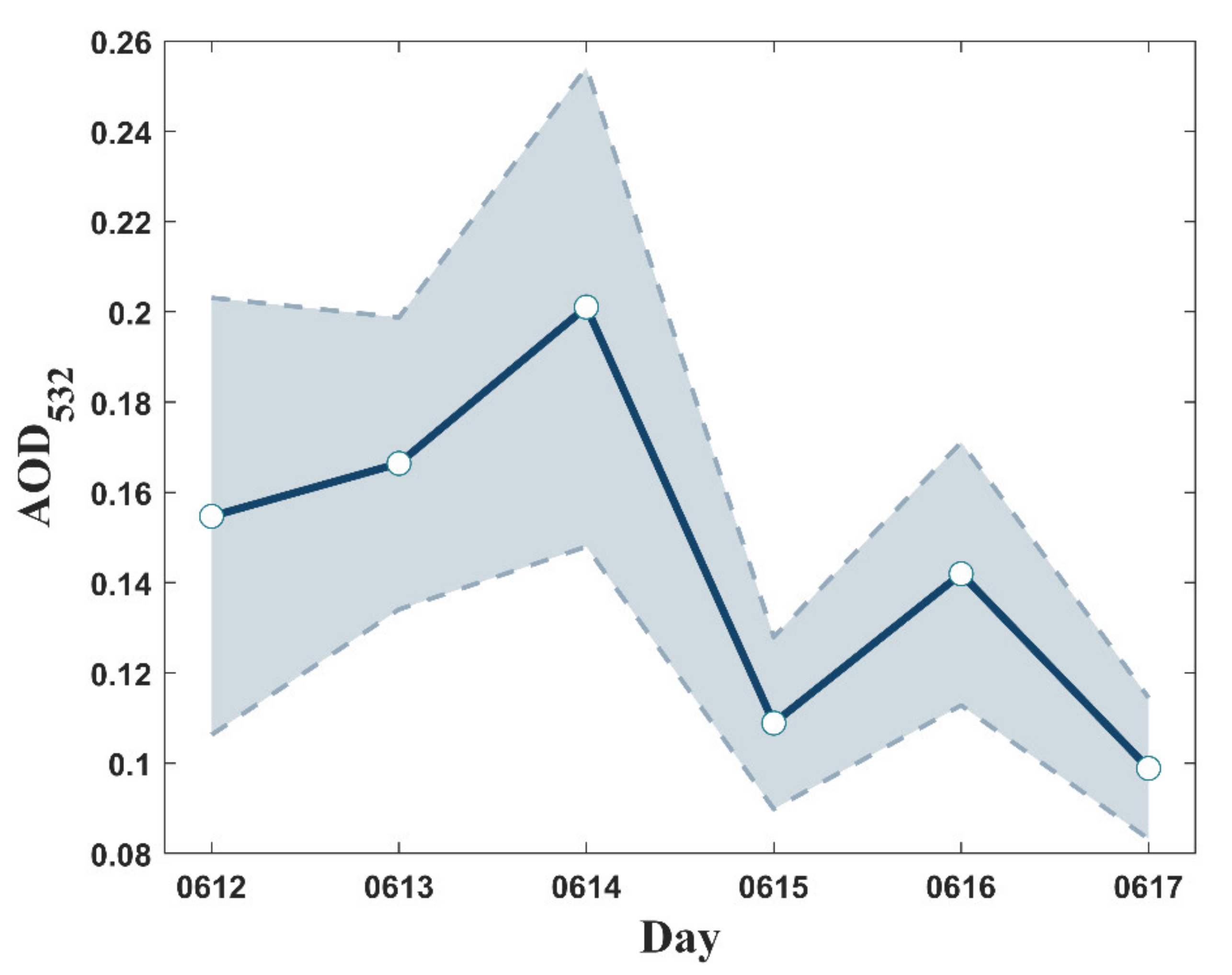
3.2.1. Daily Variations in AOD

In the course of this voyage, the scientific research ship experienced two passes of the frontal process in succession. The variation in AOD during this period is shown in Figure 5. With the southward movement of the front, the value of AOD increases from 12 to 14 June 2019 (BJT). When it comes to 14 June 2019, AOD increases gradually and eventually reaches the maximum of 0.25 at 17:00. Then, the mean value of AOD on 15 June 2019 drops to 0.11 at a sharp rate of 0.09 day⁻¹. Finally, AOD reaches a relative peak on 16 June 2019 before reverting to a low value again.

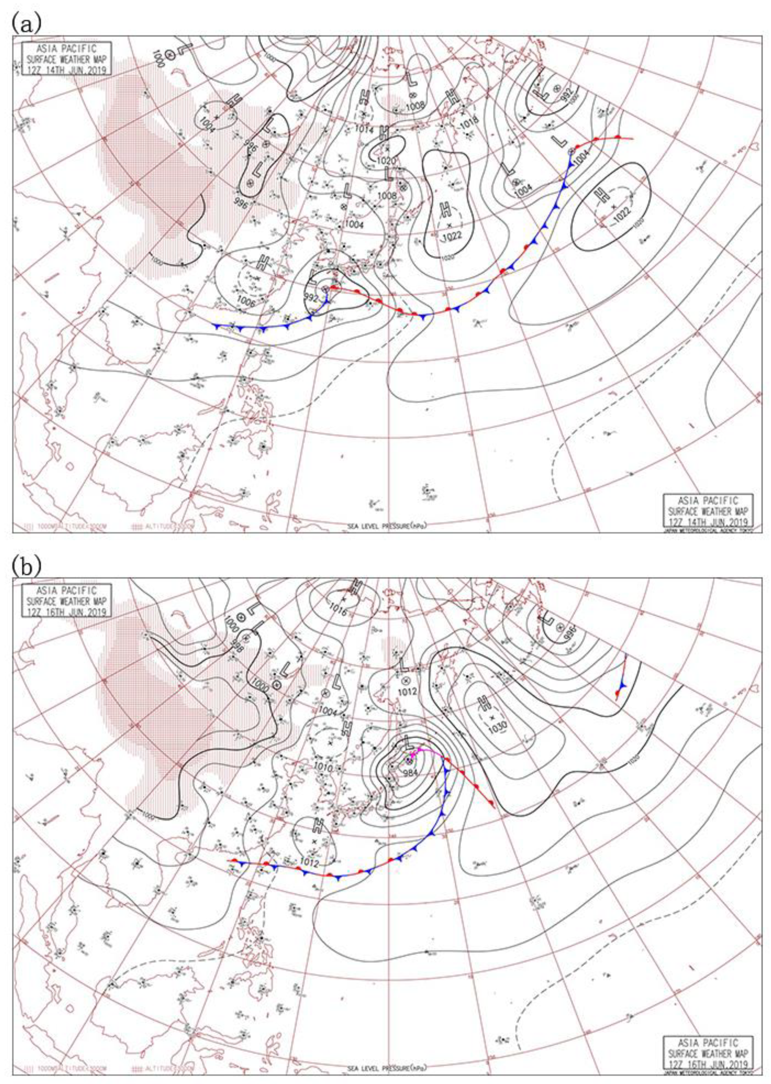
3.2.2. Synoptic Conditions and Their Influences

Like other meteorological quantities, AOD is highly sensitive to synoptic conditions. Figure 6 displays the surface synoptic patterns of frontal passages during the period. Before 20:00 13 June 2019, a quasi-stationary front is hovering over the Nan Ling Mountains of China. When it comes to 20:00, a center of low pressure appears along the coast of Fujian. At the same time, the quasi-stationary front turns into a cold front. As the low-pressure center moves eastward, the cold front continues to push southward and passes over the northern SCS at 08:00 14 June 2019. In addition, it arrives over the ship at about 18:00 14 June 2019, and the surface synoptic pattern at that time is depicted in Figure 6a. With the subtropical high moving southeast, the cold front on the sea converts back to a static front at about 08:00 15 June 2019 and then advances towards the Philippine Islands. However, this static front approaches in the opposite direction when the center of high pressure appears in the ocean. Finally, the research vessel Shen Kuo experiences a stationary front at about 17:00 16 June 2019, as indicated in Figure 6b.

Automatic weather stations, located on both sides of the ship, also captured these two processes. The variations in the measured meteorological elements are revealed in Figure 7. Before 14 June 2019, the wind speed rises promptly at an average rate of 1.64 m s⁻¹ day⁻¹. Temperature firstly increases and then decreases. In addition, a sudden drop in relative humidity and a sudden change in wind direction occur on 14 June 2019. These features are in conformity with the above surface weather map, indicating the passage of the cold front on 14 June 2019.

As demonstrated in Figure 7, the daily average wind speed of 14 June 2019 is the maximum. On this day, the number of hours with wind speed greater than 5 m s⁻¹ is up to 15, and the value at 07:00 even exceeds 10 m s⁻¹. The enhanced wind easily leads to the breaking of waves and the appearance of bubbles, due to the turbulent mixing of the ocean and atmosphere. After the bubble is broken and vaporized, these sea salt particles easily form aerosols. This contributes to the increment of sea salt aerosol concentration on the sea surface [60]. In addition, particle number densities with a radius greater than 0.50$\mathsf{\mu }\mathrm{m}$ on 14 June 2019 are much higher than those on other days (Figure 8). Furthermore, the relative contribution ratio of sea salt to the total AOD is also higher than other components on 14 June 2019, according to the dataset of MERRA-2. As a result, we deduce that these coarse particles, formed by the influence of enlarged wind, play a dominant role and then facilitate the rise of AOD [61]. This result is in line with the power-law relationship between wind speed and AOD found by Mulcahy et al. [62].

After the cold front passes through, the relative humidity drops to the minimum value of 78.68%, and the wind direction changes from southwest to northeast. It may transport some fine particles from nearby land. However, the low relative humidity would hinder the hygroscopic growth of aerosol particles. Integrated with the reduced wind speed, the value of AOD decreases. Later, with the influence of the quasi-stationary front, the rate of wind slightly augments, while relative humidity rapidly climbs to 84.66%. The high RH contributes to the heterogeneous aqueous reactions of NO₂ and hence enhances the level of nitrate particles in the atmosphere [63]. Furthermore, NH₄NO₃ in nitrate drives the increase in liquid water content and accelerates the hygroscopic growth [64]. Ultimately, the AOD value goes up. However, NH₄NO₃ is thermodynamically unstable. As the temperature rises from 16 to 17 June 2019, its stability is destroyed, and then the nitrate decreases, which is corroborated by the reduction in particle number densities in the accumulation mode. Additionally, the predominant southerly wind carries relatively clean ocean air mass. Under the joint influences of these two factors, AOD declines again.

3.2.3. The Thermal Structure

The concentration of particulate matter is closely related to the thermal structure, reflected by the temperature profile. As shown in Figure 9, there exists an inversion layer near the altitude of 650 m at 17:57 14 June 2019. After the passing of the cold front, the height of this inversion layer decreases, and then a shallow surface inversion layer appears at 00:01 15 June 2019. The downward trend of the inversion layer weakens the vertical diffusion ability of the atmosphere, boosting the enrichment of sea salt particles to a certain extent. This has been confirmed by the MERRA-2 dataset, in which the surface mass concentration of sea salt particles on 16 June 2019 is the maximum from 12 to 17 June 2019, with a value up to 1.78 × 10⁷ kg m⁻². As the altitude of the inversion layer rises on 15 June 2019, vertical diffusion conditions improve. However, this situation is changed on 16 June 2019. Compared with the elevation above 700 m at 23:56 on 15 June 2019, the inversion layer drops to around 300 m. This greatly encourages the aggregation of particles and then contributes to the amplification of AOD. With the quasi-stationary front passing through, the inversion layer disappears, and the value of AOD becomes lower.

As demonstrated in the cross sections of the extinction coefficient (Figure 10), the particle accumulation phenomenon caused by the inversion layer is very significant. Compared with 12 and 13 June 2019, the aerosol extinction coefficient has some disturbances in the upper layer on 14 June 2019, while the lower layer still maintains a high value. The high value mostly appears below 700 m, corresponding to the height of the inversion layer mentioned above at 17:57 14 June 2019. At the same time, the position of high values near the front transit (17:00 BJT) is lower and the value is higher than in the previous days, respectively. This high value is maintained for several hours, and the position continues to move downward, indicating that the vertical diffusion may be further reduced. Combined with the enrichment of sea salt particles, AOD increases on 14 June 2019. After the passage of the cloud front, the cross section of the extinction coefficient turns relatively cleaner. When it comes to 16 June 2019, there exists a brightness band in the stratification below 500 m at about 14:00 (BJT). The duration of this brightness band is longer and the thickness is larger than that on 15 June 2019. Therefore, the AOD value on that day is higher than that on the previous day. After the static front passes through, the brightness band of the bottom extinction coefficient dissipates and the AOD value decreases.

3.3. Temporal and Spatial Distribution of AOD

As an important parameter of atmospheric turbidity, the fluctuations of AOD reflect the variations in aerosol extinction ability to a certain extent. By studying the variation in AOD in weather processes or events, we can understand the main factors and specific physical and chemical mechanisms. At the same time, long-term research is also meaningful, because it can let us more accurately grasp the characteristics of the whole region and the implied law.

3.3.1. Validation of MERRA-2 and Measured Data

For many reasons, there are few conventional aerosol observations on the sea surface. It is impractical to study the long-term characteristics of aerosols over the ocean with a small amount of navigation data. Reanalysis products such as MERRA-2 datasets can make up for this gap. However, its artificial nature impacts the authenticity and effectiveness of its data, which still needs to be investigated. Therefore, validating the MERRA-2 reanalysis products with ground-based observations is quite crucial.

Figure 11 shows the comparison between the AOD products in the MERRA-2 reanalysis data and the AOD calculated by the observed extinction coefficient integration during the cruise. Both the daily average AOD of the reanalysis and the observation are applied for the validation. It is important to mention that almost all the points in the figure are scattered at the upper left of the 1:1 line, indicating that the AOD retrieved by MERRA-2 is greater than the corresponding observation. This overestimation has also been confirmed in previous studies [21,65]. The statistical evaluation of R = 0.44 also reveals that the performance of the MERRA-2 AOD product is mediocre. The divergence between MERRA-2 and ground observation may be caused by many factors [66]. It may be associated with the difference in sampling sensors fitted on the respective instruments [67], as well as measurement principles, such as the selection of satellite pixels and the method of reducing surface reflectance [68]. Nonetheless, previous studies [69,70,71] have shown that MERRA-2 can well characterize the AOD in the absence of other appropriate data. As a result, using MERRA-2 reanalysis data to study the spatiotemporal variations in AOD over the SCS is still practicable.

3.3.2. Spatial Variations in AOD

The spatial variations in AOD over the study region are collected by MERRA-2 atmospheric reanalysis data for the period from 2012 to 2021. The map of the annual average AOD is shown in Figure 12. Obviously, the AOD in this study area shows the characteristics of decreasing from northwest to southeast. The value varies from 0.02 to 0.56. Affected by the continental polluted air mass, the value of AOD in the offshore area is relatively high, especially in the Beibu Gulf area. The AOD declines noticeably as the offshore distance increases, eventually falling below 0.1 over the deep ocean.

Given the monsoon climate over the study region, it is of great value to clarify the spatial distributions in different seasons, as depicted in Figure 13. Here, four seasons are classified as followed: (1) spring (March, April and May); (2) summer (June, July and August); (3) autumn (September, October and November); (4) winter (December, January and February). Compared to other seasons, the AOD over the coastal area is exceedingly higher in spring, even exceeding 0.6 in some areas. It may be associated with the high intensity of biomass burning, such as forest fires or agricultural crop burning [72]. In contrast to spring, AOD in summer shows an obvious low value. Most AOD values in summer are below 0.25, mainly due to the southwest monsoon and the frequent rainfall settlement. The transport of pollutants from the continent to the ocean rises as the winter monsoon increases, resulting in an increase in AOD during the winter over the ocean.

3.3.3. Temporal Variations of AOD

The statistical results of the seasonal average AOD are shown in Figure 14a. The AOD in spring ranks the highest with a median of 0.26, followed by winter, autumn, and summer with their AOD of 0.24, 0.20, and 0.18, respectively. The characteristics of high AOD in spring and winter as well as low AOD in summer and autumn are intuitive, which is consistent with the seasonal variations observed by Wang et al. [73].

When it comes to the annual variations, the AOD is generally around 0.22. It is similar to the measured results over the Sanya Bay [73]. Among these years, the maximum value is −0.24 in 2016. Although the value fluctuates, the AOD over the study region decreases year by year, with a negative trend of −0.0027 year⁻¹. Additionally, the decline in AOD over eastern China is demonstrated by Proestakis E et al. [74], reflecting that the pollution is weakened. With the prevailing northward wind in the winter, the pollutants transported from eastern China to this region would become lesser and then easily contribute to the decrease in AOD. The results verify the effectiveness of China’s emission reduction policy.

3.3.4. Contribution of Components

To further understand the variations in AOD over the study region, it is critical to focus on the contributions of various aerosol compositions. In MERRA-2 aerosol products, five components are classified: sea salt, sulfate, black carbon, organic carbon, and dust, respectively. Here, black carbon and organic carbon are combined into one category of smoke. Annual and seasonal mean proportions of these components in AOD are illustrated in Figure 15. In terms of the annual contribution, sulfate and sea salt play a control role in AOD, with high ratios of 39.77% and 39.38%, respectively. Smoke accounts for 17.17%. The proportion of sand dust is the lowest, only 3.68%. The seasonal proportions of each component differ little from the annual average, except in spring. Compared with other seasons, the percentage of smoke in spring increased significantly, reaching 30.46%. The combined contributions of smoke and sulfate compositions bear responsibility for about 70% of the total AOD in spring. In addition, the ratio of dust AOD in spring reaches the maximum value, which is almost twice the annual average. It may be linked to the long-distance transport of dust aerosols from the Sahara and the deserts of northwest China [75]. The occurrence of these high proportions of components may be the reason for the high AOD in the spring mentioned above.

The fraction change in four components in the last ten years is exhibited in Figure 16. From 2012 to 2021, the mean contribution rate of smoke to AOD is maintained at around 0.17. The values of dust AOD range from 0.03 to 0.05 during the study period. Different from sulfate, smoke, and dust, the relative contribution of sea salt seems to increase year by year, but these four trends are not obvious. However, the contribution rates of sulfate and smoke show negative trends of −0.00077 year⁻¹ and −0.00043 year⁻¹, respectively, which indicates that the aerosol in the sea is reduced to a certain extent due to human activities. It should be noted that the component of nitrate is not involved in the MERRA-2 aerosol product. Tao et al. [76] discovered that turbulent mixing of residual aerosols, produced from low-level shallow stratocumulus clouds evaporating, contributes to the enhancement of nitrate mass concentrations. This suggests that MERRA-2 reanalysis still needs to be further improved.

4. Conclusions

In this study, the characteristics of aerosol particle size spectrum, extinction coefficient profile, and AOD over the SCS are investigated by the combined shipboard measurement from the South China Sea Monsoon Experiment and the reanalysis datasets from MERRA-2. The method of cloud recognition is applied to analyze the typical weather conditions during the cruise. In addition, mean, median, and standard deviation are used to describe the statistical characteristics of extinction coefficient, particle number concentration, and AOD. The major conclusions can be summarized as follows:

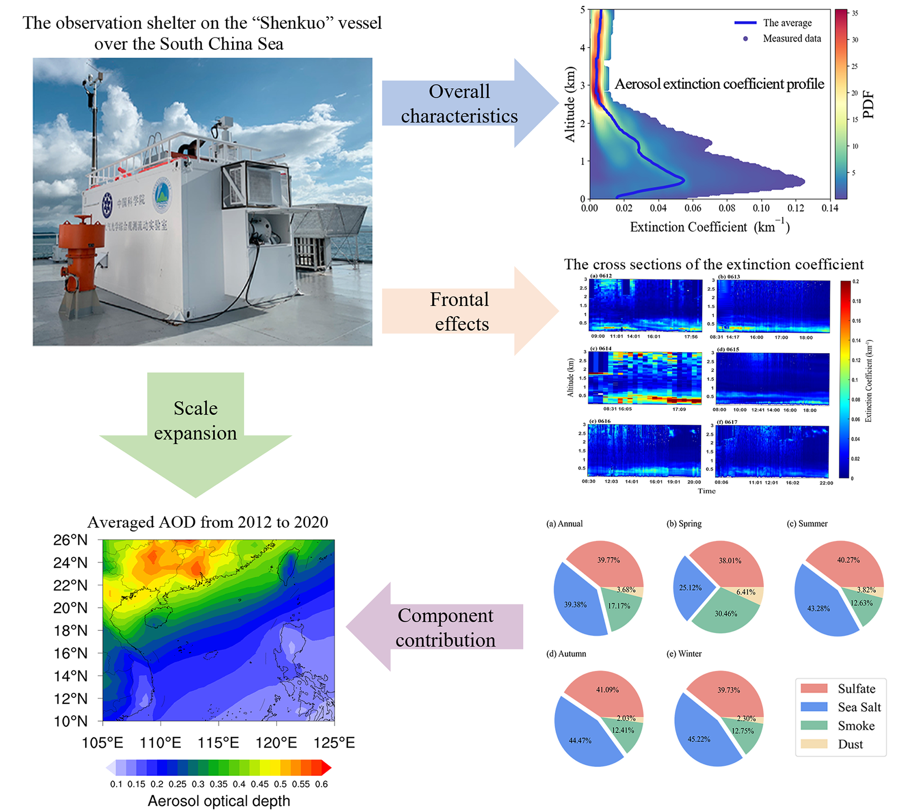
• For the weather conditions over the SCS, cloudless conditions rank first with a frequency of 47%. Single-layer cloud follows, and ice cloud with a high cloud base plays a leading role in this type. Therefore, the characteristics of aerosol extinction coefficients below 5 km are little disturbed by clouds, for the probability of clouds in this layer is low. Along with the uprising in altitude, the aerosol extinction coefficient increases rapidly and then falls after reaching the maximum value of 0.055 ${\mathrm{km}}^{-1}$ near 480 m. Furthermore, the value above 3 km attenuates below 0.02 ${\mathrm{km}}^{-1}$, indicating that aerosols in the atmosphere are mainly concentrated below 3 km.
• With the critical threshold being a radius of 0.50 $\mathsf{\mu }\mathrm{m}$, particles are composed of an accumulation mode as well as a coarse particle mode. The overall particle size spectrum conforms to the characteristics of the lognormal distribution. In addition, the two peaks of the volume spectrum are located at 0.10 and 1.00 $\mathsf{\mu }\mathrm{m}$, respectively.
• During the period of 12 to 17 June 2019, the scientific research ship experiences two weather processes: cold front and stationary front. These two frontal crossings result in the rise of AOD, due to which the former increases even more. Before the cold front passes, the enhanced wind easily leads to the breaking of waves on the sea surface and then facilitates the increment in sea salt aerosol concentration. These coarse particles dominate the total AOD. The reason for the increased AOD ahead of the quasi-stationary front is different from the cold front. Apart from the downward movement of temperature inversion, it may also be associated with the augmentation of nitrate concentration, due to low temperature as well as high relative humidity.
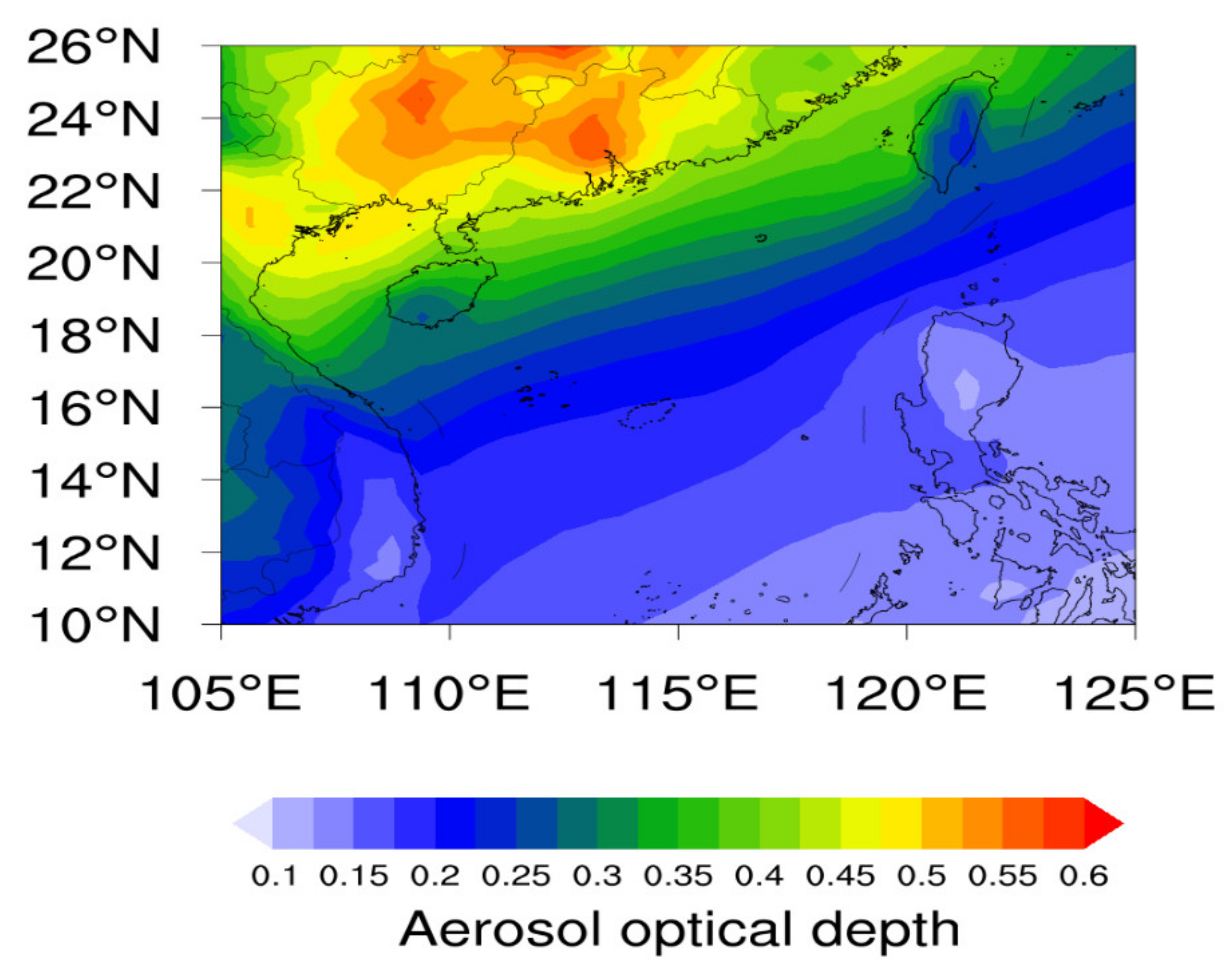
• For the region between 105°E–125°E and 10°N–26°N, the annual average AOD decreases from northwest to southeast. In addition, its obvious seasonality has been represented. AOD in spring ranks the highest with a median value of 0.26, followed by winter, autumn, and summer with 0.24, 0.20, and 0.18, respectively. The high AOD in spring may be closely related to the significant contributions of smoke and dust. Among four components, sulfate and sea salt play a leading role in AOD with average proportions of 39.77% and 39.38%, respectively. With the decline in sulfate and smoke, the total AOD in this region shows a significant negative trend of −0.0027 year⁻¹ from 2012 to 2021.

In general, marine aerosols in the SCS, dominated by fine particles such as sulfate, are greatly affected by coastal continents. However, the aerosol optical thickness has displayed an obvious decreasing trend in recent years, indicating that the concentration of marine aerosols has decreased. It should be noted that only three parameters, aerosol particle size distribution, aerosol extinction coefficient, and aerosol optical thickness, are involved in the discussion. To further understand the physical-optical properties of marine aerosols, more quantities, such as Angstrom exponent and refractive index, should be considered in the near future.

References

1. Arias, P.; Bellouin, N.; Coppola, E.; Jones, C.; Krinner, G.; Marotzke, J.; Naik, V.; Plattner, G.-K.; Rojas, M.; Sillmann, J.; et al. Climate Change 2021: The Physical Science Basis. Contribution of Working Group I to the Sixth Assessment Report of the Intergovernmental Panel on Climate Change; Technical Summary; Arias, P., Ed.; IPCC: Geneva, Switzerland, 2021. [Google Scholar]
2. Croft, B.; Martin, R.V.; Moore, R.H.; Ziemba, L.D.; Crosbie, E.C.; Liu, H.; Russell, L.M.; Saliba, G.; Wisthaler, A.; Müller, M.; et al. Factors controlling marine aerosol size distributions and their climate effects over the northwest Atlantic Ocean region. Atmos. Chem. Phys. 2021, 21, 1889–1916. [Google Scholar] [CrossRef]
3. Quinn, P.K.; Coffman, D.J.; Johnson, J.E.; Upchurch, L.; Bates, T.S. Small fraction of marine cloud condensation nuclei made up of sea spray aerosol. Nat. Geosci. 2017, 10, 674–679. [Google Scholar] [CrossRef]
4. Fossum, K.N.; Ovadnevaite, J.; Ceburnis, D.; Dall’Osto, M.; Marullo, S.; Bellacicco, M.; Simó, R.; Liu, D.; Flynn, M.; Zuend, A.; et al. Summertime Primary and Secondary Contributions to Southern Ocean Cloud Condensation Nuclei. Sci. Rep. 2018, 8, 13844. [Google Scholar] [CrossRef] [PubMed]
5. Luo, H.; Han, Y. Impacts of the Saharan air layer on the physical properties of the Atlantic tropical cyclone cloud systems: 2003–2019. Atmos. Chem. Phys. 2021, 21, 15171–15184. [Google Scholar] [CrossRef]
6. Liang, Z.; Ding, J.; Fei, J.; Cheng, X.; Huang, X. Direct/indirect effects of aerosols and their separate contributions to Typhoon Lupit (2009): Eyewall versus peripheral rainbands. Sci. China Earth Sci. 2021, 64, 2113–2128. [Google Scholar] [CrossRef]
7. Satheesh, S.; Moorthy, K.K. Radiative effects of natural aerosols: A review. Atmos. Environ. 2005, 39, 2089–2110. [Google Scholar] [CrossRef]
8. Bates, T.S.; Quinn, P.K.; Covert, D.S.; Coffman, D.J.; Johnson, J.E.; Wiedensohler, A. Aerosol physical properties and processes in the lower marine boundary layer: A comparison of shipboard sub-micron data from ACE-1 and ACE-2. Tellus B Chem. Phys. Meteorol. 2000, 52, 258–272. [Google Scholar] [CrossRef]
9. Raes, F.; Bates, T.; McGovern, F.; Van Liedekerke, M. The 2nd Aerosol Characterization Experiment (ACE-2): General overview and main results. Tellus B Chem. Phys. Meteorol. 2000, 52, 111–125. [Google Scholar] [CrossRef] [Green Version]
10. Smirnov, A.; Holben, B.N.; Slutsker, I.; Giles, D.M.; McClain, C.R.; Eck, T.F.; Sakerin, S.M.; Macke, A.; Croot, P.; Zibordi, G.; et al. Maritime Aerosol Network as a component of Aerosol Robotic Network. J. Geophys. Res. Earth Surf. 2009, 114, D06204. [Google Scholar] [CrossRef] [Green Version]
11. Chaubey, J.P.; Moorthy, K.K.; Babu, S.S.; Gogoi, M.M. Spatio-temporal variations in aerosol properties over the oceanic regions between coastal India and Antarctica. J. Atmos. Sol.-Terr. Phys. 2013, 104, 18–28. [Google Scholar] [CrossRef]
12. Liu, Y.; Yang, D.; Chen, W.; Zhang, H. Measurements of Asian dust optical properties over the Yellow Sea of China by shipboard and ground-based photometers, along with satellite remote sensing: A case study of the passage of a frontal system during April 2006. J. Geophys. Res. Earth Surf. 2010, 115, D00K04. [Google Scholar] [CrossRef] [Green Version]
13. Aswini, M.; Kumar, A.; Das, S.K. Quantification of long-range transported aeolian dust towards the Indian peninsular region using satellite and ground-based data—A case study during a dust storm over the Arabian Sea. Atmos. Res. 2020, 239, 104910. [Google Scholar] [CrossRef]
14. Ramana, M.V.; Devi, A. CCN concentrations and BC warming influenced by maritime ship emitted aerosol plumes over southern Bay of Bengal. Sci. Rep. 2016, 6, 30416. [Google Scholar] [CrossRef] [Green Version]
15. Breider, T.J.; Mickley, L.J.; Jacob, D.J.; Wang, Q.; Fisher, J.; Chang, R.; Alexander, B. Annual distributions and sources of Arctic aerosol components, aerosol optical depth, and aerosol absorption. J. Geophys. Res. Atmos. 2014, 119, 4107–4124. [Google Scholar] [CrossRef]
16. Aswini, A.; Hegde, P.; Aryasree, S.; Girach, I.A.; Nair, P.R. Continental outflow of anthropogenic aerosols over Arabian Sea and Indian Ocean during wintertime: ICARB-2018 campaign. Sci. Total Environ. 2019, 712, 135214. [Google Scholar] [CrossRef]
17. Ceamanos, X.; Six, B.; Riedi, J. Quasi-Global Maps of Daily Aerosol Optical Depth From a Ring of Five Geostationary Meteorological Satellites Using AERUS-GEO. J. Geophys. Res. Atmos. 2021, 126, e2021JD034906. [Google Scholar] [CrossRef]
18. Mallet, P.; Pujol, O.; Brioude, J.; Evan, S.; Jensen, A. Marine aerosol distribution and variability over the pristine Southern Indian Ocean. Atmos. Environ. 2018, 182, 17–30. [Google Scholar] [CrossRef]
19. Shi, C.; Hashimoto, M.; Nakajima, T. Remote sensing of aerosol properties from multi-wavelength and multi-pixel information over the ocean. Atmos. Chem. Phys. 2019, 19, 2461–2475. [Google Scholar] [CrossRef] [Green Version]
20. Sogacheva, L.; Popp, T.; Sayer, A.M.; Dubovik, O.; Garay, M.J.; Heckel, A.; Hsu, N.C.; Jethva, H.; Kahn, R.A.; Kolmonen, P.; et al. Merging regional and global aerosol optical depth records from major available satellite products. Atmos. Chem. Phys. 2020, 20, 2031–2056. [Google Scholar] [CrossRef] [Green Version]
21. Isaza, A.; Kay, M.; Evans, J.P.; Bremner, S.; Prasad, A. Validation of Australian atmospheric aerosols from reanalysis data and CMIP6 simulations. Atmos. Res. 2021, 264, 105856. [Google Scholar] [CrossRef]
22. Jin, S.; Ma, Y.; Zhang, M.; Gong, W.; Dubovik, O.; Liu, B.; Shi, Y.; Yang, C. Retrieval of 500 m Aerosol Optical Depths from MODIS Measurements over Urban Surfaces under Heavy Aerosol Loading Conditions in Winter. Remote Sens. 2019, 11, 2218. [Google Scholar] [CrossRef] [Green Version]
23. Huang, J.; Arnott, W.P.; Barnard, J.C.; Holmes, H.A. Theoretical Uncertainty Analysis of Satellite Retrieved Aerosol Optical Depth Associated with Surface Albedo and Aerosol Optical Properties. Remote Sens. 2021, 13, 344. [Google Scholar] [CrossRef]
24. Buchard, V.; Randles, C.A.; Da Silva, A.M.; Darmenov, A.; Colarco, P.R.; Govindaraju, R.; Ferrare, R.; Hair, J.; Beyersdorf, A.J.; Ziemba, L.D.; et al. The MERRA-2 Aerosol Reanalysis, 1980 Onward. Part II: Evaluation and Case Studies. J. Clim. 2017, 30, 6851–6872. [Google Scholar] [CrossRef]
25. Shao, S.; Qin, F.; Xu, M.; Liu, Q.; Han, Y.; Xu, Z. Temporal and spatial variation of refractive index structure coefficient over South China sea. Results Eng. 2020, 9, 100191. [Google Scholar] [CrossRef]
26. Smirnov, A.; Holben, B.N.; Kaufman, Y.J.; Dubovik, O.; Eck, T.F.; Slutsker, I.; Pietras, C.; Halthore, R.N. Optical Properties of Atmospheric Aerosol in Maritime Environments. J. Atmos. Sci. 2002, 59, 501–523. [Google Scholar] [CrossRef] [Green Version]
27. Zhang, C.; Xu, H.; Li, Z.; Xie, Y.; Li, D. Maritime Aerosol Optical and Microphysical Properties in the South China Sea Under Multi-source Influence. Sci. Rep. 2019, 9, 17796. [Google Scholar] [CrossRef]
28. Wang, S.-H.; Tsay, S.-C.; Lin, N.-H.; Chang, S.-C.; Li, C.; Welton, E.J.; Holben, B.N.; Hsu, N.C.; Lau, W.K.; Lolli, S.; et al. Origin, transport, and vertical distribution of atmospheric pollutants over the northern South China Sea during the 7-SEAS/Dongsha Experiment. Atmos. Environ. 2013, 78, 124–133. [Google Scholar] [CrossRef]
29. Geng, X.; Zhong, G.; Li, J.; Cheng, Z.; Mo, Y.; Mao, S.; Su, T.; Jiang, H.; Ni, K.; Zhang, G. Molecular marker study of aerosols in the northern South China Sea: Impact of atmospheric outflow from the Indo-China Peninsula and South China. Atmos. Environ. 2019, 206, 225–236. [Google Scholar] [CrossRef]
30. Xiao, H.-W.; Xiao, H.-Y.; Luo, L.; Shen, C.-Y.; Long, A.-M.; Chen, L.; Long, Z.-H.; Li, D.-N. Atmospheric aerosol compositions over the South China Sea: Temporal variability and source apportionment. Atmos. Chem. Phys. 2017, 17, 3199–3214. [Google Scholar] [CrossRef] [Green Version]
31. Tan, S.-C.; Shi, G.-Y.; Wang, H. Long-range transport of spring dust storms in Inner Mongolia and impact on the China seas. Atmos. Environ. 2012, 46, 299–308. [Google Scholar] [CrossRef]
32. Zhao, X.; Heidinger, A.K.; Walther, A. Climatology Analysis of Aerosol Effect on Marine Water Cloud from Long-Term Satellite Climate Data Records. Remote Sens. 2016, 8, 300. [Google Scholar] [CrossRef] [Green Version]
33. Sun, E.; Fu, C.; Yu, W.; Xie, Y.; Lu, Y.; Lu, C. Variation and Driving Factor of Aerosol Optical Depth over the South China Sea from 1980 to 2020. Atmosphere 2022, 13, 372. [Google Scholar] [CrossRef]
34. Randles, C.A.; Da Silva, A.M.; Buchard, V.; Colarco, P.R.; Darmenov, A.; Govindaraju, R.; Smirnov, A.; Holben, B.; Ferrare, R.; Hair, J.; et al. The MERRA-2 Aerosol Reanalysis, 1980 Onward. Part I: System Description and Data Assimilation Evaluation. J. Clim. 2017, 30, 6823–6850. [Google Scholar] [CrossRef]
35. Gelaro, R.; McCarty, W.; Suárez, M.J.; Todling, R.; Molod, A.; Takacs, L.; Randles, C.A.; Darmenov, A.; Bosilovich, M.G.; Reichle, R.; et al. The Modern-Era Retrospective Analysis for Research and Applications, Version 2 (MERRA-2). J. Clim. 2017, 30, 5419–5454. [Google Scholar] [CrossRef]
36. Feng, F.; Wang, K. Does the modern-era retrospective analysis for research and applications-2 aerosol reanalysis introduce an improvement in the simulation of surface solar radiation over China? Int. J. Climatol. 2019, 39, 1305–1318. [Google Scholar] [CrossRef]
37. Brooks, S.D.; Thornton, D.C. Marine Aerosols and Clouds. Annu. Rev. Mar. Sci. 2018, 10, 289–313. [Google Scholar] [CrossRef]
38. Kokhanovsky, A. Optical properties of terrestrial clouds. Earth-Sci. Rev. 2004, 64, 189–241. [Google Scholar] [CrossRef]
39. Zhang, J.; Li, Z.; Chen, H.; Yoo, H.; Cribb, M. Cloud vertical distribution from radiosonde, remote sensing, and model simulations. Clim. Dyn. 2014, 43, 1129–1140. [Google Scholar] [CrossRef]
40. Zhang, J.; Chen, H.; Li, Z.; Fan, X.; Peng, L.; Yu, Y.; Cribb, M. Analysis of cloud layer structure in Shouxian, China using RS92 radiosonde aided by 95 GHz cloud radar. J. Geophys. Res. Earth Surf. 2010, 115, 148–227. [Google Scholar] [CrossRef]
41. Fan, W.; Qin, K.; Xu, J.; Yuan, L.; Li, D.; Jin, Z.; Zhang, K. Aerosol vertical distribution and sources estimation at a site of the Yangtze River Delta region of China. Atmos. Res. 2018, 217, 128–136. [Google Scholar] [CrossRef] [Green Version]
42. Lewis, E.R.; Schwartz, S.E. Comment on “Size distribution of sea-salt emissions as a function of relative humidity”. Atmos. Environ. 2006, 40, 588–590. [Google Scholar] [CrossRef]
43. Zhang, K.M.; Knipping, E.M.; Wexler, A.S.; Bhave, P.V.; Tonnesen, G.S. Reply to comment on “Size distribution of sea-salt emissions as a function of relative humidity”. Atmos. Environ. 2006, 40, 591–592. [Google Scholar] [CrossRef]
44. Elterman, L. Relationships Between Vertical Attenuation and Surface Meteorological Range. Appl. Opt. 1970, 9, 1804–1810. [Google Scholar] [CrossRef]
45. Wang, Z.; Zhang, M.; Wang, L.; Feng, L.; Ma, Y.; Gong, W.; Qin, W. Long-term evolution of clear sky surface solar radiation and its driving factors over East Asia. Atmos. Environ. 2021, 262, 118661. [Google Scholar] [CrossRef]
46. Li, J.; Hu, Y.; Huang, J.; Stamnes, K.; Yi, Y. A new method for retrieval of the extinction coefficient of water clouds by using the tail of the CALIOP signal. Atmos. Chem. Phys. 2011, 11, 2903–2916. [Google Scholar] [CrossRef] [Green Version]
47. Kumar, N.M.; Venkatramanan, K. Lidar Observed Optical Properties of Tropical Cirrus Clouds Over Gadanki Region. Front. Earth Sci. 2020, 8, 140. [Google Scholar] [CrossRef]
48. Xia, X.; Che, H.; Zhu, J.; Cong, Z.; Deng, X.; Fan, X.; Fu, Y.; Goloub, P.; Jiang, H.; Liu, Q.; et al. Ground-based remote sensing of aerosol climatology in China: Aerosol optical properties, direct radiative effect and its parameterization. Atmos. Environ. 2015, 124, 243–251. [Google Scholar] [CrossRef]
49. Ramanathan, V.; Crutzen, P.J.; Lelieveld, J.; Mitra, A.P.; Althausen, D.; Anderson, L.M.; Andreae, M.; Cantrell, W.; Cass, G.R.; Chung, E.; et al. Indian Ocean Experiment: An integrated analysis of the climate forcing and effects of the great Indo-Asian haze. J. Geophys. Res. Earth Surf. 2001, 106, 28371–28398. [Google Scholar] [CrossRef]
50. Li, Y.; Wang, B.; Lee, S.-Y.; Zhang, Z.; Wang, Y.; Dong, W. Micro-Pulse Lidar Cruising Measurements in Northern South China Sea. Remote Sens. 2020, 12, 1695. [Google Scholar] [CrossRef]
51. Mascaut, F.; Pujol, O.; Verreyken, B.; Peroni, R.; Metzger, J.M.; Blarel, L.; Podvin, T.; Goloub, P.; Sellegri, K.; Thornberry, T.; et al. Aerosol characterization in an oceanic context around Reunion Island (AEROMARINE field campaign). Atmos. Environ. 2021, 268, 118770. [Google Scholar] [CrossRef]
52. Leeuw, G.D.; Andreas, E.L.; Anguelova, M.D.; Fairall, C.W.; Lewis, E.R.; O’Dowd, C.; Schulz, M.; Schwartz, S.E. Production flux of sea spray aerosol. Rev. Geophys. 2011, 49, RG2001. [Google Scholar] [CrossRef] [Green Version]
53. Lin, P.; Hu, M.; Wu, Z.; Niu, Y.; Zhu, T. Marine aerosol size distributions in the springtime over China adjacent seas. Atmos. Environ. 2007, 41, 6784–6796. [Google Scholar] [CrossRef]
54. Liang, B.; Cai, M.; Sun, Q.; Zhou, S.; Zhao, J. Source apportionment of marine atmospheric aerosols in northern South China Sea during summertime 2018. Environ. Pollut. 2021, 289, 117948. [Google Scholar] [CrossRef]
55. Painemal, D.; Chiu, J.-Y.C.; Minnis, P.; Yost, C.; Zhou, X.; Cadeddu, M.; Eloranta, E.; Lewis, E.R.; Ferrare, R.; Kollias, P. Aerosol and cloud microphysics covariability in the northeast Pacific boundary layer estimated with ship-based and satellite remote sensing observations. J. Geophys. Res. Atmos. 2017, 122, 2403–2418. [Google Scholar] [CrossRef]
56. Fitzgerald, J.W. Marine aerosols: A review. Atmos. Environ. Part A Gen. Top. 1991, 25, 533–545. [Google Scholar] [CrossRef]
57. Criscitiello, A.; Das, S.B.; Karnauskas, K.B.; Evans, M.; Frey, K.E.; Joughin, I.; Steig, E.J.; McConnell, J.R.; Medley, B. Tropical Pacific Influence on the Source and Transport of Marine Aerosols to West Antarctica. J. Clim. 2014, 27, 1343–1363. [Google Scholar] [CrossRef] [Green Version]
58. Hoppel, W.A.; Frick, G.M.; Fitzgerald, J.W.; Larson, R.E. Marine boundary layer measurements of new particle formation and the effects nonprecipitating clouds have on aerosol size distribution. J. Geophys. Res. Earth Surf. 1994, 99, 14443–14459. [Google Scholar] [CrossRef]
59. O’Dowd, C.D.; De Leeuw, G. Marine aerosol production: A review of the current knowledge. Philos. Trans. R. Soc. Lond. Ser. A Math. Phys. Eng. Sci. 2007, 365, 1753–1774. [Google Scholar] [CrossRef] [Green Version]
60. Lewis, E.R.; Schwartz, S.E. Measurements and Models of Quantities Required to Evaluate Sea Salt Aerosol Production Fluxes. In Sea Salt Aerosol Production: Mechanisms, Methods, Measurements and Models; Lewis, E.R., Schwartz, S.E., Eds.; American Geophysical Union: Washington, DC, USA, 2004; pp. 119–297. [Google Scholar] [CrossRef]
61. Kiliyanpilakkil, V.P.; Meskhidze, N. Deriving the effect of wind speed on clean marine aerosol optical properties using the A-Train satellites. Atmos. Chem. Phys. 2011, 11, 11401–11413. [Google Scholar] [CrossRef] [Green Version]
62. Mulcahy, J.P.; O’Dowd, C.D.; Jennings, S.G.; Ceburnis, D. Significant enhancement of aerosol optical depth in marine air under high wind conditions. Geophys. Res. Lett. 2008, 35, L16810. [Google Scholar] [CrossRef]
63. Trebs, I.; Meixner, F.X.; Slanina, J.; Otjes, R.; Jongejan, P.; Andreae, M.O. Real-time measurements of ammonia, acidic trace gases and water-soluble inorganic aerosol species at a rural site in the Amazon Basin. Atmos. Chem. Phys. 2004, 4, 967–987. [Google Scholar] [CrossRef] [Green Version]
64. Wu, X.; Li, M.; Chen, J.; Wang, H.; Xu, L.; Hong, Y.; Zhao, G.; Hu, B.; Zhang, Y.; Dan, Y.; et al. The characteristics of air pollution induced by the quasi-stationary front: Formation processes and influencing factors. Sci. Total Environ. 2019, 707, 136194. [Google Scholar] [CrossRef]
65. Mukkavilli, S.; Prasad, A.; Taylor, R.; Huang, J.; Mitchell, R.; Troccoli, A.; Kay, M. Assessment of atmospheric aerosols from two reanalysis products over Australia. Atmos. Res. 2018, 215, 149–164. [Google Scholar] [CrossRef] [Green Version]
66. Song, Z.; Fu, D.; Zhang, X.; Wu, Y.; Xia, X.; He, J.; Han, X.; Zhang, R.; Che, H. Diurnal and seasonal variability of PM2.5 and AOD in North China plain: Comparison of MERRA-2 products and ground measurements. Atmos. Environ. 2018, 191, 70–78. [Google Scholar] [CrossRef]
67. Sayer, A.M.; Hsu, N.C.; Lee, J.; Kim, W.V.; Dutcher, S.T. Validation, Stability, and Consistency of MODIS Collection 6.1 and VIIRS Version 1 Deep Blue Aerosol Data Over Land. J. Geophys. Res. Atmos. 2019, 124, 4658–4688. [Google Scholar] [CrossRef]
68. Aldabash, M.; Balcik, F.B.; Glantz, P. Validation of MODIS C6.1 and MERRA-2 AOD Using AERONET Observations: A Comparative Study over Turkey. Atmosphere 2020, 11, 905. [Google Scholar] [CrossRef]
69. Sun, E.; Che, H.; Xu, X.; Wang, Z.; Lu, C.; Gui, K.; Zhao, H.; Zheng, Y.; Wang, Y.; Wang, H.; et al. Variation in MERRA-2 aerosol optical depth over the Yangtze River Delta from 1980 to 2016. Arch. Meteorol. Geophys. Bioclimatol. Ser. B 2018, 136, 363–375. [Google Scholar] [CrossRef]
70. Khan, R.; Kumar, K.; Zhao, T.; Ullah, W.; de Leeuw, G. Interdecadal Changes in Aerosol Optical Depth over Pakistan Based on the MERRA-2 Reanalysis Data during 1980–2018. Remote Sens. 2021, 13, 822. [Google Scholar] [CrossRef]
71. Gueymard, C.A.; Yang, D. Worldwide validation of CAMS and MERRA-2 reanalysis aerosol optical depth products using 15 years of AERONET observations. Atmos. Environ. 2020, 225, 117216. [Google Scholar] [CrossRef]
72. Gautam, R.; Hsu, N.C.; Eck, T.F.; Holben, B.N.; Janjai, S.; Jantarach, T.; Tsay, S.-C.; Lau, W.K. Characterization of aerosols over the Indochina peninsula from satellite-surface observations during biomass burning pre-monsoon season. Atmos. Environ. 2012, 78, 51–59. [Google Scholar] [CrossRef]
73. Wang, Y.; Xin, J.; Li, Z.; Wang, S.; Wang, P.; Hao, W.M.; Nordgren, B.L.; Chen, H.; Wang, L.; Sun, Y. Seasonal variations in aerosol optical properties over China. J. Geophys. Res. Earth Surf. 2011, 116, D18209. [Google Scholar] [CrossRef]
74. Proestakis, E.; Amiridis, V.; Marinou, E.; Georgoulias, A.K.; Solomos, S.; Kazadzis, S.; Chimot, J.; Che, H.; Alexandri, G.; Binietoglou, I.; et al. Nine-year spatial and temporal evolution of desert dust aerosols over South and East Asia as revealed by CALIOP. Atmos. Chem. Phys. 2018, 18, 1337–1362. [Google Scholar] [CrossRef] [Green Version]
75. Wang, S.-H.; Tsay, S.-C.; Lin, N.-H.; Hsu, N.C.; Bell, S.; Li, C.; Ji, Q.; Jeong, M.-J.; Hansell, R.A.; Welton, E.J.; et al. First detailed observations of long-range transported dust over the northern South China Sea. Atmos. Environ. 2011, 45, 4804–4808. [Google Scholar] [CrossRef]
76. Tao, J.; Zhang, Z.; Tan, H.; Zhang, L.; Wu, Y.; Sun, J.; Che, H.; Cao, J.; Cheng, P.; Chen, L.; et al. Observational evidence of cloud processes contributing to daytime elevated nitrate in an urban atmosphere. Atmos. Environ. 2018, 186, 209–215. [Google Scholar] [CrossRef]
Figure 1. (a) the region of interest; (b) the cruise of Shen Kuo during June and July 2019; (c) the Shen Kuo research vessel; (d) the atmospheric optical comprehensive observation shelter on board.
Remotesensing 14 02453 g001
Figure 2. (a) Relative humidity profile at 00:04 28 June 2019 (BJT). The green line represents the original profile, while the blue line represents the revised profile. The red dotted line represents the height of 0 °C, and the brown line indicates the minimum humidity threshold. The purple areas represent the height at which the clouds appear; (b) the extinction coefficient profile at 00:02 28 June 2019 (BJT).
Remotesensing 14 02453 g002
Figure 3. Typical aerosol extinction coefficient profile in the period from 8 June to 2 July 2019. The blue solid line indicates the average aerosol extinction profile, while points on the graph denote the probability density of measured data.
Remotesensing 14 02453 g003
Figure 4. Particle size (a) number and (b) volume concentration distribution measured during the experiment from 8 June to 2 July 2019. Blue hollow dots represent the average number concentration at different radii. The pink area represents the standard deviation.
Remotesensing 14 02453 g004
Figure 5. Daily variations in AOD532 from 12 to 17 June 2019. Blue hollow dots represent the daily average AOD532, and the shadow represents the standard deviation.
Remotesensing 14 02453 g005
Figure 6. Surface weather maps at 20:00 BJT (UTC+8) on (a) 14th and (b) 16 June 2019. In these pictures, L represents the center of low pressure, while H represents high pressure. Blue lines with triangles refer to cold fronts, and the side of the triangle is in front of the front. In addition, the blue line on each side of the red-filled circle and the blue triangle represent the quasi-stationary front.
Remotesensing 14 02453 g006
Figure 7. Daily variations in meteorological elements during the period from 12 to 17 June 2019: (a) wind sped (m/s); (b) wind direction (°); (c) temperature (°C); (d) relative humidity (%). In addition, hollow dots represent the average values, while the shadows indicate the standard deviations.
Remotesensing 14 02453 g007
Figure 8. Daily particle size spectrum measured from 12 to 17 June 2019.
Remotesensing 14 02453 g008
Figure 9. Temperature profile measured at 5 times (BJT): 17:57 14 June 2019 (blue), 00:01 15 June 2019 (red), 23:56 15 June 2019 (yellow), 05:57 16 June 2019 (purple), 11:55 16 June 2019 (green). The dotted lines are the bottom heights of the inversion layer at the corresponding time.
Remotesensing 14 02453 g009
Figure 10. The cross sections of the extinction coefficient from 12 June to 17 June 2019.
Remotesensing 14 02453 g010
Figure 11. Scatter plot of MERRA-2 and the observations of AOD at 550 and 532 nm, respectively, during the voyage from 8 June to 2 July 2019. The purplish dotted line represents the 1:1 line. The red line represents the fitting curve. The correlations coefficient (R), the root mean square error (RMSE), and the mean absolute error (MAE) are indicated in the figure.
Remotesensing 14 02453 g011
Figure 12. The spatial distribution of the annual average AOD at 550 nm over the study region using the long-term MERRA-2 atmospheric products from 2012 to 2021.
Remotesensing 14 02453 g012
Figure 13. The spatial distributions of the seasonal average AOD at 550 nm over the study region using the long-term MERRA-2 atmospheric products from 2012 to 2021.
Remotesensing 14 02453 g013
Figure 14. (a) Box diagram of AOD at 550 nm in different seasons, in which the green triangles represent the average value. (b) Temporal variations in the annual mean AOD at 550 nm over the study region from 2012 to 2021. Note these data are from MERRA-2.
Remotesensing 14 02453 g014
Figure 15. Annual and seasonal mean proportions of AOD by four components: sulfate (red), sea salt (blue), smoke (green), and dust (orange). Note these data are from MERRA-2.
Remotesensing 14 02453 g015
Figure 16. Temporal variations in the annual mean proportion by four components: (a) sea salt; (b) sulfate; (c) smoke; (d) dust. The dotted lines represent the fittings of the trend.
Remotesensing 14 02453 g016