Article

Integrated Validation of Coarse Remotely Sensed Evapotranspiration Products over Heterogeneous Land Surfaces

1
State Key Laboratory of Earth Surface Processes and Resource Ecology, Faculty of Geographical Science, Beijing Normal University, Beijing 100875, China
2
Key Laboratory of Earth Surface Processes and Regional Response in the Yangtze-Huaihe River Basin, School of Geography and Tourism, Anhui Normal University, Wuhu 241000, China
3
Chongqing Survey Institute, Chongqing 400020, China
4
Hebei Technology Innovation Center for Remote Sensing Identification of Environmental Change, School of Geographic Sciences, Hebei Normal University, Shijiazhuang 050024, China
5
School of Resource and Environment, University of Electronic and Technology of China, Chengdu 611731, China
6
State Key Laboratory of Remote Sensing Science, Faculty of Geographical Science, Beijing Normal University, Beijing 100875, China
7
State Key Laboratory of Remote Sensing Science, Aerospace Information Research Institute, Chinese Academy of Sciences, Beijing 100101, China
*
Author to whom correspondence should be addressed.
These authors contributed equally to this work.
Remote Sens. 2022, 14(14), 3467; https://0-doi-org.brum.beds.ac.uk/10.3390/rs14143467
Submission received: 13 June 2022 / Revised: 11 July 2022 / Accepted: 15 July 2022 / Published: 19 July 2022
(This article belongs to the Special Issue Quantitative Remote Sensing Product and Validation Technology)

Abstract

:
Validation of remotely sensed evapotranspiration (RS_ET) products is important because their accuracy is critical for various scientific applications. In this study, an integrated validation framework was proposed for evaluating RS_ET products with coarse spatial resolution extending from homogenous to heterogeneous land surfaces. This framework was applied at the pixel and river basin scales, using direct and indirect validation methods with multisource validation datasets, which solved the spatial mismatch between ground measurements and remotely sensed products. The accuracy, rationality of spatiotemporal variations, and error sources of RS_ET products and uncertainties during the validation process were the focuses in the framework. The application of this framework is exemplified by validating five widely used RS_ET products (i.e., GLEAM, DTD, MOD16, ETMonitor, and GLASS) in the Heihe River Basin from 2012 to 2016. Combined with the results from direct (as the priority method) and indirect validation (as the auxiliary method), DTD showed the highest accuracy (1-MAPE) in the vegetation growing season (75%), followed by ETMonitor (71%), GLASS (68%), GLEAM (54%), and MOD16 (44%). Each product reasonably reflected the spatiotemporal variations in the validation dataset. ETMonitor exhibited the highest consistency with the ground truth ET at the basin scale (ETMap) (R = 0.69), followed by GLASS (0.65), DTD (0.63), MOD16 (0.62), and GLEAM (0.57). Error sources of these RS_ET products were mainly due to the limitations of the algorithms and the coarse spatial resolution of the input data, while the uncertainties in the validation process amounted to 15–28%. This work is proposed to effectively validate and improve the RS_ET products over heterogeneous land surfaces.

1. Introduction

Evapotranspiration (ET) is a keystone variable linking the water, energy, and carbon cycles [1]. Remotely sensed ET (RS_ET), which provides spatio-temporal continuous information over the land surface, can be beneficial to understand the water and energy budgets over different scales [2,3,4]. Recently, many RS_ET products have been released, such as the MODIS global ET (MOD16) [5], Global Land Evaporation Amsterdam Model (GLEAM) ET [6], Energy Balance ET (ET-EB) [7], Breathing Earth System Simulator (BESS) ET [8], Global LAnd Surface Satellite (GLASS) ET [9], Penman–Monteith–Leuning (PML_V2) [10], Operational Simplified Surface Energy Balance (SSEBop) [11], and ETMonitor [12] at the global scale, and the Satellite Application Facility on Land Surface Analysis (LSA-SAF) [13], Atmosphere Land Exchange Inverse (ALEXI) [14], Complementary-Relationship (CR-ET) [15], ETWatch [16], and Dual Temperature Difference (DTD) ET [17] at the regional or basin scale. However, there are significant differences between these coarse remotely sensed ET products from field to continent and global scales. The validation results indicated that the mean absolute percentage errors (MAPE) of RS_ET products can reach approximately 14–44, 9–35, and 5–21% at daily, monthly, and annual scales, respectively [2,3,11,18,19,20,21].
Currently, two types of validation approaches, direct and indirect validation, are widely used to assess the RS_ET products. The direct validation method can be conducted using the ground measurements from the eddy covariance (EC) system and scintillometer under homogeneous surfaces. The dearth of observations under heterogeneous surfaces makes it difficult to evaluate the accuracy of the coarse RS_ET without spatial mismatch. These complex surface conditions amplify the errors of the RS_ET products, validated by the fact that they have very inconsistent values [22,23]. However, the issues of the spatial mismatch between the satellite pixels and the measurement representation introduce unpredicted uncertainty into the evaluation report for the coarse RS_ET, especially under heterogeneous surfaces [24,25]. Therefore, it is essential to obtain the ground truth ET values by upscaling the in situ measurements to align with the spatial resolutions of the coarse satellite pixel [23,26,27,28,29].
The RS_ET products’ validation relies on comparison via a limited number of tower flux measurements under a homogenous surface. Although the values calculated from the water balance equation can assess this major element of the water cycle from river basin to global scale [25,30,31,32], the terrestrial ET calculated from the water balance equation provides only one value for a basin or hydrologic unit within a period, making it difficult to assess the rationality of the spatiotemporal distribution under various land cover types. The reliable spatial distribution of ET in a river basin could be estimated through upscaling the abundance of tower flux measurements from the major land cover types within it [33,34,35].
The indirect validation method includes the cross-validation of multiple ET products and evaluation of spatiotemporal consistency with ET-related variables. The cross-validation method can determine the differences and similarities in the magnitudes among ET products by inter-comparison with the ET from other RS_ET products, land surface models and reanalysis data [32,36,37,38]. Moreover, the rationality of spatiotemporal trends for RS_ET products can also be evaluated by characterizing the consistency with their influence factors, such as vegetation factors including the leaf area index (LAI) and normalized difference vegetation index (NDVI); meteorological factors including radiation, air temperature, humidity and wind speed; and land surface status including soil moisture.
Although many regional and global RS_ET products have been validated before release, the following are necessary for further improving their accuracy and helping users in better applying the RS_ET products: (1) extending the validation conducted from the homogenous to heterogeneous surface without the problem of spatial mismatch; (2) improving the RS_ET products’ assessment by integrating the approaches into a framework rather than being implemented individually; and (3) indicating the source of RS_ET errors is essential to the producer, and uncertainty of the validation results is necessary for users.
Under this context, this study proposes an integrated framework for coarse RS_ET products’ validation. The objectives are as follows: (1) to validate the RS_ET products under various heterogeneous land surfaces using the ground truth ET at the pixel and basin/regional scales; (2) to assess the RS_ET products using cross-validation and compare the trends with their influence factors; and (3) to demonstrate the accuracy of RS_ET products and their error sources, as well as the uncertainty of the validation process.

2. Study Area and Dataset

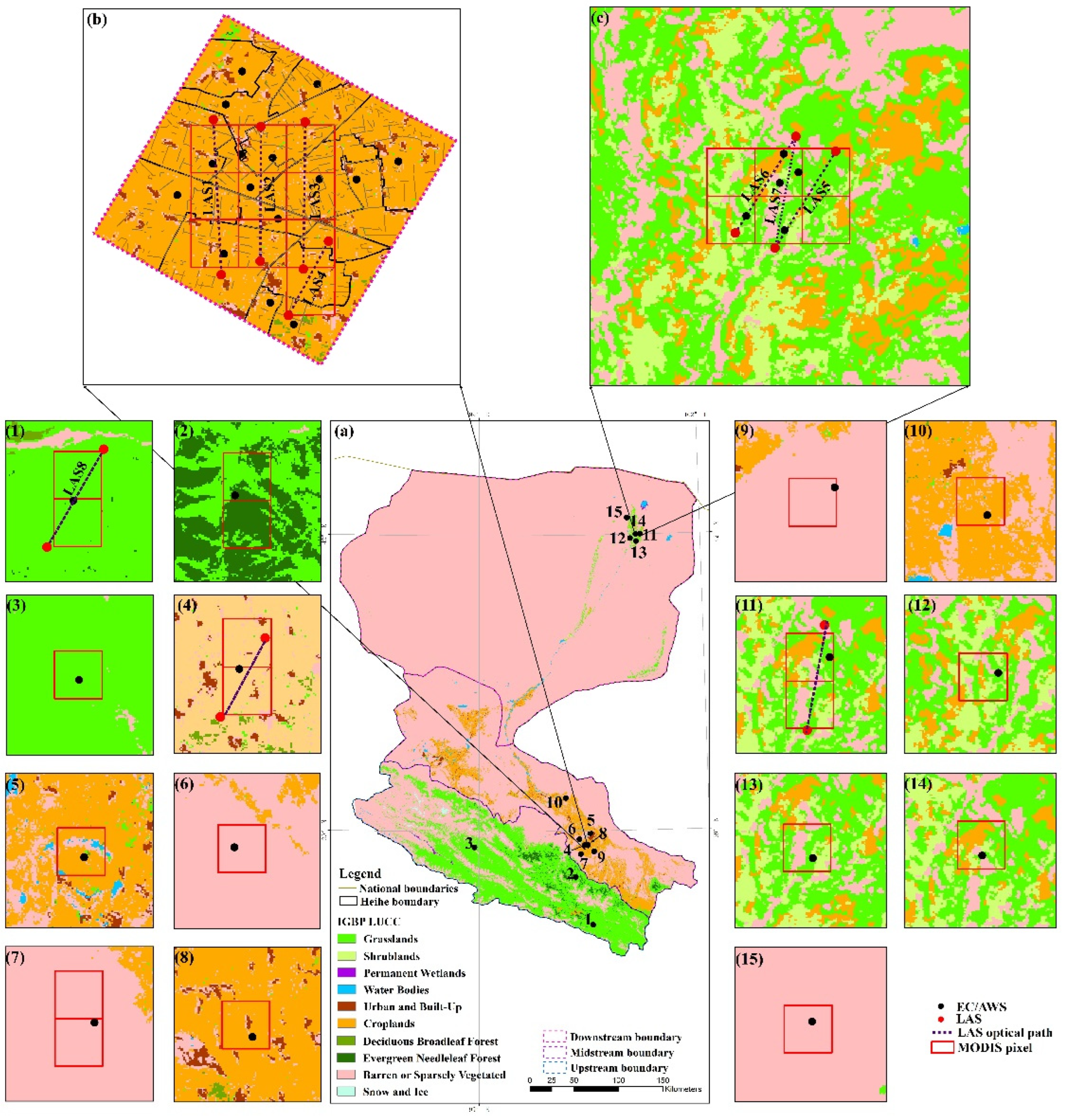
2.1. Study Area and Experiment

The Heihe River Basin (HRB), with an area of approximately 1.43 × 10⁵ km2 and located in the arid and semiarid regions of Northwest China, was selected as the study area. The HRB is a complicated watershed system with the coexistence of cold and arid regions and diverse landscapes [39] (shown in Figure 1). Over this basin, the mean annual air temperatures are 0.4, 7.3 and 8.2 °C, and annual precipitation is 322, 130 and 30 mm in the upstream, midstream and downstream regions, respectively [17]. In the upstream region, glaciers, permafrost, alpine meadows and forests are the dominant surface types. The midstream region is characterized by an artificial oasis (including farmland and shelter forests) and desert landscape. In the downstream region, the landscape is a natural oasis surrounding a large desert area, and riparian ecosystems are distributed along the river [40]. The HRB has diverse landscapes, which make it an ideal study area for the validation of RS_ET products from homogeneous to heterogeneous land surfaces.
The Heihe integrated observatory network was established in the HRB from 2007, during the WATER (Watershed Allied Telemetry Experimental Research) experiment (2007–2011 [41]), and was completed in 2013 during the HiWATER (Heihe Watershed Allied Telemetry Experimental Research) experiment (2012–2015 [39,42]). This network includes a maximum of 23 observation stations and it currently has 11 operating stations (three superstations and eight ordinary stations). Additionally, one other flux tower site (Linze site [43]) was used in the study. Figure 1a shows the flux tower site locations used in this study (site 1–15). From 3 May to 21 September 2012, the Multi-Scale Observation Experiment on Evapotranspiration over Heterogeneous Land Surfaces (MUSOEXE) was successfully conducted in the midstream of the HRB [23,44]. Two nested flux observation matrices were involved in HiWATER-MUSOEXE, including a large matrix (30 km × 30 km) and a kernel matrix (5.5 km × 5.5 km). The kernel matrix was initially divided into 17 sample plots (shown in Figure 1b) in the oasis. There was one EC system and one automatic weather station (AWS) in each plot to observe surface heat fluxes and meteorological elements [23]. There were four groups of large-aperture scintillometers (LAS) installed in the kernel matrix (the footprints of the LAS systems can cover three pairs of 3 × 1 MODIS pixels, named LAS1, LAS2 and LAS3 from west to east, respectively; one group covers one pair 2 × 1 MODIS pixels, named LAS4). Moreover, in the Ejina Oasis over the downstream region of the HRB, a flux observation matrix (3 km × 2 km) comprising five observation sites operated from 2013 to 2015. Two groups of LAS systems were installed in one pair of 2 × 2 MODIS pixels (LAS 5 and LAS6, shown in Figure 1c), which operated from 2013 to 2014, but the group of LAS located in one pair of 2 ×1 MODIS pixels (LAS7, shown in Figure 1c) left after 2015. In the upstream, there is one group of LAS and its footprint can cover one pair of 2 × 1 MODIS pixels (LAS 8, shown in Figure 1(a1)). Details of the observation instruments can be found in [23,39].

2.2. Remotely Sensed Evapotranspiration Products

In this study, five widely used coarse RS_ET products were evaluated according to the proposed ET validation framework. These ET products were grouped based on their intrinsic mechanisms: the first group included GLEAM [6] and DTD [17], which were derived from the surface energy balance; the second group included MOD16 [5] and ETMonitor [12], which were produced based on the eco-physiological processes of vegetation; the third group included GLASS [9], which was produced based on the integration of multiple algorithms. Details of the coarse RS_ET products are listed in Table 1. The DTD, ETMonitor and GLEAM ET products were aggregated to 8-day temporal resolution, while the GLEAM was resampled to 1-km spatial resolution.

2.3. Validation Dataset

2.3.1. Ground Truth ET

The ground truth ET at the satellite pixel scale will help to solve the spatial mismatch between ground measurements and RS_ET products. Depending on the heterogeneity of the land surface, the most appropriate methods were selected to acquire the ground truth ET at the satellite pixel scale using multiple flux tower measurements from June to September in the flux observation matrix of the midstream (LAS1-LAS4) during 2012 and the flux observation matrix of the downstream (LAS5-LAS7) during 2014–2015 in the HRB [26]. The dataset (daily, 1 km) can be downloaded from the National Tibetan Plateau Data Center (http://data.tpdc.ac.cn/ (accessed on 1 June 2018)).
Additionally, the satellite pixel-scale ground truth ET of the flux tower-located satellite pixels was also derived using the single flux tower measurements. The flux towers included three superstations (AR (Figure 1(a1)), DM (Figure 1(a4)) and SDQ (Figure 1(a11))) and twelve ordinary stations (GT (Figure 1(a2)), DSL (Figure 1(a3)), WD (Figure 1(a5)), BJT (Figure 1(a6)), HZZ (Figure 1(a7)), YK (Figure 1(a8)), SSW (Figure 1(a9)), LZ (Figure 1(a10)), PE (Figure 1(a12)), MF (Figure 1(a13)), BL (Figure 1(a14))) and DS (Figure 1(a15)) over typical underlying surfaces in the HRB [27]. The dataset (daily, 1 km) can be downloaded from the National Tibetan Plateau Data Center (http://data.tpdc.ac.cn/ (accessed on 10 December 2018)). The details of the ground truth ET at pixel scale are summarized in Table 2.
Regional ET at the watershed scale can be estimated by the water balance method, expressed as
E T = P R Δ S
where P is precipitation, R is runoff and ΔS is the change in terrestrial water storage. In this study, R was the difference in the water inflow and outflow, and ΔS was derived from the groundwater and reservoir storages. The water balance-based ET over the HRB during 2012–2016 was calculated according to these data with Equation (1) over the upstream, midstream and downstream, respectively. The results can be used as ground truth ET at the basin scale to validate RS_ET products. All the hydrologic data used in the water balance calculation were collected from the National Tibetan Plateau Data Center (http://data.tpdc.ac.cn/ (accessed on 10 December 2018)), which records data from hydrological observations over the HRB. Detailed information about the water balance calculation can be found in [45].
The ETMap was used as ground truth ET at the river basin scale to evaluate the RS_ET products under various land surfaces. The ETMap was obtained by applying the random forest method to train the daily ET and its explanatory variables over 36 flux tower sites (65 site years), and then we extended the results to the whole HRB. The variables related to ET, including leaf area index, solar radiation, precipitation, air temperature and relative humidity, were considered. The ETMap has spatial and temporal resolutions of 1 km and daily, respectively, from 2012 to 2016 [35], which can be downloaded from the National Tibetan Plateau Data Center (http://data.tpdc.ac.cn/ (accessed on 10 December 2018)).

2.3.2. ET Influence Factor Data and Auxiliary Dataset

The land cover map had a resolution of 30 m and high accuracy of over 90% [46]. Precipitation and air temperature datasets were used as influencing factors of ET to analyze the spatiotemporal trends of the RS_ET products. The 5 km/1 h atmospheric forcing dataset generated by Weather Research and Forecasting (WRF) [47] was used as the input of the hydrological-scale model in the HRB. The dataset of groundwater level was acquired by a downstream automatic water gauge in 2015. These datasets can be downloaded from the National Tibetan Plateau Data Center (http://data.tpdc.ac.cn/ (accessed on 10 December 2018)) [39].

3. Methodology

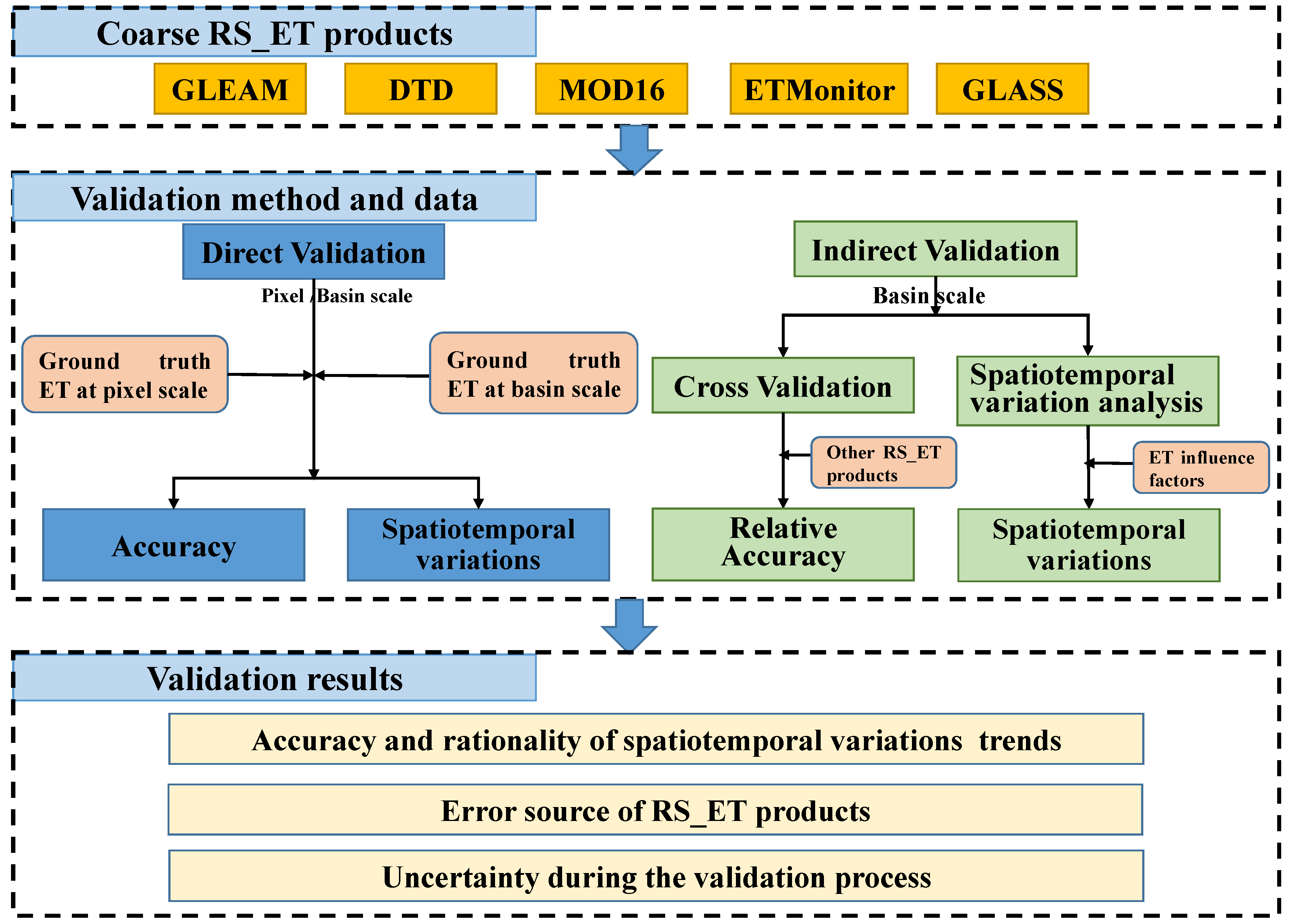
3.1. Validation Framework

The proposed validation framework has three progressive types of content, including the analysis of the accuracy and spatiotemporal variation trends of the RS_ET products, discussion of the error sources of the RS_ET products and assessment of the uncertainty in the validation process (Figure 2).
The first aspect of the framework is implemented to derive the accuracy of the RS_ET products using a direct validation method and indirect validation method. Specifically, in the direct validation method, the ground truth ET at the pixel and basin scales can be used to assess the accuracy and spatiotemporal trends of the RS_ET products. Meanwhile, in the indirect validation method, the three-cornered hat (TCH) approach is applied to obtain the relative accuracy among the RS_ET products at the basin scale, and the rationality of the spatiotemporal variations of the RS_ET products is explained by the ET impact factors. The second aspect involves tracking the error sources of the RS_ET products, which may be associated with the algorithms and the input datasets. Finally, the third aspect is to assess the uncertainty in the validation process using the generalized polynomial chaos (gPC) method [48].

3.2. Accuracy Evaluation Method

The Taylor diagram [49] was used to quantify the performance of the RS_ET products at the pixel scale. The Taylor diagram provides a suitable overview of the performance of different products in a single diagram by considering three statistics: the correlation coefficient (R), centered root mean square error (RMSE) and standard deviation (SD). Moreover, the mean absolute percentage error (MAPE) was utilized to quantify the accuracy of the RS_ET products. When validated by ETMap at the basin scale, the MAPE, BIAS and R were utilized to synthetically analyze the accuracy of the RS_ET products pixel by pixel in the HRB. The calculation methods for these evaluation indexes are listed in Appendix A.
For indirect validation, the TCH method was employed to evaluate the relative accuracy among these RS_ET products. This method is effective for characterizing the relative accuracy of more than three products. The TCH method relies on the removal of common signals from the RS_ET products and subsequently provides the relative errors [37,50]. The calculation result (variance) of TCH was squared and then divided by the average value of each product to obtain the relative error [27]. This is important to confirm the relative accuracy of the RS_ET products without ground truth ET. In this study, this method was employed to estimate the relative accuracy of five RS_ET products without any prior knowledge. The details of the TCH method are explained in Appendix C. Moreover, based on the ET impact factor data, such as the land cover type, air temperature and precipitation, the latitudinal profiles between RS_ET products and these factors were used to analyze the rationality of the spatiotemporal variation trend of the RS_ET products.

3.3. Uncertainty Evaluation Method

Quantitative evaluation of the uncertainty is an important part of the RS_ ET products’ validation. The EC measurements can represent the ground truth ET value at the pixel scale when the land surface is relatively homogeneous. Here, the uncertainty of ground truth ET is mainly determined by the ET observation error. In the method proposed by Beyrich [51], the maximum difference between LAS observations and EC observations, or the error of the EC measurements, is used to quantitatively evaluate the uncertainty of the ground truth ET at the pixel scale on a homogeneous underlying surface. When the land surface is moderately or highly heterogeneous, the uncertainty of the upscaled ground truth ET is mainly introduced from the errors of ET observation, auxiliary data and the upscaling method. In this study, the gPC method [48] was used to obtain the uncertainty introduced to the upscaled ground truth ET at the pixel scale [26,27]. The gPC method involves representing the inputs and outputs of a system under consideration through series approximations using standard random variables, thereby resulting in a computationally efficient means of uncertainty propagation through complex numerical models [52]. The gPC calculation result (variance) was squared and then was divided by the average value of ground truth ET at the pixel scale to obtain the uncertainty [27]. In this study, the input data, parameters and output data generated in the upscaling method are used to construct the polynomial chaos expansion model when calculating the uncertainty of the ground truth ET. The stochastic collocation method (SCM) is selected and treats the original model as a black box, and the coefficients of the polynomial chaos expansion terms are finally obtained by iteratively solving for selected collocation points in the input variables. Finally, the mean and variance output from the gPC method are used to calculate the uncertainty of the ground truth ET [27]. More details about the uncertainty quantification methods are given in Appendix D. For the ground truth ET at the basin scale (ETMap), the difference between ETMap values and LAS observations is calculated and then divided by the LAS observation [35], which can be used to determine the uncertainty of ground truth ET at the regional scale.

4. Validation Results of Coarse RS_ET Products

4.1. Direct Validation

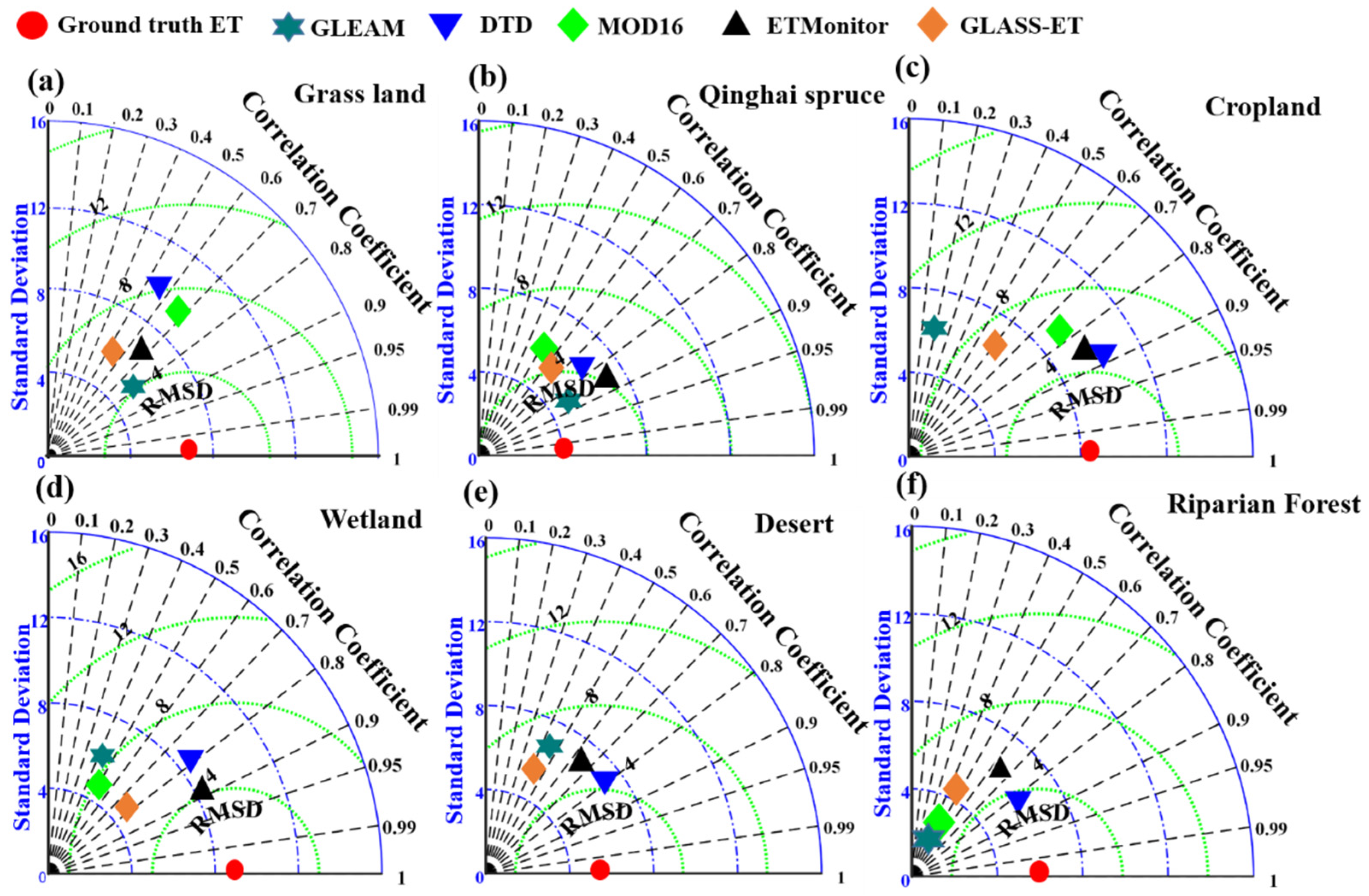
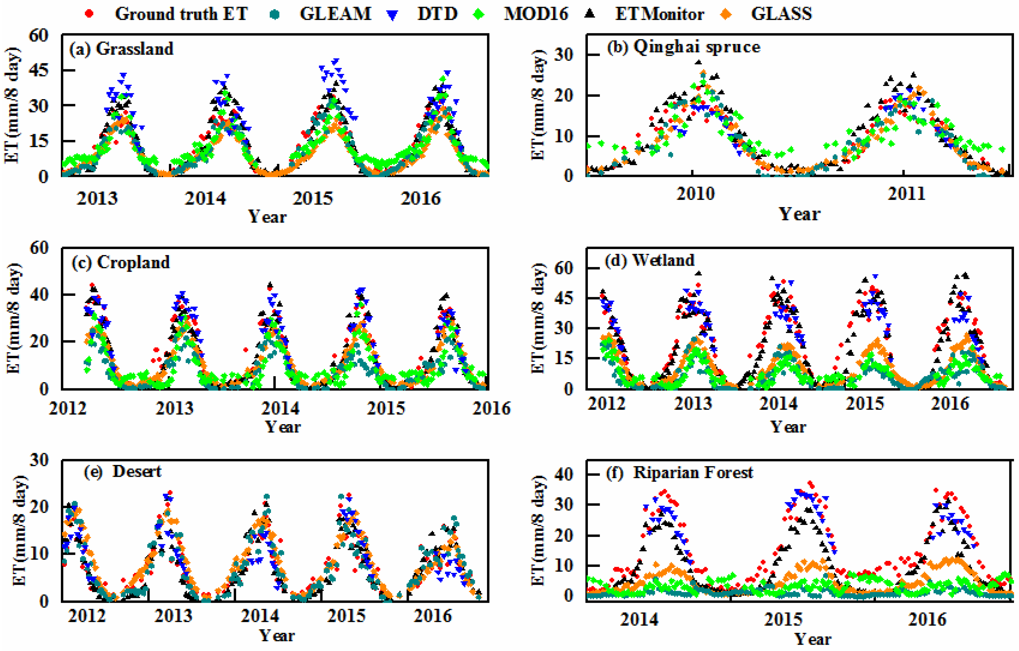
4.1.1. Validation at the Pixel Scale

The performance of the RS_ET products at the pixel scale was analyzed over six typical underlying land cover types, namely grassland, Qinghai spruce, cropland, wetland, riparian forest and desert, in the HRB. Grassland includes subalpine (represented by the AR site) and marsh alpine meadows (represented by the DSL site). Qinghai spruce (represented by the GT site) is an evergreen needle leaf forest and is the dominant land cover of forests in the HRB. The land cover of the cropland includes the DM and flux observation matrix in the midstream, YK and LZ sites. Wetland is represented by the WD site. In this study, barren land or sparsely vegetated areas belong to deserts (represented by the HZZ, BJT, SSW, DS and BL sites). Populus euphratica and Tamarix (belonging to deciduous broadleaf forest and shrub, respectively) in the downstream region are collectively called riparian forests (represented by the downstream flux observation matrix, SDQ, MF and PE sites). Figure 3 and Figure 4 show the Taylor diagrams and time series of the RS_ET products against the ground truth ET at the pixel scale, respectively. Table 3 presents the accuracy of the RS_ET products at the pixel scale, assessed by the MAPE during the vegetation growing season (from June to September) and the entire year.
At the pixel scale, the five RS_ET products exhibit differences in performance, especially during the growing season (Figure 3). The MAPE values of the whole year and the growing season were consistent (Table 3). Among these RS_ET products, ETMonitor and DTD performed better for most land cover types in the HRB, while GLEAM, MOD16 and GLASS performed well on Qinghai spruce, croplands or grasslands, respectively. According to the validation results, the MAPE value of the RS_ET products is relatively low on grassland, approximately ranging from 16.35 to 21.86% (in the growing season). In contrast, the RS_ET products had high MAPE values in the riparian forest, which ranged from 27.01 to 70.07% (in the growing season). The potential reason for this result might be that the grasslands are relatively uniform, while in the riparian forest, the land surface is more heterogeneous, and the RS_ET models would yield large errors.
Figure 4 shows the seasonal and inter-annual performance of the RS_ET products over typical land cover types. The five RS_ET products generally show similar seasonal and inter-annual variations and agree well with the ground truth ET, but the consistency is variable and associated with the land surface type. DTD and ETMonitor remained consistently better with ground truth ET in variation trends and magnitude over most land cover types. In general, the best agreement with ground truth ET at the pixel scale was found over the grassland, Qinghai spruce, and desert. Over the cropland, wetland, and riparian forest, their differences from the ground truth ET were obvious. Within a year, ET reaches its maximum value in July and August, and decreases to the minimum in winter. The variation trend of the DTD product has higher ET values in grasslands and it reached its peak in 2015 (50 mm/8 day), which was significantly higher than the ground truth ET. The MOD16 product overestimated the ET values in the non-growing season of 2010–2011 over Qinghai spruce, and the ET values in December and January were overestimated by approximately 8 mm/8 day. The seasonal variation amplitudes of GLEAM, MOD16, and GLASS over wetlands were significantly lower than the ground truth ET. For instance, in July and August, the values of these RS_ET products reached their peak of approximately 30 mm/8 day, while those of the ground truth ET reached 50 mm/mon. GLEAM and MOD16 showed significant underestimation; they are unable to accurately reflect the seasonal and inter-annual variation of ET over riparian forest. The value of GLEAM and MOD16 was approximately 10 mm/8 day during 2014–2016, while the ground truth ET could reach a peak value of 35 mm/8 day.

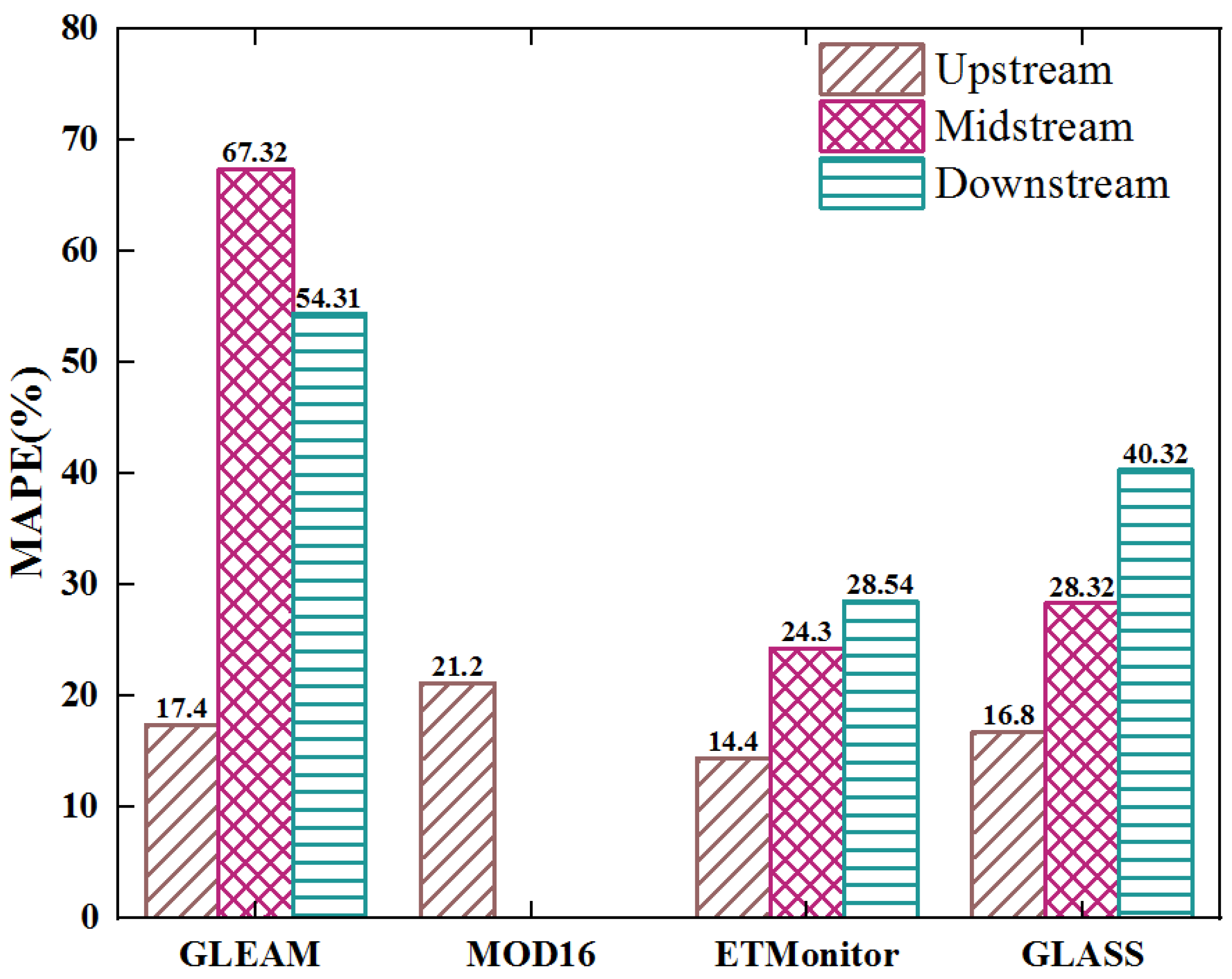
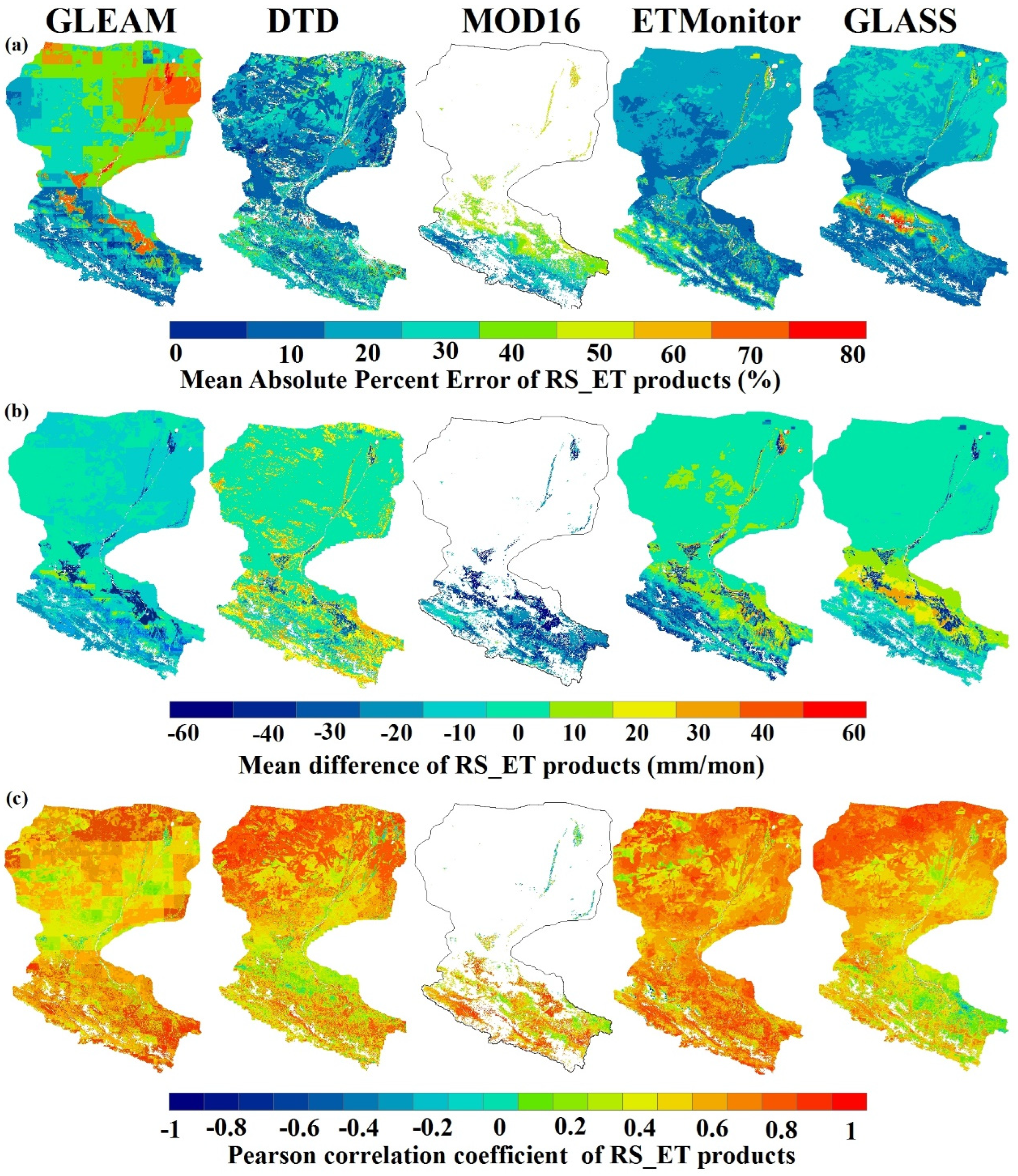
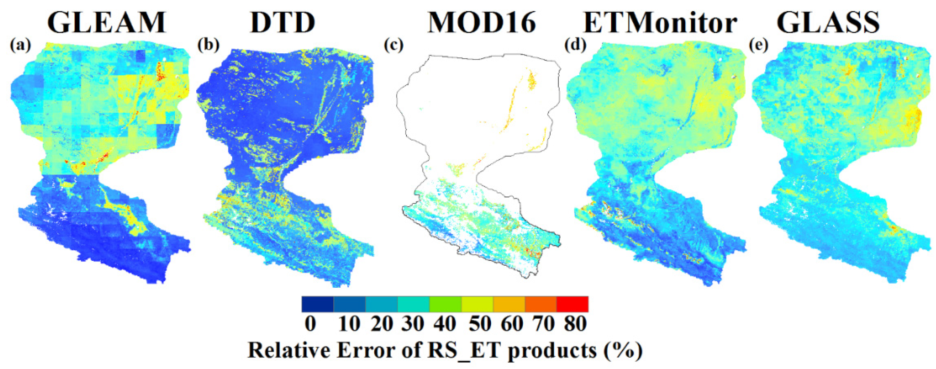
4.1.2. Validation at the Basin Scale

In the previous sections, differences in the magnitude of the RS_ET products at the pixel scale were observed. However, over heterogeneous surfaces, the pixel-scale validation results at limited sites may not represent the accuracy and spatiotemporal distribution pattern of the RS_ET products over the whole HRB. Therefore, it is necessary to conduct validation at the basin scale. The validation at the basin scale can be divided into two parts. First, the RS_ET products were validated using the watershed ET calculated by the water balance equation in the upstream, midstream, and downstream regions over the whole HRB, respectively. Second, the ground truth ET at the basin scale (ETMap) was used for the pixel-wise validation of the RS_ET products over the whole HRB.
Based on the ET calculated by the water balance equation in the upstream, midstream, and downstream regions, the validation results of GLEAM, GLASS, MOD16 (upstream), and ETMonitor are shown in Figure 5. All of the four RS_ET products performed best in the upstream region, with MAPE values less than 22%. In the midstream region, the MAPE values among these products are quite different, ranging from 24% for ETMonitor to 70% for GLEAM. In the downstream, the RS_ET products showed poor performance. ETMonitor, with a MAPE value of 28%, performed better than the other RS_ET products, and the MAPE values of GLASS and GLEAM were higher than 40%. Overall, ETMonitor exhibited better performance than other RS_ET products across the basin.
To analyze the pixel-wise product performance, further investigation was conducted by directly comparing each product with ETMap pixel by pixel over the whole basin. The spatial distributions of MAPE, BIAS (RS_ET—ETMap), and R of the RS_ET products are shown in Figure 6. We found that some conclusions were consistent with the above validation results. Over grassland areas, some pixels from DTD showed values of MAPE and BIAS higher than 30% and 20 mm/mon, respectively. DTD showed relatively low values of MAPE and BIAS in most cropland and riparian forest pixels. In contrast, the MAPE and BIAS of GLEAM showed relatively low values in most grassland and Qinghai spruce pixels, while these values increased over cropland and riparian forest. For MOD16, GLASS, and ETMonitor, values of MAPE and BIAS increased from upstream to downstream in most regions. Overall, each RS_ET product maintained good consistency with ETMap according to the high correlation coefficient values. The DTD had the lowest value of MAPE in the vegetation growing season (25%), followed by ETMonitor (29%), GLASS (32%), GLEAM (46%), and MOD16 (56%). ETMonintor tended to show certain underestimation (BIAS = −20 mm/mon), leading to a relatively high MAPE (MAPE > 30%) over the grassland. GLASS overestimated the ET in midstream desert regions (BIAS > 23 mm/mon). On the whole, DTD and ETMonitor exhibited better performance than other RS_ET products, with relatively low MAPE and BIAS values and high correlation coefficients in most pixels over the whole HRB.
The seasonal variation of ET values in typical land cover classes was compared between the RS_ET products and ETMap over the HRB, as shown in Figure 7. These comparisons show that all RS_ET products have captured the seasonal and inter-annual trends of ET relatively well against ETMap during most of the study period (2012–2016). DTD and ETMonitor have better consistency with ETMap in terms of magnitude and variation trend over most of the land cover types.
The largest inconsistencies were obtained over high-heterogeneity land surfaces such as riparian forest, especially for GLEAM, MOD16, and GLASS, and yielded negative bias. They produced peak ET values that were underestimated by nearly two times compared to the values of ETMap during the growing season. In 2012 and 2014, the peak value of DTD products was higher than that of ETMap over grassland, which was consistent with the results of the validation at the pixel scale. The ET values of GLASS had a certain overestimation in the desert during the non-growing season, while the GLEAM and MOD16 products underestimated the peak values over the cropland.

4.2. Indirect Validation

4.2.1. Cross-Validation

The cross-validation is implemented by using the TCH method to obtain the relative error among the five RS_ET products. The distribution of the relative error value for the RS_ET products is shown in Figure 8. The overall relative error variations can be generally listed as follows: grassland < Qinghai spruce < desert < cropland< wetland < riparian forest. The validation results of TCH were generally consistent with the results of the direct validation. Among the five RS_ET products, DTD exhibited better performance, achieving a low relative error value (lower than 22%) over the HRB, except for some grassland and Qinghai spruce pixels. Then, it was followed by ETMonitor (26%), which had relatively low relative error values in grasslands, Qinghai spruce, and croplands, but high relative error values in deserts and riparian forests. GLASS presented a moderate level of relative error in most pixels (approximately 30%) and had a high relative error in desert and riparian forests. GLEAM had a low relative error value in grassland and Qinghai spruce pixels (approximately 15%), while it had a high relative error value in cropland, desert regions, and riparian areas. MOD16 yielded a higher relative error in the HRB and it increased from upstream to downstream (greater than 35%).

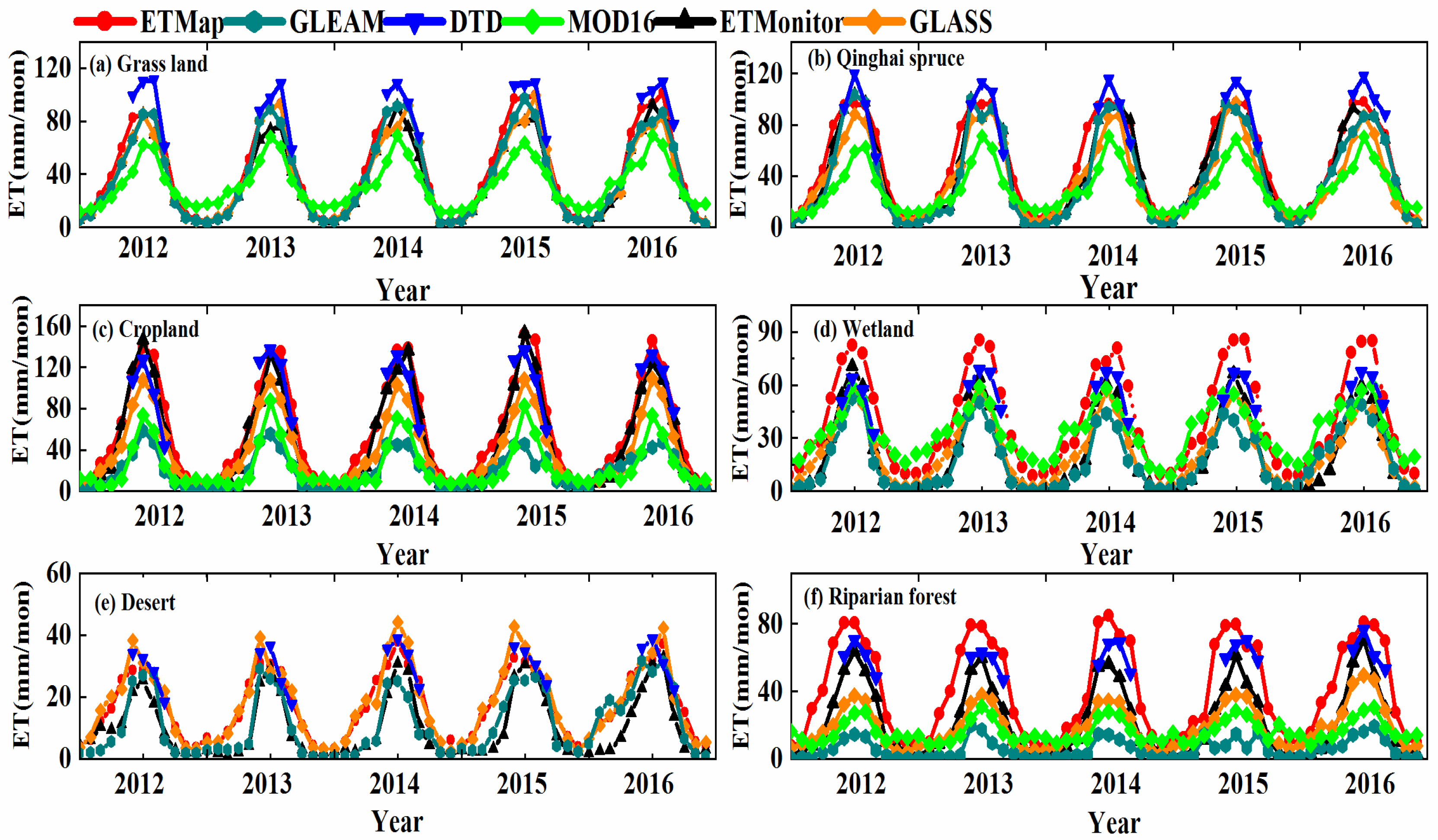
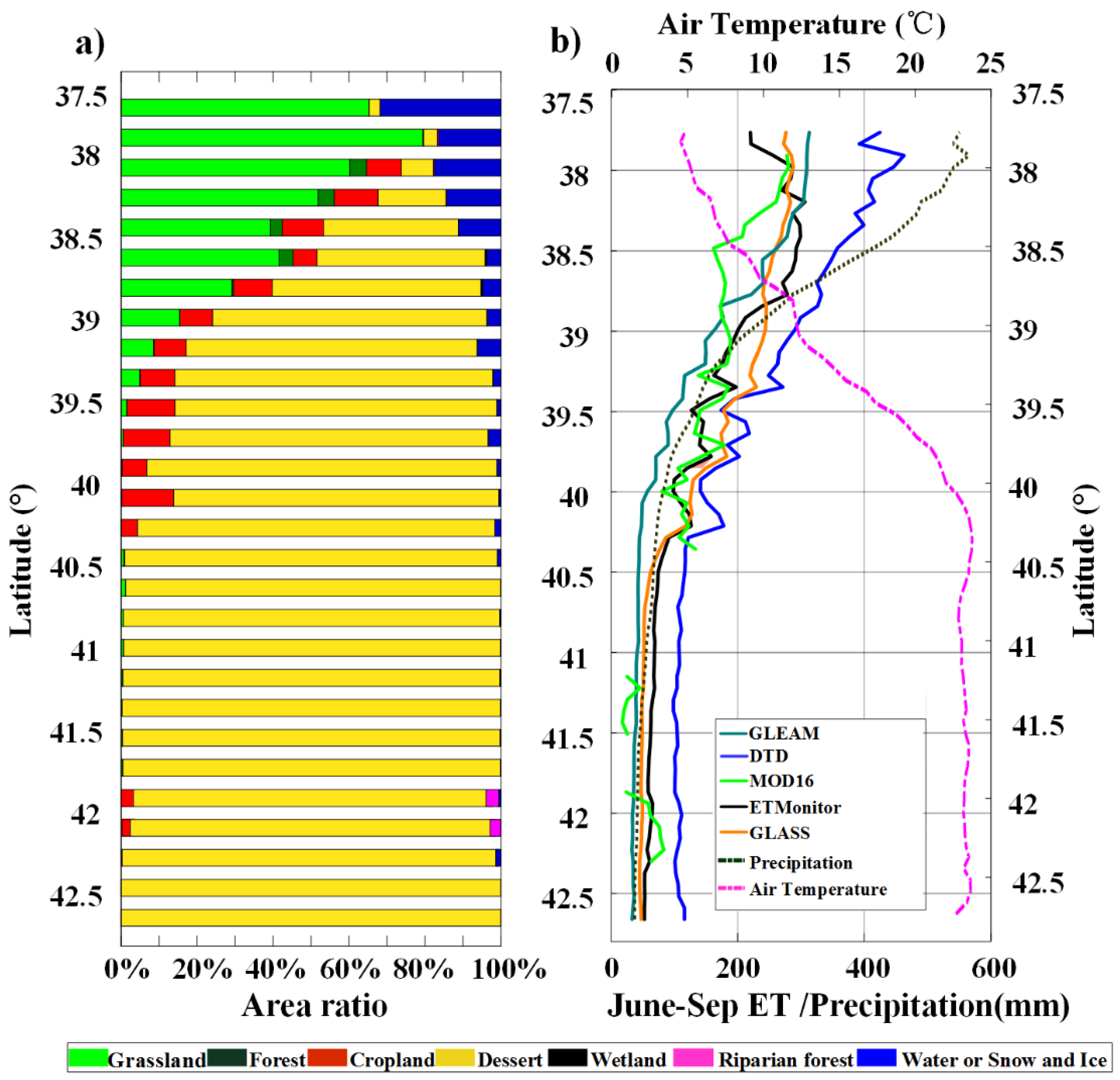
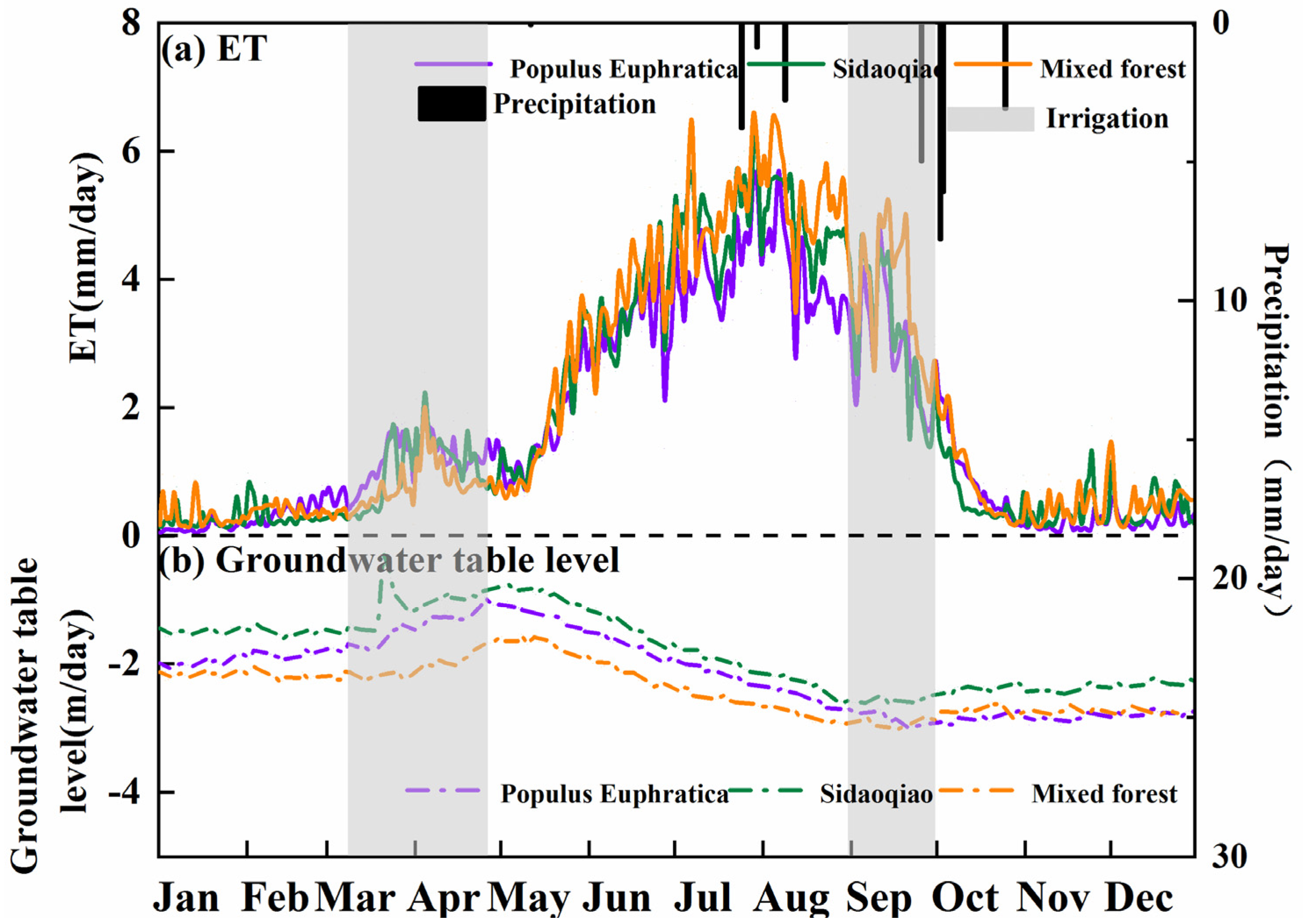
4.2.2. Spatiotemporal Variation Analysis

In this study, latitudinal profiles were adopted to analyze the rationality of the spatial–temporal changes among these products. The latitudinal profiles (Figure 9b) were drawn for the five RS_ET products along with the air temperature and precipitation. From upstream to downstream, with increasing latitude, the surface types changed from snow and ice, grassland/Qinghai spruce, cropland, and wetland/desert to riparian forest and cropland/desert. The air temperature values rose gradually and the precipitation and ET values decreased gradually, but high ET values were observed in the midstream and downstream oasis areas. The upstream region generates the runoff of the HRB; there is abundant precipitation over this area that results in greater precipitation than the ET. The midstream region consumed most of the water resources to irrigate the crops and yielded a higher ET than precipitation. There was rarely precipitation and low vegetation cover in the downstream region; thus, there were very low ET values over the broad desert but a slightly higher ET in the nature oases. All RS_ET products reasonably reflected the spatial changes in the ET values from upstream to downstream regions. The results also showed that MOD16 underestimated while DTD overestimated the ET values in the upstream region, respectively. GLEAM underestimated the ET in the downstream region, and it yielded an unreasonable result in which the rainfall was greater than the ET, even over the frequently irrigated agricultural areas.

5. Discussion

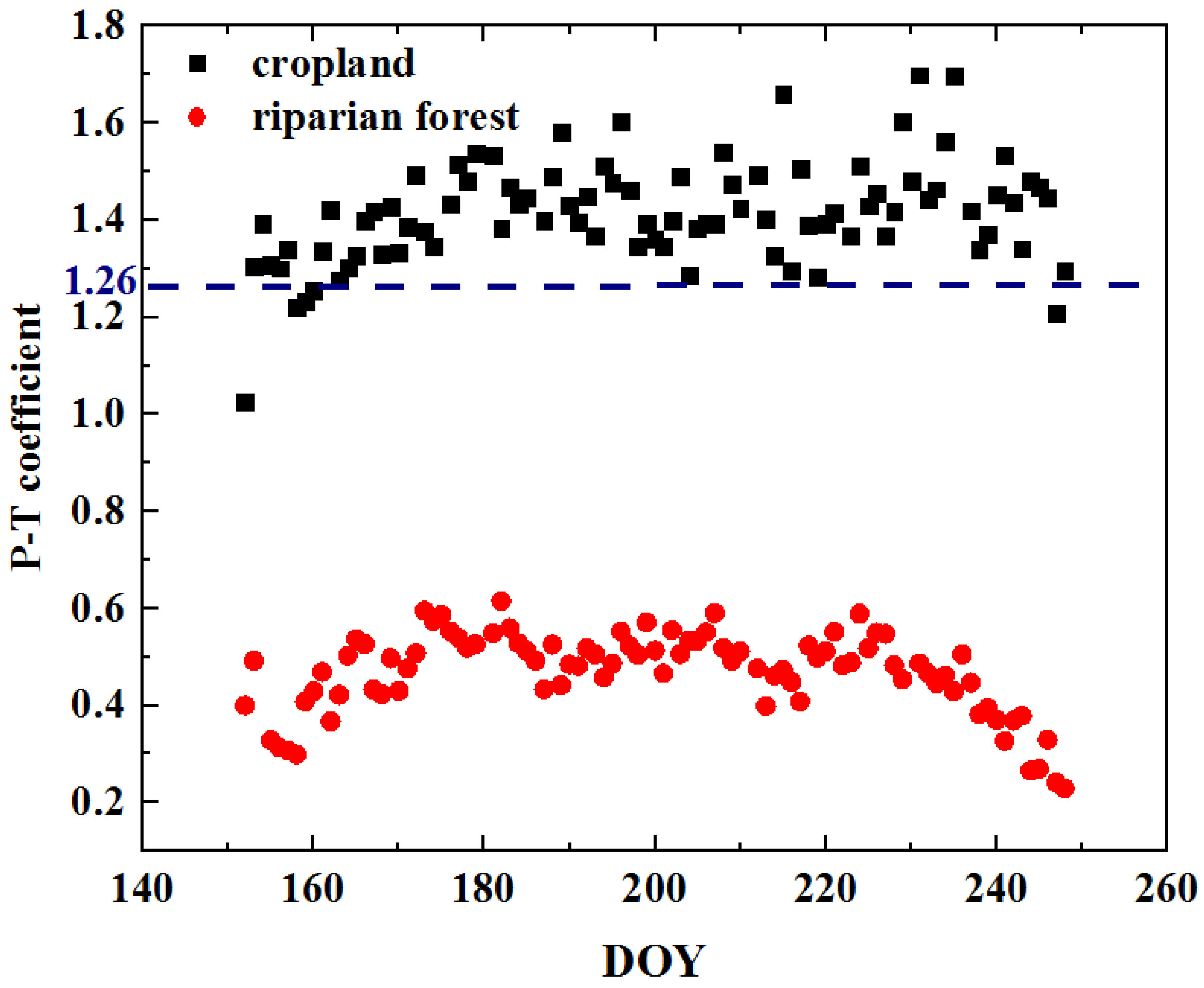
5.1. Error Sources of the RS_ET Products

The error sources of the RS_ET products are introduced in terms of two aspects: the limitations of the algorithm and errors of input data. For RS_ET products yielded based on the surface energy balance model, the largest limitation is the accuracy of the satellite-based land surface temperature (LST) data. Based on the validation results of DTD in the HRB, it exhibited obvious overestimation in the upstream region. A potential reason is that the suspected LST data were used in this model under cloudy and rainy weather conditions in the upstream region.
The validation of GLEAM showed an underestimation over the cropland and riparian forest (P. euphratica and Tamarix) in the downstream region, and it had a low correlation with ETMap over the cropland. In the GLEAM algorithm, a constant value of α = 0.8 was used to parameterize the tall canopy fraction, and a value of α = 1.26 was applied in both the short vegetation and bare soil fractions. However, previous studies have highlighted that α varies greatly over the growing season and with crop species, soil moisture availability, and climate conditions [53]. Here, we re-calculated the P-T coefficient values using the ground measurements at cropland (DM sites) and riparian forest (SDQ in the downstream) sites during the growing season (Figure 10). The results showed that the value of α varied with the land surface characteristics of different sites and was influenced by the seasonal variation. The value of α ranged from 1.2 to 1.8 at the DM site and from 0.2 to 0.6 at the SDQ site. The unreliable setting of the α value may potentially cause the discrepancy in GLEAM products over cropland and riparian forest pixels.
The eco-physiological process models often have difficulties in the parameterization of soil–plant–atmosphere interactions and other bio-physiological constraints [19]. MOD16 shows underestimation in most regions of the HRB. The parameterization of the MOD16 model is vital in controlling the ET; in particular, the surface resistance parameterization is essential to the model [4,54,55,56]. The application of VPD or relative humidity (RH) to represent the surface soil moisture status may be questionable. The VPD (or RH) is highly influenced by large-scale atmospheric conditions, while the soil moisture conditions over a large region are variable due to differences in precipitation, irrigation, underground water level, soil texture types, vegetation cover, and topography. Thus, the spatial variability of soil moisture can be stronger than that of VPD (or RH) [57].
ETMonitor is based on the physiological and ecological processes of vegetation, and it performed well over most land cover types in the HRB. However, it showed relatively low accuracy in the downstream region. This may due to the model having no corresponding mechanism to reflect the absorption of deep groundwater by vegetation, thus causing the underestimation of ETMonitor over riparian forests (such as P. euphratica and Tamarix). Figure 11 displays the groundwater table level and ET of the PE, SDQ, and MF sites in 2015. The groundwater level changes significantly within the range of 2–3 m and decreases immediately at the start of the growing season (June), due to the water consumed by the plants, along with increased ET values. This indicates that groundwater provides water for the ET over riparian forests (such as P. euphratica and Tamarix).
Relatively low accuracy was found in some desert and riparian forest pixels (P. euphratica and Tamarix) in the downstream. The ET accuracy of individual algorithms has a significant impact on the accuracy of the BMA method used in the production of GLASS. In the downstream region with sparse vegetation, each algorithm used in GLASS may not guarantee relatively high accuracy, thus affecting the overall integration accuracy. Moreover, using normal densities to calculate weights for the ET algorithms for different land cover types, without considering the weight differences for different growing seasons and climates, can also result in low accuracy [9].

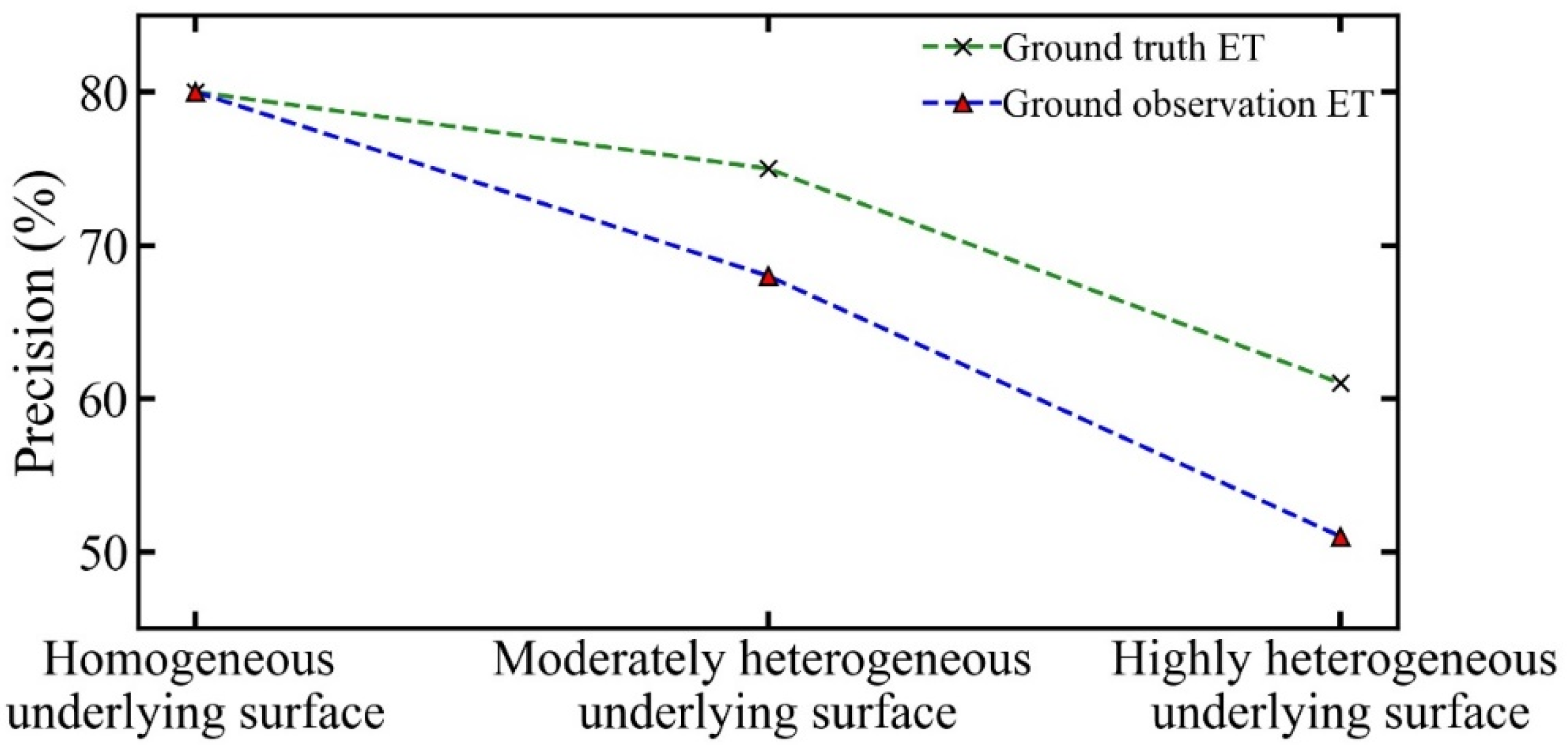
5.2. Uncertainties in the Validation Process

The RS_ET products have been validated using ground measurements, which are derived from the eddy covariance observations under a homogenous surface. However, this ignores the issue of spatial mismatch between the spatial representatives of the eddy covariance system and the image grid. Here, the ETmonitor with a spatial resolution of 1 km was assessed using the ground observation and ground truth ET, respectively, over a land surface ranging from homogenous to heterogeneous. This showed that they yielded very similar results under a homogenous surface, but their difference increased by as much as 10% when the land surface tended to be heterogeneous (Figure 12). This means that the ground truth ET urgently requires coarse RS_ET validation, especially for GLEAM. It has a spatial resolution of 0.25° but there are no ground measurements that possess a spatial representative to align with this coarse resolution. Hence, the GLEAM ET was resampled to 1 km and then validated using ground measurements and other RS_ET, which could have yielded unpredicted uncertainties during the validation.
Uncertainties associated with the validation process always exist but they have rarely been reported. The accuracy of the ground truth ET is primarily affected by the quantity, quality, and representativeness of the ET observation datasets [58]. EC measurements are important training data for ground truth ET [26,35]. It has been reported that the ET observation error from EC measurements ranges from 10 to 30 W/m2, and different EC data processing software show differences of 5 and 10% during flux data processing [59]. There are also errors yielded from ground observation-based ET upscaling, which is mainly related to the upscaling methods and their inputs. For example, in research by Li et al. [26] and Xu et al. [35], upscaling methods’ inputs, such as LST, LAI, and net radiation, were closely related to the accuracy of the upscaling results.
In this study, the method proposed by Beyrich et al. [51] was used to quantitatively evaluate the uncertainty of ground truth ET at the pixel scale under a homogeneous surface, while the gPC method was used for heterogeneous surfaces [26,27]. The uncertainty for ground truth ET at the pixel and regional scales is shown in Figure 13. We found that the uncertainty could be associated with the spatial heterogeneity of the land surface, which is consistent with recent studies [23,27]. EC measurements and ground observation-based ET upscaling methods tend to have relatively high accuracy in relatively homogeneous land cover types, such as grasslands and deserts, which had lower uncertainties in our study (15–18%). Over heterogeneous land cover types, such as wetlands and riparian forests, the error of EC measurements and upscaling methods tends to increase, reaching values as high as 22% to 28%. Moreover, the uncertainty (MAPE) of ETMap throughout the basin is approximately 20.69% when compared with LAS observations, which can represent the ground truth ET at satellite pixels [35].

6. Conclusions

In this study, a validation framework was established to evaluate RS_ET products extending over homogenous to heterogeneous land surfaces. The validation framework was applied to assess the GLEAM, DTD, MOD16, ETMonitor, and GLASS products from 2012 to 2016 in the HRB. The main conclusions are summarized as follows.
First, a validation framework was proposed for evaluating coarse RS_ET products over heterogeneous land surfaces with multisource validation datasets (ground truth ET at the pixel and basin scales, other RS_ET products, and ET impact factors), multiple validation methods (direct and indirect validation methods), and multiple scales (pixel and basin scales). In this validation framework, we report the accuracy and the rationality of the spatiotemporal variations of the RS_ET products, the error sources of the products, and the uncertainty of the validation process.
Second, the validation results were consistent among the direct and indirect methods at different scales. The DTD had the highest accuracy (1-MAPE) in the vegetation growing season (75%), followed by ETMonitor (71%), GLASS (68%), GLEAM (54%), and MOD16 (43.59%). All RS_ET products had the capability to maintain the consistency of the spatiotemporal trends of ET and its impact factors. ETMonitor and DTD performed relatively well (with R values higher than 0.66), followed by MOD16 (0.62) and GLASS (0.65), and, finally, GLEAM (0.57). These validation results could also be affected by the accuracy of the ground truth ET dataset. The results showed that the uncertainty of the ground truth ET at the pixel scale was approximately 15% over relatively homogeneous land surfaces, while it can be up to 28% over highly heterogeneous land surfaces.
Validating coarse RS_ET products over heterogeneous surfaces is still a critical research issue. The validation framework proposed in this study could contribute to understanding the accuracy and rationality of spatiotemporal variations in the RS_ET products over heterogeneous surfaces, promoting their application. In the future, we could apply this validation framework and ground truth ET acquisition method at the pixel/basin scale over more climates, surface types, and regions.

Author Contributions

Conceptualization, S.L.; methodology, Y.Z. and L.S.; software, Y.Z.; validation, Y.Z., L.S. and S.L.; formal analysis, Y.Z., L.S. and S.L.; investigation, Y.Z., L.S. and S.L.; resources, Y.Z., L.S. and S.L.; data curation, Y.Z., S.L. and G.H.; writing—original draft preparation, Y.Z and L.S.; writing—review and editing, X.L., Z.J., T.X., Z.X., Y.M., J.Z., X.Y., X.H. and Y.Y.; visualization, Y.Z.; supervision, S.L.; project administration, S.L.; funding acquisition, S.L. All authors have read and agreed to the published version of the manuscript.

Funding

This research was funded by the Strategic Priority Research Program of the Chinese Academy of Sciences, grant number XDA20100101, and the National Natural Science Foundation of China, grant number 41531174.

Data Availability Statement

All datasets in the Heihe River Basin were obtained from the National Tibetan Plateau Data Center (http://data.tpdc.ac.cn (accessed on 10 December 2018)).

Acknowledgments

The authors would like to thank all the scientists, engineers, and students whoparticipated in WATER and HiWATER field campaigns. We appreciate all reviewers and editors for their comments on this paper.

Conflicts of Interest

The authors declare no conflict of interest.

Appendix A

The mean absolute percent error (MAPE), root mean square error (RMSE), bias, and correlation coefficient (R) were used to show the accuracy and the rationality of the spatiotemporal trends of the RS_ET products. They are expressed as follows:
M A P E = 100 n i = 1 n | P i O i | O ¯
R M S E = i = 1 n ( P i O i ) 2 / n  
B I A S = i = 1 n ( P i O i ) / n
R = i = 1 n ( P i P ¯ ) ( O i O ¯ ) / [ i = 1 n ( P i P ¯ ) 2 i = 1 n ( O i O ¯ ) 2 ] 1 / 2
where P i represents the RS_ET product, O i is the ground truth ET at the pixel or regional scale, P ¯ is the mean RS_ET value,   O ¯ is the mean ground truth ET, and n is the number of samples.

Appendix B

The input data of the coarse RS_ET products used in this study are presented in Table A1.
Table A1. Summary of the coarse RS_ET product inputs.
RS_ET ProductTypeVariableDatasetSpatial
Resolution
Temporal
Resolution
GLEAMAtmospheric forcing dataPrecipitationTMPA 3B42v70.25°1 day
TaAIRS L3RetStdv6.03 h
Remote sensing dataRadiationCERES L3SYN1DEG1 day
Snow–water equivalentGLOBSNOW L3av2+ NSIDC V0.10.25°1 day
VODSMOS-LPRM25 km1 day
Soil moistureSMOS L325 km1 day
Cover fractionsMOD44B250 m1 year
Soil propertiesIGBP-DIS0.25°1 year
Lightning frequencyLIS/OTD5 km1 month
DTDAtmospheric forcing dataTa/Ws/q/RadiationThe atmospheric forcing data in the Heihe River Basin5 km1 h
Remote sensing dataLSTMODIS1 km1 day
AlbedoMODIS1 km1 day
LAIMODIS/GLASS1 km8 days
MOD16Atmospheric forcing dataTa/Tmin/
FPAR/q
GMAO/MERRA GMAO0.5° × 0.6°/
1.00° × 1.25°
1 day
Remote sensing dataFPAR/LAIMODIS500 m8 days
Albedo500 m8 days
Land cover500 m1 year
ETMonitorAtmospheric forcing dataTa/q/Ws/RadiationThe atmospheric forcing data in the Heihe River Basin5 km1 h
Remote sensing dataLAI/NDVIMODIS1 km16 days
Albedo1 km8 days
LST1 km1 day
Land coverMICLCover1 km1 year
PrecipitationTRMM0.25°1 day
Soil propertiesChina dataset of soil hydraulic parameters1 km
Soil moistureCCI25 km1 day
GLASSAtmospheric forcing dataTa/Tmin/
Tmax/q/WS/Radiation
GMAO-MERRA0.5° × 0.667°1 day
Remote sensing dataLAI/FPARMODIS/
AVHRR
1 km8 days
NDVI/EVI0.05°16 days
Albedo500 m1 day
Land coverUMD Land Cover Classification1 km1 year
Note: Ta refers to the air temperature, Tmax refers to the maximum temperature, Tmin refers to the minimum temperature, q refers to the atmosphere-specific humidity, WS refers to the wind speed, LST refers to the land surface temperature, LAI refers to the leaf area index, NDVI refers to the normalized vegetation index, FPAR refers to the fraction of absorbed photosynthetically active radiation, and VOD refers to the vegetation optical depth.

Appendix C

In the three-cornered hat (TCH) method, five RS_ET products were stored in the array { X i } i = 1 , 2 , , N , where N (N = 5) is the number of RS_ET products, and 𝑖 is the ith RS_ET products. Any RS_ET product can be expressed as
X i = X t + ε i ,       i = 1 , 2 , , N
where X t is the true value and ε i is the error of the ith time series. The symbol ∀ is called the universal quantifier. As no true estimate of X t is available, any single time series is arbitrarily chosen as the reference. The series of differences matrix can be obtained by calculating the difference between each time series and the reference. The corresponding covariance matrix S of the series of difference matrices is thus obtained. Notably, the valuation of uncertainties is not related to the selection of the reference series.
The unknown N × N covariance matrix of the individual noise R is introduced, and R is related to S as follows:
S = J · R · J T
where J is described as follows:
J N 1 , N = [ 1 0 0 1 0 1 0 1 0 0 0 1 ]
Equation (A6) cannot be solved as the number of equations is less than the number of unknowns (when N is greater than 3). Therefore, the remaining free parameters require a reasonable method to obtain a unique solution. Galindo and Palacio (1999) [60] proposed a constraint function to meet | R | > 0 as follows:
  H ( r 1 N , ,   r N N ) = | R | | S | · K < 0
where r 1 N , ,   r N N are the elements of the corresponding R and K = | S | N 1 is introduced to better obtain a numerical solution.
This constraint function constrains the free parameters within the solution domain but is insufficient to determine a unique solution for the free parameters. The following objective function is also used to provide the optimal selected criterion to obtain the unique parameter solution as follows:
F ( r 1 N , , r N N ) = 1 K 2 · i < j N r i j 2
R is calculated using the objective function under the constraint condition by combining it with Equation (A6). The uncertainty of the time series { X i } i = 1 , 2 , , N , denoted { σ i } i = 1 , 2 , , N , can be obtained by calculating the square root of the diagonal values in R (i.e., { r i i } i = 1 , 2 , , N ). The relative uncertainty is the ratio of σ i to the mean X i .

Appendix D

According to the method of Beyrich et al. [23], the uncertainty of the ground truth ET over a homogeneous underlying surface is calculated via
Δ ET = max ( σ r ,   abs ( ET _ EC ET LAS ) )
where ∆ET represents the uncertainty of the ground truth ET, ET_EC represents the ET observed by EC, ETLAS represents the LAS observed value, and σr represents the error of the EC observation, which can be obtained from the EC data processing software (EddyPro). However, uncertainty introduced from the eddy covariance instrument measurements must also be considered as the uncertainty of ground truth ET due to the dearth of LAS observations.
In this study, we adopted the generalized polynomial chaos (gPC) method to quantitatively evaluate the uncertainty of ground truth ET over moderately and highly heterogeneous underlying surfaces. The gPC method involves representing the inputs and outputs of a system under consideration through series approximations using standard random variables, thereby resulting in a computationally efficient means of uncertainty propagation through complex numerical models [52].
In this approach, the same set of random variables used to represent the input stochasticity is used for representing the output(s). For uniformly distributed random inputs, an equivalent reduced model for the output can be expressed in the form of a series expansion comprising multidimensional Legendre polynomials of uniform random variables as
y = α 0 + i 1 = 1 n α i 1 Γ 1 ( ξ i 1 ) + i 1 = 1 n i 2 = 1 i 1 α i 1 i 2 Γ 2 ( ξ i 1 , ξ i 2 ) +
where y refers to an output metric, ξ i 1 , ξ i 2 ,… are i.i.d. uniform random variables, Γ q ( ξ i 1 , ξ i 2 , , ξ i q ) is the Legendre polynomial of degree q, and α i 1 , α i 1 i 2 , are the corresponding coefficients.
For notational simplicity, the series can be written as
y = j = 0 N q y i Φ j ( ζ )
where the series is truncated to a finite number of terms and there exists a correspondence between Γq ( ξ i 1 , ξ i 2 , , ξ i q ) , Φ(ξ), and their corresponding coefficients. The unknown coefficients can be determined by projecting each state variable onto the polynomial chaos basis (i.e., the Galerkin projection method). Once the reduced-order model is formulated (using orthonormal basis functions), the mean and variance can be directly obtained as
E [ Y ˜ ] = c 0
V a r [ Y ˜ ] = i = 1 p 1 c i 2 E [ Φ i 2 ]
The uncertainty obtained by the gPC method is the variance of the polynomial chaotic coefficients. In order to ensure the unity of units, the standard deviation is derived to express the final uncertainty. In addition, in order to evaluate the uncertainty of the ground truth ET, we can adopt the following formula:
( U E T g t ¯ ) × 100 %
where U is the uncertainty of the ground truth ET obtained by the uncertainty analysis method, g t represents the abbreviation of the name of the ground truth ET, and E T g t ¯ is the mean value of the ground truth ET.

References

  1. Fisher, J.B.; Melton, F.; Middleton, E.; Hain, C.; Anderson, M.; Allen, R.; McCabe, M.F.; Hook, S.; Baldocchi, D.; Townsend, P.A.; et al. The Future of Evapotranspiration: Global Requirements for Ecosystem Functioning, Carbon and Climate Feedbacks, Agricultural Management, and Water Resources. Water Resour. Res. 2017, 53, 2618–2626. [Google Scholar] [CrossRef]
  2. Kalma, J.D.; McVicar, T.R.; McCabe, M.F. Estimating Land Surface Evaporation: A Review of Methods Using Remotely Sensed Surface Temperature Data. Surv. Geophys. 2008, 29, 421–469. [Google Scholar] [CrossRef]
  3. Wang, K.; Dickinson, R.E. A Review of Global Terrestrial Evapotranspiration: Observation, Modeling, Climatology, and Climatic Variability. Rev. Geophys. 2012, 50. [Google Scholar] [CrossRef]
  4. Zhang, K.; Kimball, J.S.; Running, S.W. A Review of Remote Sensing Based Actual Evapotranspiration Estimation. Wiley Interdiscip. Rev. Water 2016, 3, 834–853. [Google Scholar] [CrossRef]
  5. Mu, Q.; Zhao, M.; Running, S.W. Improvements to a MODIS Global Terrestrial Evapotranspiration Algorithm. Remote Sens. Environ. 2011, 115, 1781–1800. [Google Scholar] [CrossRef]
  6. Miralles, D.G.; De Jeu, R.A.M.; Gash, J.H.; Holmes, T.R.H.; Dolman, A.J. Magnitude and Variability of Land Evaporation and Its Components at the Global Scale. Hydrol. Earth Syst. Sci. 2011, 15, 967–981. [Google Scholar] [CrossRef] [Green Version]
  7. Chen, X.; Su, Z.; Ma, Y.; Liu, S.; Yu, Q.; Xu, Z. Development of a 10-Year (2001-2010) 0.1° Data Set of Land-Surface Energy Balance for Mainland China. Atmos. Chem. Phys. 2014, 14, 13097–13117. [Google Scholar] [CrossRef] [Green Version]
  8. Jiang, C.; Ryu, Y. Multi-Scale Evaluation of Global Gross Primary Productivity and Evapotranspiration Products Derived from Breathing Earth System Simulator (BESS). Remote Sens. Environ. 2016, 186, 528–547. [Google Scholar] [CrossRef]
  9. Yao, Y.; Liang, S.; Li, X.; Hong, Y.; Fisher, J.B.; Zhang, N.; Chen, J.; Cheng, J.; Zhao, S.; Zhang, X.; et al. Bayesian Multimodel Estimation of Global Terrestrial Latent Heat Flux from Eddy Covariance, Meteorological, and Satellite Observations. J. Geophys. Res. 2014, 119, 4521–4545. [Google Scholar] [CrossRef]
  10. Zhang, Y.; Kong, D.; Gan, R.; Chiew, F.H.S.; McVicar, T.R.; Zhang, Q.; Yang, Y. Coupled Estimation of 500 m and 8-Day Resolution Global Evapotranspiration and Gross Primary Production in 2002–2017. Remote Sens. Environ. 2019, 222, 165–182. [Google Scholar] [CrossRef]
  11. Senay, G.B.; Budde, M.E.; Verdin, J.P. Enhancing the Simplified Surface Energy Balance (SSEB) Approach for Estimating Landscape ET: Validation with the METRIC Model. Agric. Water Manag. 2011, 98, 606–618. [Google Scholar] [CrossRef]
  12. Hu, G.; Jia, L. Monitoring of Evapotranspiration in a Semi-Arid Inland River Basin by Combining Microwave and Optical Remote Sensing Observations. Remote Sens. 2015, 7, 3056–3087. [Google Scholar] [CrossRef] [Green Version]
  13. Ghilain, N.; Arboleda, A.; Gellens-Meulenberghs, F. Evapotranspiration Modelling at Large Scale Using Near-Real Time MSG SEVIRI Derived Data. Hydrol. Earth Syst. Sci. 2011, 15, 771–786. [Google Scholar] [CrossRef] [Green Version]
  14. Anderson, M.C.; Allen, R.G.; Morse, A.; Kustas, W.P. Use of Landsat Thermal Imagery in Monitoring Evapotranspiration and Managing Water Resources. Remote Sens. Environ. 2012, 122, 50–65. [Google Scholar] [CrossRef]
  15. Ma, N.; Szilagyi, J.; Zhang, Y.; Liu, W. Complementary-Relationship-Based Modeling of Terrestrial Evapotranspiration across China during 1982–2012: Validations and Spatiotemporal Analyses. J. Geophys. Res. Atmos. 2019, 124, 4326–4351. [Google Scholar] [CrossRef]
  16. Wu, B.; Yan, N.; Xiong, J.; Bastiaanssen, W.G.M.; Zhu, W.; Stein, A. Validation of ETWatch Using Field Measurements at Diverse Landscapes: A Case Study in Hai Basin of China. J. Hydrol. 2012, 436–437, 67–80. [Google Scholar] [CrossRef]
  17. Song, L.; Liu, S.; Kustas, W.P.; Nieto, H.; Sun, L.; Xu, Z.; Skaggs, T.H.; Yang, Y.; Ma, M.; Xu, T.; et al. Monitoring and Validating Spatially and Temporally Continuous Daily Evaporation and Transpiration at River Basin Scale. Remote Sens. Environ. 2018, 219, 72–88. [Google Scholar] [CrossRef]
  18. Li, Z.L.; Tang, R.; Wan, Z.; Bi, Y.; Zhou, C.; Tang, B.; Yan, G.; Zhang, X. A Review of Current Methodologies for Regional Evapotranspiration Estimation from Remotely Sensed Data. Sensors 2009, 9, 3801–3853. [Google Scholar] [CrossRef] [Green Version]
  19. Ershadi, A.; McCabe, M.F.; Evans, J.P.; Chaney, N.W.; Wood, E.F. Multi-Site Evaluation of Terrestrial Evaporation Models Using FLUXNET Data. Agric. For. Meteorol. 2014, 187, 46–61. [Google Scholar] [CrossRef]
  20. Yao, Y.; Liang, S.; Li, X.; Chen, J.; Wang, K.; Jia, K.; Cheng, J.; Jiang, B.; Fisher, J.B.; Mu, Q.; et al. A Satellite-Based Hybrid Algorithm to Determine the Priestley-Taylor Parameter for Global Terrestrial Latent Heat Flux Estimation across Multiple Biomes. Remote Sens. Environ. 2015, 165, 216–233. [Google Scholar] [CrossRef] [Green Version]
  21. Michel, D.; Jiménez, C.; Miralles, D.G.; Jung, M.; Hirschi, M.; Ershadi, A.; Martens, B.; Mccabe, M.F.; Fisher, J.B.; Mu, Q.; et al. The WACMOS-ET Project-Part 1: Tower-Scale Evaluation of Four Remote-Sensing-Based Evapotranspiration Algorithms. Hydrol. Earth Syst. Sci. 2016, 20, 803–822. [Google Scholar] [CrossRef] [Green Version]
  22. Allen, R.G.; Pereira, L.S.; Howell, T.A.; Jensen, M.E. Evapotranspiration Information Reporting: I. Factors Governing Measurement Accuracy. Agric. Water Manag. 2011, 98, 899–920. [Google Scholar] [CrossRef] [Green Version]
  23. Liu, S.; Xu, Z.; Song, L.; Zhao, Q.; Ge, Y.; Xu, T.; Ma, Y.; Zhu, Z.; Jia, Z.; Zhang, F. Upscaling Evapotranspiration Measurements from Multi-Site to the Satellite Pixel Scale over Heterogeneous Land Surfaces. Agric. For. Meteorol. 2016, 230–231, 97–113. [Google Scholar] [CrossRef]
  24. Zhang, Y.; Liu, S.; Hu, X.; Wang, J.; Li, X.; Xu, Z.; Ma, Y.; Liu, R.; Xu, T.; Yang, X. Evaluating Spatial Heterogeneity of Land Surface Hydrothermal Conditions in the Heihe River Basin. Chin. Geogr. Sci. 2020, 30, 855–875. [Google Scholar] [CrossRef]
  25. Jia, Z.; Liu, S.; Xu, Z.; Chen, Y.; Zhu, M. Validation of Remotely Sensed Evapotranspiration over the Hai River Basin, China. J. Geophys. Res. Atmos. 2012, 117, 1–21. [Google Scholar] [CrossRef]
  26. Li, X.; Liu, S.; Li, H.; Ma, Y.; Wang, J.; Zhang, Y.; Xu, Z.; Xu, T.; Song, L.; Yang, X.; et al. Intercomparison of Six Upscaling Evapotranspiration Methods: From Site to the Satellite Pixel. J. Geophys. Res. Atmos. 2018, 123, 6777–6803. [Google Scholar] [CrossRef]
  27. Li, X.; Liu, S.; Yang, X.; Ma, Y.; He, X.; Xu, Z.; Xu, T.; Song, L.; Zhang, Y.; Hu, X.; et al. Upscaling Evapotranspiration from a Single-Site to Satellite Pixel Scale. Remote Sens. 2021, 13, 4072. [Google Scholar] [CrossRef]
  28. Xu, F.; Wang, W.; Wang, J.; Huang, C.; Qi, Y.; Li, Y.; Ren, Z. Aggregation of Area-Averaged Evapotranspiration over the Ejina Oasis Based on a Flux Matrix and Footprint Analysis. J. Hydrol. 2019, 575, 17–30. [Google Scholar] [CrossRef]
  29. Liu, S.; Xu, Z.; Song, L.; Zhang, Y.; Zhu, Z. A Framework for Validating Remotely Sensed Evapotranspiration. In Proceedings of the 2016 IEEE International Geoscience and Remote Sensing Symposium (IGARSS), Beijing, China, 10–15 July 2016; pp. 3485–3488. [Google Scholar]
  30. Vinukollu, R.K.; Wood, E.F.; Ferguson, C.R.; Fisher, J.B. Global Estimates of Evapotranspiration for Climate Studies Using Multi-Sensor Remote Sensing Data: Evaluation of Three Process-Based Approaches. Remote Sens. Environ. 2011, 115, 801–823. [Google Scholar] [CrossRef]
  31. Xiong, Y.J.; Zhao, S.H.; Tian, F.; Qiu, G.Y. An Evapotranspiration Product for Arid Regions Based on the Three-Temperature Model and Thermal Remote Sensing. J. Hydrol. 2015, 530, 392–404. [Google Scholar] [CrossRef]
  32. Miralles, D.G.; Jiménez, C.; Jung, M.; Michel, D.; Ershadi, A.; Mccabe, M.F.; Hirschi, M.; Martens, B.; Dolman, A.J.; Fisher, J.B.; et al. The WACMOS-ET Project-Part 2: Evaluation of Global Terrestrial Evaporation Data Sets. Hydrol. Earth Syst. Sci. 2016, 20, 823–842. [Google Scholar] [CrossRef] [Green Version]
  33. Jung, M.; Reichstein, M.; Margolis, H.A.; Cescatti, A.; Richardson, A.D.; Arain, M.A.; Arneth, A.; Bernhofer, C.; Bonal, D.; Chen, J.; et al. Global Patterns of Land-Atmosphere Fluxes of Carbon Dioxide, Latent Heat, and Sensible Heat Derived from Eddy Covariance, Satellite, and Meteorological Observations. J. Geophys. Res. Biogeosci. 2011, 116, 1–16. [Google Scholar] [CrossRef] [Green Version]
  34. Bodesheim, P.; Jung, M.; Gans, F.; Mahecha, M.D.; Reichstein, M. Upscaled Diurnal Cycles of Land-Atmosphere Fluxes: A New Global Half-Hourly Data Product. Earth Syst. Sci. Data 2018, 10, 1327–1365. [Google Scholar] [CrossRef] [Green Version]
  35. Xu, T.; Guo, Z.; Liu, S.; He, X.; Meng, Y.; Xu, Z.; Xia, Y.; Xiao, J.; Zhang, Y.; Ma, Y.; et al. Evaluating Different Machine Learning Methods for Upscaling Evapotranspiration from Flux Towers to the Regional Scale. J. Geophys. Res. Atmos. 2018, 123, 8674–8690. [Google Scholar] [CrossRef]
  36. Jiménez, C.; Prigent, C.; Mueller, B.; Seneviratne, S.I.; McCabe, M.F.; Wood, E.F.; Rossow, W.B.; Balsamo, G.; Betts, A.K.; Dirmeyer, P.A.; et al. Global Intercomparison of 12 Land Surface Heat Flux Estimates. J. Geophys. Res. Atmos. 2011, 116, 1–27. [Google Scholar] [CrossRef]
  37. Xu, T.; Guo, Z.; Xia, Y.; Ferreira, V.G.; Liu, S.; Wang, K.; Yao, Y.; Zhang, X.; Zhao, C. Evaluation of Twelve Evapotranspiration Products from Machine Learning, Remote Sensing and Land Surface Models over Conterminous United States. J. Hydrol. 2019, 578, 2018–2019. [Google Scholar] [CrossRef]
  38. Long, D.; Longuevergne, L.; Scanlon, B.R. Uncertainty in Evapotranspiration from Land Surface Modeling, Remote Sensing, and GRACE Satellites. Water Resour. Res. 2014, 50, 1131–1151. [Google Scholar] [CrossRef] [Green Version]
  39. Liu, S.; Li, X.; Xu, Z.; Che, T.; Xiao, Q.; Ma, M.; Liu, Q.; Jin, R.; Guo, J.; Wang, L.; et al. The Heihe Integrated Observatory Network: A Basin-Scale Land Surface Processes Observatory in China. Vadose Zone J. 2018, 17, 180072. [Google Scholar] [CrossRef]
  40. Xu, Z.; Liu, S.; Zhu, Z.; Zhou, J.; Shi, W.; Xu, T.; Yang, X.; Zhang, Y.; He, X. Exploring Evapotranspiration Changes in a Typical Endorheic Basin through the Integrated Observatory Network. Agric. For. Meteorol. 2020, 290, 108010. [Google Scholar] [CrossRef]
  41. Li, X.; Li, X.; Li, Z.; Ma, M.; Wang, J.; Xiao, Q.; Liu, Q.; Che, T.; Chen, E.; Yan, G.; et al. Watershed Allied Telemetry Experimental Research. J. Geophys. Res. Atmos. 2009, 114. [Google Scholar] [CrossRef] [Green Version]
  42. Li, X.; Cheng, G.; Liu, S.; Xiao, Q.; Ma, M.; Jin, R.; Che, T.; Liu, Q.; Wang, W.; Qi, Y.; et al. Heihe Watershed Allied Telemetry Experimental Research (HiWater) Scientific Objectives and Experimental Design. Bull. Am. Meteorol. Soc. 2013, 94, 1145–1160. [Google Scholar] [CrossRef]
  43. Ji, X.B.; Zhao, W.Z.; Kang, E.S.; Zhang, Z.H.; Jin, B.W.; Zhao, L.W. Carbon Dioxide Exchange in an Irrigated Agricultural Field within an Oasis, Northwest China. J. Appl. Meteorol. Climatol. 2011, 50, 2298–2308. [Google Scholar] [CrossRef]
  44. Xu, Z.; Liu, S.; Li, X.; Shi, S.; Wang, J.; Zhu, Z.; Xu, T.; Wang, W.; Ma, M. Intercomparison of Surface Energy Flux Measurement Systems Used during the HiWATER-MUSOEXE. J. Geophys. Res. Atmos. 2013, 118, 13140–13157. [Google Scholar] [CrossRef]
  45. Li, X.; Cheng, G.; Ge, Y.; Li, H.; Han, F.; Hu, X.; Tian, W.; Tian, Y.; Pan, X.; Nian, Y.; et al. Hydrological Cycle in the Heihe River Basin and Its Implication for Water Resource Management in Endorheic Basins. J. Geophys. Res. Atmos. 2018, 123, 890–914. [Google Scholar] [CrossRef]
  46. Zhong, B.; Ma, P.; Nie, A.H.; Yang, A.X.; Yao, Y.J.; Lü, W.B.; Zhang, H.; Liu, Q.H. Land Cover Mapping Using Time Series HJ-1/CCD Data. Sci. China Earth Sci. 2014, 57, 1790–1799. [Google Scholar] [CrossRef]
  47. Pan, X.; Li, X.; Shi, X.; Han, X.; Luo, L.; Wang, L. Dynamic Downscaling of Near-Surface Air Temperature at the Basin Scale Using WRF-a Case Study in the Heihe River Basin, China. Front. Earth Sci. 2012, 6, 314–323. [Google Scholar] [CrossRef]
  48. Xiu, D.; Karniadakis, G.E. Modeling Uncertainty in Flow Simulations via Generalized Polynomial Chaos. J. Comput. Phys. 2003, 187, 137–167. [Google Scholar] [CrossRef]
  49. Taylor, K.E. Summarizing Multiple Aspects of Model Performance in a Single Diagram. J. Geophys. Res. 2001, 106, 7183–7192. [Google Scholar] [CrossRef]
  50. Liu, J.; Chai, L.; Dong, J.; Zheng, D.; Wigneron, J.P.; Liu, S.; Zhou, J.; Xu, T.; Yang, S.; Song, Y.; et al. Uncertainty Analysis of Eleven Multisource Soil Moisture Products in the Third Pole Environment Based on the Three-Corned Hat Method. Remote Sens. Environ. 2021, 255, 112225. [Google Scholar] [CrossRef]
  51. Beyrich, F.; Leps, J.P.; Mauder, M.; Bange, J.; Foken, T.; Huneke, S.; Lohse, H.; Lüdi, A.; Meijninger, W.M.L.; Mironov, D.; et al. Area-Averaged Surface Fluxes over the Litfass Region Based on Eddy-Covariance Measurements. Bound.-Layer Meteorol. 2006, 121, 33–65. [Google Scholar] [CrossRef]
  52. Kewlani, G.; Iagnemma, K. A Multi-Element Generalized Polynomial Chaos Approach to Analysis of Mobile Robot Dynamics under Uncertainty. In Proceedings of the 2009 IEEE/RSJ International Conference on Intelligent Robots and Systems, St. Louis, MO, USA, 11–15 October 2009; pp. 1177–1182. [Google Scholar]
  53. Pereira, A.R. The Priestley-Taylor Parameter and the Decoupling Factor for Estimating Reference Evapotranspiration. Agric. For. Meteorol. 2004, 125, 305–313. [Google Scholar] [CrossRef]
  54. Di, S.C.; Li, Z.L.; Tang, R.; Wu, H.; Tang, B.H.; Lu, J. Integrating Two Layers of Soil Moisture Parameters into the MOD16 Algorithm to Improve Evapotranspiration Estimations. Int. J. Remote Sens. 2015, 36, 4953–4971. [Google Scholar] [CrossRef]
  55. Ershadi, A.; McCabe, M.F.; Evans, J.P.; Wood, E.F. Impact of Model Structure and Parameterization on Penman-Monteith Type Evaporation Models. J. Hydrol. 2015, 525, 521–535. [Google Scholar] [CrossRef] [Green Version]
  56. Bai, Y.; Li, X.; Liu, S.; Wang, P. Modelling Diurnal and Seasonal Hysteresis Phenomena of Canopy Conductance in an Oasis Forest Ecosystem. Agric. For. Meteorol. 2017, 246, 98–110. [Google Scholar] [CrossRef]
  57. Yang, Y.; Guan, H.; Long, D.; Liu, B.; Qin, G.; Qin, J.; Batelaan, O. Estimation of Surface Soil Moisture from Thermal Infrared Remote Sensing Using an Improved Trapezoid Method. Remote Sens. 2015, 7, 8250–8270. [Google Scholar] [CrossRef] [Green Version]
  58. Jung, M.; Reichstein, M.; Bondeau, A. Towards Global Empirical Upscaling of FLUXNET Eddy Covariance Observations: Validation of a Model Tree Ensemble Approach Using a Biosphere Model. Biogeosciences 2009, 6, 2001–2013. [Google Scholar] [CrossRef] [Green Version]
  59. Maurer, V.; Kalthoff, N.; Wieser, A.; Kohler, M.; Mauder, M.; Gantner, L. Observed Spatiotemporal Variability of Boundary-Layer Turbulence over Flat, Heterogeneous Terrain. Atmos. Chem. Phys. 2016, 16, 1377–1400. [Google Scholar] [CrossRef] [Green Version]
  60. Galindo, F.J.; Palacio, J. Estimating the instabilities of N correlated clocks. In Proceedings of the 31th Annual Precise Time and Time Interval Systems and Applications Meeting, Dana Point, CA, USA, 7–9 December 1999; pp. 285–296. [Google Scholar]
Figure 1. Land cover map with spatial resolution of 30 m and flux observation sites (a), flux observation matrices in the midstream (b) and downstream (c) of the Heihe River Basin (HRB). (1) Arou, (2) Guantan, (3) Dashalong, (4) Daman, (5) Zhangye Wetland, (6) Bajitan Gobi, (7) Huazhaizi Desert steppe, (8) Yingke, (9). Shenshawo, (10) Linze, (11) Sidaoqiao, (12) Populus euphratica, (13) mixed forest, (14) barren land, (15) desert.
Remotesensing 14 03467 g001
Figure 2. Validation framework for the coarse RS_ET products over a heterogeneous land surface.
Remotesensing 14 03467 g002
Figure 3. Taylor diagram showing the normalized root mean square error (RMSE), standard deviation (SD), and correlation (R) between RS_ET products and ground truth ET at the pixel scale (the spatial resolution is 1 km) during the vegetation growing season (June to September) from 2012 to 2016. (Qinghai spruce from 2010 to 2011; MOD16 data are unavailable in desert areas).
Remotesensing 14 03467 g003
Figure 4. Temporal variability between ground truth ET at the pixel scale (the spatial resolution is 1 km) and five RS_ET products (MOD16 data were unavailable in desert areas).
Remotesensing 14 03467 g004
Figure 5. Histogram of the annual ET between RS_ET products and water balance equation results based on the 2012–2016 period in the upstream, midstream, and downstream regions. MOD16 does not have values over sparse vegetation cover conditions.
Remotesensing 14 03467 g005
Figure 6. Spatial distribution of the (a) mean absolute percentage error (MAPE), (b) bias, and (c) correlation coefficient between RS_ET products and ETMap from 2012 to 2016 (in the vegetation growing season) at the spatial resolution of 1 km. The areas in white correspond to missing ET data in the RS_ET products.
Remotesensing 14 03467 g006
Figure 7. Time series of RS_ET products and ETMap in typical land cover classes in the HRB from 2012 to 2016 at the spatial resolution of 1 km.
Remotesensing 14 03467 g007
Figure 8. Spatially explicit relative error of RS_ET products in the vegetation growing season from 2012 to 2016 at the spatial resolution of 1 km. The areas in white correspond to missing ET data in RS_ET products.
Remotesensing 14 03467 g008
Figure 9. (a) Area ratio of latitudinal changes in the typical landscapes in the HRB; (b) latitudinal profiles of RS_ET products at the spatial resolution of 1 km, and precipitation and air temperature during the vegetation growing season (June to September) in 2012–2016.
Remotesensing 14 03467 g009
Figure 10. Temporal trend of the P-T coefficients on the cropland (DM site) and riparian forest (SDQ site) of the HRB from June to September during the vegetation growing season in 2014.
Remotesensing 14 03467 g010
Figure 11. Variation curves of (a) ET and (b) groundwater table level of Populus euphratica, Sidaoqiao, and mixed forest sites in 2015.
Remotesensing 14 03467 g011
Figure 12. The divergence for the remotely sensed ET validation results using the ground truth ET vs. ground observation ET from homogeneous to heterogeneous surfaces at the spatial resolution of 1 km.
Remotesensing 14 03467 g012
Figure 13. Uncertainty of ground truth ET for typical land cover types and the entire river basin (2012–2016; Qinghai spruce from 2010 to 2011) (the black bar shows the third quartile, median, and first quartile from top to bottom).
Remotesensing 14 03467 g013
Table 1. Specific characteristics of the coarse RS_ET products used in this study.
Product
Category
ET
Products
Retrieval
Method
Temporal
Extent
Spatial Coverage Temporal
Resolution
Spatial
Resolution
References
Surface Energy BalanceGLEAMPriestley–
Taylor
1980–2021Globaldaily0.25°[6]
DTDTwo-source energy balance model2010–2016
(6–9)
HBRdaily1 km[17]
Vegetation Eco-Physiological ProcessMOD16Penman–
Monteith
2000–2021Global8 days1 km/500 m[5]
ETMonitorShuttleworth–
Wallace
2000–2020Globaldaily1 km[12]
Integrated MethodGLASS-ETBayesian model averaging1983, 1993, 2003, 2010–2018Global8 days1 km[9]
Table 2. Information on the ground truth ET at pixel scale in the HRB.
RegionNumber/MatrixSiteLandscapeObservation InstrumentLongitude (E) Latitude
(N)
Elevation (m)Corresponding MODIS PixelSpatial HeterogeneityTime Period of Data Used
Up-
stream
1Arou
(AR)
(LAS8)
Subalpine meadowEC + AWS + LAS100.4638.0430332 × 1HomogeneityJanuary 2013–December 2016
2Guantan
(GT)
Qinghai spruce EC + AWS100.2538.5328352 × 1Homogeneity/
Moderate heterogeneity
January 2010–December 2011
3Dashalong
(DSL)
Marsh alpine meadowEC + AWS98.9438.8437391 × 1HomogeneityAugust 2013–December 2016
Mid-
stream
4Daman
(DM)
Maize/orchard/villageEC + AWS + LAS100.3738.8515562 × 1Homogeneity/
Moderate heterogeneity
October 2012–December 2016
5Zhangye Wetland
(WD)
Reed/waterEC +
AWS
100.4438.9714601 × 1Moderate heterogeneityJune 2012–December 2016
6Bajitan Gobi
(BJT)
Reaumuria desertEC +
AWS
100.3038.9115621 × 1HomogeneityMay 2012–April 2015
7Huazhaizi Desert steppe
(HZZ)
Kalidium foliatum desertEC +
AWS
100.3138.7617312 × 1HomogeneityJune 2012–December 2016
8Yingke
(YK)
MaizeEC +
AWS
100.4138.8515191 × 1Homogeneity/
Moderate heterogeneity
January 2010–December 2011
9Shenshawo
(SSW)
Sandy desertEC +
AWS
100.4938.7815941 × 1HomogeneityJune 2012–
April 2015
10Linze
(LZ)
MaizeEC +
AWS
100.1439.3212521 × 1Homogeneity/
Moderate heterogeneity
January 2013–December 2014
Flux observation matrix
(LAS1-LAS4)
Maize/orchard/villageEC +
AWS + LAS(1-4)
100.34–100.3838.84–38.881556Three 3 × 1 + one 2 × 1Homogeneity/
Moderate heterogeneity
June 2012–September 2012
Down-
stream
11Sidaoqiao
(SDQ)
TamarixEC +AWS LAS101.1342.008732 × 1Highly heterogeneityJanuary 2016–December 2016
12Populus euphratica
(PE)
Populus euphraticaEC +
AWS
101.1241.998761 × 1Moderate heterogeneity/Highly heterogeneityJuly 2013–April 2016
13Mixed forest
(MF)
Populus euphratica and TamarixEC +
AWS
101.1341.998741 × 1Highly heterogeneityJuly 2013–December 2016
14Barren land
(BL)
Bare landEC +
AWS
101.1341.998781 × 1HomogeneityJuly 2013–
March 2016
15Desert
(DS)
Reaumuria desertEC +
AWS
100.9842.1110541 × 1HomogeneityApril 2015–December 2016
Flux observation matrix
(LAS5-LAS7)
Populus euphratica/Tamarix/Croplands/Bare landEC +
AWS + LAS
101.11–101.1541.98–42.00873Two 2 × 2 + one 2 × 1Moderate heterogeneity/Highly heterogeneityJanuary 2014–December 2015
Table 3. MAPE (%) between RS_ET products and ground truth ET at the spatial resolution of 1 km under different land cover types. (Qinghai spruce from 2010 to 2011; MOD16 data are unavailable in desert areas).
MAPEVegetation Growing Season (June to September)The Whole Year
Typical Underlying SurfaceGLEAMDTDMOD16ETMonitorGLASSGLEAMMOD16ETMonitorGLASS
Grassland16.3539.4621.3920.2821.8619.2625.3522.5422.76
Qinghai spruce14.9528.1229.6323.7426.0428.7228.0822.0329.23
Cropland44.0918.834.2515.2323.0941.5632.8820.1328.78
Wetland50.1323.6144.8519.3337.3842.2441.822.5435.68
Desert28.3725.76--26.9832.4620.58--29.2733.76
Riparian forest75.3327.0171.0737.5355.4877.1570.0139.8658.42
Publisher’s Note: MDPI stays neutral with regard to jurisdictional claims in published maps and institutional affiliations.

