Article

Spatiotemporal Changes and Driver Analysis of Ecosystem Respiration in the Tibetan and Inner Mongolian Grasslands

1
Key Laboratory of Ecosystem Network Observation and Modeling, Institute of Geographic Sciences and Natural Resources Research, Chinese Academy of Sciences, Beijing 100101, China
2
National Ecosystem Science Data Center, Institute of Geographic Sciences and Natural Resources Research, Chinese Academy of Sciences, Beijing 100101, China
3
University of Chinese Academy of Sciences, Beijing 100049, China
4
College of Resources and Environment, University of Chinese Academy of Sciences, Beijing 100190, China
5
School of Computer Science and Technology, Chongqing University of Posts and Telecommunications, Chongqing 400065, China
6
School of Life Sciences, Lanzhou University, Lanzhou 730000, China
*
Author to whom correspondence should be addressed.
Remote Sens. 2022, 14(15), 3563; https://0-doi-org.brum.beds.ac.uk/10.3390/rs14153563
Submission received: 26 May 2022 / Revised: 17 July 2022 / Accepted: 21 July 2022 / Published: 25 July 2022
(This article belongs to the Special Issue Remote Sensing in Applied Ecology)

Abstract

:
Ecosystem respiration (RE) plays a critical role in terrestrial carbon cycles, and quantification of RE is important for understanding the interaction between climate change and carbon dynamics. We used a multi-level attention network, Geoman, to identify the relative importance of environmental factors and to simulate spatiotemporal changes in RE in northern China’s grasslands during 2001–2015, based on 18 flux sites and multi-source spatial data. Results indicate that Geoman performed well (R2 = 0.87, RMSE = 0.39 g C m−2 d−1, MAE = 0.28 g C m−2 d−1), and that grassland type and soil texture are the two most important environmental variables for RE estimation. RE in alpine grasslands showed a decreasing gradient from southeast to northwest, and that of temperate grasslands showed a decreasing gradient from northeast to southwest. This can be explained by the enhanced vegetation index (EVI), and soil factors including soil organic carbon density and soil texture. RE in northern China’s grasslands showed a significant increase (1.81 g C m−2 yr−1) during 2001–2015. The increase rate of RE in alpine grassland (2.36 g C m−2 yr−1) was greater than that in temperate grassland (1.28 g C m−2 yr−1). Temperature and EVI contributed to the interannual change of RE in alpine grassland, and precipitation and EVI were the main contributors in temperate grassland. This study provides a key reference for the application of advanced deep learning models in carbon cycle simulation, to reduce uncertainties and improve understanding of the effects of biotic and climatic factors on spatiotemporal changes in RE.

1. Introduction

Ecosystem respiration (RE) is the second-largest terrestrial carbon flux after photosynthesis, and plays an important role in the interaction between climate change and carbon dynamics [1,2]. Minor fluctuations in RE caused by natural or human activity can result in significant changes in atmospheric CO2 concentrations [2,3,4,5]. Although studies have described the global RE pattern and associated temporal changes [6,7,8], there remains considerable uncertainty around the spatiotemporal changes in RE at the regional and biome scales [9], hindering the identification of carbon sinks and source functions in key areas.
Efforts have been made to understand how climate change affects spatiotemporal changes in RE, but complex interactions among the physical, chemical, and biological processes of RE present a considerable challenge for researchers [10,11]. Seasonal changes in grassland RE can be attributed to temperature (Ta) and moisture [2,12,13]. Spatial changes in respiration can be attributed to vegetation status, plant productivity, or moisture [12,14,15]. However, there have been few analyses of long-term interannual changes in RE. Most of these prior studies have focused on climatic and vegetation factors. Soil factors remain relatively unexplored, including soil organic carbon (SOC) and soil texture (SoilTex). This is because their functions remain poorly understood in the context of complex respiration processes [16,17,18]. However, soil factors are important for carbon flux estimation, and soil respiration accounts for a high proportion of ecosystem respiration [19,20,21,22,23,24]. Therefore, the important influence of soil factors in the RE estimation model cannot be excluded.
To accurately quantify RE, many empirical models [2,14,25,26,27], semi-empirical models [1,28], and process models [16,29] have been developed using data at different temporal and spatial scales. Machine learning (ML) models show promise for solving complex data patterns, owing to their powerful nonlinear regression and classification abilities [30]. ML has been successfully applied in many fields of ecology, including carbon–water flux [2,31,32,33,34,35], energy flux [6,36,37], and vegetation state [38,39,40]. However, the interpretation of the modeling results is often difficult, as the impact of inputs on the output cannot easily be understood through networks in comparison with process-based models [30,41,42,43]. In recent years, the attention mechanism has become one of the main focuses in ML research. Its core principle is to assign greater weight to important information to achieve the purpose of selecting the key information, which improves the interpretability of the results [42,44,45]. Combined with powerful neural network models, such as long short-term memory networks (LSTM), the attention mechanism has achieved great success in time series prediction [44,46,47]. ML models with a high prediction accuracy provide promising tools for monitoring regional RE.
Grasslands play an important role in the terrestrial ecosystem carbon cycle, especially grassland ecosystems in alpine regions and in arid and semi-arid regions, where fragile ecological environments are more likely to be affected by climate change [14,48]. Grassland is the dominant landscape in China, accounting for 40% of the national land area [2], and is mainly distributed in the Tibetan Plateau (TP) and the Inner Mongolian Plateau (IM) (Figure 1). China’s grasslands account for approximately 10% of the global grassland area and form 9–16% of the global grassland carbon pool [49].
In this study, we applied the geo-sensory multi-level attention network (Geoman) model developed by Liang et al. [44] to estimate the RE in northern China’s grasslands from 2001–2015, at a spatial resolution of 1 km. We aimed to evaluate the performance of the deep learning model based on the attention mechanism, for estimating the RE of grassland ecosystems in northern China. Based on the effects of multiple environmental factors, including soil, meteorology, and biology, we explored long-term spatiotemporal changes of RE in northern China’s grasslands, and analyzed the driving mechanisms and effects of these environmental factors on spatial patterns and interannual and seasonal dynamics of RE.

2. Materials and Methods
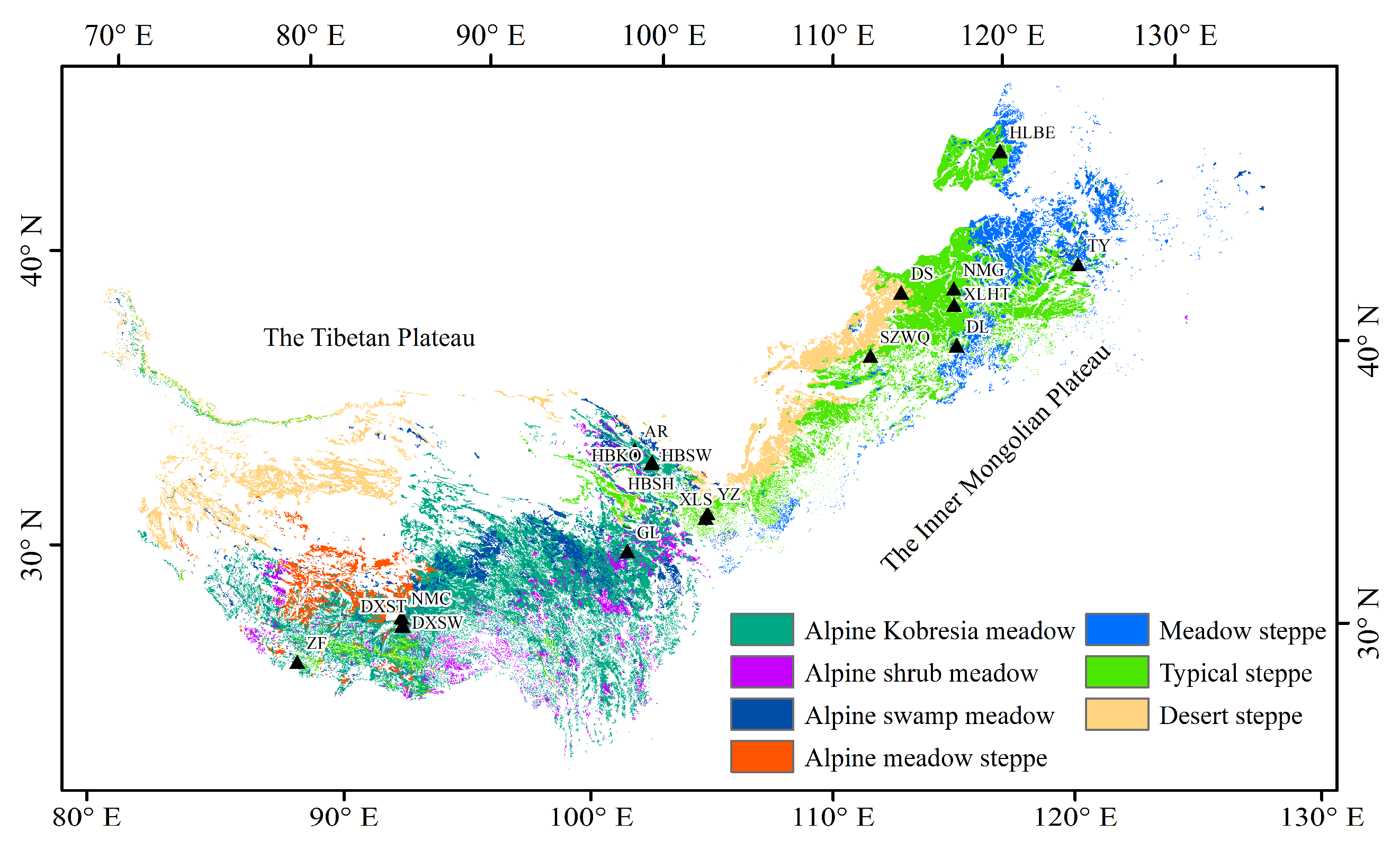
2.1. Study Area

Located in an alpine climate zone, the TP is characterized by lengthy sunshine duration, strong solar radiation, low temperature, and low precipitation (PRE). The average altitude of the TP is more than 4000 m, the mean annual air temperature is in the range of −5.75 to 2.57 °C, and the mean annual precipitation varies from 200 to 600 mm. The terrain of the TP slopes from northwest to southeast. Alpine grasslands cover more than 60% of the surface of the TP and are a unique grassland ecosystem among the world’s alpine regions [12]. IM is in an arid and semi-arid zone, and the average altitude is approximately 1000 m, with a terrain that is high in the south and low in the north. The mean annual air temperature in the IM ranges between 3 and 6 °C, and the mean annual precipitation ranges from 200 to 350 mm. Temperate grasslands are the main grassland type in the IM, and are a typical vegetation type (VT) in a temperate continental climate.
According to the Atlas of Grassland Resources of China (1:1,000,000) [50], alpine grasslands are divided into four subcategories, namely alpine Kobresia meadow (KO), alpine shrub meadow (SH), alpine swamp meadow (SW), and alpine meadow steppe (AS). Temperate grasslands are divided into three subcategories, namely meadow steppe (MS), typical steppe (TS), and desert steppe (DS) (Figure 1).

2.2. Data

2.2.1. Flux and Meteorological Data

Flux and meteorological data were collected from the ChinaFLUX [51], Coordinated Observations and Integrated Research over Arid and Semi-arid China (COIRAS) [52], and the Heihe Watershed Allied Telemetry Experimental Research (HiWATER) [53]. A total of 52 site-year observation data points collected from 18 flux sites during 2003–2014 were used in this study (Figure 1, Table 1). Among them, nine sites were distributed in the TP alpine grasslands and included 34 site-year observation data points. Another nine sites were distributed in the IM temperate grasslands and included 18 site-year observation data points. These flux sites represent the most extensive grassland ecosystem types, with a wide range of spatial, ecological, and climatic conditions.
The carbon flux data were processed through triple coordinate rotation, the Webb–Pearman–Leuning (WPL) correction, and abnormal data rejection [51]. To match the eight-day compositing interval of the MODIS products, the half-hour observed RE, Ta and photosynthetically active radiation (PAR) data were averaged and the PRE was summed over eight days. At the site scale, these meteorological data were synchronously observed using the eddy covariance system, and were gap-filled following the method proposed by Schwalm et al. [54]. Finally, we obtained a total of 1923 items of site observation data with an eight-day temporal resolution. At the wider spatial scale, Ta, PRE, and PAR data from 2001 to 2015 with 1 km spatial resolution were produced using ANUSPLIN software to spatialize the observation data from Chinese meteorological stations. The regional-scale Ta, PRE, and PAR data were then cross-validated based on the site observation data. The validation results showed that the interpolation products were consistent with the site observation data [55,56]. In line with the RE data, the regional Ta and PAR data were averaged and the PRE was summed for eight days.

2.2.2. Remote Sensing Data

According to Equation (1), the EVI was generated using the eight-day MODIS land surface reflectance datasets (MOD09A1, Level 3, Collection 5) for 2001–2015, which were downloaded from the NASA Land Processes Distributed Active Archive Center (https://lpdaac.usgs.gov/, accessed on 12 October 2021).
E V I = G ρ N I R ρ r e d ρ N I R + C 1 × ρ r e d C 2 × ρ b l u e + L
where ρ N I R , ρ r e d and ρ b l u e are the surface reflectance for the near-infrared, red, and blue bands, respectively. The coefficients G , C 1 , C 2 and L used in the EVI algorithm were 2.5, 6, 7.5, and 1, respectively [57].
The original spatial resolution of the EVI was 500 m; it was resampled to 1 km for ease of computation. To further reduce the effects of cloud and to capture the seasonality of the EVI, a data smoothing tool providing a double logistic curve fit in the TIMESAT software was used to smooth the original time series [58].
Digital elevation model (DEM) data was obtained from the Shuttle Radar Topographic Mission (https://srtm.csi.cgiar.org/srtmdata/, accessed on 10 November 2021) and the original data were resampled with a spatial resolution of 90 m to 1 km.

2.2.3. Soil Data

The SoilTex of the surface soil layer (0–30 cm) was retrieved from the Harmonized World Soil Database (http://webarchive.iiasa.ac.at/Research/LUC/External-World-soil-database/, accessed on 16 November 2021), including the clay content (wt%), silt content (wt%), and sand content (wt%). The soil organic carbon density (SOCD, kg C m−2) was calculated using the organic carbon content (wt%), gravel content (vol%), layer thickness (m), and bulk density (kg m−3), according to the method described by Carvalhais et al. [59]. Due to limited data availability, we only obtained one issue of SOCD and SoilTex data. We used the mean values of the SoilTex, SOCD, and EVI subsets of 3 × 3 km pixels centered on each flux tower, to better represent the eddy covariance footprint area and to reduce the effects of geolocation errors [34].

2.3. Model

2.3.1. Deep Learning Model: Geoman

In this study, we used a deep learning model including a multi-level attention mechanism, known as Geoman. It was originally developed to perform geographic sensor time-series predictions, such as for air quality and water quality [44]. The structure was modified from the original Geoman framework and is shown in Figure 2. Geoman combines the advantages of the attention mechanism and LSTM by distinguishing the importance of multiple time-series data to preserve key spatiotemporal information. The attention module in Geoman consists of spatial and temporal attention. The spatial attention includes two sub-modules, namely global spatial attention that expresses the inter-site correlations, and local spatial attention that expresses the intra-site correlations. The temporal attention in the decoder stage captures the time dependencies. LSTM learns interactions at multiple timescales and can be extended to encoder and decoder modules [60]. Limited by the availability of ecological data, and also by differences in the spatial density between ecological observation sites and other geographic monitoring sites, including loop detector systems and urban groundwater monitoring systems, we only used local spatial attention to describe the dynamic correlation between each local feature and the target series. For simplicity, in this paper the term ‘Geoman’ refers to the model without global spatial attention. The local spatial attention mechanism can be expressed simply by Equations (2) and (3).
e t k = v l T t a n h   W l   h t 1 ; s t 1 + U l   x k + b l
α t k = exp e t k j = 1 N l exp e t j
where ; represents concentration operation. v l , b l T , W l T × 2 m and U l T × T are learnable parameters and are determined by the back-propagation algorithm during the training process. The superscript T is the time window of input data. h t 1 m and s t 1 m are the hidden state and cell state at time t 1 , constituting the short-term memory and long-term memory in the LSTM encoder, respectively. The superscript m is the number of hidden neurons in LSTM. N l denotes the number of feature variables. x k is the k-th local feature, namely the environmental variables (VT, Ta, PAR, EVI, PRE, SOCD, or SoilTex) of the flux sites. e t k is the correlation score between the k-th local feature and the target series (i.e., RE). Its size is determined by the local input feature x k and historical state information ( h t 1 and s t 1 ). α t k is the attention weight calculated by normalizing the score of the k-th feature using a softmax function, and represents the relative importance of the k-th feature to the target series. After training, α t k was obtained from the trained Geoman prediction process. The external factor fusion module can fuse other relevant features affecting the RE, such as elevation and weather forecasts. The weather forecasts used in this study refer to Ta and PRE at the time stamp of the predicted RE, and provide time-related factors to further improve the prediction accuracy.

2.3.2. Model Training and Evaluation

The hyperparameters of Geoman were optimized and determined using the grid search method [61]. All data from the 18 sites were fed into the model for training, without considering the interactions between sites. The performance of Geoman was evaluated using a sample-based 10-fold cross-validation strategy in which the observation data were randomly assigned 10 folds. Each fold contained approximately 10% of the data and was used consecutively for model training, validation, and testing to ensure independence of the three datasets [60]. According to this partition principle, the entire data were divided into non-overlapping training, validation, and test data at a ratio of 8:1:1. The cross-validation process was repeated 10 times. The estimated RE from all 10 folds were compared with the observed RE.
Three frequently used statistical indicators, i.e., the coefficient of determination (R2), root-mean-square error (RMSE), and mean absolute error (MAE) were selected as evaluation metrics to analyze the performance of the model. These metrics were calculated as follows:
R 2 = i = 1 n y i y ¯ y i y ¯ i = 1 n y i y ¯ 2 i = 1 n y i y ¯ 2 2
R M S E = 1 n i = 1 n y i y i 2
M A E = 1 n i = 1 n y i y i
where y i and y i are the observed and estimated RE, respectively. y ¯ and y ¯ are the means of y i and y i , and n is the number of observed samples.
When all parameters were optimized, the trained Geoman model was applied to predict eight-day RE at all spatial grids, using environmental data with l km spatial resolution and eight-day temporal resolution. The grid numbers for each grassland subtype are shown in Table 2. The DEM, SOCD, and SoilTex data were set unchanged at all time steps due to their limited availability.

3. Results

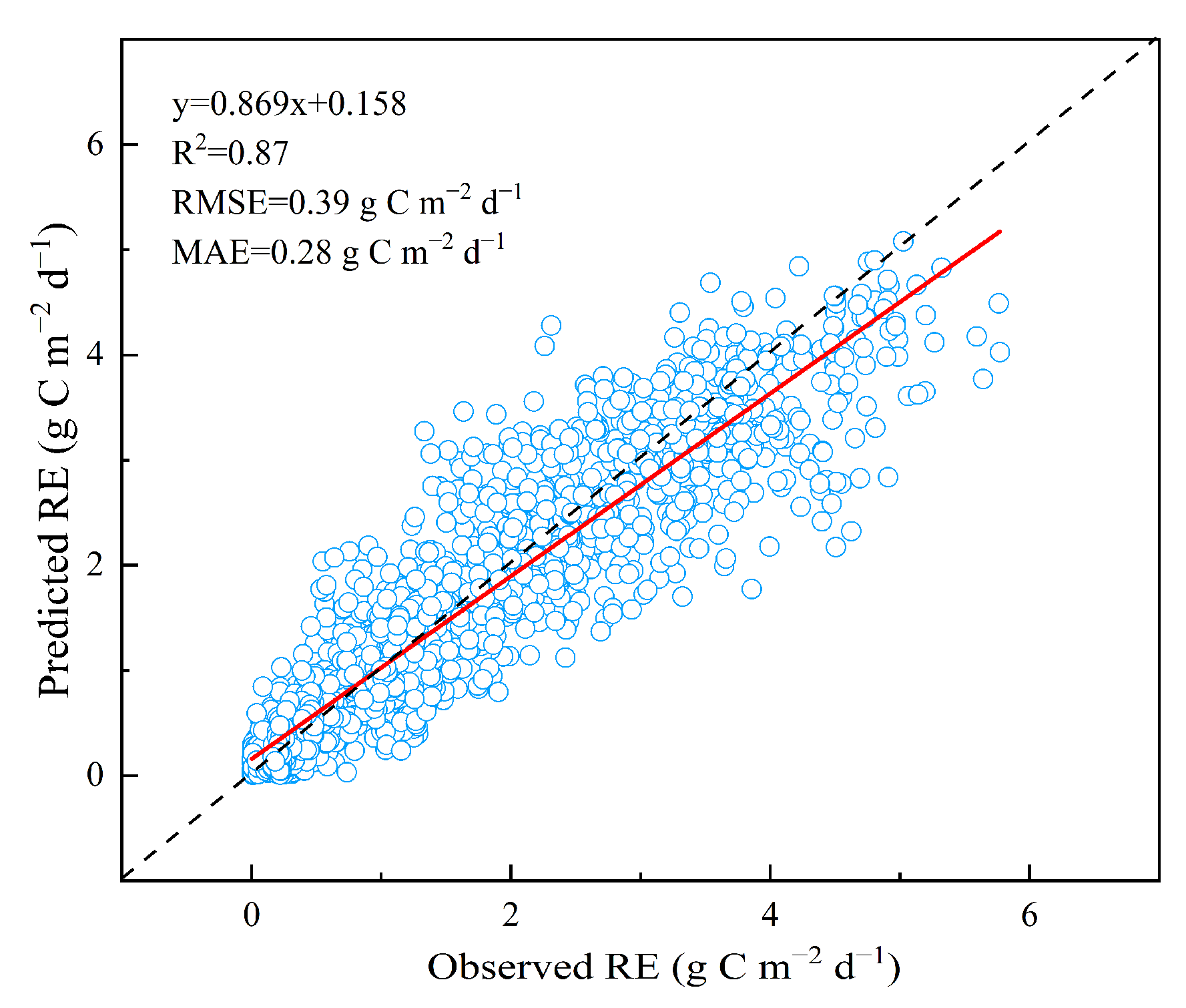
3.1. The Performance of Geoman at the Site Scale

3.1.1. Model Evaluation

According to the results of the 10-fold cross-validation, the predicted RE was in line with the observed RE (Figure 3). Most of the scattered points occurred approximately at the 1:1 line (R2 = 0.87, RMSE = 0.39 g C m−2 d−1, MAE = 0.28 g C m−2 d−1), indicating that Geoman can accurately estimate the RE value for northern China’s grasslands.
We further evaluated the model simulation for the seasonal dynamics of RE at the site scale. Results showed that Geoman can accurately capture the seasonal dynamics of RE in the seven grassland subtypes (Figure S1). The best agreement between the predicted and observed RE was for typical steppe and meadow steppe (R2 = 0.97 and 0.95, respectively), followed by the alpine shrub meadow (R2 = 0.91), alpine Kobresia meadow (R2 = 0.89), desert steppe (R2 = 0.88), alpine swamp meadow (R2 = 0.86), and alpine meadow steppe (R2 = 0.86).
The seasonal variation in the RE at all sites formed a unimodal curve, peaking in July or August. The model continued to perform well during the high value period (from July to August), the growing season (from May to September), and the low value period (from December to January) in the non-growing season. Across the seven grassland subtypes, the alpine Kobresia meadow, the alpine shrub meadow, and the meadow steppe had higher RE peaks, reaching 4–6 g C m−2 d−1 (Figure S1a,b,f), while the alpine meadow steppe and desert steppe had relatively low RE peaks of 0.5–2 g C m−2 d−1 (Figure S1d,f).

3.1.2. Relative Importance of Environmental Factors

In this study, we quantified the relative importance of each environmental variable for predicting the RE, using the dynamic attention weights. We analyzed the differences between seven grassland subtypes during the growing season and non-growing season (Figure 4, Table 3). Results demonstrate that vegetation type and soil texture are the two most important environmental factors for RE estimation in northern China’s grasslands. The importance of other environmental variables also represents spatiotemporal characteristics with ecological significance. In the growing season, temperature was found to be more important than precipitation in alpine grasslands, whereas the opposite was true for temperate grasslands. This indicates that restrictive climatic conditions have a considerable effect on accurate estimation of RE. In the non-growing season, SOCD was more important than climatic variables for RE estimation. However, temperature was more important than SOCD in alpine meadows, which may be associated with the low temperature limit of the RE in the area.
Evaluation of the relative importance of the environmental variables indicates that the importance of SOCD in the non-growing season exceeded that of the climatic factors. Therefore, we further evaluated the accuracy of the RE estimation for the low value period from December to January in the non-growing season. It was found that adding SOCD to the model could improve interpretability by 44% compared with removing this variable (Figure S2a,b). When the soil texture was removed from the model, the results appeared to have been overestimated during the low value period in the non-growing season (Figure S2c). Therefore, it is necessary to integrate soil texture into RE models because this can to a certain extent solve the problem of overestimation of low RE values.

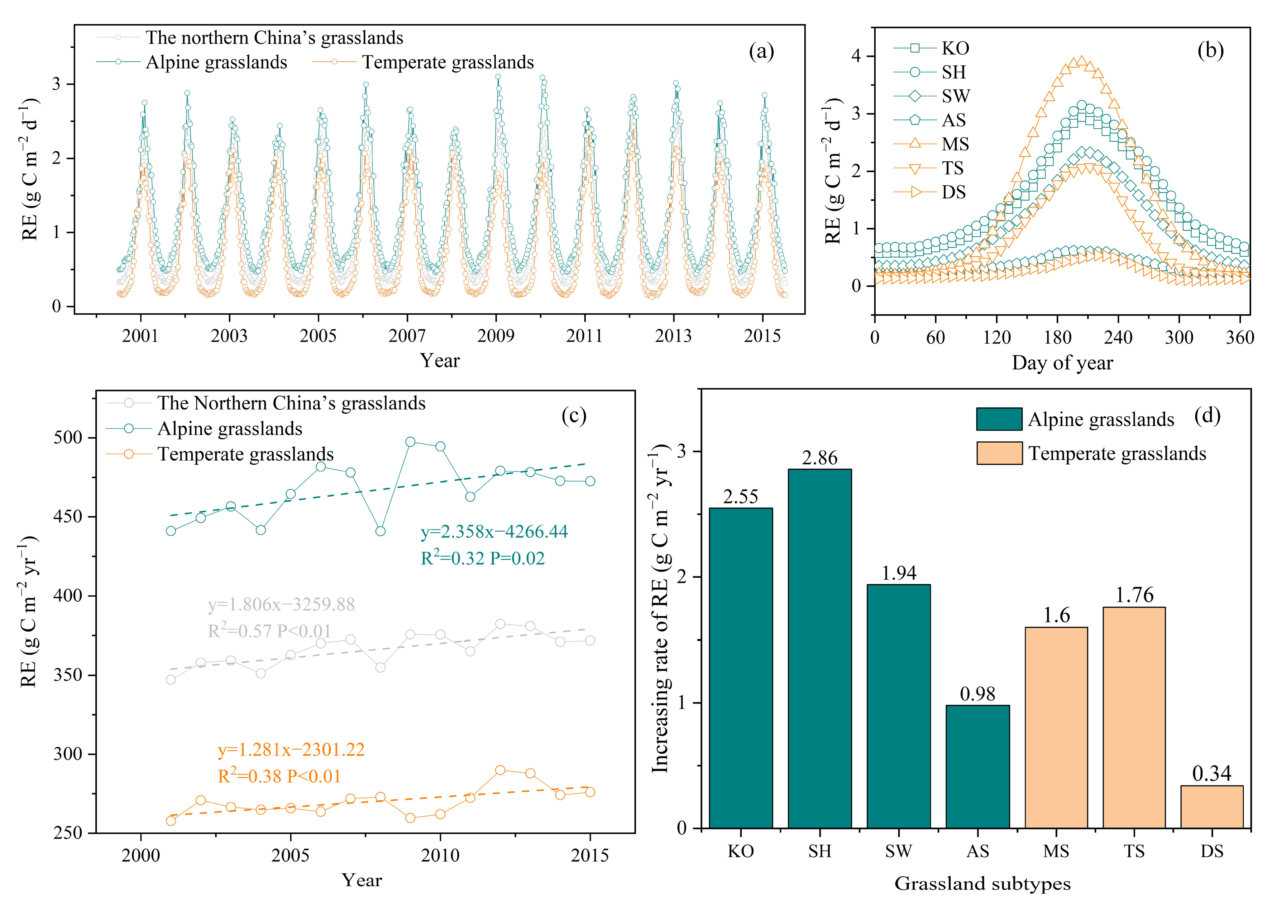
3.2. Spatiotemporal Changes in RE in Northern China’s Grasslands

3.2.1. Spatial Patterns of RE in Northern China’s Grasslands

The mean annual RE for northern China’s grasslands from 2001 to 2015 was 366.53 g C m−2 yr−1, showing clear spatial heterogeneity. However, the spatial patterns for RE over the 15 years did not change significantly (Figure 5a). Regarding the alpine grasslands on the TP, the mean annual RE was 467.44 g C m−2 yr−1, exhibiting a clear decreasing gradient from southeast to northwest (Figure 5b). The alpine shrub meadow had the largest RE (573.64 g C m−2 yr−1), followed by the alpine Kobresia meadow (515.28 g C m−2 yr−1), the alpine swamp meadow (380.94 g C m−2 yr−1), and the alpine meadow steppe (129.29 g C m−2 yr−1). Regarding the temperate grasslands in IM, the mean annual RE was 270.43 g C m−2 yr−1, exhibiting a clear decreasing gradient from northeast to southwest (Figure 5b). The highest RE value occurred in the meadow steppe (534.28 g C m−2 yr−1) in the northeast, and the lowest value for RE was recorded in the desert steppe in the southwest (88.15 g C m−2 yr−1). The mean annual RE in the typical steppe was 283.15 g C m−2 yr−1. Statistics indicated that the RE for the alpine Kobresia meadow and typical steppe accounted for more than 60% of the total RE in northern China’s grasslands (Figure 5c).

3.2.2. Temporal Variation for RE in Northern China’s Grasslands

Seasonal variation in RE at the regional scale formed a unimodal curve peaking during summer (Figure 6a), which is consistent with the site-scale verification results (Figure S1). The RE for alpine grasslands in the TP was always higher than that of the temperate grasslands in the IM. The RE peak value for the TP was in the range of 2.5–3.0 g C m−2 day−1, and its trough value was around 0.5 g C m−2 day−1. The IM had a lower peak value of 2.0–2.5 g C m−2 day−1, and its trough value was significantly lower than 0.5 g C m−2 day−1. We analyzed seasonal dynamics for the mean 15-year seasonal RE in the seven grassland subtypes and found that vegetation heterogeneity had a significant impact on RE (Figure 6b). The seasonal change curves for RE in the alpine meadow steppe and desert steppe were relatively flat, and the differences in RE between the growing season and non-growing season were relatively small, which may have resulted from hydrothermal condition limitations. Compared with these two grassland subtypes, the other grassland subtypes had a higher RE peak value during the growing season.
From 2001 to 2015, the RE of northern China’s grasslands increased at a rate of 1.81 g C m−2 yr−1 (Figure 6c). The alpine grassland RE in TP increased at a rate of 2.36 g C m−2 yr−1, which was faster than the increase rate of 1.28 g C m−2 yr−1 in the IM temperate grasslands (Figure 6c). We further analyzed the increase rate of RE in the seven grassland subtypes from 2001 to 2015 and found that the maximum rate of increase occurred in the alpine shrub meadow, while the minimum increase rate was in the desert steppe (Figure 6d). The rate of increase for RE in the TP is greater than that of the IM, which shows that the TP has a stronger feedback response under the background of global climate change.

3.3. Environmental Effects on RE Spatiotemporal Variation

3.3.1. Environment Effects on RE Seasonal Dynamics

The relationship between RE and Ta in northern China’s grasslands at an eight-day timescale showed an explicit exponential form (R2 = 0.97; Figure 7a). The sensitivity of RE to temperature in the TP alpine region was greater than that of the IM temperate region. This temperature-sensitive heterogeneity can be attributed to the regional climatic conditions and the vegetation types. There was a clear positive correlation between RE and PRE throughout northern China’s grasslands, and the R2 between the two was 0.90 (Figure 7b). We also found that the RE reached a certain saturation point with the increase in PRE. When the PRE reacheds a specific threshold, the RE no longer increased and even tended to decline (Figure 7b). The saturation thresholds for RE to PRE differed in different climatic regions. In the temperate grasslands, RE began to decrease after the PRE exceeded 35 mm, while PRE at this intensity retained a continuous positive stimulus for RE in alpine grasslands. This may be associated with the different moisture requirements of the different grassland types. A significant linear positive correlation (R2 = 0.93) between the RE and the EVI was observed in the northern grasslands of China (Figure 7c). Similar to Ta, PAR and RE showed an exponential positive correlation (R2 = 0.69, Figure 7d). However, under the same radiation intensity, the sensitivity of RE to PAR was higher in the alpine grasslands than in the temperate grasslands.
We further analyzed the relationship between RE and environmental variables on a seasonal scale in the seven grassland subtypes (Table 4). It was found that Ta could best explain the RE seasonal dynamics compared with other variables, in five of the seven grassland subtypes. Ta was also the secondary environmental factor explaining the RE seasonal dynamics in the remaining two grassland subtypes. To summarize, Ta was found to dominate the seasonal dynamics of RE in northern China’s grasslands.

3.3.2. Environment Effects on RE Interannual Dynamics

With respect to each grassland type, we analyzed the interannual dynamic relationship between RE and environmental variables (Figure 8, Table 5). In the four alpine grassland subtypes, the R2 between the annual RE and annual average Ta was 0.73–0.91 (Figure 8a). The R2 between the annual RE and annual average EVI, excluding the alpine meadow steppe, was 0.44–0.63 (Figure 8c). There was no significant correlation between the annual RE and the annual total PRE or PAR (Figure 8b,d). In the three temperate grassland subtypes, the R2 between the annual RE and the annual total PRE was 0.2–0.64 (Figure 8b). The R2 between the annual RE and the annual average EVI was 0.28–0.63 (Figure 8c), but there was no significant correlation with the annual average Ta or the annual PAR (Figure 8a,d). In contrast to the positive promotion effect of PAR on RE at the seasonal scale (Figure 7d), the effect of annual total PAR on annual RE was not significant (Figure 8d).
We found that when the mean annual PRE exceeded 400 mm, which was the case in all the alpine grasslands and in MS among the temperate grasslands (Table 5), annual average Ta always provided a positive stimulus for annual RE (Figure 8a). This suggests that in grasslands with adequate moisture availability, the interannual dynamics of RE were controlled by factors other than PRE. Compared with the significant positive correlation between annual average RE and annual total PRE in temperate grasslands, the correlation for these in alpine grasslands was negative or close to zero (Figure 8b). When temperature was restricted, the annual total PRE had almost no stimulating effect on the annual RE in the same grassland type. In summary, the interannual change in RE in alpine grassland is mainly attributed to the annual average Ta and annual average EVI, and the interannual change in RE in temperate grassland is attributed to the annual total PRE and annual average EVI.

3.3.3. Environment Effects on RE Spatial Variation

The red fitting line in Figure 8 shows that annual RE was correlated with the annual average EVI across the seven grassland subtypes, and the R2 reached 0.91. This indicates that EVI can best explain the spatial variation in RE in northern China’s grasslands, compared with other environmental factors. In alpine grasslands, including AS, SW, KO, and SH, the mean 15-year EVI showed an increasing trend, and RE also showed an increasing trend (Figure 8c, Table 5). In temperate grasslands, EVI and RE also increased simultaneously from DS and TS to MS. These results highlight that RE and EVI changed synchronously in the same spatial direction in the same climate zone.
In the temperate grasslands, including DS, TS, and MS, the mean annual RE increased synchronously with an increase in the mean annual PRE (Figure 8b). Within AS, SW, KO, and SH in the alpine grasslands, the mean annual PRE and the mean annual RE also increased simultaneously. However, simultaneous variation in the PRE and the RE was only observed in the same climate zone. Across grassland types in the same climate zone, the mean annual PRE controlled the magnitude of the mean annual RE.
There was no significant correlation (R2 = 0.004, p = 0.52) between annual RE and annual average Ta throughout northern China’s grasslands (Figure 8a). In the alpine grasslands, including AS, SW, KO, and SH, the annual RE increased with an increase in the annual average Ta. However, in the temperate grasslands, there no synchronization phenomenon was observed. These results indicate that the dependence of annual RE on the annual average Ta tends to be stronger in regions with more moisture. The influence of Ta on RE in grassland ecosystems is regulated by moisture, and the regulation strength varies with different vegetation types.
Across the seven grassland subtypes, the SOCD, clay, and silt content had positive effects on the mean annual RE, whereas sand content had a negative effect (Figure 9), which is consistent with previous research [27]. Within AS, SW, KO, and SH in the alpine grasslands and DS, TS and MS in the temperate grasslands, RE increased simultaneously with the increase in SOCD and clay content. The R2 between the RE and the SOCD, clay, silt, and sand content were 0.80, 0.68, 0.45, and 0.81, respectively, implying that soil factors also affect the spatial variation of RE.
EVI and soil factors are critical environmental factors that determine the spatial variations in RE in northern China’s grasslands. Their dominant roles illustrate the importance of grassland type and soil factors in regulating the spatial pattern of RE.

4. Discussion

4.1. Model Comparison

Accuracy comparison between Geoman and the previous models in estimating RE in northern China’s grasslands is displayed in Table 6. Geoman performed best, with the best explanation and minimum bias, when compared with seven previous models, including two semi-empirical models, one satellite-based model, three traditional machine-learning models, and one deep-learning model. Compared with semi-empirical models, deep-learning models can automatically extract the complex nonlinear dependence relationship between the target variable and the explaining variable, without excessive restriction from predetermined theoretical assumptions about complicated respiration processes. Based on similar methods, carbon flux estimations such as gross primary productivity (GPP) have been used as benchmarks and are widely employed in the evaluation and improvement of process models [62,63,64]. The combination of LSTM and the attention mechanism in the encoder and decoder stages further improves the predictive ability of the Geoman model (see Section 3.1.1). The LSTM in Geoman can adapt to time-varying behaviors and use dynamic data to update the parameters to improve the predictions. The local spatial attention module provides a means of distinguishing the importance of different input variables. The time attention module gains insight into past patterns of encoder outputs for different environment variables, and decoder outputs for the target variables. However, this insight can be difficult to model using traditional ML models.
Despite the many challenges in adopting DL in ecology, DL can provide predictions with unparalleled precision without prior hypotheses. Geoman has been designed to make time-series predictions by understanding the impact of multiple explanatory variables on the target variables. However, the interpretation of the prediction results from the DL model structure is often insufficient, because the impact of the inputs on the outputs cannot be easily understood through neural networks [30]. In this study, an attempt was made to use the attention mechanism to explain the impact of environmental variables on RE, ecologically meaningful results were generated (see Section 3.1.2). The integration of DL models and ecological-process-based models represents a promising development in the domain of ecological study, and should substantially improve the interpretability of the DL models [65].

4.2. Climatic and Biotic Control over RE

Climatic conditions regulate the spatiotemporal patterns and variation in RE [1,66]. Temperature is the main factor affecting the RE rate in the absence of other environmental stresses [67]. This is because respiration requires the catalysis of enzymes, and temperature is a necessary condition for enzyme decomposition [68]. According to our results (see Section 3.3.2), warming promoted an increase in RE in alpine grasslands across the four alpine grassland subtypes as well as within the same subtype. It did not lead to an increase in RE in temperate grasslands, and even led to a decrease in RE in TS and DS (Figure 8a). Warming had no effect on RE, which may be related to the limited precipitation in temperate grasslands (Figure S3b) that restricts plant production and microbial activity [69]. This also indicates that warming can increase the RE under favorable environmental conditions when moisture availability is not a restrictive factor.
PRE provides the necessary water for vegetation growth, affecting canopy structure and plant production [70], and ultimately improves autotrophic respiration. PRE changes the soil microenvironment, affecting the dissolution and diffusion of organic solutes, gases, and enzymes [67,71]. This promotes microbial activity [72], and improves heterotrophic respiration. However, a saturation phenomenon affects RE under conditions of high precipitation (Figure 7b), which has been reported in previous studies [13,27]. This may be because precipitation in excess of the saturated soil moisture reduces the oxygen content in the soil [27,68]. It also inhibits the activity of plant roots and aerobic microorganisms, and reduces RE in grasslands. The different levels of saturated PRE for RE in alpine grasslands and temperate grasslands may reflect differences in the water requirements for different vegetation types.
The increase in the annual total PRE, and not the annual average Ta, had a positive effect on the annual RE within the same temperate grassland subtype (Figure 8a,b). This may be associated with the greater increase in precipitation than in temperature from 2001–2015 (Figure S3a,b). The annual average Ta had a greater stimulating effect on the increase in annual RE in the same alpine grassland subtype (Figure 8a), which was associated with the increase in the annual average Ta (Figure S3a). These results illustrate that PRE and Ta were the dominant climatic factors for interannual changes in RE in temperate grasslands and alpine grasslands, respectively. IM temperate grasslands are mainly distributed in arid and semi-arid zones, and limited moisture strongly restricts vegetation growth and microbial activity, which each affect RE changes [34]. Although plants that grow in alpine regions have adapted to the low temperature environment, their production and respiration processes are comparatively restricted. A minor temperature rise can contribute to an increase in RE by prompting the grassland to turn green, and increasing the biomass, the microbial activity, and litter decomposition [73,74,75].
The promoting effect of PAR on RE at the seasonal scale can be attributed to the effect of the seasonal PAR cycle on photosynthesis. Stronger photosynthesis tends to mean stronger respiration. However, at the interannual scale, the influence of annual PAR on annual RE changes was not significant in the alpine grasslands nor in the temperate grasslands (Figure 8d), which may be related to the long-term stability of solar radiation (Figure S3d).
This study indicates that EVI is the most important environmental factor affecting the spatial pattern of RE in northern China’s grasslands (Figure 8c), which is in accordance with previously reported results [12,16]. As a vegetation index commonly used for estimation of vegetation productivity, EVI is strongly associated with GPP in space and time [76,77]. GPP is the main supply for autotrophic respiration, and determines its intensity [24]. Decomposition of organic matter by microorganisms, including heterotrophic soil respiration, is also supported by photosynthesis. As shown in Figure S3c, the rate of increase for EVI in temperate grasslands from 2001 to 2015 was substantially greater than that in the alpine grasslands. This illustrates the faster increase in productivity of temperate grasslands, although the rate of increase for RE in temperate grasslands over 15 years was slower than that in the alpine grasslands (Figure 6c). This may be due to the greater uptrend of carbon sequestration in temperate grasslands [78].
The soil carbon substrate supplies various components of the RE, and determines the distribution of nutrients in aboveground and underground plant tissues, as well as the phenological patterns of vegetation growth [67]. Soil organic carbon (SOC) is one of the main forms of soil carbon that affects spatiotemporal patterns of respiration [1,79]. With a relatively large soil carbon pool and gradually melting permafrost, alpine grasslands on the TP have the potential to release significant amounts of CO2 [80]. Our results also demonstrate that the RE and its rate of increase on the TP are larger than those in the IM (Figure 6c). SoilTex indirectly influences RE, primarily by controlling water and nutrient availability [81,82]. Clay and silt soils have higher soil water-holding capacities and longer water-holding times [83]. This provides more available water for vegetation growth, microbial decomposition, and respiration. Soils with higher clay and silt content can also store more SOC and nutrients for respiration processes [14,27]. The negative impacts of sand content on respiration could be attributed to larger soil porosity, resulting in lower soil water availability. This may constrain microbial activity and vegetation growth, leading to reduced respiration.
The effects of biotic and climatic factors on RE are strongly interlinked. Adequate hydrothermal conditions increase vegetation growth and autotrophic respiration [84]. These hydrothermal and vegetation conditions further regulate the SOC and affect the soil heterotrophic respiration [85]. Biotic and climatic factors synergistically stimulate RE, but at different spatial and temporal scales, and one of these variables may be particularly significant.

4.3. Limitations and Prospects

The carbon, water, and energy flux estimations for the regional scale based on the ML models represent a process of upscaling ecological knowledge of the carbon cycle from the site scale. Therefore, it is essential to evaluate the spatial representativeness of the flux observation sites [86,87]. Most of the current flux observation sites were established gradually over the previous few decades, with their locations often having been determined by expert experience and consideration of accessibility, including traffic, logistics, and topographic factors. Site density and uniformity substantially vary in different regions, owing to the lack of a systematic design. The 18 flux sites used in this study exhibited a non-uniform spatial distribution (Figure 1). In situ observations representing a few surrounding kilometers cannot fully represent the climate, environment, and flux in remote regions [88]. This increases the level of uncertainty in regional-scale carbon-flux estimations [89,90]. It has been reported that the current network of flux towers in northwestern Tibet lacks representativeness, and that adding flux towers could considerably improve the ability of the existing flux network to represent local environmental conditions [91]. It is expected that the ecological environment will receive more public attention, and the rapid expansion of big data in ecological systems engineering will establish an increasing number of flux sites, so their representativeness will become more credible.
The time range of carbon flux data employed in this study was concentrated in the period 2003–2014 (Table 1). This approximately coincides with the long-term regional estimation of RE. However, we obtained only one-year flux data for the AR, NMC, ZF, HLBE, SZWQ, and XLS sites. The small amount of observation data not only means these sites were under-represented, but may also make it impossible for the Geoman model to learn adequately the features of these flux data during model training. The estimated RE in this study is based on time-series environmental data with an eight-day resolution. These environmental variables cannot fully reflect various extreme climatic events that occurred during the eight-day interval [92], such as extreme heat waves or rainfall in summer and extreme cold in winter. The limited availability and considerable uncertainty of SOC and soil texture data restrict their effective application in estimating the RE at the regional scale [17,59,93]. The continuous sharing of ecological data, and the development of data augmentation and digital soil mapping technologies will provide reliable solutions to these problems.

5. Conclusions

Compared with several previous semi-empirical models and traditional ML models, Geoman performed better (R2 = 0.87, RMSE = 0.39 g C m−2 yr−1, MAE = 0.28 g C m−2 d−1) when estimating RE in northern China’s grasslands. We found that soil factors have a significant effect on the estimation of RE in the low-value period in the non-growing season, thereby suggesting that RE models should not exclude the role of soil, especially in grassland ecosystems. Our results revealed the occurrence of substantial spatiotemporal changes in RE in northern China’s grasslands. On the spatial scale, the RE of alpine grassland showed a decreasing trend from southeast to northwest in the TP, and that of temperate grassland showed a decreasing trend from northeast to southwest in the IM. On the temporal scale, the RE of grasslands in northern China showed a significant increasing trend (1.81 g C m−2 yr−1) from 2001 to 2015. The rapid increase in RE in alpine grasslands indicates greater response to climate change than in temperate grasslands. Biotic and climatic control over RE varied at the temporal and spatial scales. Ta was the main factor that influenced the seasonal dynamics of RE in grassland ecosystems. Ta and EVI controlled the interannual dynamics of RE in alpine grasslands, whereas PRE and EVI were the main controlling factors in temperate grasslands. EVI and soil factors were found to control the spatial changes in RE in grassland ecosystems. This study highlights the high accuracy of DL in simulating spatiotemporal changes in the carbon cycle, and enhances our understanding of the interactions between RE and climate change.

Supplementary Materials

The following supporting information can be downloaded at: https://0-www-mdpi-com.brum.beds.ac.uk/article/10.3390/rs14153563/s1, Figure S1: Eight-day time series plots for observed and predicted RE at all sites; Figure S2: Predicted RE vs. observed RE in the low value period in the non-growing season; Figure S3: Interannual dynamics of annual average Ta, annual total PRE, annual average EVI, and annual total PAR from 2001–2015 at the regional scale.

Author Contributions

Conceptualization, W.L. and H.H.; methodology, W.L. and X.W.; software, W.L.; validation, W.L, X.R. and L.Z.; formal analysis, X.Z.; data curation, L.F. and Y.L.; writing—original draft preparation, W.L.; writing—review and editing, H.H. and X.W.; visualization, Q.C. and Q.X.; supervision, M.Z.; project administration, Y.Z. and T.W.; funding acquisition, H.H. All authors have read and agreed to the published version of the manuscript.

Funding

This research was funded by the National Natural Science Foundation of China (the Study on Carbon Sequestration Rate and Its Uncertainty, Stability and Sustainability of Terrestrial Ecosystems in China, No. 42141005).

Data Availability Statement

All data can be accessed through the provided website and references.

Acknowledgments

We thank the staff of ChinaFLUX, COIRAS and HiWATER for their dedication in observation and data processing. We also thank Qinmeng Yang (Computer Network Information Center, Chinese Academy of Sciences) for his guidance.

Conflicts of Interest

The authors declare no conflict of interest.

References

  1. Migliavacca, M.; Reichstein, M.; Richardson, A.D.; Colombo, R.; Sutton, M.A.; Lasslop, G.; Tomelleri, E.; Wohlfahrt, G.; Carvalhais, N.; Cescatti, A.; et al. Semiempirical modeling of abiotic and biotic factors controlling ecosystem respiration across eddy covariance sites. Glob. Change Biol. 2011, 17, 390–409. [Google Scholar] [CrossRef]
  2. Tang, X.; Zhou, Y.; Li, H.; Yao, L.; Ding, Z.; Ma, M.; Yu, P. Remotely monitoring ecosystem respiration from various grasslands along a large-scale east–west transect across northern China. Carbon Balance Manag. 2020, 15, 6. [Google Scholar] [CrossRef] [PubMed]
  3. Luo, Y.Q. Terrestrial carbon-cycle feedback to climate warming. Annu. Rev. Ecol. Evol. Syst. 2007, 38, 683–712. [Google Scholar] [CrossRef] [Green Version]
  4. Wohlfahrt, G.; Anderson-Dunn, M.; Bahn, M.; Balzarolo, M.; Berninger, F.; Campbell, C.; Carrara, A.; Cescatti, A.; Christensen, T.; Dore, S.; et al. Biotic, Abiotic, and Management Controls on the Net Ecosystem CO2 Exchange of European Mountain Grassland Ecosystems. Ecosystems 2008, 11, 1338–1351. [Google Scholar] [CrossRef]
  5. Zheng, C.; Tang, X.; Gu, Q.; Wang, T.; Wei, J.; Song, L.; Ma, M. Climatic anomaly and its impact on vegetation phenology, carbon sequestration and water-use efficiency at a humid temperate forest. J. Hydrol. 2018, 565, 150–159. [Google Scholar] [CrossRef]
  6. Jung, M.; Reichstein, M.; Margolis, H.A.; Cescatti, A.; Richardson, A.D.; Altaf Arain, M.; Arneth, A.; Bernhofer, C.; Bonal, D.; Chen, J.; et al. Global patterns of land-atmosphere fluxes of carbon dioxide, latent heat, and sensible heat derived from eddy covariance, satellite, and meteorological observations. J. Geophys. Res. Biogeosci. 2011, 116, G3. [Google Scholar] [CrossRef] [Green Version]
  7. Ai, J.; Jia, G.; Epstein, H.E.; Wang, H.; Zhang, A.; Hu, Y. MODIS-Based Estimates of Global Terrestrial Ecosystem Respiration. J. Geophys. Res. Biogeosci. 2018, 123, 326–352. [Google Scholar] [CrossRef]
  8. Li, W.; Ciais, P.; Wang, Y.; Yin, Y.; Peng, S.; Zhu, Z.; Bastos, A.; Yue, C.; Ballantyne, A.P.; Broquet, G.; et al. Recent Changes in Global Photosynthesis and Terrestrial Ecosystem Respiration Constrained From Multiple Observations. Geophys. Res. Lett. 2018, 45, 1058–1068. [Google Scholar] [CrossRef]
  9. Niu, B.; Zhang, X.; Piao, S.; Janssens, I.A.; Fu, G.; He, Y.; Zhang, Y.; Shi, P.; Dai, E.; Yu, C.; et al. Warming homogenizes apparent temperature sensitivity of ecosystem respiration. Sci. Adv. 2021, 7, eabc7358. [Google Scholar] [CrossRef]
  10. Huang, N.; Wang, L.; Song, X.-P.; Black, T.A.; Jassal, R.S.; Myneni, R.B.; Wu, C.; Wang, L.; Song, W.; Ji, D.; et al. Spatial and temporal variations in global soil respiration and their relationships with climate and land cover. Sci. Adv. 2020, 6, eabb8508. [Google Scholar] [CrossRef]
  11. Bond-Lamberty, B. New Techniques and Data for Understanding the Global Soil Respiration Flux. Earth’s Future 2018, 6, 1176–1180. [Google Scholar] [CrossRef] [Green Version]
  12. Ge, R.; He, H.; Ren, X.; Zhang, L.; Li, P.; Zeng, N.; Yu, G.; Zhang, L.; Yu, S.-Y.; Zhang, F.; et al. A Satellite-Based Model for Simulating Ecosystem Respiration in the Tibetan and Inner Mongolian Grasslands. Remote Sens. 2018, 10, 149. [Google Scholar] [CrossRef] [Green Version]
  13. Wan, S.; Norby, R.J.; Ledford, J.; Weltzin, J.F. Responses of soil respiration to elevated CO2, air warming, and changing soil water availability in a model old-field grassland. Glob. Change Biol. 2007, 13, 2411–2424. [Google Scholar] [CrossRef]
  14. Reichstein, M.; Rey, A.; Freibauer, A.; Tenhunen, J.; Valentini, R.; Banza, J.; Casals, P.; Cheng, Y.; Grünzweig, J.M.; Irvine, J.; et al. Modeling temporal and large-scale spatial variability of soil respiration from soil water availability, temperature and vegetation productivity indices. Glob. Biogeochem. Cycles 2003, 17, 4. [Google Scholar] [CrossRef]
  15. McCulley, R.L.; Burke, I.C.; Nelson, J.A.; Lauenroth, W.K.; Knapp, A.K.; Kelly, E.F. Regional Patterns in Carbon Cycling Across the Great Plains of North America. Ecosystems 2005, 8, 106–121. [Google Scholar] [CrossRef]
  16. Jägermeyr, J.; Gerten, D.; Lucht, W.; Hostert, P.; Migliavacca, M.; Nemani, R. A high-resolution approach to estimating ecosystem respiration at continental scales using operational satellite data. Glob. Change Biol. 2014, 20, 1191–1210. [Google Scholar] [CrossRef]
  17. Luo, Y.; Ahlström, A.; Allison, S.D.; Batjes, N.H.; Brovkin, V.; Carvalhais, N.; Chappell, A.; Ciais, P.; Davidson, E.; Finzi, A.; et al. Toward more realistic projections of soil carbon dynamics by Earth system models. Glob. Biogeochem. Cycles 2016, 30, 40–56. [Google Scholar] [CrossRef]
  18. Yuan, W.; Luo, Y.; Li, X.; Liu, S.; Yu, G.; Zhou, T.; Bahn, M.; Black, A.; Desai, A.; Cescatti, A.; et al. Redefinition and global estimation of basal ecosystem respiration rate. Glob. Biogeochem. Cycles 2011, 25, 4. [Google Scholar] [CrossRef]
  19. Huang, N.; Niu, Z.; Zhan, Y.; Xu, S.; Tappert, M.C.; Wu, C.; Huang, W.; Gao, S.; Hou, X.; Cai, D. Relationships between soil respiration and photosynthesis-related spectral vegetation indices in two cropland ecosystems. Agric. For. Meteorol. 2012, 160, 80–89. [Google Scholar] [CrossRef]
  20. Lei, J.S.; Guo, X.; Zeng, Y.F.; Zhou, J.Z.; Gao, Q.; Yang, Y.F. Temporal changes in global soil respiration since 1987. Nat. Commun. 2021, 12, 403. [Google Scholar] [CrossRef]
  21. Dilustro, J.J.; Collins, B.; Duncan, L.; Crawford, C. Moisture and soil texture effects on soil CO2 efflux components in southeastern mixed pine forests. For. Ecol. Manag. 2005, 204, 87–97. [Google Scholar] [CrossRef]
  22. Lohila, A.; Aurela, M.; Regina, K.; Laurila, T. Soil and total ecosystem respiration in agricultural fields: Effect of soil and crop type. Plant Soil 2003, 251, 303–317. [Google Scholar] [CrossRef]
  23. Franzluebbers, K.; Franzluebbers, A.J.; Jawson, M.D. Environmental controls on soil and whole-ecosystem respiration from a tallgrass prairie. Soil Sci. Soc. Am. J. 2002, 66, 254–262. [Google Scholar]
  24. Janssens, I.A.; Lankreijer, H.; Matteucci, G.; Kowalski, A.S.; Buchmann, N.; Epron, D.; Pilegaard, K.; Kutsch, W.; Longdoz, B.; Grünwald, T.; et al. Productivity overshadows temperature in determining soil and ecosystem respiration across European forests. Glob. Change Biol. 2002, 7, 269–278. [Google Scholar] [CrossRef]
  25. Kätterer, T.; Reichstein, M.; Andrén, O.; Lomander, A. Temperature dependence of organic matter decomposition: A critical review using literature data analyzed with different models. Biol. Fertil. Soils 1998, 27, 258–262. [Google Scholar] [CrossRef]
  26. Hashimoto, S.; Carvalhais, N.; Ito, A.; Migliavacca, M.; Nishina, K.; Reichstein, M. Global spatiotemporal distribution of soil respiration modeled using a global database. Biogeosciences 2015, 12, 4121–4132. [Google Scholar] [CrossRef] [Green Version]
  27. Chen, Q.; Wang, Q.; Han, X.; Wan, S.; Li, L. Temporal and spatial variability and controls of soil respiration in a temperate steppe in northern China. Glob. Biogeochem. Cycles 2010, 24, 2. [Google Scholar] [CrossRef]
  28. Sitch, S.; Smith, B.; Prentice, I.C.; Arneth, A.; Bondeau, A.; Cramer, W.; Kaplan, J.O.; Levis, S.; Lucht, W.; Sykes, M.T.; et al. Evaluation of ecosystem dynamics, plant geography and terrestrial carbon cycling in the LPJ dynamic global vegetation model. Glob. Change Biol. 2003, 9, 161–185. [Google Scholar] [CrossRef]
  29. LaFleur, P.M.; Roulet, N.T.; Bubier, J.L.; Frolking, S.; Moore, T.R. Interannual variability in the peatland-atmosphere carbon dioxide exchange at an ombrotrophic bog. Glob. Biogeochem. Cycles 2003, 17, 2. [Google Scholar] [CrossRef] [Green Version]
  30. Zhong, S.; Zhang, K.; Bagheri, M.; Burken, J.G.; Gu, A.; Li, B.; Ma, X.; Marrone, B.L.; Ren, Z.J.; Schrier, J.; et al. Machine Learning: New Ideas and Tools in Environmental Science and Engineering. Environ. Sci. Technol. 2021, 55, 12741–12754. [Google Scholar] [CrossRef]
  31. Jung, M.; Reichstein, M.; Bondeau, A. Towards global empirical upscaling of FLUXNET eddy covariance observations: Validation of a model tree ensemble approach using a biosphere model. Biogeosciences 2009, 6, 2001–2013. [Google Scholar] [CrossRef] [Green Version]
  32. Dou, X.; Yang, Y. Evapotranspiration estimation using four different machine learning approaches in different terrestrial ecosystems. Comput. Electron. Agric. 2018, 148, 95–106. [Google Scholar] [CrossRef]
  33. Zhang, C.; Luo, G.; Hellwich, O.; Chen, C.; Zhang, W.; Xie, M.; He, H.; Shi, H.; Wang, Y. A framework for estimating actual evapotranspiration at weather stations without flux observations by combining data from MODIS and flux towers through a machine learning approach. J. Hydrol. 2021, 603, 127047. [Google Scholar] [CrossRef]
  34. Zhu, X.; He, H.; Ma, M.; Ren, X.; Zhang, L.; Zhang, F.; Li, Y.; Shi, P.; Chen, S.; Wang, Y.; et al. Estimating Ecosystem Respiration in the Grasslands of Northern China Using Machine Learning: Model Evaluation and Comparison. Sustainability 2020, 12, 2099. [Google Scholar] [CrossRef] [Green Version]
  35. Chen, J.; Dafflon, B.; Tran, A.P.; Falco, N.; Hubbard, S.S. A deep learning hybrid predictive modeling (HPM) approach for estimating evapotranspiration and ecosystem respiration. Hydrol. Earth Syst. Sci. 2021, 25, 6041–6066. [Google Scholar] [CrossRef]
  36. Tramontana, G.; Jung, M.; Schwalm, C.R.; Ichii, K.; Camps-Valls, G.; Ráduly, B.; Reichstein, M.; Arain, M.A.; Cescatti, A.; Kiely, G.; et al. Predicting carbon dioxide and energy fluxes across global FLUXNET sites with regression algorithms. Biogeosciences 2016, 13, 4291–4313. [Google Scholar] [CrossRef] [Green Version]
  37. Kaba, K.; Sarıgül, M.; Avcı, M.; Kandırmaz, H.M. Estimation of daily global solar radiation using deep learning model. Energy 2018, 162, 126–135. [Google Scholar] [CrossRef]
  38. Roy, B. Optimum machine learning algorithm selection for forecasting vegetation indices: MODIS NDVI & EVI. Remote Sens. Appl. Soc. Environ. 2021, 23, 100582. [Google Scholar] [CrossRef]
  39. Lou, J.; Xu, G.; Wang, Z.; Yang, Z.; Ni, S. Multi-Year NDVI Values as Indicator of the Relationship between Spatiotemporal Vegetation Dynamics and Environmental Factors in the Qaidam Basin, China. Remote Sens. 2021, 13, 1240. [Google Scholar] [CrossRef]
  40. Kerkech, M.; Hafiane, A.; Canals, R. Deep leaning approach with colorimetric spaces and vegetation indices for vine diseases detection in UAV images. Comput. Electron. Agric. 2018, 155, 237–243. [Google Scholar] [CrossRef]
  41. Arrieta, A.B.; Díaz-Rodríguez, N.; Del Ser, J.; Bennetot, A.; Tabik, S.; Barbado, A.; Garcia, S.; Gil-Lopez, S.; Molina, D.; Benjamins, R.; et al. Explainable Artificial Intelligence (XAI): Concepts, taxonomies, opportunities and challenges toward responsible AI. Inf. Fusion 2020, 58, 82–115. [Google Scholar] [CrossRef] [Green Version]
  42. Chaudhari, S.; Mithal, V.; Polatkan, G.; Ramanath, R. An Attentive Survey of Attention Models. ACM Trans. Intell. Syst. Technol. 2021, 12, 1–32. [Google Scholar] [CrossRef]
  43. Reichstein, M.; Camps-Valls, G.; Stevens, B.; Jung, M.; Denzler, J.; Carvalhais, N.; Prabhat. Deep learning and process understanding for data-driven Earth system science. Nature 2019, 566, 195–204. [Google Scholar] [CrossRef]
  44. Liang, Y.; Ke, S.; Zhang, J.; Yi, X.; Zheng, Y. Geoman: Multi-level attention networks for geo-sensory time series prediction. In Proceedings of the Twenty-Seventh International Joint Conference on Artificial Intelligence, Stockholm, Sweden, 13–19 July 2018. [Google Scholar]
  45. Vaswani, A.; Shazeer, N.; Parmar, N.; Uszkoreit, J.; Jones, L.; Gomez, A.N.; Kaiser, L.; Polosukhin, I. Attention is all you need. In Proceedings of the 31st International Conference on Neural Information Processing Systems, Long Beach, CA, USA, 4–9 December 2017. [Google Scholar]
  46. Zheng, C.A.P.; Fan, X.L.; Wang, C.; Qi, J.Z. Gman: A graph multi-attention network for traffic prediction. In Proceedings of the Thirty-Second Innovative Applications of Artificial Intelligence Conference, New York, NY, USA, 9–11 February 2020. [Google Scholar]
  47. Li, Y.; Tong, Z.; Tong, S.; Westerdahl, D. A data-driven interval forecasting model for building energy prediction using attention-based LSTM and fuzzy information granulation. Sustain. Cities Soc. 2022, 76, 103481. [Google Scholar] [CrossRef]
  48. Xue, K.; Yuan, M.M.; Shi, Z.J.; Qin, Y.; Deng, Y.; Cheng, L.; Wu, L.; He, Z.; Van Nostrand, J.D.; Bracho, R.; et al. Tundra soil carbon is vulnerable to rapid microbial decomposition under climate warming. Nat. Clim. Change 2016, 6, 595–600. [Google Scholar] [CrossRef] [Green Version]
  49. Ni, J. Carbon storage in grasslands of China. J. Arid Environ. 2002, 50, 205–218. [Google Scholar] [CrossRef]
  50. Su, D. The Atlas of Grassland Resources of China (1:1,000,000); Press of Map: Beijing, China, 1993. (In Chinese) [Google Scholar]
  51. Yu, G.-R.; Wen, X.-F.; Sun, X.-M.; Tanner, B.D.; Lee, X.; Chen, J.-Y. Overview of ChinaFLUX and evaluation of its eddy covariance measurement. Agric. For. Meteorol. 2006, 137, 125–137. [Google Scholar] [CrossRef]
  52. Wang, H.; Jia, G.; Fu, C.; Feng, J.; Zhao, T.; Ma, Z. Deriving maximal light use efficiency from coordinated flux measurements and satellite data for regional gross primary production modeling. Remote Sens. Environ. 2010, 114, 2248–2258. [Google Scholar] [CrossRef]
  53. Li, X.; Cheng, G.D.; Liu, S.M.; Xiao, Q.; Ma, M.G.; Jin, R.; Che, T.; Liu, Q.H.; Wang, W.Z.; Qi, Y.; et al. Heihe watershed allied telemetry experimental research (hiwater): Scientific objectives and experimental design. Bull. Am. Meteorol. Soc. 2013, 94, 1145–1160. [Google Scholar] [CrossRef]
  54. Schwalm, C.R.; Williams, C.A.; Schaefer, K.; Anderson, R.; Arain, M.A.; Baker, I.; Barr, A.; Black, T.A.; Chen, G.; Chen, J.M.; et al. A model-data intercomparison of CO2 exchange across North America: Results from the North American Carbon Program site synthesis. J. Geophys. Res. Biogeosci. 2010, 115, G3. [Google Scholar] [CrossRef] [Green Version]
  55. Ren, X.; He, H.; Zhang, L.; Yu, G. Global radiation, photosynthetically active radiation, and the diffuse component dataset of China, 1981–2010. Earth Syst. Sci. Data 2018, 10, 1217–1226. [Google Scholar] [CrossRef] [Green Version]
  56. Wang, J.B.; Wang, J.W.; Ye, H.; Liu, Y.; He, H.L. An interpolated temperature and precipitation dataset at 1-km grid resolution in China (2000–2012). China Sci. Data 2017, 2, 73–80. [Google Scholar]
  57. Huete, A.; Didan, K.; Miura, T.; Rodriguez, E.P.; Gao, X.; Ferreira, L.G. Overview of the radiometric and biophysical performance of the MODIS vegetation indices. Remote Sens. Environ. 2002, 83, 195–213. [Google Scholar] [CrossRef]
  58. Jönsson, P.; Eklundh, L. TIMESAT—A program for analyzing time-series of satellite sensor data. Comput. Geosci. 2004, 30, 833–845. [Google Scholar] [CrossRef] [Green Version]
  59. Carvalhais, N.; Forkel, M.; Khomik, M.; Bellarby, J.; Jung, M.; Migliavacca, M.; Μu, M.; Saatchi, S.; Santoro, M.; Thurner, M.; et al. Global covariation of carbon turnover times with climate in terrestrial ecosystems. Nature 2014, 514, 213–217. [Google Scholar] [CrossRef] [Green Version]
  60. Kraft, B.; Jung, M.; Körner, M.; Mesa, C.R.; Cortés, J.; Reichstein, M. Identifying Dynamic Memory Effects on Vegetation State Using Recurrent Neural Networks. Front. Big Data 2019, 2, 31. [Google Scholar] [CrossRef] [Green Version]
  61. Bergstra, J.; Bengio, Y. Random search for hyper-parameter optimization. J. Mach. Learn. Res. 2012, 13, 281–305. [Google Scholar]
  62. Forkel, M.; Carvalhais, N.; Rödenbeck, C.; Keeling, R.; Heimann, M.; Thonicke, K.; Zaehle, S.; Reichstein, M. Enhanced seasonal CO2 exchange caused by amplified plant productivity in northern ecosystems. Science 2016, 351, 696–699. [Google Scholar] [CrossRef] [Green Version]
  63. Luo, Y.Q.; Randerson, J.T.; Abramowitz, G.; Bacour, C.; Blyth, E.; Carvalhais, N.; Ciais, P.; Dalmonech, D.; Fisher, J.B.; Fisher, R.; et al. A framework for benchmarking land models. Biogeosciences 2012, 9, 3857–3874. [Google Scholar] [CrossRef] [Green Version]
  64. Piao, S.; Sitch, S.; Ciais, P.; Friedlingstein, P.; Peylin, P.; Wang, X.; Ahlström, A.; Anav, A.; Canadell, J.G.; Cong, N.; et al. Evaluation of terrestrial carbon cycle models for their response to climate variability and to CO2 trends. Glob. Change Biol. 2013, 19, 2117–2132. [Google Scholar] [CrossRef] [Green Version]
  65. Koppa, A.; Rains, D.; Hulsman, P.; Poyatos, R.; Miralles, D.G. A deep learning-based hybrid model of global terrestrial evaporation. Nat. Commun. 2022, 13, 1912. [Google Scholar] [CrossRef] [PubMed]
  66. Raich, J.W.; Potter, C.S.; Bhagawati, D. Interannual variability in global soil respiration, 1980–1994. Glob. Change Biol. 2002, 8, 800–812. [Google Scholar] [CrossRef]
  67. Davidson, E.A.; Janssens, I.A.; Luo, Y.Q. On the variability of respiration in terrestrial ecosystems: Moving beyond Q10. Glob. Change Biol. 2006, 12, 154–164. [Google Scholar] [CrossRef]
  68. Davidson, E.A.; Belk, E.; Boone, R.D. Soil water content and temperature as independent or confounded factors controlling soil respiration in a temperate mixed hardwood forest. Glob. Change Biol. 1998, 4, 217–227. [Google Scholar] [CrossRef] [Green Version]
  69. Chen, J.; Luo, Y.; Xia, J.; Shi, Z.; Jiang, L.; Niu, S.; Zhou, X.; Cao, J. Differential responses of ecosystem respiration components to experimental warming in a meadow grassland on the Tibetan Plateau. Agric. For. Meteorol. 2016, 220, 21–29. [Google Scholar] [CrossRef] [Green Version]
  70. Ye, J.-S.; Reynolds, J.F.; Maestre, F.T.; Li, F.-M. Hydrological and ecological responses of ecosystems to extreme precipitation regimes: A test of empirical-based hypotheses with an ecosystem model. Perspect. Plant Ecol. Evol. Syst. 2016, 22, 36–46. [Google Scholar] [CrossRef]
  71. Sun, G.; Wang, Z.; Zhu-Barker, X.; Zhang, N.; Wu, N.; Liu, L.; Lei, Y. Biotic and abiotic controls in determining exceedingly variable responses of ecosystem functions to extreme seasonal precipitation in a mesophytic alpine grassland. Agric. For. Meteorol. 2016, 228–229, 180–190. [Google Scholar] [CrossRef] [Green Version]
  72. Curtin, D.; Beare, M.H.; Hernandez-Ramirez, G. Temperature and Moisture Effects on Microbial Biomass and Soil Organic Matter Mineralization. Soil Sci. Soc. Am. J. 2012, 76, 2055–2067. [Google Scholar] [CrossRef]
  73. Pieper, S.J.; Loewen, V.; Gill, M.; Johnstone, J.F. Plant Responses to Natural and Experimental Variations in Temperature in Alpine Tundra, Southern Yukon, Canada. Arctic Antarct. Alp. Res. 2011, 43, 442–456. [Google Scholar] [CrossRef]
  74. Ji, S.N.; Classen, A.; Zhang, Z.; He, J. Asymmetric winter warming advanced plant phenology to a greater extent than symmetric warming in an alpine meadow. Funct. Ecol. 2017, 31, 2147–2156. [Google Scholar] [CrossRef] [Green Version]
  75. Bai, W.; Wan, S.; Niu, S.; Liu, W.; Chen, Q.; Wang, Q.; Zhang, W.; Han, X.; Li, L. Increased temperature and precipitation interact to affect root production, mortality, and turnover in a temperate steppe: Implications for ecosystem C cycling. Glob. Change Biol. 2010, 16, 1306–1316. [Google Scholar] [CrossRef]
  76. Sjöström, M.; Ardö, J.; Arneth, A.; Boulain, N.; Cappelaere, B.; Eklundh, L.; de Grandcourt, A.; Kutsch, W.; Merbold, L.; Nouvellon, Y.; et al. Exploring the potential of MODIS EVI for modeling gross primary production across African ecosystems. Remote Sens. Environ. 2011, 115, 1081–1089. [Google Scholar] [CrossRef]
  77. Xiao, X.; Zhang, Q.; Braswell, B.; Urbanski, S.; Boles, S.; Wofsy, S.; Moore, B.; Ojima, D. Modeling gross primary production of temperate deciduous broadleaf forest using satellite images and climate data. Remote Sens. Environ. 2004, 91, 256–270. [Google Scholar] [CrossRef]
  78. He, H.L.; Wang, S.Q.; Zhang, L.; Wang, J.B.; Ren, X.L.; Zhou, L.; Piao, S.L.; Yan, H.; Ju, W.M.; Gu, F.X.; et al. Altered trends in carbon uptake in china’s terrestrial ecosystems under the enhanced summer monsoon and warming hiatus. Natl. Sci. Rev. 2019, 6, 505–514. [Google Scholar] [CrossRef] [Green Version]
  79. Reichstein, M.; Papale, D.; Valentini, R.; Aubinet, M.; Bernhofer, C.; Knohl, A.; Laurila, T.; Lindroth, A.; Moors, E.; Pilegaard, K.; et al. Determinants of terrestrial ecosystem carbon balance inferred from European eddy covariance flux sites. Geophys. Res. Lett. 2007, 34, 1. [Google Scholar] [CrossRef] [Green Version]
  80. Geng, Y.; Wang, Y.; Yang, K.; Wang, S.; Zeng, H.; Baumann, F.; Kuehn, P.; Scholten, T.; He, J.-S. Soil Respiration in Tibetan Alpine Grasslands: Belowground Biomass and Soil Moisture, but Not Soil Temperature, Best Explain the Large-Scale Patterns. PLoS ONE 2012, 7, e34968. [Google Scholar] [CrossRef] [Green Version]
  81. Delgado-Baquerizo, M.; Maestre, F.T.; Gallardo, A.; Bowker, M.A.; Wallenstein, M.D.; Quero, J.L.; Ochoa, V.; Gozalo, B.; García-Gómez, M.; Soliveres, S.; et al. Decoupling of soil nutrient cycles as a function of aridity in global drylands. Nature 2013, 502, 672–676. [Google Scholar] [CrossRef]
  82. Dacal, M.; Delgado-Baquerizo, M.; Barquero, J.; Berhe, A.A.; Gallardo, A.; Maestre, F.T.; García-Palacios, P. Temperature increases soil respiration across ecosystem types and soil development, but soil properties determine the magnitude of this effect. Ecosystems 2022, 25, 184–198. [Google Scholar] [CrossRef]
  83. Knohl, A.; Soe, A.R.B.; Kutsch, W.L.; Gockede, M.; Buchmann, N. Representative estimates of soil and ecosystem respiration in an old beech forest. Plant Soil. 2008, 302, 189–202. [Google Scholar] [CrossRef] [Green Version]
  84. Gao, Y.; Yu, G.; Li, S.; Yan, H.; Zhu, X.; Wang, Q.; Shi, P.; Zhao, L.; Li, Y.; Zhang, F.; et al. A remote sensing model to estimate ecosystem respiration in Northern China and the Tibetan Plateau. Ecol. Model. 2015, 304, 34–43. [Google Scholar] [CrossRef]
  85. Yang, Y.; Fang, J.; Tang, Y.; Ji, C.; Zheng, C.; He, J.; Zhu, B. Storage, patterns and controls of soil organic carbon in the Tibetan grasslands. Glob. Change Biol. 2008, 14, 1592–1599. [Google Scholar] [CrossRef]
  86. Chu, H.; Baldocchi, D.D.; John, R.; Wolf, S.; Reichstein, M. Fluxes all of the time? A primer on the temporal representativeness of FLUXNET. J. Geophys. Res. Biogeosci. 2017, 122, 289–307. [Google Scholar] [CrossRef]
  87. Kumar, J.; Hoffman, F.M.; Hargrove, W.W.; Collier, N. Understanding the representativeness of fluxnet for upscaling carbon flux from eddy covariance measurements. Earth Syst. Sci. Data Discuss. 2016, 36, 1–25. [Google Scholar]
  88. Pastorello, G.; Trotta, C.; Canfora, E.; Chu, H.S.; Christianson, D.; Cheah, Y.W.; Poindexter, C.; Chen, J.Q.; Elbashandy, A.; Humphrey, M.; et al. The fluxnet2015 dataset and the oneflux processing pipeline for eddy covariance data. Sci. Data. 2020, 7, 225. [Google Scholar] [CrossRef]
  89. Hargrove, W.W.; Hoffman, F.M.; Law, B.E. New analysis reveals representativeness of the ameriflux network. Eos Trans. Am. Geophys. Union 2003, 84, 529–535. [Google Scholar] [CrossRef]
  90. Sulkava, M.; Luyssaert, S.; Zaehle, S.; Papale, D. Assessing and improving the representativeness of monitoring networks: The European flux tower network example. J. Geophys. Res. Biogeosci. 2011, 116, G3. [Google Scholar] [CrossRef] [Green Version]
  91. He, H.; Zhang, L.; Gao, Y.; Ren, X.; Zhang, L.; Yu, G.; Wang, S. Regional representativeness assessment and improvement of eddy flux observations in China. Sci. Total Environ. 2015, 502, 688–698. [Google Scholar] [CrossRef]
  92. Xiao, J.; Zhuang, Q.; Law, B.; Chen, J.; Baldocchi, D.; Cook, D.R.; Oren, R.; Richardson, A.D.; Wharton, S.; Martin, T. A continuous measure of gross primary production for the conterminous United States derived from MODIS and AmeriFlux data. Remote Sens. Environ. 2010, 114, 576–591. [Google Scholar] [CrossRef] [Green Version]
  93. Xiao, J.; Ollinger, S.V.; Frolking, S.; Hurtt, G.C.; Hollinger, D.Y.; Davis, K.J.; Pan, Y.; Zhang, X.; Deng, F.; Chen, J.; et al. Data-driven diagnostics of terrestrial carbon dynamics over North America. Agric. For. Meteorol. 2014, 197, 142–157. [Google Scholar] [CrossRef] [Green Version]
Figure 1. Spatial distribution of alpine and temperate grasslands in China [34]. Black triangles denote the 18 flux sites.
Remotesensing 14 03563 g001
Figure 2. The structure of Geoman adapted from Liang et al. [44]. LSTM: long short-term memory networks. Attn: attention. Concat: concatenation layer. y ^ t : the predicted value at time t. Ct: the context vectors at time t. h0: the initial state of encoder. VT: vegetation type. Ta: temperature. PAR: photosynthetically active radiation. EVI: enhanced vegetation index. PRE: precipitation. SOCD: soil organic carbon density. SoilTex: soil texture.
Remotesensing 14 03563 g002
Figure 3. The predicted RE vs. the observed RE at the site scale.
Remotesensing 14 03563 g003
Figure 4. Relative importance of the environmental variables for predicting RE in the growing season (left) and non-growing season (right). KO: alpine Kobresia meadow. SH: alpine shrub meadow. SW: alpine swamp meadow. AS: alpine meadow steppe. MS: meadow steppe. TS: typical steppe. DS: desert steppe.
Remotesensing 14 03563 g004
Figure 5. (a) Spatial distribution for RE in northern China’s grasslands from 2001 to 2015; (b) the mean annual RE for grassland in northern China; (c) Mean annual RE magnitudes for the seven grassland subtypes and the area weighted percentages to total RE.
Remotesensing 14 03563 g005
Figure 6. (a) Seasonal dynamics of RE at the regional scale from 2001–2015; (b) seasonal dynamics of mean 15-year seasonal RE in the seven grassland subtypes; (c) interannual dynamics of RE at the regional scale from 2001–2015; (d) the increasing rate of RE of the seven grassland subtypes.
Remotesensing 14 03563 g006
Figure 7. Seasonal dynamic correlation between RE and (a) Ta, (b) PRE, (c) EVI, and (d) PAR at eight-day timescale from 2001–2015 in the northern China’s grasslands overall, alpine grasslands, and temperate grasslands, respectively.
Remotesensing 14 03563 g007
Figure 8. Interannual dynamic correlation between annual RE and (a) annual average Ta, (b) annual total PRE, (c) annual average EVI, and (d) annual total PAR from 2001–2015 in alpine and temperate grasslands. The dark cyan fitted lines refer to the fit lines for the alpine grassland subtypes, and the orange lines refer to the fit lines for the temperate grassland subtypes. The red lines refer to the fit lines across all seven grassland subtypes.
Remotesensing 14 03563 g008
Figure 9. The correlation between the mean annual RE and (a) average SOCD, (b) average clay content, (c) average silt content and (d) average sand content for all grids in each grassland subtype.
Remotesensing 14 03563 g009
Table 1. Main characteristics of the 18 flux sites in northern China’s grasslands [34].
ZoneGrassland TypeSiteLocationElevation (m)Operation Period
TP 1KO 3AR38.04°N, 100.46°E30332014
GL34.35°N, 100.56°E39802007, 2010–2011, 2013
HBKO37.61°N, 101.31°E31482003–2004
SH 4HBSH37.67°N, 101.33°E32932003–2012
SW 5DXSW30.47°N, 91.06°E42862009–2010
HBSW37.61°N, 101.33°E31602004–2008, 2010–2012
AS 6DXST30.5°N, 91.06°E43332004–2005, 2007, 2009–2010
NMC30.77°N, 90.96°E47302009
ZF28.36°N, 86.95°E42932009
IM 2MS 7HLBE49.06°N, 119.4°E6282012
TY44.57°N, 122.92°E1512008–2009
TS 8DL42.05°N, 116.28°E13242010–2011
NMG43.53°N, 116.28°E12002004, 2007–2008, 2010–2011
XLHT44.13°N, 116.32°E11872010–2011
YZ35.95°N, 104.13°E19682008–2009
DS 9DS44.09°N, 113.57°E9902008–2009
SZWQ41.8°N, 111.9°E14382012
XLS35.77°N, 104.05°E24812008
1 Tibetan Plateau, 2 Inner Mongolian Plateau. 3 Alpine Kobresia Meadow, 4 Alpine Shrub Meadow, 5 Alpine Swamp Meadow, 6 Alpine Meadow Steppe, 7 Meadow Steppe, 8 Typical Steppe, 9 Desert Steppe.
Table 2. The grid numbers for all grassland subtypes and their proportions in the total grid.
Grassland TypeKOSHSWASMSTSDSTotal
Grid number471,22679,952104,75265,294147,111368,673239,4401,476,448
Percentage31.92%5.42%7.09%4.42%9.96%24.97%16.22%100%
Table 3. Relative importance statistics for the environmental variables. All the notations in the grassland subtypes column are consistent with those in Figure 4.
The Growing Season
Grassland SubtypesSOCDEVIPARPRETaSoilTexVT
TPKO0.0800.0950.1100.1110.1560.1880.261
SH0.0930.1020.1020.1150.1570.1810.250
SW0.0650.0940.1210.1170.1470.1940.263
AS0.0400.0510.1460.1170.1650.2050.276
IMMS0.0500.1280.0960.1690.1170.1820.258
TS0.0380.0830.1250.1840.1200.1880.263
DS0.0340.0420.1520.1550.1100.2000.306
The Non-Growing Season
Grassland subtypesSOCDEVIPARPRETaSoilTexVT
TPKO0.1220.0750.1100.0970.0840.2160.296
SH0.1390.0790.1050.1010.0880.2070.281
SW0.1060.0740.1030.0920.0850.2310.308
AS0.0700.0690.0830.0880.1350.2380.317
IMMS0.1160.0850.0800.0860.0850.2260.322
TS0.1210.0770.0920.0830.0690.2330.324
DS0.1130.0660.0610.0770.1000.2280.354
Table 4. The seasonal dynamic correlation (R2) between RE and environmental variables in each grassland subtype.
Grassland SubtypesEVIPARPRETa
TPKO0.9270.5280.8010.931
SH0.9380.5150.8070.929
SW0.9250.6740.8260.951
AS0.6240.6970.5640.834
IMMS0.8920.7730.7360.956
TS0.8530.8220.7710.928
DS0.7480.6890.6720.727
Table 5. The mean annual values for the environmental variables and the interannual dynamic correlation (R2) between RE and the environmental variables in each grassland subtype.
Mean Annual ValueR2
Grassland
Subtypes
EVIPAR (mol m−2 yr−1)PRE (mm)Ta (℃)EVIPARPRETa
TPKO0.152723.14628.230.100.440.000.070.91
SH0.172649.46692.661.350.630.010.110.88
SW0.152673.11508.06−0.210.480.000.000.80
AS0.102975.61433.30−0.620.010.440.510.73
IMMS0.182182.35431.453.480.280.080.200.17
TS0.142412.42340.074.690.630.020.620.05
DS0.082728.92275.182.130.620.030.640.12
Table 6. The accuracy performance of different models.
ModelR2RMSEReferences
T&P0.681.23[1]
RECO0.630.97[16]
Satellite-Based Model0.75–0.790.60–0.77[12]
BP_ANN0.840.51[34]
SVR0.850.49[34]
RF0.840.50[34]
SAE0.860.47[34]
Geoman0.870.39This study
Publisher’s Note: MDPI stays neutral with regard to jurisdictional claims in published maps and institutional affiliations.

