
The Evaluation of Color Spaces for Large Woody Debris Detection in Rivers Using XGBoost Algorithm


1
Department of Soil and Water Conservation, National Chung Hsing University, 145 Xingda Road, Taichung 40227, Taiwan
2
Department of Geography, Environmental Science and Planning, University of Eswatini, Kwaluseni M201, Eswatini
3
Innovation and Development Centre of Sustainable Agriculture (IDCSA), National Chung Hsing University, 145 Xingda Road, Taichung 40227, Taiwan
*
Author to whom correspondence should be addressed.
Remote Sens. 2022, 14(4), 998; https://0-doi-org.brum.beds.ac.uk/10.3390/rs14040998
Submission received: 24 January 2022
/
Revised: 10 February 2022
/
Accepted: 14 February 2022
/
Published: 18 February 2022
(This article belongs to the Special Issue Applications of Remote Sensing for Resources Conservation)
Abstract
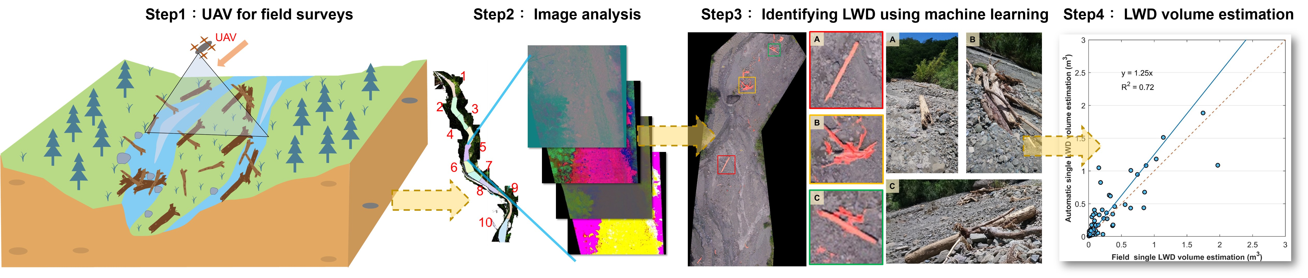
:Large woody debris (LWD) strongly influences river systems, especially in forested and mountainous catchments. In Taiwan, LWD are mainly from typhoons and extreme torrential events. To effectively manage the LWD, it is necessary to conduct regular surveys on river systems. Simple, low cost, and accurate tools are therefore necessary. The proposed methodology applies image processing and machine learning (XGBoost classifier) to quantify LWD distribution, location, and volume in river channels. XGBoost algorithm was selected due to its scalability and faster execution speeds. Nishueibei River, located in Taitung County, was used as the area of investigation. Unmanned aerial vehicles (UAVs) were used to capture the terrain and LWD. Structure from Motion (SfM) was used to build high-resolution orthophotos and digital elevation models (DEM), after which machine learning and different color spaces were used to recognize LWD. Finally, the volume of LWD in the river was estimated. The findings show that RGB color space as LWD recognition factor suffers serious collinearity problems, and it is easy to lose some LWD information; thus, it is not suitable for LWD recognition. On the contrary, the combination of different factors in different color spaces enhances the results, and most of the factors are related to the YCbCr color space. The CbCr factor in the YCbCr color space was best for identifying LWD. LWD volume was then estimated from the identified LWD using manual, field, and automatic measurements. The results indicate that the manual measurement method was the best (R2 = 0.88) to identify field LWD volume. Moreover, automatic measurement (R2 = 0.72) can also obtain LWD volume to save time and workforce.

1. Introduction
Typhoons and torrential rains destabilize slopes to cause slope failure and debris flows. Large woody debris (LWD) along with water and sediments are subsequently introduced in most river channels. In addition, wildfires are increasingly influencing the recruitment of LWD in rivers [1,2]. In several studies [3,4,5], LWD refers to downed and dead wood pieces that are 10 cm in diameter and 1 m in length. They often alter the topography of rivers [6,7], resistance to flow, flow velocity [8], and sediment transport capacity [8,9]; influence organic matter content [10]; and enhance the biodiversity of habitat and the environment [11]. Additionally, the transportation and accumulation of LWD in river channels may destroy artificial river structures such as bridges and dikes, and may block the river to produce log jams, which would in turn escalate flood disasters and cause human life and property loss [12]. Henceforth, the study of LWD transport and accumulation has attracted the scientific community [13,14,15]. In Taiwan, the primary preventive measure against such disasters is to remove LWD from rivers directly. However, several authors have shown that the LWD accumulated in rivers are beneficial to river ecology and habitat diversity [16] and that their removal should be accompanied by compelling evidence to cause a disaster [17]. Therefore, it is crucial to understand their interaction with landform, hydrology, and ecology in rivers.
Understanding the status and location of LWD may contribute towards their modeling and in the assessment of whether they would cause secondary disasters. With an increase in the development of Structure from Motion (SfM) photogrammetry technology, there has been wide adoption of this technology in the building of terrain surfaces and terrain modeling [18,19], which could be applied to LWD mapping. Rusnák et al. [20] established a high-resolution orthophoto and DEM to perform a supervised classification and identification of LWD in a river based on the Red Green Blue (RGB) image characteristics and used the DEM to estimate volume. The authors applied the volume analysis tool in the Topolyst software to calculate and quantify the wood mass volume by determining the wood/air volume ratio [21] in different types of stacked materials. Three types of LWD accumulation were proposed: trunks, log jams, and shrubs and their air ratios were 18%, 90%, and 93%, respectively. Spreitzer et al. [22] applied SfM photogrammetry to explore the differences in the geometric shape and volume of LWDs caused by different modeling modes. Windrim et al. [23] used high-resolution and color mosaic images taken and generated by Unmanned Aerial Vehicle (UAV) and machine learning to identify LWD and compute volume.
Besides the application of SfM, machine learning algorithms have been applied to predict and evaluate natural disasters such as floods [24,25,26], groundwater [27,28,29], landslides [30,31], wildfires [32], etc. Casado et al. [33] presented a UAV based framework for identifying hydro-morphological features from high resolution RGB aerial imagery using a novel classification technique based on Artificial Neural Networks (ANNs). There are, however, limited studies on the application of machine learning to identify LWD [23,33]. This could be attributable to the mobility of LWD as they can be easily influenced by their surrounding environment, leading to different identification conditions. Besides, the size of LWD accumulation in river channels is generally too small to identify through satellite images. Moreover, with the increasing availability of high-resolution images and the rapid development of machine learning, many different classifiers have been proposed, including random forests, decision trees, support vector machines (SVM), and extreme gradient boosting (XGBoost), etc.
The combination of UAVs technology and machine learning has advanced the detection of objects within any landscape. Their low cost, high mobility, and high spatial resolution (up to 10 cm and vertical errors of up to 50 cm) have been a major boost [20]. UAVs have been widely adopted in monitoring river vegetation dynamics [34] and riparian forests [35]. The increased spatial resolution means the same object in the image is composed of many pixels so that image features can be extracted from each pixel and adjacent pixels, and the image features can identify the object. Standard image features include shape, size, pattern, color, texture, shadow, location, and association [36]. Since the size of LWD is a relatively small object in the image, and their accumulation method is rather complex, the image characteristics of LWD are identified mainly by color. Color is composed of three elements: hue, value, and chroma. Hue represents the name of the color such as red, yellow, green, blue, etc. Value represents the color’s degree of lightness and darkness, while chroma represents the degree of color turbidity. The RGB color space often expresses the presentation of colors. The information of the RGB color space mixes chroma and lightness and has uneven characteristics, so it is not easily used in color recognition [37]. The hue, lightness, chroma, and intensity information of colors can be separated by converting to other color spaces. Commonly used color spaces include YCbCr, HSV, normalized color coordinates (NCC), and CIE lab color space. The YCbCr color space is a digital algorithm for video information and has become a widely used model in digital video. The Y in YCbCr is the luminance component, and Cb and Cr represent the chrominance component [38]. The HSV color space represents the points in the RGB color model in a cylindrical coordinate system where H is hue, S is saturation, and V is lightness [37]. The CIE lab color space is about the uniformity of perceived colors. In this color space, the ab calculation of luminance (L) and chromaticity is obtained by non-linear mapping of XYZ coordinates [38].
According to [37], the effect of using original color space (RGB) in natural image identification is limited, so this study used image processing technology to generate different color space information. We used UAV to capture a river channel, and SfM technology is used to construct orthophotos. The collinearity comparative analysis of the Variance Inflation Factor (VIF) is used to screen out the factor combinations suitable for LWD identification. Then, machine learning (XGBoost) is used to identify the LWD in the river. A confusion matrix is used to analyze the color space combined with a better identification effect and the proposed most suitable color space for LWD identification. In addition, the volume of a single wood is estimated from field investigations. This is then compared with the computed volume from our applied algorithm.
2. Materials and Methods
2.1. Study Area
The study area is Nishueibei River, a tributary of the Beinan River in Taitung County (Figure 1a,b). The downstream outlet is the Fugang fishing port of Taitung County, which connects Lanyu and Green Island. The Nishueibei River (Figure 1c) originates from the west coastal mountains of Taiwan, with an elevation range of 270 to 600 m. The watershed area is 2.7 km2, and the main tree species are Taiwan Phoebe, Autumn Maple Tree, Mountain Fig, etc. The geological conditions are composed of mudstone and tuff sandstone. The mainstream length is about 2.8 km; moreover, this study was limited to 2 km, as shown in Figure 1d due to complex terrain and tree canopy. Extreme storm events often confront the study area. In August 2009, Typhoon Morakot caused LWD to accumulate at the Fugang fishing port, disrupting the port’s normal operations. Typhoon Fitow, in October 2013, introduced LWD in the port such that it obstructed ships and damaged the hull. In September 2016, Typhoon Megi accumulated LWD in the embarkment and affected the entry of large fish boats and passenger ships. Typhoon Bailu in 2019 affected the navigation operations of fishing vessels and passenger ships (Figure 1e).
2.2. Field Investigations
The field mission was carried out from 26–29 August 2019, and was divided into four stages. First, UAV was used to obtain the topography of the study area. Secondly, the ground control points were arranged along the river channel, and a total station measured the coordinates and elevation of each control point. Third, the UAV was applied to capture the landform of the river channel. Finally, a tape was used to manually measure the size of LWD in the river. Field survey tools during the investigation include UAV (DJI Phantom 4), total station (model Nikon DTM332), benchmarking, and ground control points (GCPs). The UAV was equipped with a RGB camera (f/2.8 focus at infinity, shutter speed 8 to 1/8000 s, and ISO range of 100 to 1600), four controlled rotors, and an on-board navigation system with inertial sensors and GPS, and endurance of approximately 25 min. GCPs were made of paper to minimize their impacts on the environment and a total of 78 GCPs were established (0.4 m2 with a bullseye marking).
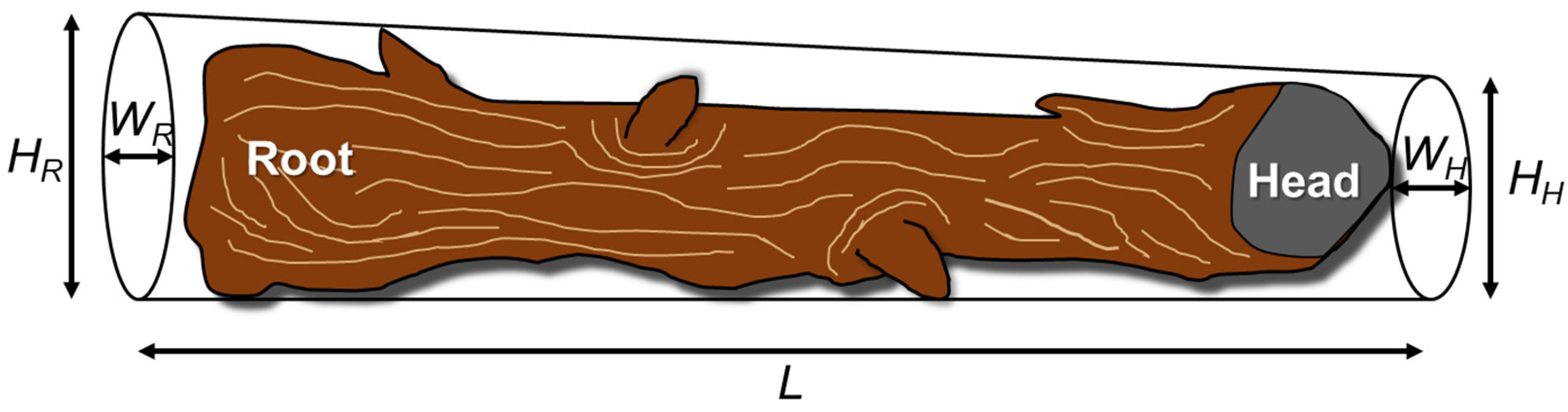
According to [20], to establish high-resolution orthophotos and numerical elevation models, different aerial photography methods such as nadir (the images with 80% forward overlap and 70% side overlap), oblique, and horizontal can increase the overall quality of the survey. To obtain detailed river information, the flight height was limited to 15 m, further constrained by the terrain, tree canopy, and UAV safety. The resolution of the numerical elevation model could reach more than 0.02 m. This was a huge limitation as flying too low led to insufficient area coverage. Moreover, due to the aforementioned factors, a compromise had to be made. The LWD accumulation in the river is usually divided into log jams and trunks. The accumulation method of log jams is complex, and the stack of wood forms many pores, which makes estimating volume problematic. As a result, in this study, emphasis was on calculating the volume of a trunk. There were 191 single LWD and 65 log jams measured. The single LWD screening criteria were about 1 m or greater in length or 10 cm in diameter. Measurements included height, width, and length (from root to head), as shown in Figure 2 below.
2.3. Image Modeling
We applied SfM technology to create high-resolution orthophoto images and digital elevation models (DEM) using Agisoft Metashape (version 1.7, Agisoft LLC). This software automatically generates 3D models based on images. It is based on the latest multi-view 3D reconstruction technology to generate high-resolution orthoimages and numerical elevation models of absolute coordinates. This is done following the standard photogrammetric workflow in the software, which includes five critical steps: Align Photos, Optimize Photo Alignment, Build Dense Cloud, Build Mesh, and Build Texture.
2.4. LWD Identification Process
The image recognition and analysis work were mainly divided into nine stages (Figure 3). In the first stage, the on-site UAV images were used to build a digital elevation model and high-resolution orthographic images. The images provided RGB color space information. The high-resolution orthophotos were manually segmented in the second stage since they contained too much information, resulting in insufficient computer memory space (The red numbers represent the different blocks after being divided). In the third stage, the segmented images were divided into a training group and a test group, and the image location information of LWD and non-LWD in the training group was manually measured. The fourth stage used MATLAB to convert the original images into different color spaces. The fifth stage used the image location information to extract LWD and non-LWD in the training group to capture different color spaces and arrange data sets. The sixth stage used MATLAB to build box plots of LWD and non-LWD for all factors and perform factor collinearity analysis to select suitable factor combinations. The seventh stage used Python to perform the XGBoost algorithm to train the training group and predict the LWD in the test group. The predicted LWD information was processed in MATLAB through Mathematical Morphology during the eighth stage. Block division combined with the smallest border (the method is detailed in Section 2.5) was used to improve the recognition results of LWD and to eliminate noise. In the final stage, the processed data was statistically analyzed and evaluated through MATLAB, and the most suitable color space to identify LWD was proposed.
2.5. Block Division of LWD Identification
Based on the statistical analysis in Section 2.4, suitable factors for identifying LWD were confirmed. The identification result formed a binary image composed of 1 and 0, where 1 referred to LWD and 0 non-LWD. Therefore, to classify each LWD, we used a similar region growing method to segment and group the LWD identification results. This method involved marking the objects of digital connection, generating a four-neighboring window, and moving it on the grid. The window movement method started from the grid in the upper left corner (Figure 4). When the window encounters a number, it sequentially checked whether a marked number in the squares 1, 2, 3, and 4. When a mark was found, it would be analyzed with that mark, and if not, it would be re-marked. After confirming the number to be marked, the window will move according to the marked numbers and update the numbers in the five squares. The grid starts again after marking the block, as shown in Figure 5.
Based on the above results, several block marks can be generated in the grid. Some noise will form several blocks in the recognition result, and covering the smallest boundary box will produce excessive borders. Therefore, the small blocks can be eliminated according to the LWD screening criteria investigated on the spot. The shortest border in the calculation box is the representative diameter, and the longest border is the representative length. The bounding box was set to delete the block marks that do not meet.
2.6. Estimating the Volume of a Single LWD
In estimating the volume of a single LWD, we used three methods, which involved field survey volume, manually circling the outline of a single LWD, and automatically identifying the block of a single LWD.
The first method (field measurement) is explained in Section 2.2. The shape of a trunk is approximately a cylinder, and its length is the length of the two ends of a trunk, and the diameter is the average of the cross-sectional area of the head and the root of the trunk. The diameter of the calculated cross-sectional area is the average of the width and height. The volume (V) of each piece was then calculated using Equation (1):
where is the length and is the diameter of the trunk head (average of HH and WH) and is the diameter of the trunk root (average of HR and WR).
The second is manual measurement, which uses the contour of a single LWD to estimate the volume. Estimating the volume is divided into five steps. In the first step, manual measurement is done along the contour of a single LWD. In the second stage, a 10 cm outer bounding box is constructed around the contour of a single LWD (Figure 6a). In the third stage, the average elevation value in the outer bounding box is calculated. In the fourth stage, the elevation data within the contour minus the average elevation of the outer bounding box is obtained. In the final stage, the elevation data within the contour is added to obtain the volume of a single LWD (Figure 6b). Although the human eye can directly confirm the position and range of a single LWD, the misjudgment of a single LWD can be reduced. The contour selected manually will form an irregular shape, which may produce different contour shapes and uncertainties. Therefore, estimating the volume would be time-consuming, and the contour shape may be difficult to repeat.
The last method applies machine learning to identify a single LWD and to estimate the volume automatically. Estimating volume is similar to the aforementioned methods. First, machine learning is used to identify a single LWD. A 10 cm outer bounding box is generated outside the minimum bounding box (Figure 6c). The elevation data in the minimum bounding box minus the average elevation of the outer bounding box is obtained. Finally, the elevation data of all the pixel values in the minimum bounding box are added to obtain the volume of a single LWD (Figure 6d). This method is reproducible, significantly reducing the uncertainty caused by manual measurement, and estimating the volume is time-saving.
2.7. Color Space Model Conversion
RGB color space information is mixed with chrominance and luminance information and non-uniform characteristics, so it is difficult to apply to color identification and analysis [34]. The use of other color space models can separate hue, luminance, and chroma and is helpful in color recognition [37]. In this study, MATLAB was used to convert to different color spaces. The color space was mathematically converted through the RGB color space of the original image to separate the color characteristics. We analyzed and compared YCbCr (“rgb2ycbcr” function), HSV (“rgb2hsv” function), Normalized Color Coordinates (NCC), and CIE lab (“rgb2lab” function). YCbCr color space is widely used. Y stands for luminance, and Cb and Cr stand for blue, the chroma of color, and red. In the HSV color space, H stands for Hue, S stands for saturation, and V stands for luminance. NCC is to normalize RGB separately, reducing the dependence of color on brightness [39]. We replaced the processed red, green, and blue (RGB) results with nR, nG, and nB [39]. The CIE lab color space was converted from CIE XYZ. In the CIE lab, l* is the illumination component (l* = 0 means black, l* = 100 means white); a and b are chroma information where a* is the position between magenta and green (a* < 0 = green, and a* > 0 = magenta). b* is the position between yellow and blue (b* < 0 = blue, b* > 0 = yellow) [38,40,41]. The conversion process was based on the intensity of light, and l stands for luminance. The hue and chroma are functions of a and b [40,41].
The formula for converting RGB color space to CIE XYZ color space and then to CIE lab is as follows:
where Xn, Yn, Zn describe a specified white achromatic reference illuminant.
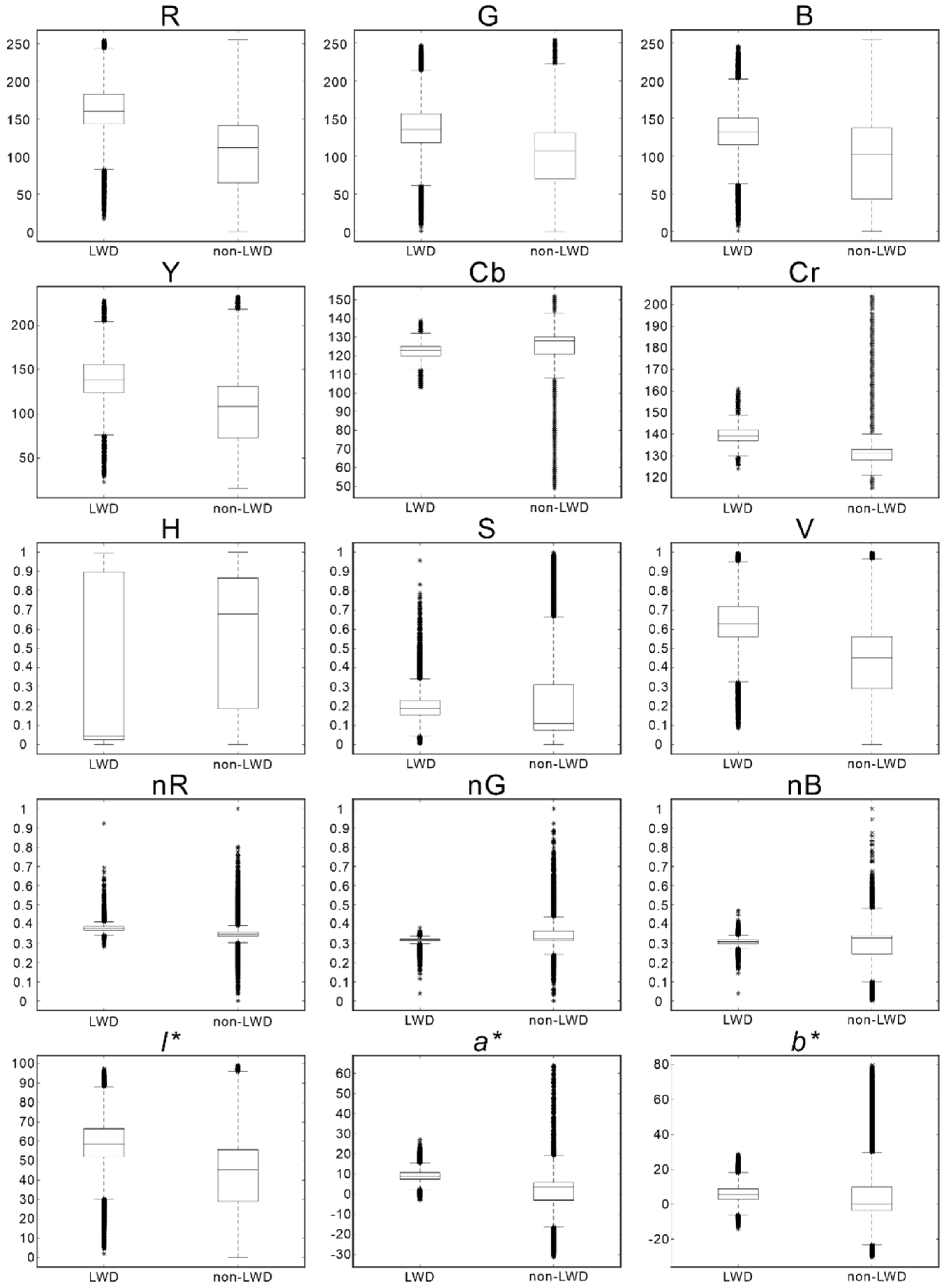
Among them, R, G, and B, respectively, represent the three components in the RGB color space. After the color space conversion, 15 factors were obtained: R, G, B, Y, Cb, Cr, H, S, V, nR, nG, nB, l*, a*, b*. LWDs were selected in different color spaces, and a color space suitable for their identification was selected.
2.8. XGBoost Model
The machine learning classifier used in this study is XGBoost. Among the basic algorithms of machine learning in recent years, the XGBoost classifier has been widely used in modern industries. The main advantage of XGBoost is its scalability and execution speed, which are far better than other machine learning algorithms [43]. Manju et al. [44] noted that models have a bias towards classes with more samples. They also tend to predict only the majority class data as features of the minority class are often treated as noise and therefore ignored. As a result, the authors proposed an ensemble classification model using XGboost to enhance the performance of classification. Compared with other models, XGBoost proved better classification accuracy when dealing with classification problems [44]. We used Python libraries to implement all XGBoost processes. XGBoost is derived from the boosting algorithm and is a robust classifier composed of multiple weak classifiers. It is a collection of multiple decision trees (CART) to form an enhanced classifier [45]. In the XGBoost algorithm, a predictive model is built by combining iteratively the best randomly generated regression trees that improve the model performance by means of a specific objective function. The following formula expresses the objective function (Obj):
Two different parts make this objective function: the leftmost part is the loss term (), which measures the differences between the predicted () and the measured () values; the rightmost part is the regularization term (), which is used to control the complexity of the model. Regularization tends to choose simple models to avoid overfitting. The k represents the number of decision trees. The objective function determines the ensemble of those regression trees that simultaneously improve the model’s prediction and minimize the model’s complexity [45].
2.9. Model Evaluation
Many studies have proposed different evaluation models based on the results of machine learning. This study focused on characterizing images into LWD and non-LWD, and the most used model evaluation method, the confusion matrix, was used. The confusion matrix is the comparison between predicted results and actual results. The comparison results are expressed as true positive (TP), true negative (TN), false positive (FP), and false negative (FN). A better prediction model is selected based on the evaluation index obtained after calculation. Evaluation indicators include precision, recall, and harmonic mean (F1). Since it is difficult to find a relatively ideal factor by referring to the results of Precision or Recall alone, F1, which is the average of the two indicators is often applied.
3. Results
3.1. Training and Test Data Selection
Due to the limitation of computational power, the built Agisoft orthophoto was cut into 20 blocks. Some of these blocks had no LWD accumulation, or the river channel were obstructed by dense tree canopy. In addition, some were damaged. All the photos in these categories (seven blocks in total) were discarded and excluded from the analysis. The 5th, 6th, 7th, and 8th blocks formed the test group, while 9 of the remaining blocks formed the training group (Figure 7). The spatial resolution of the high-resolution image created was 2 cm × 2 cm.
3.2. Filtering the Factors of the Color Space Model
Five color spaces were used to identify LWD, and the number of factors after conversion were 15. The data distribution of each factor on LWD and non-LWD are shown in Figure 8. The trends of R, G, and B factors are similar. LWD distribution is concentrated in the middle, while the range of maximum and minimum values of non-LWD almost covers the distribution of the entire data, making it difficult to distinguish between LWD and non-LWD. The YCbCr color space results show that the Y factor’s non-LWD data are widely distributed, and the data of the Cb and Cr factors of LWD and non-LWD are narrower. Therefore, the Cb and Cr factors can easily separate LWD than the Y factor. In addition, LWD is misaligned with the interquartile range (IQR) of the non-LWD Cr factor. In the HSV color space, the data distribution of the H factor of LWD and non-LWD is extensive, covering almost the entire data distribution, so it is challenging to distinguish LWD. The IQR of the S-factor LWD data is included in the IQR of the non-LWD data, again making it difficult to distinguish the LWD. In the NCC color space, the maximum and minimum values of LWD and non-LWD, and the data distribution of IQR are narrow, and the distribution positions are almost similar. Therefore, the NCC color space is less suitable for distinguishing LWD. The results of the CIE lab color space show that the data distribution of the l* factor is similar to that of the Y and V factors. The a* factor is similar to the Cr factor, and the IQR of LWD and non-LWD data are staggered, such that it is easy to distinguish LWD. The b* factor is similar to the S factor. The IQR of LWD is included in the IQR of non-LWD data, making it difficult to distinguish LWD. The data presented by the box plot is to observe the data distribution in one-dimensional, but in the subsequent identification, LWD is identified in a multi-dimensional manner. Therefore, the box plot (in Figure 8) is mainly to get a preliminary understanding of the data distribution.
Multicollinearity between factors will seriously affect the analysis results and trends. Henceforth, we used the variance inflation factor (VIF) to determine whether serious multicollinearity exist between the factors (Table 1). When the VIF < 5, there is no collinearity; 5 VIF 10, there is a moderate degree of collinearity; VIF > 10, there is severe collinearity [46]. Groups 1 to 5th are the analysis results of the five color spaces. The results show that the VIF value of the RGB color space is greater than 10, suggesting serious collinearity among R, G, and B, so the RGB color space is not suitable for analysis. In other terms, the factor information in the RGB color space mixes the features in the image, leading to serious collinearity. In groups 6th to 16th, which used a combination of different color spaces (except RGB color space), the different color spaces separated the different information of the image. At least three groups with a VIF value of < 10 were selected for predictive analysis. From the 6th and 14th groups Y, V, and l* have obvious collinearity among them. From the 9th group of data, the results of the VIF value without Y, V, and l* factors indicate that there is no obvious collinearity. This shows that Y, V, and l* are similar, and the results are consistent with the color space conversion description; they describe the luminance of the image.
After analyzing the VIF value, 11 groups were selected for LWD identification, and the samples in the 5th block were used to explore which combination is most suitable for LWD identification. Table 2 shows that in addition to the common RGB color space, recall of other combinations exceeds 80%, and F1 exceeds 70%. From the Recall, Y Cb Cr nB (84.20%) is the best among all combinations, followed by H S V a* b* (84.03%). From the Precision, Cb Cr H (69.43%) is the best among all combinations, followed by Y Cb Cr (68.22%). F1 is the average result of Recall and Precision, which can be used as a single index to compare the result easily. From the F1, the best is Cb Cr H (75.82%), followed by Y Cb Cr (74.90%). According to the results of the box-and-whisker plot above, the IQR of the H factor almost covers the entire data distribution, making it difficult to distinguish LWD from non-LWD. This illustrates that the Cb Cr factor is an important factor in LWD identification. This result is also confirmed in the Cb Cr group data in Table 2, which means LWD identification can be made directly using the Cb Cr factor.
3.3. LWD Identification
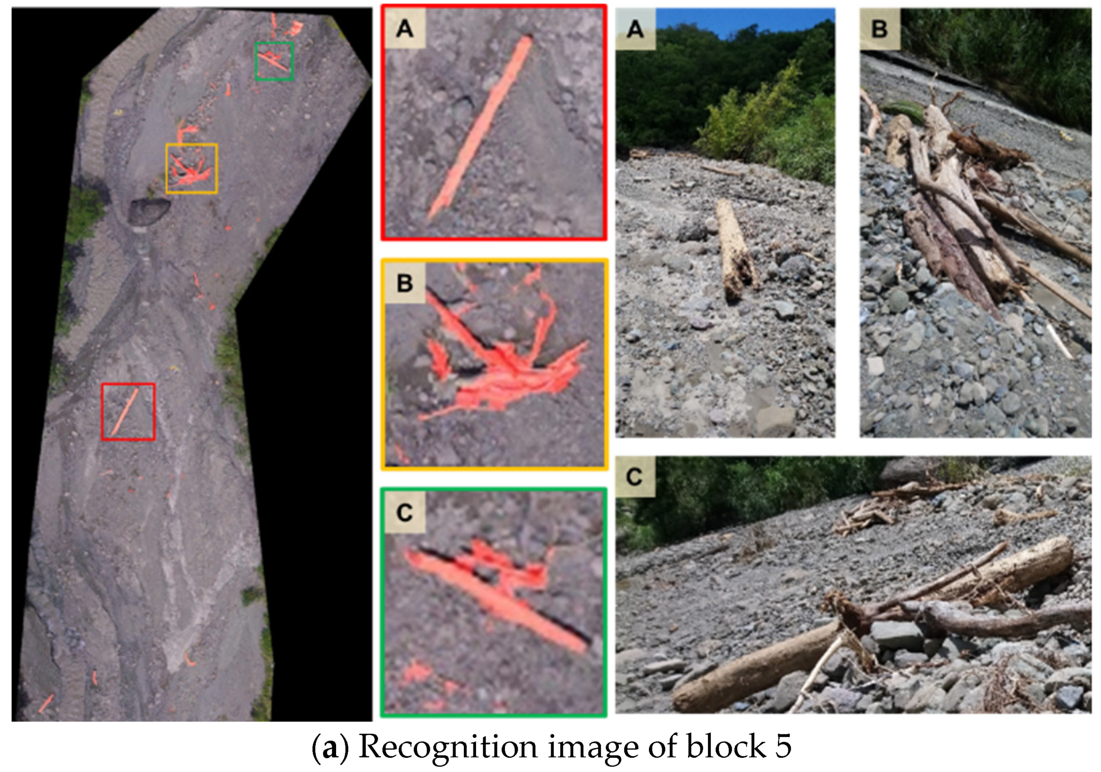
Image analysis and machine learning were used to identify LWD from orthophotos. After factor screening, Cb and Cr in the YCbCr color space were selected as the key factors to identify LWD. Identified LWD are shown in red blocks (Figure 9), and the corresponding binary classification confusion matrix for each block is shown in Table 3. The analysis results show that the recall rate of the 5th block LWD is 82.34%, and the precision is 69.28%; the recall rate of the 6th block is 69.69%, and the precision is 85.62%. The recall rate of the 7th block is 88.46%, and the precision is 88.25%; the final recall rate of the 8th block is 87.91%, and the precision is 90.97%. The reason for the lower accuracy in the 5th and 6th blocks is that there are many small groups of dead plant material in the river, which leads to the misjudgment of LWD. The 6th block contained the finest grass material and broken wood among them. The content of plant residues in the 7th block and the 8th block are obviously less, which enhanced LWD identification.
The results in Section 3.2 show a collinearity problem when using the RGB color space, which makes image recognition prone to errors. In the image recognition result (Figure 10), using the RGB color space missed more LWD information than the CbCr factor. This could have implications in the computation of LWD volume.
A similar area growth method was applied to divide the identified result block such that different LWD blocks were generated in the grid. The minimum bounding box in all the blocks were then drawn. In the field survey, the measurement condition of a single LWD was to take wood with a diameter greater than 10 cm or a length greater than 1 m (detailed in Section 2.2). Through the geometric characteristics of the minimum bounding box, it can be noted that the short side represents the diameter, and the long side represents the length. The length attribute was used to filter the identification results. The minimum bounding box with a diameter of less than 10 cm or a length of less than 50 cm (Figure 11) was deleted. The purpose of such screening was to eliminate the misjudgment of LWD and objects that were too small through the characteristics of LWD size. The result of the confusion matrix after screening shows that using the geometric characteristics of the minimum bounding box to screen can improve the identification effect of a single LWD (Table 4). In the four regions, recall decreased by 0.38% on average, precision increased by 6.76% on average, and F1 increased by 3.09% on average. Among them, the accuracy improvement in Block 6 proved to be effective in eliminating fine grass and debris at most.
3.4. The Single LWD Volume Estimation Results
This study used three methods to estimate the volume of a single LWD. The first was to evaluate the volume of a single LWD according to Equation (1) (Field). The second method was to estimate the volume of a single LWD using manual measurement (manual) and simulate the artificial identification of a single LWD. The third was to automatically identify a single LWD and use the smallest bounding box to estimate the volume (detailed in Section 2.6) (automatic). The measurement information of a single LWD in different blocks and the volume results of the different estimation methods are shown in Table 5. A total of 116 single LWD were surveyed and measured on-site in 13 blocks, of which 89 single LWD were successfully identified. The field volume results showed that the unidentified volume accounted for 2.8% of the total volume. The total volume difference between automatic and manual is 1.68 m3. Table 5 shows the range of length, head diameter, and root diameter of a single LWD in each block. The volume estimation result of the automatic measurement is almost larger than the other two methods. This is because most of the minimum frame coverage used by automatic measurement is larger than that of manual measurement, which leads to an overestimation of the field measurement in the volume estimation result.
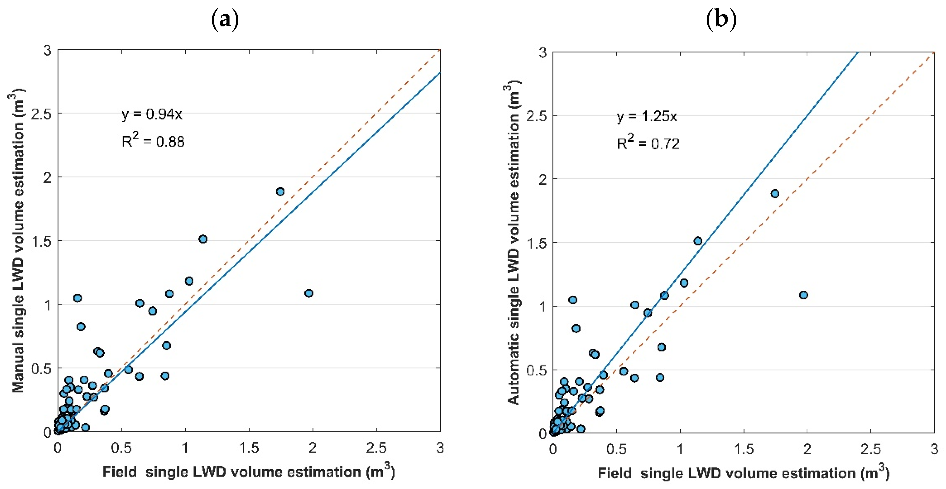
Since the second and third methods both use the elevation data to calculate the volume, the volume estimation trends are similar, indicating a system error between manual and automatic methods. Generally, the range covered by the minimum frame is larger than the range selected by manual selection. When estimating the volume of LWD, some elevation data of a single LWD connected to the ground will be added, and a small amount of gravel will be covered at the same time, which will increase the volume. The method of manual circle selection is to circle along a single LWD contour, which covers a smaller range when estimating the volume, thus making the volume smaller than the automatic measurement volume estimation. There are very few cases in which the minimum frame fails to fully cover a single LWD, making the volume smaller than that of the manual circle. From the manual and automatic driftwood volume results (Figure 12a) (R2 = 0.88), the slope is 0.94, indicating that the single LWD volume estimated by the manual method is very close to the field measurement. The results of the volume of the automatic and in-situ are shown in Figure 12b (R2 = 0.72). Volume estimates from field measurements assume a single LWD is a cylinder. Calculated using the geometric volume formula of the cylinder, the diameter of the cylinder is the average of the head and root dimensions. Therefore, it is susceptible to errors caused by bumps at both ends. The volume of wood is calculated by multiplying the cross-sectional area and length by the diameter. Therefore, the volume results measured in situ contain some air. The volume measured automatically contains some air and a small amount of surrounding gravel, so the slope between the field and the automatic will be greater than 1 (the slope is equal to 1.25). The volume estimation results show that using manual measurements is closer to the results of field measurements than automatic measurements. However, manual measurement requires a lot of manpower and time. To estimate the volume of a single LWD more quickly, the on-site measurement result can be obtained by dividing the automatic measurement result by 1.25.
4. Discussion
This study used image analysis to convert the RGB color space of orthophotos into four color models and selected suitable combinations for analysis through statistical analysis of various color space combinations. Machine learning was applied to identify the LWDs. The identification results show that the CbCrH factor combination ranked high followed by the YCbCr factor combination. The analysis result of the box plot shows that the H factor cannot effectively identify LWD. Therefore, we believe that the combination of CbCr is an essential factor in determining LWD. Past studies have shown that RGB color space information is mixed with chroma and lightness information, resulting in poor color recognition [37]. Therefore, conversion to other color spaces is needed to analyze the color information. The study also conducted the statistical analysis and LWD identification for the factors of RGB color space. The findings show that the upper and lower quartile range of the non-LWD covers almost the entire distribution of the data, such that it is challenging to distinguish LWD from non-LWD. In the VIF analysis, the RGB color space has a collinearity problem, which makes the image recognition result prone to unexpected effects. The LWD recognition result shows that using the RGB color space misses part of the LWD information than using the CbCr factor. Missing the LWD location will result in incorrect block division. Therefore, the sensitivity to finding LWD is low, which is consistent with the results of [37].
We need high-coverage images to create high-precision orthoimages and DEMs, then achieve good prediction and volume estimation. This study used different aerial photography methods in nadir, oblique, and horizontal directions to improve the coverage of the image. However, in actual field survey operations, there are many standing trees in some river sections, and the canopy can easily cover the river course, which brings difficulties to the operation and shooting of the drone. This resulted in damage to some orthophoto damaged. Subsequently, 13 blocks from the initial 20 ended up being used.
The highlight of this study was to use a simple and quick way to identify LWD in the river. We only used a color space model and machine learning (XGBoost) to complete the identification task. To note, a river channel is composed of more than LWDs; there is also the presence of gravel, fine, dry herbs, etc. In some of these components, their colors are close to LWD. For example, the color of dry weeds similar to the color of LWD provides false information. Blocks 5 and 6 contain many small groups of such material, especially the 6th block, which contains the most enormous amount of dry grass and broken wood; therefore, the recognition results of the other two blocks were poorer. In the future, it is suggested that more types of identification can be carried out for the river, and the identification effect can be improved through the characteristics of different classifications.
In terms of volume estimation of a single LWD, this study adopted three-volume estimation methods: field, manual, and automatic. The manual and field volume estimation results are similar (R2 = 0.88), which requires manual interpretation and thus consumes workforce and time. The volume estimation result of the automatic measurement is obviously larger than the field and manual results. The main reason is that the minimum frame coverage includes the elevation data of a single LWD connected to the ground. Manual and automatic volume estimates tend to be similar and subject to systematic errors. Because the automatic and field estimation methods are quite different, there are many errors in the volume estimation, and the analysis results show that the correlation of the volume estimation is only 0.72. The manual measurement method can accurately estimate the volume of a single LWD in the channel. Considering the time-saving and manpower constraints, an automatic estimation method can estimate the volume of a single LWD on-site but divided by 1.25. It is suggested that in the future, LWD types can be classified according to different types and sizes of LWD before the volume is automatically and on-site estimated, and correction values for automatic conversion of field volume estimation can be provided for different classifications. Improving the method for estimating LWD to incorporate jams LWD allows for a complete quantification of the volume of LWD in the channel.
5. Conclusions
This study used image processing and machine learning to identify LWD and to estimate the volume of a single LWD. LWD was surveyed and measured through field investigations and the use of UAVs to take images in the test area. Agisoft Metashape was used to build numerical elevation models and high-resolution orthophotos. MATLAB was used for image processing to convert the original image into different color spaces (including YCbCr, HSV, Normalized Color Coordinates (NCC), and CIE lab). DEM was used for automatic and manual single LWD volume estimation. The findings show that using the Cb and Cr factors in the YCbCr color space is an important combination for identifying LWD. When the RGB color space is used to identify LWD, there is a serious collinearity problem among various factors, and the incomplete LWD recognition effect may easily lead to the loss of some LWD data. Therefore, it is not recommended to identify LWD directly. The Cb and Cr factor can successfully identify LWD, but it is still susceptible to dry grass/vegetation in the river. Using the morphological characteristics of LWD may improve the identification effect and overcome this problem. In conclusion, manual measurement illustrates better results to estimate the volume of a single LWD. Moreover, to save time-saving and workforce constraints, we recommend using automatic measurement to obtain field volume, but it was divided by 1.25 to fit the LWD volume.
Author Contributions
Conceptualization and supervision, S.-C.C.; methodology, original draft preparation, and formal analysis, M.-C.L.; software, validation, writing—review and editing, S.S.T. All authors have read and agreed to the published version of the manuscript.
Funding
This research was funded by the Soil and Water Conservation Bureau, Taiwan, under the grant SWCB-109-024. This research was funded by the Ministry of Science and Technology, Taiwan, under the grant MOST 108-2313-B-005-019-MY3.
Data Availability Statement
This study’s datasets [GENERATED/ANALYZED] are available on request.
Acknowledgments
The authors are thankful to the graduate students of River Morphology Laboratory, Department of Soil and Water Conservation, National Chung Hsing University, for their assistance during field investigations.
Conflicts of Interest
The authors declare no conflict of interest and the funders had no role in the design of the study; in the collection, analyses, or interpretation of data; in the writing of the manuscript, or in the decision to publish the results.
References
- Vaz, P.G.; Warren, D.R.; Pinto, P.; Merten, E.C.; Robinson, C.T.; Rego, F.C. Tree type and forest management effects on the structure of stream wood following wildfires. For. Ecol. Manag. 2011, 262, 561–570. [Google Scholar] [CrossRef]
- Short, L.E.; Gabet, E.J.; Hoffman, D.F. The role of large woody debris in modulating the dispersal of a post-fire sediment pulse. Geomorphology 2015, 246, 351–358. [Google Scholar] [CrossRef]
- Wohl, E.; Scott, D.N. Wood and sediment storage and dynamics in river corridors. Earth Surf. Processes Landf. 2017, 42, 5–23. [Google Scholar] [CrossRef] [Green Version]
- Ravazzolo, D.; Mao, L.; Picco, L.; Lenzi, M.A. Tracking log displacement during floods in the Tagliamento River using RFID and GPS tracker devices. Geomorphology 2015, 228, 226–233. [Google Scholar] [CrossRef] [Green Version]
- Mao, L.; Ugalde, F.; Iroume, A.; Lacy, S.N. The Effects of Replacing Native Forest on the Quantity and Impacts of In-Channel Pieces of Large Wood in Chilean Streams. River Res. Appl. 2017, 33, 73–88. [Google Scholar] [CrossRef] [Green Version]
- Montgomery, D.R.; Collins, B.D.; Buffington, J.M.; Abbe, T.B. Geomorphic effects of wood in rivers. Ecol. Manag. Wood World Rivers 2003, 37, 21–47. [Google Scholar]
- Chen, S.-C.; Tfwala, S.S.; Wang, C.-R.; Kuo, Y.-M.; Chao, Y.-C. Incipient motion of large wood in river channels considering log density and orientation. J. Hydraul. Res. 2020, 58, 489–502. [Google Scholar] [CrossRef]
- Manners, R.B.; Doyle, M.W.; Small, M.J. Structure and hydraulics of natural woody debris jams. Water Resour. Res. 2007, 43, 1–17. [Google Scholar] [CrossRef]
- Wohl, E.; Beckman, N. Controls on the Longitudinal Distribution of Channel-Spanning Logjams in the Colorado Front Range, USA. River Res. Appl. 2014, 30, 112–131. [Google Scholar] [CrossRef]
- Diez, J.R.; Elosegi, A.; Pozo, J. Woody debris in north Iberian streams: Influence of geomorphology, vegetation, and management. Environ. Manag. 2001, 28, 687–698. [Google Scholar] [CrossRef]
- Fausch, K.D.; Northcote, T.G. Large Woody Debris and Salmonid Habitat in a Small Coastal British Columbia Stream. Can. J. Fish. Aquat. Sci. 1992, 49, 682–693. [Google Scholar] [CrossRef]
- de Paula, F.R.; Ferraz, S.F.; Gerhard, P.; Vettorazzi, C.A.; Ferreira, A. Large woody debris input and its influence on channel structure in agricultural lands of Southeast Brazil. Environ. Manag. 2011, 48, 750–763. [Google Scholar] [CrossRef]
- Máčka, Z.; Kinc, O.; Hlavňa, M.; Hortvík, D.; Krejčí, L.; Matulová, J.; Coufal, P.; Zahradníček, P. Large wood load and transport in a flood-free period within an inter-dam reach: A decade of monitoring the Dyje River, Czech Republic. Earth Surf. Processes Landf. 2020, 45, 3540–3555. [Google Scholar] [CrossRef]
- Mao, L.; Ravazzolo, D.; Bertoldi, W. The role of vegetation and large wood on the topographic characteristics of braided river systems. Geomorphology 2020, 367, 107299. [Google Scholar] [CrossRef]
- Galia, T.; Macurová, T.; Vardakas, L.; Škarpich, V.; Matušková, T.; Kalogianni, E. Drivers of variability in large wood loads along the fluvial continuum of a Mediterranean intermittent river. Earth Surf. Processes Landf. 2020, 45, 2048–2062. [Google Scholar] [CrossRef]
- Martin, D.J.; Pavlowsky, R.T.; Harden, C.P. Reach-scale characterization of large woody debris in a low-gradient, Midwestern USA river system. Geomorphology 2016, 262, 91–100. [Google Scholar] [CrossRef]
- Ortega-Terol, D.; Moreno, M.A.; Hernández-López, D.; Rodríguez-Gonzálvez, P. Survey and Classification of Large Woody Debris (LWD) in Streams Using Generated Low-Cost Geomatic Products. Remote Sens. 2014, 6, 11770–11790. [Google Scholar] [CrossRef] [Green Version]
- Morgan, J.A.; Brogan, D.J.; Nelson, P.A. Application of Structure-from-Motion photogrammetry in laboratory flumes. Geomorphology 2017, 276, 125–143. [Google Scholar] [CrossRef] [Green Version]
- Smith, M.W.; Carrivick, J.L.; Quincey, D.J. Structure from motion photogrammetry in physical geography. Prog. Phys. Geogr. Earth Environ. 2015, 40, 247–275. [Google Scholar] [CrossRef] [Green Version]
- Rusnák, M.; Sládek, J.; Kidová, A.; Lehotský, M. Template for high-resolution river landscape mapping using UAV technology. Measurement 2018, 115, 139–151. [Google Scholar] [CrossRef]
- Thevenet, A.; Citterio, A.; Piegay, H. A new methodology for the assessment of large woody debris accumulations on highly modified rivers (example of two French Piedmont rivers). Regul. Rivers: Res. Manag. 1998, 14, 467–483. [Google Scholar] [CrossRef]
- Spreitzer, G.; Tunnicliffe, J.; Friedrich, H. Using Structure from Motion photogrammetry to assess large wood (LW) accumulations in the field. Geomorphology 2019, 346, 106851. [Google Scholar] [CrossRef]
- Windrim, L.; Bryson, M.; McLean, M.; Randle, J.; Stone, C. Automated Mapping of Woody Debris over Harvested Forest Plantations Using UAVs, High-Resolution Imagery, and Machine Learning. Remote Sens. 2019, 11, 733. [Google Scholar] [CrossRef] [Green Version]
- Lee, S.; Panahi, M.; Pourghasemi, H.R.; Shahabi, H.; Alizadeh, M.; Shirzadi, A.; Khosravi, K.; Melesse, A.M.; Yekrangnia, M.; Rezaie, F.; et al. SEVUCAS: A Novel GIS-Based Machine Learning Software for Seismic Vulnerability Assessment. Appl. Sci. 2019, 9, 3495. [Google Scholar] [CrossRef] [Green Version]
- Shafizadeh-Moghadam, H.; Valavi, R.; Shahabi, H.; Chapi, K.; Shirzadi, A. Novel forecasting approaches using combination of machine learning and statistical models for flood susceptibility mapping. J. Environ. Manag. 2018, 217, 1–11. [Google Scholar] [CrossRef] [Green Version]
- Chen, W.; Li, Y.; Xue, W.; Shahabi, H.; Li, S.; Hong, H.; Wang, X.; Bian, H.; Zhang, S.; Pradhan, B.; et al. Modeling flood susceptibility using data-driven approaches of naïve Bayes tree, alternating decision tree, and random forest methods. Sci. Total Environ. 2020, 701, 134979. [Google Scholar] [CrossRef]
- Tien Bui, D.; Shirzadi, A.; Chapi, K.; Shahabi, H.; Pradhan, B.; Pham, B.T.; Singh, V.P.; Chen, W.; Khosravi, K.; Bin Ahmad, B.; et al. A Hybrid Computational Intelligence Approach to Groundwater Spring Potential Mapping. Water 2019, 11, 2013. [Google Scholar] [CrossRef] [Green Version]
- Miraki, S.; Zanganeh, S.H.; Chapi, K.; Singh, V.P.; Shirzadi, A.; Shahabi, H.; Pham, B.T. Mapping Groundwater Potential Using a Novel Hybrid Intelligence Approach. Water Resour. Manag. 2019, 33, 281–302. [Google Scholar] [CrossRef]
- Chen, W.; Pradhan, B.; Li, S.; Shahabi, H.; Rizeei, H.M.; Hou, E.; Wang, S. Novel Hybrid Integration Approach of Bagging-Based Fisher’s Linear Discriminant Function for Groundwater Potential Analysis. Nat. Resour. Res. 2019, 28, 1239–1258. [Google Scholar] [CrossRef] [Green Version]
- Tien Bui, D.; Shahabi, H.; Shirzadi, A.; Chapi, K.; Hoang, N.-D.; Pham, B.T.; Bui, Q.-T.; Tran, C.-T.; Panahi, M.; Bin Ahmad, B.; et al. A Novel Integrated Approach of Relevance Vector Machine Optimized by Imperialist Competitive Algorithm for Spatial Modeling of Shallow Landslides. Remote Sens. 2018, 10, 1538. [Google Scholar] [CrossRef] [Green Version]
- Shafizadeh-Moghadam, H.; Minaei, M.; Shahabi, H.; Hagenauer, J. Big data in Geohazard; pattern mining and large scale analysis of landslides in Iran. Earth Sci. Inform. 2019, 12, 1–17. [Google Scholar] [CrossRef]
- Jaafari, A.; Zenner, E.K.; Panahi, M.; Shahabi, H. Hybrid artificial intelligence models based on a neuro-fuzzy system and metaheuristic optimization algorithms for spatial prediction of wildfire probability. Agric. For. Meteorol. 2019, 266–267, 198–207. [Google Scholar] [CrossRef]
- Casado, M.R.; Gonzalez, R.B.; Kriechbaumer, T.; Veal, A. Automated Identification of River Hydromorphological Features Using UAV High Resolution Aerial Imagery. Sensors 2015, 15, 27969–27989. [Google Scholar] [CrossRef] [PubMed] [Green Version]
- Laslier, M.; Hubert-Moy, L.; Corpetti, T.; Dufour, S. Monitoring the colonization of alluvial deposits using multitemporal UAV RGB-imagery. Appl. Veg. Sci. 2019, 22, 561–572. [Google Scholar] [CrossRef]
- Dunford, R.; Michel, K.; Gagnage, M.; Piégay, H.; Trémelo, M.L. Potential and constraints of Unmanned Aerial Vehicle technology for the characterization of Mediterranean riparian forest. Int. J. Remote Sens. 2009, 30, 4915–4935. [Google Scholar] [CrossRef]
- Lillesand, T.; Kiefer, R.W.; Chipman, J. Remote Sensing and Image Interpretation, 7th ed.; Wiley: Hoboken, NJ, USA, 2015. [Google Scholar]
- Shaik, K.B.; Ganesan, P.; Kalist, V.; Sathish, B.S.; Jenitha, J.M.M. Comparative Study of Skin Color Detection and Segmentation in HSV and YCbCr Color Space. Procedia Comput. Sci. 2015, 57, 41–48. [Google Scholar] [CrossRef] [Green Version]
- Amanpreet, K.; Kranth, B.V. Comparison between YCbCr Color Space and CIELab Color Space for Skin Color Segmentation. Int. J. Appl. Inf. Syst. 2012, 3, 30–33. [Google Scholar]
- Soriano, M.; Martinkauppi, B.; Huovinen, S.; Laaksonen, M. Skin detection in video under changing illumination conditions. In Proceedings of the 15th International Conference on Pattern Recognition. ICPR-2000, Barcelona, Spain, 3–7 September 2000; Volume 831, pp. 839–842. [Google Scholar]
- Schloss, K.B.; Lessard, L.; Racey, C.; Hurlbert, A.C. Modeling color preference using color space metrics. Vis. Res. 2018, 151, 99–116. [Google Scholar] [CrossRef]
- Schwarz, M.W.; Cowan, W.B.; Beatty, J.C. An experimental comparison of RGB, YIQ, LAB, HSV, and opponent color models. ACM Trans. Graph. 1987, 6, 123–158. [Google Scholar] [CrossRef]
- Ford, A.; Roberts, A. Color Space Conversions; Westminster University: London, UK, 1996. [Google Scholar]
- Ruiz-Abellón, M.D.; Gabaldón, A.; Guillamón, A. Load Forecasting for a Campus University Using Ensemble Methods Based on Regression Trees. Energies 2018, 11, 2038. [Google Scholar] [CrossRef] [Green Version]
- Manju, N.; Harish, B.; Prajwal, V. Ensemble Feature Selection and Classification of Internet Traffic using XGBoost Classifier. Int. J. Comput. Netw. Inf. Secur. 2019, 11, 37–44. [Google Scholar] [CrossRef]
- Chen, T.; Guestrin, C. XGBoost: A Scalable Tree Boosting System. In Proceedings of the 22nd SIGKDD Conference on Knowledge Discovery and Data Mining, San Francisco, CA, USA, 13–17 August 2016. [Google Scholar]
- Forthofer, R.N.; Lee, E.S.; Hernandez, M. 13-Linear Regression. In Biostatistics, 2nd ed.; Forthofer, R.N., Lee, E.S., Hernandez, M., Eds.; Academic Press: San Diego, CA, USA, 2007; pp. 349–386. [Google Scholar]
Figure 1.
(a) Study area location in Taitung County, Taiwan; (b) Nishueibei River watershed in Beinan River watershed; (c) Nishueibei River watershed; (d) LWD accumulation in the research test area; (e) 26 August 2019 LWD accumulation in Fugang fishing ports.
Figure 1.
(a) Study area location in Taitung County, Taiwan; (b) Nishueibei River watershed in Beinan River watershed; (c) Nishueibei River watershed; (d) LWD accumulation in the research test area; (e) 26 August 2019 LWD accumulation in Fugang fishing ports.

Figure 2.
Illustration of single LWD measurements taken, including height (H), width (W), and length (L).
Figure 2.
Illustration of single LWD measurements taken, including height (H), width (W), and length (L).

Figure 3.
Workflow for the analysis.

Figure 4.
The four-neighbor window and the window movement method.

Figure 5.
The result of segmenting the binary graph of the original LWD and non-LWD.

Figure 6.
(a) A 10 cm outer bounding box of manual measurement, (b) inner outline of the second method, (c) a 10 cm outer bounding box of the third method, and (d) inner bounding box of the third method.
Figure 6.
(a) A 10 cm outer bounding box of manual measurement, (b) inner outline of the second method, (c) a 10 cm outer bounding box of the third method, and (d) inner bounding box of the third method.

Figure 7.
Division of the Nishueibei River test blocks.

Figure 8.
The data distribution of each factor to LWD and non-LWD.

Figure 9.
LWD identification in (a) block 5 (b) block 6, and (c) block 7. (Identified LWD are shown in red.)
Figure 9.
LWD identification in (a) block 5 (b) block 6, and (c) block 7. (Identified LWD are shown in red.)


Figure 10.
Comparison of CbCr and RGB color space in blocks 5 and blocks 6.

Figure 11.
Bounding box screening in block 5. The number represents the object number filtered by the bounding box (a) before screening, (b) after screening.
Figure 11.
Bounding box screening in block 5. The number represents the object number filtered by the bounding box (a) before screening, (b) after screening.

Figure 12.
(a) Field and manual measurements of single LWD volume estimation. (b) Field and automatic measurements of single LWD volume estimation.
Figure 12.
(a) Field and manual measurements of single LWD volume estimation. (b) Field and automatic measurements of single LWD volume estimation.


Table 1.
Calculated VIF values.
| Group | R | G | B | Y | Cb | Cr | H | S | V | nR | nG | nB | l* | a* | b* |
|---|---|---|---|---|---|---|---|---|---|---|---|---|---|---|---|
| 1 | 56.8 | 34.9 | 11.0 | ||||||||||||
| 2 | 1.5 | 1.0 | 1.6 | ||||||||||||
| 3 | 1.5 | 1.2 | 1.3 | ||||||||||||
| 4 | 7.7 | 5.4 | 2.0 | ||||||||||||
| 5 | 1.4 | 5.1 | 4.4 | ||||||||||||
| 6 | 303.1 | 4.9 | 2.2 | 2.3 | 5.9 | 301.1 | |||||||||
| 7 | 464.1 | 7.7 | 5.9 | 2.4 | 16.2 | 446.0 | 28.8 | 28.7 | 11.2 | ||||||
| 8 | 1060.6 | 310.3 | 106.7 | 2.8 | 22.5 | 563.5 | 55.6 | 52.6 | 18.0 | 1142.7 | 441.9 | 809.9 | |||
| 9 | 2.0 | 5.8 | 2.4 | 9.7 | 10.9 | 4.6 | |||||||||
| 10 | 2.7 | 17.7 | 496.9 | 46.5 | 38.0 | 13.3 | 509.7 | 35.5 | 26.2 | ||||||
| 11 | 31.3 | 25.1 | 10.2 | 2.2 | 18.5 | 17.0 | |||||||||
| 12 | 2.6 | 6.9 | 288.9 | 288.3 | 8.2 | 8.6 | |||||||||
| 13 | 2.4 | 5.6 | 4.8 | 26.0 | 20.4 | 8.6 | |||||||||
| 14 | 794.7 | 191.7 | 68.8 | 763.8 | 222.1 | 406.1 | |||||||||
| 15 | 2.2 | 4.1 | 1.7 | 2.2 | 3.4 | ||||||||||
| 16 | 2.2 | 3.5 | 2.1 | 5.7 | 7.7 |
Table 2.
Prediction results of the different color spaces and different combinations.
| Factor Combinations | TP | FN | FP | TN | Recall (%) | Precision (%) | F1 (%) |
|---|---|---|---|---|---|---|---|
| Y Cb Cr | 21,333 | 4817 | 9938 | 3,998,822 | 81.58 | 68.22 | 74.90 |
| H S V | 21,655 | 4495 | 12,122 | 3,996,638 | 82.81 | 64.11 | 73.46 |
| nR nG nB | 17,110 | 9040 | 8173 | 4,000,587 | 65.43 | 67.67 | 66.55 |
| l* a* b* | 21,898 | 4252 | 11,967 | 3,996,793 | 83.74 | 64.66 | 74.20 |
| Cb Cr H S | 21,624 | 4526 | 11,719 | 3,997,041 | 82.69 | 64.85 | 73.77 |
| Cb Cr H | 21,497 | 4653 | 9463 | 3,999,297 | 82.21 | 69.43 | 75.82 |
| H S V nR nB | 21,290 | 4860 | 10,976 | 3,997,784 | 81.41 | 65.98 | 73.70 |
| H S a* b* | 21,193 | 4957 | 9948 | 3,998,812 | 81.04 | 68.05 | 74.55 |
| Y Cb Cr nB | 22,017 | 4133 | 12,211 | 3,996,549 | 84.20 | 64.32 | 74.26 |
| Y Cb Cr H S | 21,970 | 4180 | 12,679 | 3,996,081 | 84.02 | 63.41 | 73.71 |
| H S V a* b* | 21,974 | 4176 | 12,287 | 3,996,473 | 84.03 | 64.14 | 74.08 |
| Cb Cr | 21,531 | 4619 | 9547 | 3,999,213 | 82.34 | 69.28 | 75.81 |
Table 3.
LWD identification results (CbCr).
| TP | FN | FP | TN | Recall (%) | Precision (%) | F1 (%) | |
|---|---|---|---|---|---|---|---|
| Block 5 | 21,531 | 4619 | 9547 | 3,999,213 | 82.34 | 69.28 | 75.81 |
| Block 6 | 13,549 | 5892 | 5216 | 2,756,964 | 69.69 | 72.20 | 70.95 |
| Block 7 | 57,569 | 7511 | 7662 | 3,025,384 | 88.46 | 88.25 | 88.36 |
| Block 8 | 14,021 | 1929 | 1391 | 3,387,310 | 87.91 | 90.97 | 89.44 |
Table 4.
LWD identification result (CbCr) combined with minimum bounding box screening.
| TP | FN | FP | TN | Recall (%) | Precision (%) | F1 (%) | |
|---|---|---|---|---|---|---|---|
| Block 5 | 21,455 | 4695 | 7233 | 4,001,527 | 82.05 | 74.79 | 78.42 |
| Block 6 | 13,381 | 6060 | 3266 | 2,758,914 | 68.83 | 80.38 | 74.60 |
| Block 7 | 57,385 | 7695 | 3474 | 3,029,572 | 88.18 | 94.29 | 91.23 |
| Block 8 | 14,006 | 1944 | 362 | 3,388,339 | 87.81 | 97.48 | 92.65 |
Table 5.
Measurement information of a single LWD surveyed in the field and the volume results of the different estimation methods.
Table 5.
Measurement information of a single LWD surveyed in the field and the volume results of the different estimation methods.
| Block | Amount | Loss | Length L (m) | Head DH (m) | Root DR (m) | Volume Estimation V (m3) | ||
|---|---|---|---|---|---|---|---|---|
| Field | Manual | Automatic | ||||||
| 1 | 9 | 3 | 2.01~4.44 | 0.06~0.35 | 0.08~0.35 | 0.56 | 1.21 | 2.22 |
| 2 | 21 | 2 | 0.80~4.69 | 0.09~0.40 | 0.05~0.60 | 1.78 | 1.50 | 2.93 |
| 3 * | 5 | 4 | 1.72 | 0.37 | 0.37 | 0.18 | 0.68 | 0.84 |
| 4 | 11 | 3 | 0.86~4.67 | 0.02~0.47 | 0.05~0.55 | 0.75 | 1.14 | 1.33 |
| 5 | 12 | 4 | 0.72~5.70 | 0.08~0.39 | 0.09~0.55 | 1.47 | 1.09 | 1.16 |
| 6 | 8 | 2 | 1.50~8.53 | 0.06~0.48 | 0.13~0.46 | 0.68 | 1.29 | 2.42 |
| 7 | 8 | 2 | 1.20~9.21 | 0.06~1.13 | 0.03~1.00 | 5.83 | 4.37 | 5.37 |
| 8 | 4 | 1 | 3.92~6.54 | 0.04~0.29 | 0.1~0.90 | 1.72 | 1.26 | 2.99 |
| 9 | 3 | 0 | 2.40~10.63 | 0.12~0.40 | 0.1~0.64 | 2.12 | 1.12 | 1.51 |
| 10 | 11 | 1 | 1.23~5.32 | 0.08~0.63 | 0.1~0.31 | 1.15 | 1.29 | 2.08 |
| 11 * | 4 | 3 | 10.2 | 0.46 | 0.27 | 1.14 | 1.25 | 1.96 |
| 12 | 9 | 2 | 1.23~4.33 | 0.08~0.40 | 0.06~0.44 | 0.67 | 0.92 | 1.11 |
| 13 | 12 | 0 | 1.93~13.57 | 0.13~0.65 | 0.12~0.60 | 4.60 | 4.83 | 6.52 |
| 13 | 116 | 27 | Does not include unrecognized success | 22.65 | 21.97 | 32.45 | ||
| Not recognized successfully | 0.82 | 1.68 | 0 | |||||
* Means that only one single LWD has been successfully identified in this area.
Publisher’s Note: MDPI stays neutral with regard to jurisdictional claims in published maps and institutional affiliations. |
© 2022 by the authors. Licensee MDPI, Basel, Switzerland. This article is an open access article distributed under the terms and conditions of the Creative Commons Attribution (CC BY) license (https://creativecommons.org/licenses/by/4.0/).
Share and Cite
MDPI and ACS Style
Liang, M.-C.; Tfwala, S.S.; Chen, S.-C. The Evaluation of Color Spaces for Large Woody Debris Detection in Rivers Using XGBoost Algorithm. Remote Sens. 2022, 14, 998. https://0-doi-org.brum.beds.ac.uk/10.3390/rs14040998
AMA Style
Liang M-C, Tfwala SS, Chen S-C. The Evaluation of Color Spaces for Large Woody Debris Detection in Rivers Using XGBoost Algorithm. Remote Sensing. 2022; 14(4):998. https://0-doi-org.brum.beds.ac.uk/10.3390/rs14040998
Chicago/Turabian StyleLiang, Min-Chih, Samkele S. Tfwala, and Su-Chin Chen. 2022. "The Evaluation of Color Spaces for Large Woody Debris Detection in Rivers Using XGBoost Algorithm" Remote Sensing 14, no. 4: 998. https://0-doi-org.brum.beds.ac.uk/10.3390/rs14040998
Note that from the first issue of 2016, this journal uses article numbers instead of page numbers. See further details here.