
Spaceborne GNSS Reflectometry
by
 ,
,
Kegen Yu
1,2, 
Shuai Han
1,2, 
Jinwei Bu
1,2,* ,
,
Yuhang An
1,2,
Zhewen Zhou
1,2,
Changyang Wang
1,2, 
Sajad Tabibi
3 and
Joon Wayn Cheong
4 1
MNR Key Laboratory of Land Environment and Disaster Monitoring, China University of Mining and Technology, Xuzhou 221116, China
2
School of Environment Science and Spatial Informatics, China University of Mining and Technology, Xuzhou 221116, China
3
Department of Engineering, Faculty of Science, Technology and Medicine, University of Luxembourg, 4364 Luxembourg, Luxembourg
4
The Australian Centre for Space Engineering Research Engineering, University of New South Wales, Sydney, NSW 2052, Australia
*
Author to whom correspondence should be addressed.
Remote Sens. 2022, 14(7), 1605; https://0-doi-org.brum.beds.ac.uk/10.3390/rs14071605
Submission received: 14 February 2022
/
Revised: 17 March 2022
/
Accepted: 25 March 2022
/
Published: 27 March 2022
(This article belongs to the Special Issue Recent Advances in GNSS Reflectometry)
Abstract
:This article presents a review on spaceborne Global Navigation Satellite System Reflectometry (GNSS-R), which is an important part of GNSS-R technology and has attracted great attention from academia, industry and government agencies in recent years. Compared with ground-based and airborne GNSS-R approaches, spaceborne GNSS-R has a number of advantages, including wide coverage and the ability to sense medium- and large-scale phenomena such as ocean eddies, hurricanes and tsunamis. Since 2014, about seven satellite missions have been successfully conducted and a large number of spaceborne data were recorded. Accordingly, the data have been widely used to carry out a variety of studies for a range of useful applications, and significant research outcomes have been generated. This article provides an overview of these studies with a focus on the basic methods and techniques in the retrieval of a number of geophysical parameters and the detection of several objects. The challenges and future prospects of spaceborne GNSS-R are also addressed.
1. Introduction
Global Navigation Satellite System Reflectometry (GNSS-R) is an emerging remote sensing technology. GNSS-R exploits the L-band radio signals transmitted from GNSS satellites, so that the technology is cost-effective and the device can be more compact compared with an active system equipped with both a transmitter and a receiver. GNSS-R derives the geophysical parameters of surface media and/or performs object detection by processing and analyzing the reflected signals. Observations such as signal-to-noise ratio (SNR), carrier phase and pseudorange provided by typical GNSS receivers can be used as GNSS-R data to measure geophysical parameters. For instance, thousands of continuously operating reference stations (CORS) have been established in the world for many different purposes, including relative positioning and crustal motion monitoring. CORS data have also been used for sensing the geophysical parameters of the environment around each of the stations [1]. GNSS-R observations can also be made using dedicated GNSS-R receivers. The main difference between a GNSS-R receiver and a typical GNSS receiver is that the former contains hardware and software to generate a delay–Doppler map which contains the key observation data for airborne and spaceborne GNSS-R technology. Thus, a GNSS-R receiver may be considered as an extension to a typical GNSS receiver.
In the case of ground-based signal reception, a single antenna such as a geodetic one is usually fixed on a tripod or a high post to capture both direct and reflected GNSS signals. The antenna can be placed as zenith-looking, which is typically used in CORS. The extensive data recorded by CORS are a useful resource which can be directly used to sense several geophysical parameters such as snow depth and soil moisture. Note that CORS is not designed for GNSS-R applications, and it is, in fact, that the reflected signals are greatly suppressed to enable high-quality positioning, navigation and timing services. In the non-CORS cases, the antenna may be fixed to face horizontally so that both the direct and reflected signals have similar antenna gains, to increase the reflected signal power compared with a CORS antenna setup [2]. Making use of the composite direct and reflected signals to infer properties and estimate parameters of reflection surface is also referred to as interferometric GNSS-R or interference pattern technique (IPT) [3]. When the receiver and antenna(s) are carried by an aircraft or a low Earth orbit (LEO) satellite, the reflected signals are captured by the nadir-looking antennas located on the bottom of the carrier so that the direct signals do not interfere with the reflected signals. Such a version of GNSS-R is sometimes called conventional GNSS-R. Typically, regardless of antenna placement or processing techniques, the direct signal is generally utilized to serve as a reference in terms of signal power or carrier phase.
1.1. Early Pioneering Works in GNSS-R
The concept of GNSS-R was probably first proposed by Hall and Cordey [4], about 10 years after the first global positioning system (GPS) satellite was launched in 1978, and about 5 years before GPS was operational with global coverage in 1993. When studying multistatic scatterometry, they considered performing multistatic measurements of GPS signals with a rotational antenna to measure ocean-surface wind velocity. Martin-Neira [5] proposed the use of GNSS-R for sea surface altimetry and considered the development of a passive reflectometry and interferometry system (PARIS) onboard a LEO satellite. Auber et al. [6] reported the capture of GPS signals reflected over the ocean during an airborne experiment, which was designed for the mitigation of multipath from both land and ocean to enhance a GPS-based vehicle-tracking system, but not for GNSS-R technology. Katzberg and Garrison [7] proposed the measurement of ionospheric delay using GNSS reflected signals from the ocean surface captured by LEO satellites, thus improving the accuracy of the measurements. In 1998, Garrison et al. [8] conducted several flight experiments to explore the possibility of using sea surface GPS signals to measure sea surface roughness. Kavak et al. [9] conducted ground-based GNSS-R experiments to estimate the soil surface dielectric constant and compare the relationship between the measured and modeled signal power and the satellite elevation angle. Komjathy et al. [10] used GPS signals reflected from the seawater surface to estimate the sea-surface wind speed. Then, in the next few years, Anderson [11] used GPS signals to measure water levels and ocean tides; Masters et al. [12] and Zavorotny and Voronovich [13] utilized the power variation of reflected GPS signal power to monitor soil moisture changes. Komjathy et al. [14] suggested the use of GPS signals reflected from the ocean or land surface for several applications, including wave height and salinity studies, wetland detection, and ionospheric TEC monitoring over the ocean. Zavorotny and Voronovich [15] proposed a mathematical model which describes scattered GNSS signal power as a function of geometrical, environmental, and system parameters. The model can be used to generate the delay–Doppler map (DDM), which has since been widely studied. In this model, the scattered GNSS signal power can be represented as a function of the time delay and the Doppler shift , which is given by:
where is the power of reflected GNSS signals received by the GNSS-R receiver; is the coherent integration time; stands for the GNSS signal wavelength; denotes the satellite transmitting power; and represent the antenna gain of the satellite and receiver, respectively; and represent the distance between the specular point of the reflection to the satellite and the receiver, respectively; is the PRN code auto-correlation function; is the sin function used to describe the power reduction due to the doppler frequency shift; and stands for the scattering coefficient per unit area of surface A, namely the bistatic radar cross section described by
Here, is the vector from the specular point to the scattered point; stands for the Fresnel reflection coefficient; is the scattering unit vector; and and stand for the vertical component and the horizontal component of the scattering unit vector, respectively. In October 2000, there was a NOAA Hurricane Hunter research aircraft flight experiment off the coast of South Carolina, which carried a GPS receiver and collected GPS signals from the sea surface inside Hurricane Michael during the flight [16]. Treuhaft et al. [17] conducted a high-precision coast-based experiment in which a GPS receiver was fixed to an observation point 480 m above the lake surface, and the measurements resulted in 2-cm precision when using a data average interval of 1 s. These are just some of the early pioneer works related to ground-based and airborne GNSS-R technology. More information about this innovative remote sensing technology can also be seen in several books and review articles [18,19,20,21,22,23].
1.2. GNSS-R-Related Satellite Missions
Similar to other major remote sensing technologies, there have been about 10 satellite missions with a payload for GNSS-R applications or with a main focus on specific GNSS-R application. The UK-DMC (Disaster Monitoring Constellation) satellite is the first GNSS-R-related satellite to be built by Surrey Satellite Technology Ltd. (SSTL). The UK-DMC satellite was launched on the 27 September 2003; it carried four major payloads, and one of them was designed to conduct an experiment to demonstrate the potential application of GNSS-R. Although the data collected by the UK-DMC satellite has not been widely used for remote sensing studies, probably because the amount of data is limited, the satellite indeed sensed ocean roughness [24]. On the 8 July 2014, the UK launched the TechDemoSat-1 (TDS-1) satellite, which carried the SGR-RESI (Space GNSS Receiver-Remote Sensing Instrument), also developed by SSTL. The TDS-1 satellite was retired from service in December 2018. Over the period of four years, TDS-1 has recorded a large number of data, which have been widely used for studies in science and technology [21,25,26]. Following TDS-1, on the 15 December 2016, NASA launched eight micro-satellites to monitor tropical cyclones with an initial main objective of enhancing the accuracy of the measurement and prediction of hurricane intensity [27,28]. The constellation is termed cyclone GNSS (CYGNSS) and the project has been led by the University of Michigan. CYGNSS has also produced a large number of data, which have been used to retrieve various ocean and land parameters, in addition to the original targeted one or two parameters. In the following years up to July 2021, a series of satellites have been launched to investigate the science problems and applications of GNSS-R technology. On the 14 July 2017, microsatellite WNISAT-1R was launched, which was developed by Weathernews Inc. in Japan [29]. A WNISAT-IR payload is a GNSS-R receiver that has received GNSS signals and generated delay–Doppler maps. BuFeng-1 A/B twin satellites were launched from the Yellow Sea on 5 June 2019, which was developed by the China Aerospace Science and Technology Corporation (CASTC). The primary focus of the satellite mission is to test the ability of GNSS-R to monitor sea-surface wind fields, particularly Typhoons [30,31]. On the 5 July 2019, the DOT-1 satellite was launched, and was the third satellite to be designed by SSTL and used for GNSS-R studies. The payload carried on the DoT-1 satellite is designed to test advanced electronics, such as in antenna technology, that could be used in future spaceborne technology [32]. Spire Global Inc. GNSS RO CubeSats has been providing altimetric observations from surfaces that reflect coherently at L-band since 2019. On the 3 July 2021, the first commercial satellite (Jilin-01B) with a GNSS-R payload was launched. The satellite was developed by Tianjin University in China to perform the task of sensing a range of ocean parameters. On the 5 July 2021, the FY-3E Satellite, developed by CASTC, was launched. It carries 11 payloads, including the one for integrated GNSS-RO (GNSS radio occultation) and GNSS-R for the first time, sensing parameters in the ionosphere, atmosphere and ocean [33].
1.3. Structure of the Article
The basic GNSS-R concepts, the early pioneering works and the GNSS-R related satellite missions are briefly described above. The main focus of the article is on a specific aspect of GNSS-R technology, namely spaceborne GNSS-R; this is currently a hot research topic, particularly due to the successful launch of more than 15 satellites with onboard GNSS-R sensors in the past eight years, as mentioned above. The remainder of the article is organized as follows.
Section 2 presents an overview of the use of spaceborne GNSS-R data to retrieve sea-surface wind speed, which is the wind speed at places about 10–20 m above the sea surface. Since sea-surface wind and sea waves usually co-exist, Section 2 also introduces the retrieval methods of sea-wave height (i.e., significant wave height) with spaceborne GNSS-R data. Typically, low-to-medium wind speed can be measured more accurately than high wind speed. It is more complicated to measure the intensity of very strong winds such as those of a typhoon and hurricane, partly due to the rather noisy DDM data necessitating more advanced data processing and parameter calibration.
Section 3 focuses on rainfall detection and rainfall intensity retrieval with spaceborne GNSS-R technology. There is only a limited number of papers related to this topic. These are early attempts to handle this rather difficult problem. One reason is that sea-surface wind usually dominates the sea-surface roughness so that the signature of rainfall is hard to extract, especially in the presence of strong wind. Another reason is that when rainfall is strong, the sea surface roughness may be insensitive to the variation in rainfall intensity. Thus, the problem may only be resolvable in cases where the wind speed is not very high and the rainfall intensity is not very strong.
Section 4 studies the methods and techniques used in GNSS-R spaceborne sea-surface altimetry, which is, in fact, one of the first GNSS-R applications considered. The main challenge of current altimetry with spaceborne GNSS-R data is that nearly all the satellite missions focused on the use of a delay–Doppler map (DDM) to derive variables, observables, or decision statistics to retrieve geophysical parameters. On the other hand, conventional altimetry mainly relies on the accurate measurement of time of arrival (TOA) and distance, and GNSS-R altimetry mainly uses the measurement of time difference of arrival (TDOA). Thus, advanced data processing techniques are required to improve TDOA measurement accuracy. Additionally, in this section, methods for land topography retrieval are briefly studied, and it seems that more investigations should be conducted.
Section 5 presents a review of the methods for retrieving soil moisture, which has also been an intensively investigated issue recently. It is useful to mention that microwave sensing of soil moisture has been widely investigated in recent decades, but there is still space to improve. Soil components, surface roughness and vegetation canopy make retrieving soil moisture a difficult problem. In particular, similar to ground-based and airborne sensing methods, soil moisture retrieval is greatly affected by vegetation canopy. Thus, knowledge of the vegetation canopy is required for soil moisture retrieval, and it may be obtained in two different ways. One is that the vegetation information is retrieved first, and the other is that vegetation canopy and soil moisture are retrieved jointly. The second part of the section briefly describes the methods of vegetation parameter estimation in the literature.
Section 6 provides an overview of sea ice detection based on spaceborne GNSS-R data. Since sea ice mostly exists in the Arctic and Antarctic regions, it is usually only feasible to perform sea ice detection by using satellite data, instead of conducting ground-based or airborne campaigns. Since a few major satellite missions such as CYGNSS and Bufeng-1 mainly focus on the monitoring of sea-surface wind speed, the trajectories of the satellites do not cover the two polar regions. As a result, their data cannot be used for sea ice detection. Some surface areas near the polar regions are completely covered with sea ice, while areas far from the polar regions are completely free of ice. Intuitively, there are areas (like the circular band) where the sea surface consists of both sea ice and seawater. It is useful to identify such areas where there is a mixture of sea ice and seawater and measure their sea ice concentration, the latter of which is briefly discussed in this section. Furthermore, since sea ice thickness and sea ice type (one-year or multiple-year) are important parameters of sea ice, the thickness estimation and type identification are also studied.
Section 7 presents an overview of flood and tsunami detection. In particular, spaceborne GNSS-R data were employed to detect the floods that occurred recently in China. It is useful to identify the size of the flooding area and monitor the intensity and speed of the flooding, so that proper measures can quickly be taken to minimize the damage and cost induced by the flooding. Similar to sea ice detection, spaceborne GNSS-R technology is better suited to Tsunami detection than ground-based and airborne GNSS-R technologies due to the very long wavelength (several hundred kilometers) and high propagation speed of tsunamis. Since significant tsunamis occur rarely, there are a very limited number of spaceborne GNSS-R data that contain tsunami information. Thus, only simulated tsunami data are used in the studies of tsunami detection, although real tsunami data are used in the modeling of GNSS-R observations. Clearly, more investigations are required to enable GNSS-R technology to perform tsunami detection and warning. In addition, tsunami reconstruction and parameter (e.g., wavelength, wave height and propagation direction) estimation are studied.
Section 8 presents the concluding remarks and future research directions.
2. Spaceborne Retrieval of Sea-Surface Wind Speed and Wave Height
2.1. Sea-Surface Wind Speed Estimation
The successfully launched earth observation satellite UK-DMC provided a large number of observation data for investigations on spaceborne GNSS-R technology, which showed the potential of GNSS-R technology to measure ocean wind and wave parameters [34,35]. Although the studies demonstrated the dependence of the received GNSS-R signals on wind and wave characteristics, it was not able to adequately characterize the capabilities of GNSS-R spatially. Later, some scholars also conducted studies based on the UK-DMC data. Clarizia et al. [36] used multiple DDM characteristics for wind speed retrieval, including DDM average, variance, Allan variance, leading-edge slope (LES), and trailing-edge slope (TES). These features enriched the data information, but greatly increased the computational complexity. Chen and Wang [37] proposed a method of retrieving sea-surface wind speed and direction by fitting measured and simulated DDM data with the two-dimensional least squares method. The algorithm was verified by comparing the test results of three data sets collected by the UK-DMC satellite with ground-truth field wind data. Different from the previous methods, all DDM points with normalized power greater than the threshold were used in the least squares fitting. In order to reduce the computational complexity of the fitting process, the variable step iterative method was used. The experiments showed that the performance of this method depends on the lower limit of the threshold. When the lower limit was set to be from 30% to 42%, the wind speed error was less than 1 m/s and the wind direction error was less than 30°.
The large number of TDS-1 and CYGNSS data have provided more opportunities to comprehensively study the sensitivity of spaceborne GNSS-R to ocean surface parameters. The first wind speed inversion results using TDS-1 data were produced by Foti et al. [38]. The results showed that the inversion data quality was very good for the inversion of wind speeds up to 27.9 m/s. When SNRs were greater than 3 dB, the wind speed could be retrieved with an accuracy of around 2.2 m/s (no bias) without calibration for wind speeds between 3 and 18 m/s. Soisuvarn et al. [39] studied the sensitivity of TDS-1 data to surface winds and waves, and the measurements showed significant sensitivity to wind speeds up to 20 m/s; moreover, sensitivity to waves was also observed for wind speeds less than 6 m/s. Clarizia and Ruf [27] developed a retrieval algorithm for the generation of wind speed data in CYGNSS level-2 products. The algorithm was based on a method proposed by Clarizia et al. [36] in which DDMA (DDM Average) and LES are linearly weighted to form an optimal estimator. However, due to the time accumulation and the resolution limitations, the algorithm applies only to two specific observations (DDMA and LES). Rodriguez-Alvarez and Garrison [40] investigated the use of three different methods: maximum signal-to-noise ratio, minimum variance of the wind speed, and principal component analysis (PCA), and the results showed that PCA had the best performance.
Wang et al. [41] performed wind speed inversion using TDS-1 data, in which a mathematical model based on a delay waveform was proposed, and the dependence of the inversion results on the peak-to-mean ratio (PMR) threshold showed that wind speed inversion requires more effective quality control, and that highly accurate delay waveforms could effectively improve retrieval performance and spatial coverage. Ruf et al. [42,43] developed a parametric model applicable to high and low wind speeds based on normalized bistatic radar cross sections (NBRCS) and LES. The inversion result showed that the overall root mean square (RMS) of CYGNSS wind speed retrieval was 1.4 m/s. The error increased with increased wind speeds, which was mainly due to the reduced sensitivity of the ocean scattering cross-section to wind speed variations.
Dong et al. [44] proposed an improved wind speed retrieval algorithm that can be used for spaceborne GNSS-R sea-surface wind speed inversion, which was validated by numerical weather prediction (NWP) ground reference wind speed data and cross-calibrated multi-platform sea-surface wind vector analysis products (CCMP). The results showed that when the wind speed was less than 20 m/s, the RMS of GNSS-R-retrieved wind speed could reach 1.84 m/s when NWP wind was the real ground wind; meanwhile in the case of using CCMP as the reference, the retrieved wind speed was better than that based on NWP, and the RMSE was 1.68 m/s. Furthermore, the uncertainty of wind speed predicted by the NWP and CCMP models was 1.91 m/s and 1.87 m/s, respectively. The accuracy of the retrieved wind speed from different GPS satellites was also analyzed and introduced. The results showed that the accuracy of the retrieved wind speed from different PRN satellites was similar, and there was no significant difference between different types of satellites. Liu et al. [45] estimated the sea-surface wind speed based on the machine learning (ML) algorithm of multi-hidden-layer neural network (MHL-NN). The results showed that the MHL-NN algorithm was superior to other methods in terms of RMSE and the mean absolute percentage error (MAPE) of wind speed estimation. The algorithm mainly carried out wind speed retrieval based on DDMA and LES observables. With the development of artificial intelligence, the machine learning algorithm was applied to GNSS-R wind speed retrieval [45,46,47,48,49,50,51], and satisfactory wind speed retrieval results were obtained.
Hammond et al. [52] used the onboard Galileo and BDS GNSS-R data collected by the British TDS-1 mission to evaluate geophysical sensitivity for the first time. The results showed that the signal-to-noise ratio (SNR) of the Galileo reflected signal is usually lower than that of GPS, at least when using the current signal processing design and setting. Unfortunately, due to the limited amount of Beidou GNSS-R data available at present, it is impossible to make a conclusive analysis on the geophysical sensitivity of the Beidou signal. Wang et al. [53] proposed a new GNSS-R method for measuring sea-surface wind speed (i.e., a composite delay–Doppler map, cDDM). A GNSS-R receiver can receive BPSK and BOC signals simultaneously in the same frequency band (such as GPS III L1 C/A and L1C or QZSS L1 C/A and L1C) and process the signals to generate GNSS-R measurements. cDDM is a combination of DDM in a BPSK modulation signal and DDM in a BOC modulation signal. Three observations were extracted from the cDDM, namely a combined delay–Doppler map average (cDDMA), a combined delay waveform average (cDWA), and a combined delay–Doppler map peak (cDP). Statistical analysis showed that the wind speed retrieved by cDP had the best performance compared to that of cDDMA and cDWA. This study provides a new and potential observation and processing method for satellite remote sensing.
Said et al. [54] proposed a new approach based on a track-wise NBRCS bias correction method to CYGNSS intersatellite and GPS-related calibration problems, which was from Said et al. [55]; they analyzed the possible effects of rain on CYGNSS measurements and evaluated the wind speed inversion results under rainfall conditions. Compared with the European Centre for Medium-Range Weather Forecasting (ECMWF) data, the results showed that the measurement bias increased as the rain rate increased when the wind speed was lower than 10 m/s, and was essentially absent when the wind speed was between 10 m/s and 15 m/s. When wind speed was above 15 m/s, no conclusive results were produced due to the insufficient number of collocated rain samples.
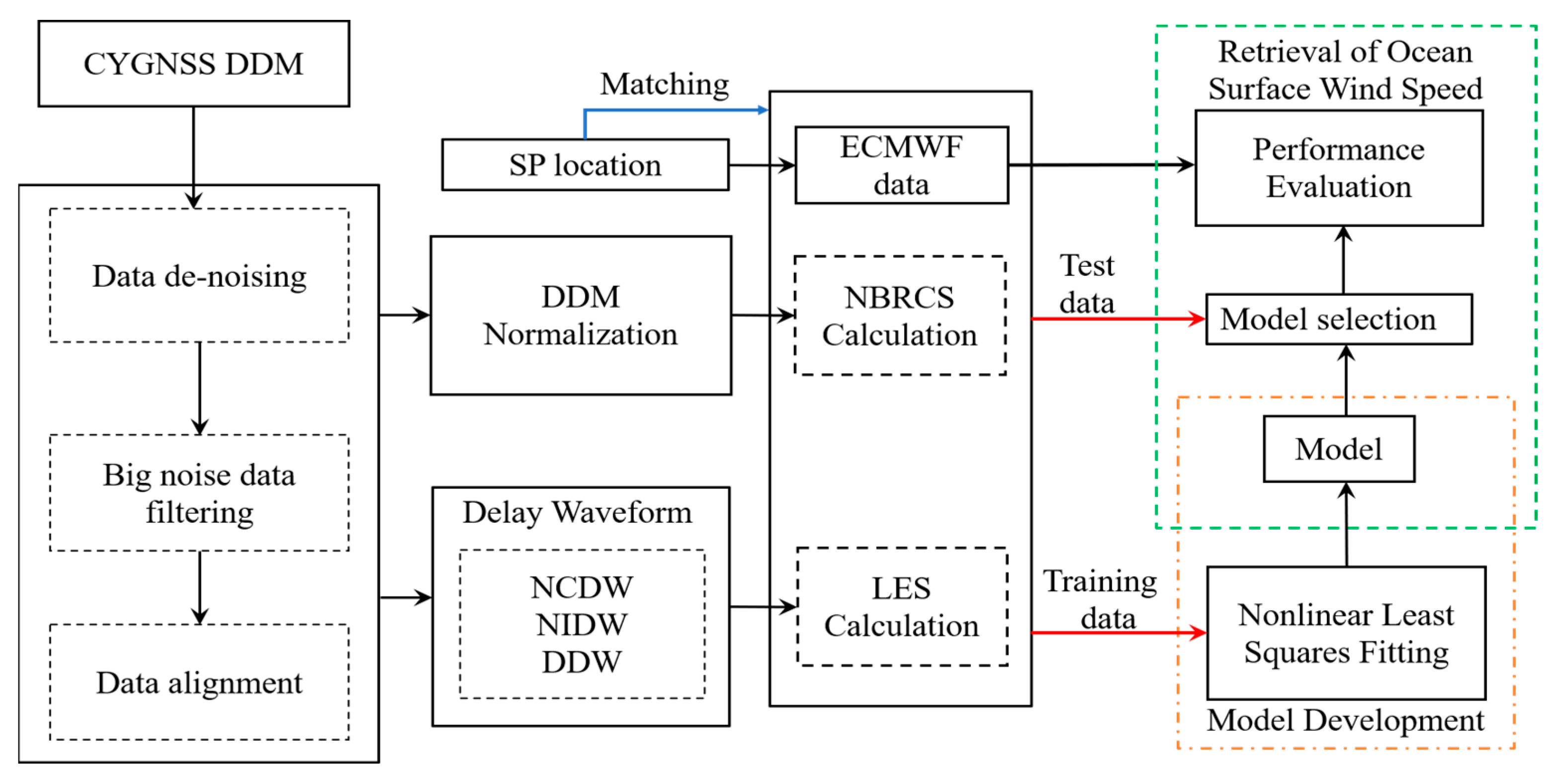
Some researchers proposed and improved the calculation method of NBRCS [56,57,58]. Combined with power calibration, NBRCS can be calculated more accurately, so it can be well suited for the typical sea-surface wind speed range. In Jing et al. [30], an empirical model of geophysical function was developed based on DDM data and NBRCS observations obtained by BF-1 satellite. The results showed that the RMSE of the model-based estimation using the ECMWF data as the ground truth was 2.63 m/s, with a determination coefficient of 0.55. Bu et al. [59] proposed a combined model for wind speed retrieval by using NBRCS and LES observables. Figure 1 shows the flowchart of the CYGNSS data-based wind speed estimation method proposed in [59]. The RMSE of the combined method was 2.1 m/s and the determination coefficient was 0.906. Compared with the method based on single NBRCS and LES, it achieved considerable performance gain.
Although a lot of work has been conducted on ocean wind speed estimation based on spaceborne GNSS-R DDM observables, such as DDMA, LES, and TES, further research is needed to develop wind speed estimation models using NBRCS observables. Pascual et al. [60] improved the wind speed estimation method using significant wave height (SWH) as an external source of reference data. The results showed an increased sensitivity to large wind speeds, with a reduction in the root-mean-square difference (RMSD) from 2.05 m/s to 1.74 m/s when using the ECMWF wind data as a reference.
In recent years, the GNSS-R wind speed retrieval algorithm has been significantly improved, and has opened a window for retrieving global wind speed from spaceborne GNSS-R data. However, thus far, only a limited set of observables and features have been utilized in algorithm development. To establish a more comprehensive and accurate wind retrieval model, it is useful to use a deep-learning-based GNSS-R algorithm to measure global ocean wind speed [61,62,63]. Deep learning offers the capability of correcting the effects dictated by the data. In future, samples within a larger wind range should be selected for a widely applicable GNSS-R wind retrieval model.
2.2. Sea Surface Significant Wave Height Estimation
A sea wave is generated by local sea surface winds, and is a wind-driven wave. It can also be generated by long-distance storms, which are called swells. In many cases, a sea wave consists of local wind-driven waves and swells. It is affected by a range of factors including wind speed, wind direction, and terrain. The sea-wave height fluctuates greatly, usually from a few centimeters to several meters, mostly depending on the wind speed. Observing the distribution of wave height on a global scale is one of the key research areas in oceanography [64]. Wave height is usually measured by significant wave height (SWH) which is defined as the average height of the largest one-third of waves in the spectrum [65]. SWH observations are very important for the study of the assessment of wave energy resources and the prediction of ocean storm disasters. Satellites and buoys are commonly used to observe sea surface SWH for coverage and accuracy assessments. For instance, since 1970, satellite radar altimeters have been used for global SWH measurement, such as Jason-1 and Jason-2 [66]. Additionally, synthetic aperture radar (SAR) techniques can be used to measure SWH with an accuracy of 0.32 m in terms of root-mean-square error [67]. Although these techniques have high accuracy of observations, they can only sense the narrow surface swath underneath the satellite, and the time resolution of the observations is low. For buoys, they have higher accuracy of observations and high temporal resolution, but they are limited by number and cost, and can only observe a small area near the coast [68]. Therefore, it is challenging to estimate SWH with high temporal and spatial resolution on a global scale.
Compared with traditional remote sensing technologies, spaceborne GNSS-R technology is cost-effective, and in the presence of multiple sensors such as CYGNSS, which consists of multiple spatially distributed micro-satellites, it has higher spatial resolution with global coverage compared with the European Centre for Medium-range Weather Forecast Reanalysis 5th Generation (ECMWF ERA5) SWH data. There are very few studies on spaceborne GNSS-R technology for SWH estimation, and only a preliminary understanding of this topic can be obtained based on the rather limited literature. Peng et al. estimated SWH by using the CYGNSS DDM data, and verified the feasibility of estimating SWH using spaceborne GNSS-R technology [69]. The ECMWF ERA5 SWH data was used as the ground-truth data. Inspired by the SWH measurement formula of X-band radar [70], they used the SNR of DDM to estimate SWH.
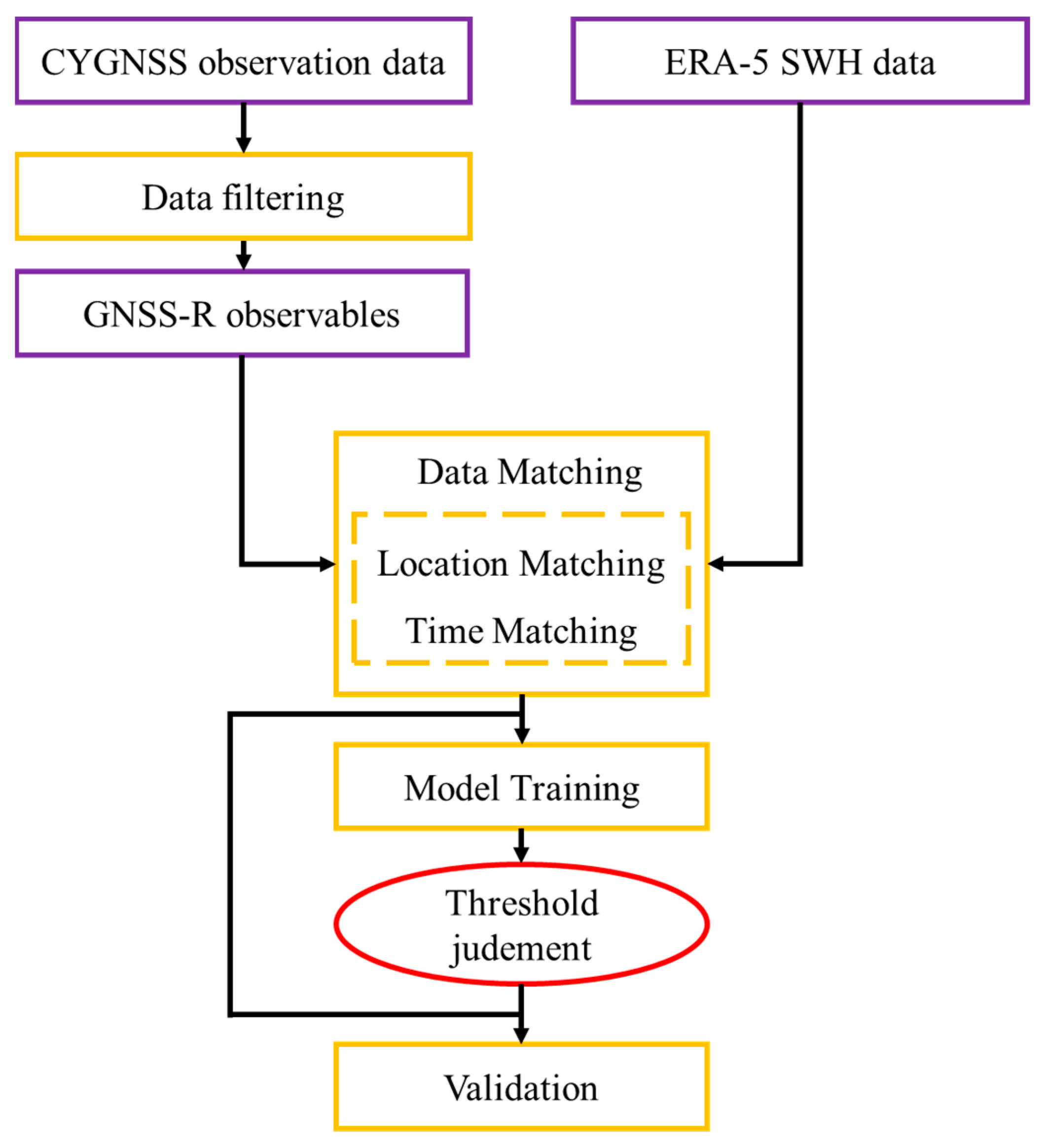
Many studies have demonstrated the ability of DDMA (delay–Doppler map average) and leading-edge slope (LES) in retrieving the physical parameters of the reflecting sea surface, both of which can be generated from DDM data [36,46,61]. Yang et al. [71] made some further modifications to the method presented in [69]. They constructed a polynomial function model for estimating SWH by using the DDMA and LES, and obtained better results. After that, Bu and Yu [72] developed a geophysical model function (GMF) for SWH retrieval based on the spaceborne GNSS-R data measured by the CYGNSS satellites. Four GNSS-R observables (i.e., the leading-edge slope (LES) of the normalized integrated delay waveform (NIDW), the LES of the normalized central delay waveform (NCDW), the trailing-edge slope (TES) of the NCDW, and the leading edge waveform summation (LEWS) of the NCDW) derived from DDM are used to retrieve SWH. The results showed that there was high consistency between the SWH estimates and the ERA5 SWH data, with a correlation coefficient of 0.88 and an RMSE of 0.503 m. Generally speaking, the main ideas of the current research on the estimation of SWH are basically the same, although the main difference is that the proposed models are different; the calculation process is shown in Figure 2. In fact, the current technique of SWH estimation on spaceborne GNSS-R technology has limitations, and can only be applied to specific days or areas. Thus, further research is needed in the future.
3. Spaceborne Rainfall Detection and Rainfall Intensity Retrieval
Rainfall detection (RD) and rainfall intensity (RI) retrieval are focused on hotspots in ocean remote sensing. In recent years, the research on RD has mainly been based on X-band ocean radar images. When retrieving other parameters such as ocean wind speed and effective wave height, rainfall is usually considered as interference; thus, only images less disturbed by rainfall are retained in radar image processing, and images with serious interference are ignored [73]. A number of methods for RD have been proposed by scholars, including the zero-pixel percentage (ZPP) method [74], the support vector machine (SVM) method [75], the correlation characteristic difference method [76], and the ratio of zero intensity to echo (RZE) method [77].
RI can be used as an index to judge the reliability of retrieved wind and wave information. If the RI is high, the retrieved wind and wave information cannot be credible if the effect of rainfall is not suppressed. In the absence of rainfall interference or low RI, the retrieved wind and wave information is credible [76,77]. In addition, RI is one of the key parameters of precipitation information in meteorological observations, and has important implications in weather forecasting, climate change studies and aviation flight safety. The spatial and temporal changes in RI also have important effects on atmospheric cycle, ecological governance, and hydrological calculations [78,79,80]. At present, RI measurement mainly relies on traditional rain gauges and remote-sensing sensors [81,82,83]. A rain gauge can only measure rainfall at a certain location, and only reflects the RI of an area around that location; the application of remote sensing technology can greatly expand its measurement range [84,85]. At present, the research on RI retrieval is mainly based on X-band ocean radar images. For example, Lu and Zhang et al. extracted parameters such as frequency reflectance in the wavelet domain using zero intensity percentage and stationary wavelet transform methods for RI inversion [77,86]. In recent years, deep learning has also been applied to rainfall retrieval [87,88], with satisfactory experimental results.
With the development of meteorological satellites, in recent years, a lot of research results have been obtained using satellite remote sensing to retrieve rainfall products [89,90,91]. At present, some open source rainfall products can be widely used in hydrology, meteorology, environmental science and other fields; these include the Climate Prediction Center MORPHing (CMORPH); Tropical Rainfall Measuring Mission (TRMM); Multi-satellite Precipitation Analysis (TMPA); Precipitation Estimation from Remotely Sensed Information using Artificial Neural Networks (PERSIANN); IMERG (Integrated Multi-Satellite Retrievals for Global Precipitation Measurement); TRMM-3B42V7, GSMaP (Global Satellite Mapping of Precipitation); CHIRPS (Climate Hazards Group InfraRed Precipitation with Station); ERA5; ERA Interim (ECMWF Reanalysis Interim); and SM2Rain-ASCAT (Advanced SCATterometer) [80,92,93]. Some scholars have analyzed and compared these rainfall products, and the results show that IMERG has the best performance in rainfall estimation [80,93,94].
To sum up, although many studies have discussed the use of radar and satellite remote sensing techniques for RD and intensity estimation, and many useful results have been obtained, few techniques have considered the requirements of cost, revisit cycle, and spatial resolution at the same time. As discussed in the preceding sections, GNSS-R has been applied to ocean remote sensing.
GNSS-R shows great potential due to its advantages of low observation cost and abundant signal sources. Additionally, as mentioned earlier, the UK, US and China successfully launched TechDemoSat-1 (TDS-1) [38], Cyclone Global Navigation Satellite System (CYGNSS) [27] and BuFeng-1 A/B satellites in 2014, 2016 and 2019 [30], respectively. In addition, there are FSSCat [51,95,96,97] and TRITON [53,98,99,100] satellite missions dedicated to GNSS-R applications. Although this technique has been successfully applied to the retrieval of various geophysical parameters [21,101,102,103,104,105,106], research using the technology to obtain rainfall information is very limited. There have been some preliminary studies on the effects of rainfall on GNSS-R altimetry and ocean wind measurements [107,108,109,110,111]. Rainfall features were observed in TDS-1 L1B DDM data [108], confirming, for the first time, the possibility of spaceborne GNSS-R rainfall observations. Asgarimehr et al. [110] studied the effect of rainfall signal attenuation on a bistatic radar cross section and wind speed retrieval. The results show that atmospheric attenuation by raindrops is insignificant in the spaceborne GNSS-R L-band measurements. However, the influence of rainfall on sea surface roughness can be significant, and extra local winds (mainly downdrafts) caused by rainfall can also be significant. Balasubramaniam and Ruf [111] also studied rainfall characteristics using CYGNSS L1B DDM data and gave a similar explanation for the rainfall effect at low wind speed.
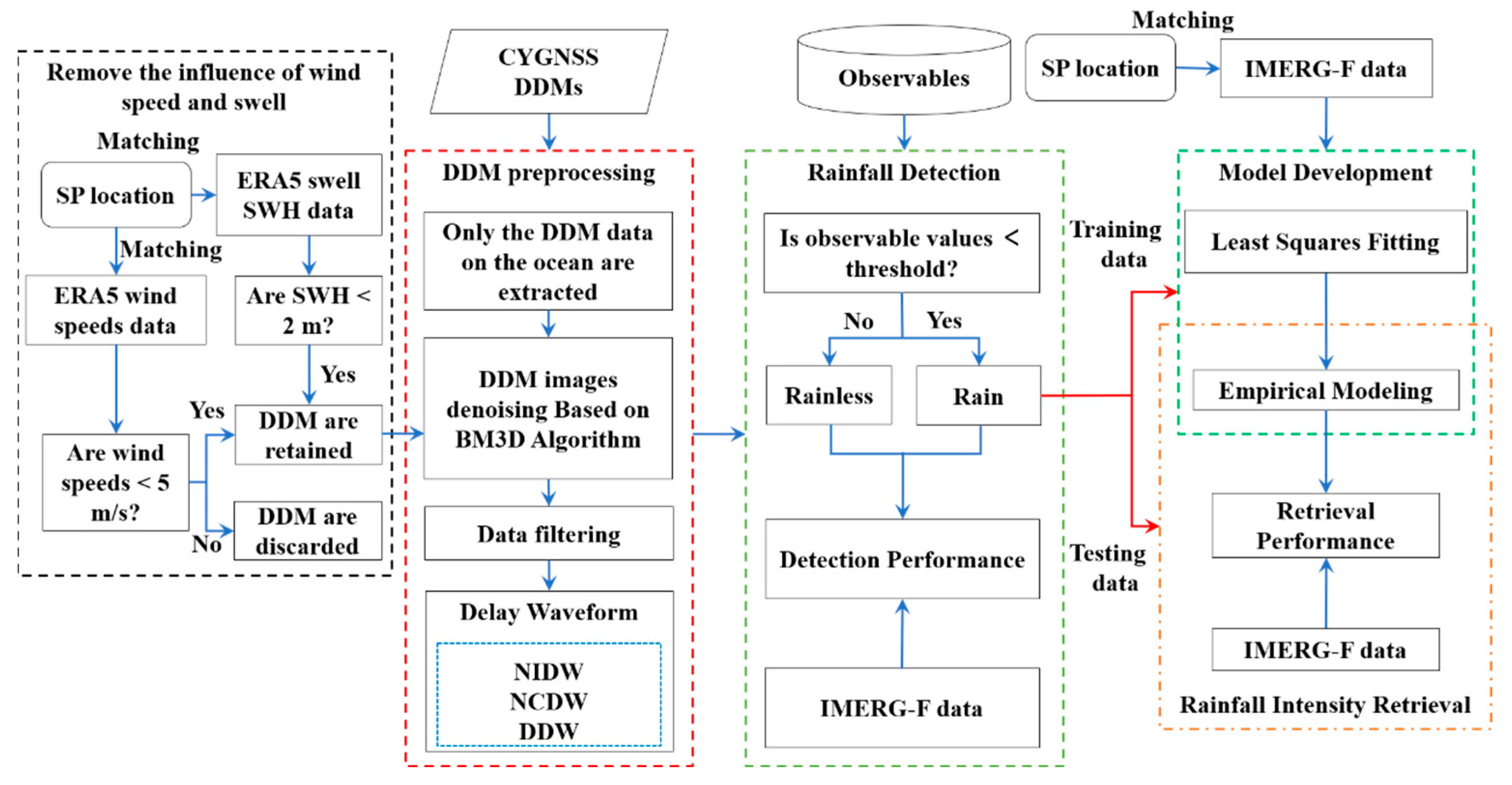
Although preliminary studies on the effect of rainfall on GNSS-R ocean wind measurements are reported, no further work has been carried out on RD and RI retrieval. To further understand the interaction between rainfall and the air–sea interface and its impact on GNSS-R measurements, more research on the retrieval of RD and RI is necessary. Motivated by such an observation, Bu and Yu [112] conducted a preliminary study on sea surface RD and RI retrieval using spaceborne GNSS-R technology. They proposed the RD and RI retrieval algorithm as described in Figure 3. The experimental results showed that under very low wind speed (<5 m/s) the proposed trailing edge waveform summation of the normalized integral delay waveform (TEWS-NIDW), the TEWS of the normalized center delay waveform (TEWS-NCDW), and the TEWS of the differential delay waveform (TEWS-DDW) observables were more suited for RD, and the probability of detection of rainfall (PDr) was better than 75%. The mean square errors (MSE) of RI retrieval for the 12 observables considered were all less than 4.66 mm/hr, with the model based on the TEWS-NCDW observable achieving the highest accuracy, at better than 3.74 mm/hr. However, DDM observations are only very sensitive to rainfall at low wind speeds (<5 m/s), above which DDM observations may be greatly affected by wind speed, leading to rainfall information being easily obscured by wind speed. Thus, the study only focused on sea surface RD and intensity retrieval when the wind speed was lower than 5 m/s. In the presence of medium and high wind speeds and large swells, whether it is possible to use the spaceborne GNSS-R technology for sea surface RD and RI retrieval still needs further investigation.
4. Spaceborne Sea Surface Altimetry and Land Topography
4.1. Sea Surface Altimetry
The characterization of sea level height has always been important to human beings. The variation in sea level on a global scale is probably caused by climate change. The sea level increase results in more frequent flooding and reduces the land size of many islands and coastal areas. Recently, sea level measurement using GNSS-R technology has become a research hotspot. Martin-Neira [5] first proposed the use of spaceborne GNSS-R to measure sea levels in 1993. The main objective was to develop a passive reflectometry and interferometry system (PARIS) in a low Earth orbit to densify sea-level measurements from a radar altimeter. Since then, many studies for sea-level measurements based on GNSS-R have been carried out at different observation heights and platforms, e.g., spaceborne, airborne, and ground-based platforms. Compared with ground-based and airborne measurement methods, spaceborne GNSS-R has provided a new opportunity to measure sea levels with a global coverage.
With the gradual maturity of ground-based GNSS-R and airborne GNSS-R technologies, there have been more investigations on the use of spaceborne GNSS-R in ocean altimetry. Clarizia et al. [113] used spaceborne GNSS-R data from the TDS-1 satellite to retrieve the sea surface height (SSH), and the results were in general agreement with the global DTU10 mean surface height; this was the first spaceborne GNSS-R altimetry study. Li et al. [114] performed phase altimetry over sec ice using TDS-1 satellite data and showed good agreement with a mean sea surface (MSS) model with a root-mean-square difference of 4.7 cm. Mashburn et al. [115] investigated the performance of the TDS-1 data for SSH retrievals. Compared with the mean sea surface topography, the surface height residuals were found to be 6.4 m with a 1-s integration time, which proves the potential of spaceborne GNSS-R for SSH measurement. Hu et al. [116] investigated measurement errors due to receiver dynamics and showed that the dynamic of LEO receivers can lead to errors of a few meters, depending on the receiver trajectory angle. Xu et al. [117] first applied spaceborne GNSS-R altimetry to global lake levels, and the measurements showed consistent spatial and temporal variability between TDS-1 data measurements and other data sources. Li et al. [118] assessed the ocean altimetry performance of spaceborne GNSS-R by processing the raw data sets collected by CYGNSS constellation. Compared with the average SSH model, the measurement results showed good consistency. Qiu et al. [119] estimated the global mean sea surface height (MSSH) by using CYGNSS data. Compared with the measurement results of the other three products, a good agreement was obtained.
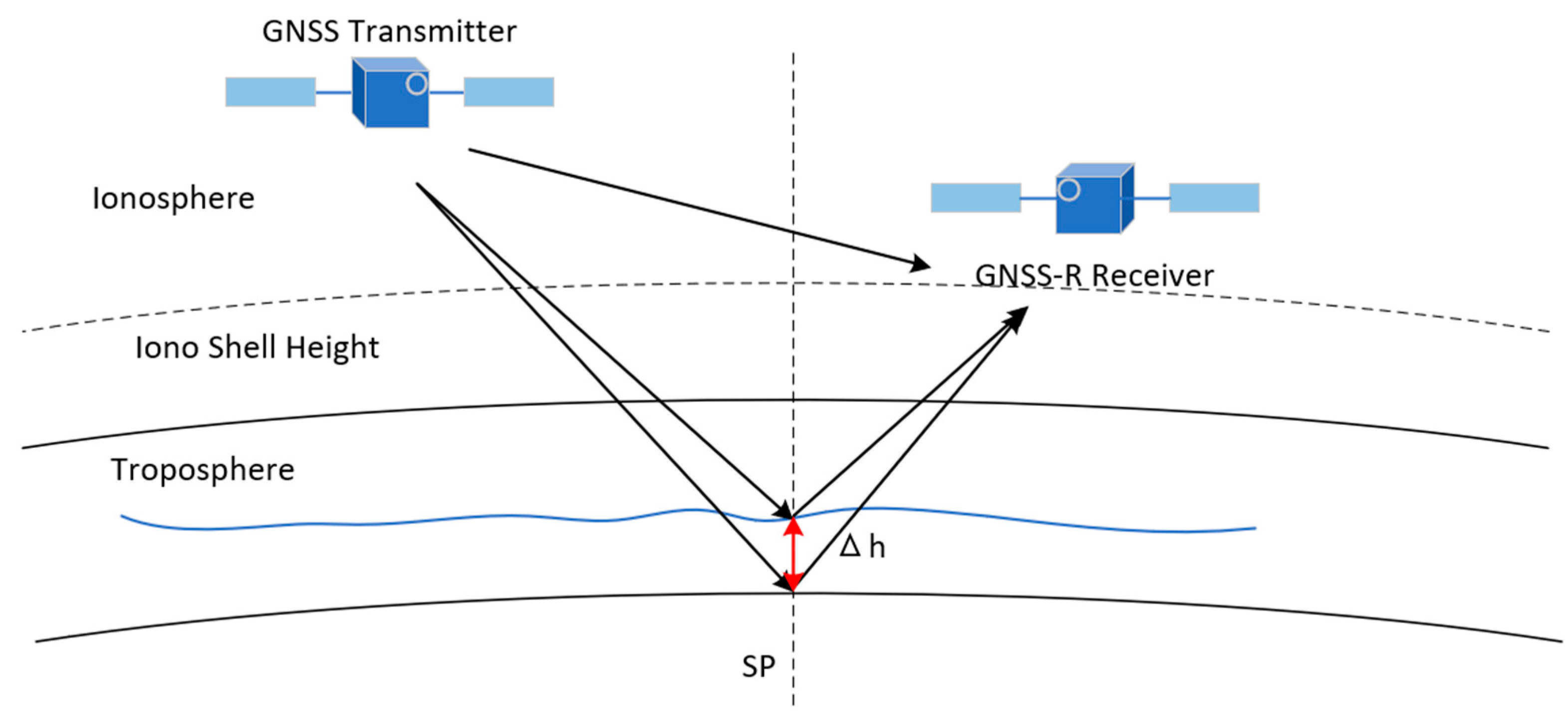
Mashburn et al. [120] presented a reflection-model-based approach for delay retracking and verified it with CYGNSS data collected in Indonesia, which further improved the accuracy of the measurements. Hu et al. [121] studied the validation of the leading-edge derivative (LED) in spaceborne GNSS-R altimetry. Song et al. [122] used two sets of 40 s raw intermediate-frequency (IF) data from TDS-1 to estimate SSH, and the results showed that the accuracy of the code phase altimetry was up to 0.51 m on the sea ice and 13.09 m on the typical sea surface. The geometric model of altimetry is shown in Figure 4, and the compensation of ionospheric delay and tropospheric delay also needs to be deeply studied. Zhang et al. [123] investigated the effect of the ionosphere on spaceborne altimetry and analyzed the optimal value of spatial filtering to eliminate the ionospheric delay in altimetry. Cardellach et al. [124] used the GA carrier phase of the GPS and Galileo signals from the CYGNSS data for altimetry, and the results showed that the measurement precision was 3 cm/4.1 cm (median/mean) at a sampling rate of 20 Hz. Centimeter precision was achieved at a sampling rate of 1-Hz, which is comparable to dedicated radar altimeters. The combined precision, including systematic errors, was 16 cm/20 cm (median/mean) with a 50-ms integration time, and a few centimeters with a 1-Hz sampling frequency. Wang et al. [125] proposed a simultaneous cycle-slip and noise-filtering (SCANF) method that can be used as dual-frequency GNSS-R phase measurements generated by OL tracking, and tested its performance using real phase measurements from Spire’s low Earth orbit (LEO) satellites. The average root mean square of the retrieved sea surface height anomaly (SSHA) retrieved using reflections on the sea surface and sea ice surface was 7.3 cm, compared to the mean sea surface (MSS). Cui et al. [126] established a dual circularly polarized phased-array antenna (NDCPPA) model of an iGNSS-R (interferometric GNSS-R) measurement system based on the theory of coherent signal processing for signals reflected over the sea surface. The results showed that, compared with the TEA method, the antenna gain of this model was increased by 9.5 dB and the altimetric precision of the nadir point was improved from 7.27 m to 0.21 m.
In summary, the research on spaceborne GNSS-R altimetry mainly focuses on the theoretical studies and performance evaluation based on existing spaceborne platforms. There are fewer data available for spaceborne GNSS-R altimetry, and more data sets or products are required. As the current spaceborne instruments (such as TDS-1, CYGNSS) were mainly designed for specific GNSS-R applications such as sea-surface wind speed retrieval. There are still certain problems when using spaceborne GNSS-R satellites for altimetry—such as accurate orbit information, and ionospheric and tropospheric delay corrections—which add uncertainty to the measurements and mask their true accuracy. The commonly used altimetric method is cGNSS-R (conventional GNSS-R) code phase altimetry based on the DDM delay waveform, which is less accurate due to the limitations of the method itself and the lack of satellite position and other information. The iGNSS-R carrier-phase altimetry method can achieve high accuracy in measurements, but requires IF data; however, a rather limited number of satellite-based IF data are provided. For instance, three sets of 40 s IF data are available for TDS-1, and a relatively larger number of IF data are available from CYGNSS. In the future, more research will focus on spaceborne altimetry, including topics on the dedicated design of spaceborne receivers, altimetry error correction, altimetry methods, and more applications based on altimetry.
4.2. Land Topography
The retrieval of topographic parameters based on GNSS-R is also a new research topic. Carreno-Luengo et al. found that there is a functional relationship between DDMs from CYGNSS and several topographic parameters from a digital elevation model (DEM) [127]. They employed a target area in South Asia to observe the surface curvatures. The results showed that the trailing edge and reflectivity were strongly correlated with the topographic wetness index. At nearly the same time, the effects of rough topography on GNSS-R observations were studied in [128]. The results showed that the terrain ruggedness index and profile curvature had a moderate-to-strong impact on the CYGNSS-derived trailing edge and reflectivity at low elevation angles. Later, Campbell et al. [129] developed a model to describe the effects of topography on delay–Doppler maps. Wang et al. [130] made use of GNSS-R for land surface altimetry applications. They processed the CYGNSS raw IF data using adaptive hybrid tracking. They also studied a semi-coherent land-reflection event over Vietnam and a coherent reflection pass over the Orinoco River, and the results demonstrated pseudorange-based land altimetry at meter-level accuracy, and inland water-body surface-height retrieval at centimeter-level precision. The current research demonstrates the feasibility of the spaceborne GNSS-R inversion of land topography; however, related studies are relatively few and in the exploratory stage, and there is much space for future development.
5. Spaceborne Retrieval of Soil Moisture and Vegetation Parameters
5.1. Soil Moisture Estimation
Soil moisture, one of the important indicators for forecasting droughts and floods and estimating crop yields, and has very important implications for energy exchange between the land and atmosphere, as well as the global water cycle. Soil on a global scale is of great value for weather forecasting, climate change study, and the monitoring of extreme weather events.
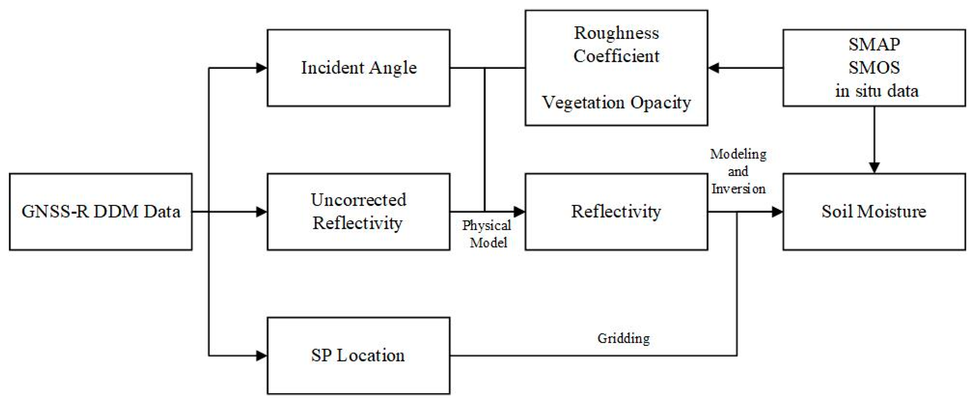
The basic principle of spaceborne GNSS-R soil moisture inversion is to use the sensitivity of reflectivity of the reflected signal to soil moisture, and its inversion process is shown in Figure 5. Recently, because of its advantages such as abundant signal sources and low cost, many scholars have started to use spaceborne GNSS-R technology to invert soil moisture with Soil Moisture Active–Passive (SMAP), Soil Moisture and Ocean Salinity (SMOS) or in situ data as the ground-truth data, which has made considerable progress. Camps et al. [131] explored the sensitivity of TDS-1 GNSS-R data to soil moisture, and by considering different vegetation covers, they developed a vegetation correction model for reflectance based on the Tau-Omega model. Chew et al. [132] used TDS-1 data to calculate the coherent component of the signals to retrieve soil moisture, and a 7 dB sensitivity of reflected signals to temporal variation in soil moisture was observed. Camps et al. [133] used different observations to retrieve soil moisture, and it was shown that the sensitivity of the calibrated GNSS-R reflectivity to soil moisture was ~0.09 dB/% when the incidence angle was up to 30°. The reflectivity decreased with an increased incidence angle, although the variations depended on the location and the spatial scale used for the ground-truth data. Carreno-Luengo et al. [134] evaluated the influence of the GNSS satellites’ elevation angle on reflectivity. The results showed that the smoother the land surface, the greater the angular variability of the Pearson correlation coefficients. Kim et al. [135] introduced the concept of relative SNR, which provides useful soil moisture estimates over moderately vegetated regions. Ban et al. [136] proposed two new approaches—GEO-IR and GEO-R—for soil moisture retrieval using geostationary satellite signals. The results showed that the proposed GEO-IR and GEO-R were able to monitor soil moisture reliably under bare soil conditions, augmenting GNSS-R through significantly reduced processing complexity and increased temporal coverage. Calabia et al. [137] investigated the retrieval of soil moisture content from CYGNSS data by estimating the dielectric permittivity from Fresnel reflection coefficients. The estimates of soil moisture content had an R-square of 0.6, an RMSE of 0.05 m3/m3, and a p-value of zero. Wan et al. [138] used BuFeng-1 A/B data of the first Chinese GNSS-R mission for soil moisture inversion, and the results were in good agreement with the soil moisture data generated by SMAP (correlation coefficient of 0.94 and RMSD of 0.029 m3/m3) as well as with in situ data (correlation coefficient of 0.77 and RMSD of 0.049 m3/m3. Senyurek et al. [139] evaluated the spatial interpolation error in soil moisture retrieval and the results indicated that the overall interpolation error in terms of RMSE was 0.013 m3/m3 over SMAP’s recommended grids.
Most studies have considered the coherent component of the reflected signal, while some scholars have studied the effect of the incoherent component on soil moisture retrieval. Al-Khaldi et al. [140] considered the incoherent scattering from the land surface and performed a time series inversion of soil moisture using CYGNSS satellite data. The results suggested the potential of spaceborne GNSS-R systems for global soil moisture retrieval with an RMSE on the order of 0.04 cm3/cm3 over varied terrain. Dong et al. [141] proposed and tested a detection method to separate the coherence of land GNSS-R DDM, and evaluated the impact of coherence on the inversion. The results showed that the incoherent components had little effect on the soil moisture retrieval, and the accuracy of GNSS-R soil moisture inversion was 0.04 cm3/cm3.
Recently, machine learning methods have been widely used in various research directions, and many scholars have combined machine learning methods with spaceborne GNSS-R for soil moisture inversion [142,143,144,145,146,147,148]. For example, Eroglu et al. [142] used a fully connected Artificial Neural Network (ANN) to invert soil moisture by learning the nonlinear relationship between the CYGNSS observables and the soil moisture, as well as other land geophysical parameters. At a spatial resolution of 0.0833° × 0.0833°, the ubRMSE (unbiased RMSE) of the soil moisture retrieval was 0.0544 cm3/cm3 with a correlation coefficient of 0.9009. Jia et al. [143] used the XGBoost method to analyze the performance of the input features, which helped to further understand the GNSS-R soil moisture inversion. Senyurek et al. [147] used three machine learning methods (ANN, RF and SVM) to retrieve soil moisture, and a variety of verification strategies were used for comparison and analysis; these indicated that the model, built based on the machine learning approach, had higher accuracy and could be generalized in the space and time domains. In 2021, Jia et al. [148] used machine learning regression aided by a pre-classification strategy, which achieved a measurement accuracy of 0.052 cm3/cm3 in terms of RMSE. Many machine learning methods are flexible and capable of dealing with non-linear problems. They can tap into the complex interactions between inputs and outputs and build models that ultimately make good predictions, and have shown promising results in soil moisture inversion.
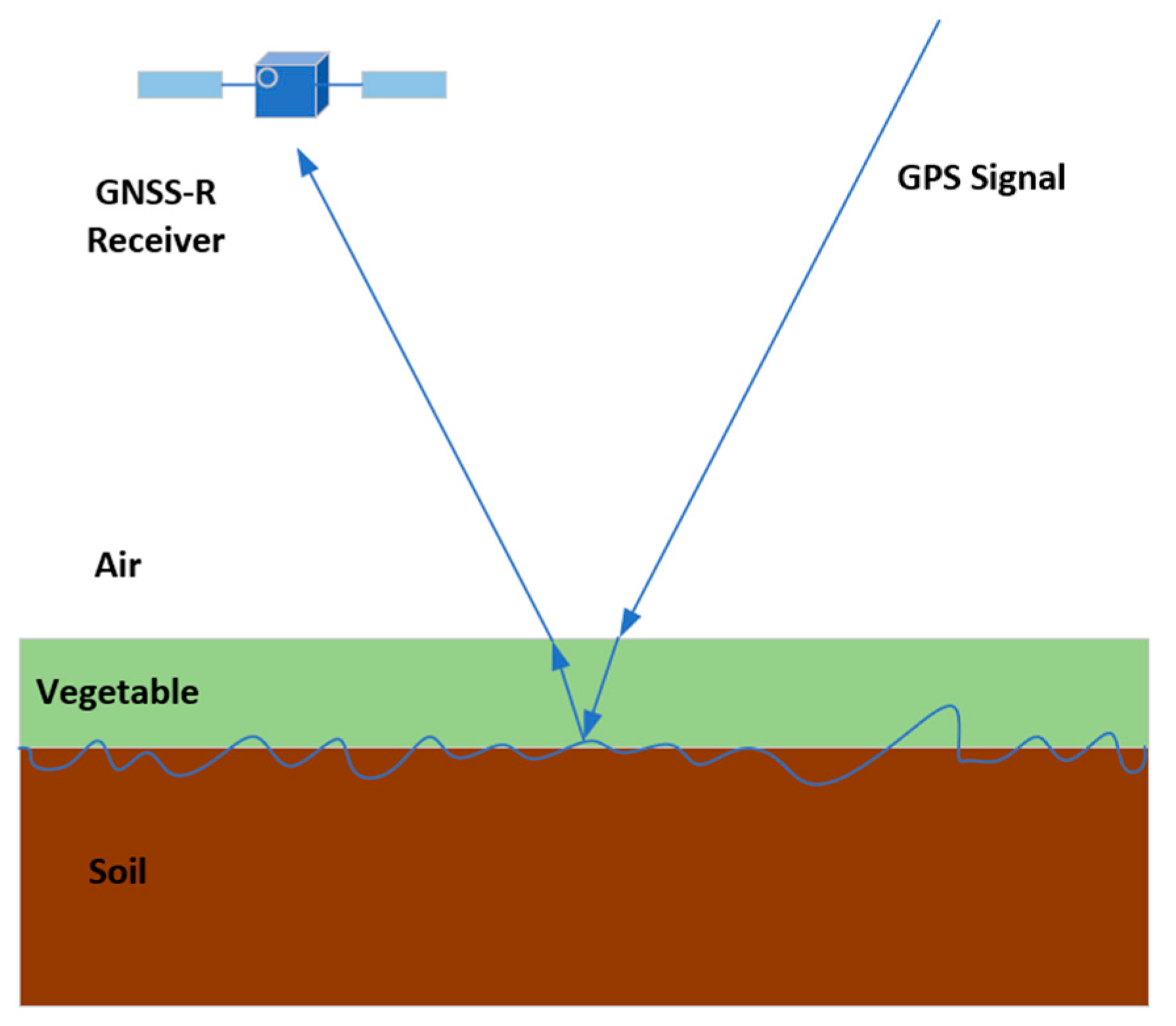
Overall, a large number of research results are available for spaceborne soil moisture inversion, which demonstrates the feasibility of spaceborne GNSS-R in soil moisture measurement. However, some issues still need to be studied in depth to achieve possible performance enhancement. For instance, there are uncertainties in the data related to factors such as receiver gain, satellite transmission power and, in some cases, antenna gain. In addition, the error in estimated receiver position can lead to errors in the calculation of specular points [142]. Additionally, the inversion process is highly dependent on auxiliary data such as vegetation, surface roughness and incidence angle, which are often ignored [131,132,137,147] or normalized [140,149,150]. Roughness and vegetation effects are usually compensated using physical models. For example, as shown in Figure 6, for a flat and smooth area covered by vegetation, the surface reflectivity Γ can be modeled as [151,152]:
where , , and are the incident angle, Fresnel reflection coefficient, and transmissivity, respectively, and the transmissivity indicates the attenuation of the signal propagation by vegetation. The parameters and in the exponential term represent the signal wavenumber and the surface root-mean-square height, respectively, indicating the effect of roughness. It is still useful to investigate more appropriate ways to remove or compensate for the effects of those parameters. Furthermore, only coherent components are considered in most of the existing literature, and how to deal with coherent and non-coherent components at the same time remains to be further investigated [153].
5.2. Vegetation Monitoring
As an important component of terrestrial ecosystems, vegetation plays an important role in the global carbon cycle. Traditional remote sensing methods such as optical and thermal infrared remote sensing have some limitations in vegetation monitoring, and the development of GNSS-R provides a new supplementary method for vegetation monitoring. The pioneering experiments of ground-based GNSS-R [3,154,155,156,157,158] and airborne GNSS-R [159,160,161,162,163] have proved the potential of GNSS-R remote sensing technology in vegetation monitoring. Due to the launch of spaceborne missions (e.g., CYGNSS and TechDemoSat-1), scholars started investigating vegetation monitoring based on spaceborne data. By utilizing TDS-1 data, Camps et al. [131] analyzed the sensitivity of soil moisture on different ground surfaces (i.e., vegetation covers) and a large-scale NDVI (Normalized Difference Vegetation Index) to GNSS-R scattering energy. The results indicated a great sensitivity of NDVI to soil moisture and a good correlation coefficient for low NDVI values, which shows the feasibility of vegetation monitoring using spaceborne GNSS-R.
Carno-Luengo et al. [164] conducted the first GNSS-R experiment on a global scale, performed on-board the SMAP (Soil Moisture Active–Passive) satellite, to study soil moisture and biomass retrieval. The scattered GPS L2 signal was received by the SMAP’s dual-polarization (Horizontal and Vertical) radar receiver. By setting the optimum coherent integration time of 5 ms, the DDM data were obtained through signal processing. The SNR, the Polarimetric Ratio (PR), and the width of the waveforms’ trailing and leading edges were used to analyze the Earth’s topography and Above-Ground Biomass (AGB). By comparing the soil moisture retrieved by GNSS-R and the soil moisture obtained by the SMAP radiometer, consistency was obtained with a linear correlation coefficient of 0.6. The mean SNR of H-polarization was different for different terrain types. The waveform-derived parameters showed sensitivity to seasonally changing geophysical parameters, i.e., the NDVI and SWI (Soil Water Index). The spreading of the waveforms’ LES and TES decreased when AGB values were increased from 100 ton/ha to 350 ton/ha. AGB was more sensitive to GNSS-R signatures (PR, SNR, LES and TES) than the NDVI. It was determined that GNSS signals will depolarize in areas with rough ground or high AGB values.
Carno-Luengo et al. [165] simulated the relationship between GNSS-R observations and a forest biomass of rain, coniferous, dry, and moist tropical forests using CYGNSS data. The AGB map and the forest canopy height data of ICESat-1/GLAS data were selected as the biomass reference datasets. The results of the polynomial regression showed that TES and reflectance will decrease when the biomass (~400 ton/ha) increases. Intervals of 10° were set to analyze the influence of elevation angles on biomass retrieval. By analyzing the relationship between reflectivity and TES, and biomass at different elevation angles, they claimed that biomass retrieval is affected by elevation due to different scattering mechanisms. The influence of surface scattering and volume scattering on TES and effective reflectivity in different kinds of biomass were also considered.
Santi et al. [166] studied the capability of spaceborne GNSS-R in evaluating forest biomass using data from the TDS-1 mission and the CYGNSS mission. They used the corrected DDM peak to retrieve an equivalent reflectivity and evaluated its sensitivity to forest parameters. The analysis showed that the observed equivalent reflectance decreased when the forest biomass increased. To improve the retrieval accuracy, other inputs (e.g., the incidence angle, SNR, and the lat/lon information) were added to the artificial neural network algorithm, which showed a great ability to retrieve biomass and tree height. The algorithm was tested on both the selected areas and globally, and there was good consistency, with a correlation coefficient of 0.8. The dDM peak comprised both specular and diffuse scattering, and its sensitivity to forest parameters was considerable. However, the TDS-1 had limited coverage and CYGNSS data was limited to the central latitudes.
6. Spaceborne Sea Ice Detection and Sea Ice Thickness Estimation
6.1. Sea Ice Detection
GNSS-R technology was first used for sea ice detection in 2000, when Komjathy et al. [167] compared the peak power of the waveform of the reflected signals from the ice surface with the RADARSAT backscattered echoes. Wiehl et al. [168] studied the possibility of using GNSS-R techniques for ice sheet sensing and developed a theoretical model demonstrating the scattering mechanism of the ice sheet. Then, the shape of the reflected GPS signals delay waveform was analyzed and the permittivity and roughness of the different types of sea ice were investigated [169]. With the successful launch of the United Kingdom Disaster Monitoring Constellation (UK-DMC) in 2003, spaceborne GNSS-R was firstly used for sea ice sensing by Gleason [170], and more details were presented in [171]. In a study of ice altimetry, [172] made use of ground-based GNSS-R experiments, and theoretically exploited the coherent differential phase between direct and both cross- and co-polar reflected signals. Two additional sea ice detection methods based on ground-based experiments are described in [173]. Later, the ground-based GNSS-R sea ice concentration was retrieved using the data collected over Bohai Bay. [174].
TechDemoSat-1 (TDS-1), launched in 2014, recorded datasets in the Arctic and Antarctic region, offering the possibility of spaceborne GNSS-R sea ice detection [175]. The TDS-1 data have been successfully applied to sense sea ice parameters over the past few years. Sea ice detection using spaceborne GNSS-R was initially presented by Yan and Huang [176] by calculating the pixel number of each DDM; this is one of the most important GNSS-R observables for demonstrating power scattering from the reflected surface as a function of time delays and Doppler frequencies. Later, Zhu et al. [177] further extended the method using the pixel number and power summation of differential DDM to distinguish ice–water transitions. Schiavulli et al. [178] proposed an alternative method for detecting ice–water transitions based on the analysis of radar image reconstructed from DDMs. The sea ice detection was demonstrated by Alonso-Arroyo et al. [179] by comparing the shape of a theoretical and measured waveform extracted from DDMs. This method achieved a probability of sea ice detection of 98.5%, a probability of false alarm of 3.6%, and a probability of error of 2.5%. This concept can be made computationally efficient by exploiting the temporal correlations of DDMs [180,181]. To establish the theoretical DDM shape, there are several GNSS-R simulators that can be used [18,182,183]. Another study has proven that spaceborne GNSS-R can be effective for sea ice discrimination with a success rate of up to 98.22% compared to collocated passive microwave sea ice data [184]. Two features extracted from DDMs were combined by Cartwright et al. [185] to detect sea ice, with an agreement of 98.4% and 96.6% in the Antarctic and Arctic regions when compared against the European Space Agency Climate Change Initiative sea ice concentration product. Moreover, TDS-1 data were expanded to altimetry applications [114,186]. The ice sheet melt was also investigated in [187] using TDS-1 data. Furthermore, it has been shown that spaceborne GNSS-R is also useful for retrieving sea ice thickness [188] and sea ice concentration [189], which will be further discussed later.
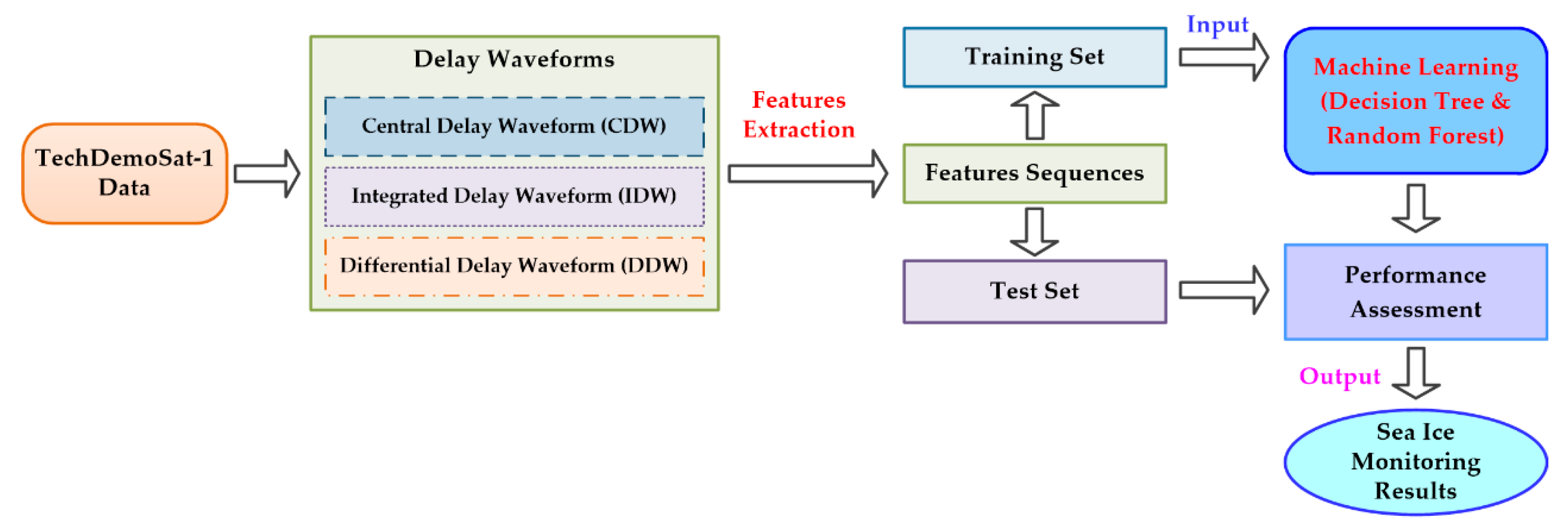
With the development of artificial intelligence, machine-learning (ML)-based methods have been widely used for earth science and remote sensing applications [190]. ML has been proven to be a powerful tool for applications in various remote sensing fields, such as classification [191,192], object detection [193], and parameter estimates [194]. Yan et al. [104] applied the neural network (NN) method to sense sea ice using TDS-1 DDMs. This study presented the potential of an NN-based approach for sea ice detection and sea ice concentration (SIC) estimation, which was further investigated using the convolutional neural network (CNN) algorithm [195]. The DDMs were directly applied as input variables in the CNN-based approach. A Support vector machine (SVM) achieved better performance in sea ice detection [196] than NN and CNN. These three studies used the original DDM and the observables derived from DDMs as input parameters for monitoring sea ice. Zhu et al. [197] utilized feature sequences that demonstrated the characteristics of DDMs as input features to detect sea ice using the decision tree (DT) and random forest (RF) algorithms. Figure 7 shows the basic flowchart of the machine-learning-based sea ice detection approach. The RF-aided method can distinguish sea ice from water with a success rate up to 98.03% validated with the collocated sea ice edge maps from the special sensor microwave imager/sounder (SSMIS) data provided by the Ocean and Sea Ice Satellite Application Facility (OSISAF).
6.2. Retrieval of Sea Ice Thickness
The state of sea ice is determined by its extent, thickness and volume, so sea ice thickness (SIT) is an important sea ice parameter. SIT is particularly sensitive to the coupling effect of the atmosphere, sea ice and ocean. The thickness of sea ice can affect its movement, deformation, freezing and melting processes, and then feed back into the global climate system. Accurate information of polar sea ice thickness and its change is of practical significance to climate research and human production activities. However, due to the complex environmental factors and physical processes of sea ice, SIT is generally considered to be the most difficult sea ice parameter to retrieve. Conventionally, large-scale SIT data can be retrieved by two methods: (1) measuring sea ice elevation (freeboard) based on the conversion between SIT and freeboard using satellite altimeters such as European Remote Sensing [198], ENVISAT [199], and CryoSat-2 [200]; or (2) microwave radiometry according to the model of brightness-temperature measurement and SIT [201], such as Soil Moisture Ocean Salinity (SMOS) [202] and Soil Moisture Active–Passive (SMAP) [203]. Thanks to the launch of United Kingdom (UK) TechDemoSat-1 (TDS-1) in 2014 [175], which covers a high latitude over 80°, the application of GNSS-R in sea ice sensing has drawn significant attention [176,178,179,186,195]. Compared with traditional methods, GNSS-R SIT measurement does not need a transmitter and has rich signal sources, i.e., satellite signals from multiple GNSS constellations. However, so far, the spaceborne GNSS-R SIT measurement has only been able to retrieve thinner ice (<1 m). In addition, only the TDS-1 mission is capable of performing high-latitude GNSS-R detection, and it stopped providing data updates in December 2018, which also limits the development of GNSS-R SIT measurement.
Zhang et al. [174] conducted a ground-based GNSS-R experiment in Bohai Bay and proposed the concept of the polarization ratio (R-LHCP/D-LHCP) between reflected signals and direct signals, based on the dielectric constant properties of sea ice and the Fresnel reflection coefficient; moreover, they studied the GNSS-R-based measurement of sea ice thickness. Li et al. [114] conducted an experiment in Hudson Bay in 2015 and analyzed the elevation residual, i.e., the difference between the retrieved elevation of the reflecting surface and the mean sea surface. The elevation residual showed good correlation with the collocated sea ice thickness data from SMOS (with the best correlation coefficient of 0.79). Meanwhile, the GNSS signal was found to be mainly reflected at the ice–water interface in the case of an SIT of 20 to 60 cm. However, the lack of orbit position of the limited TDS-1 L0 raw data induced a large orbit error in the measurements. Based on the GPS reflected signals collected from two high-altitude lakes with ice cover during winter of 2017–2018, Mayers and Ruf [204] proposed the theoretical method of carrier-phase altimetry to estimate the drift of the ice cover.
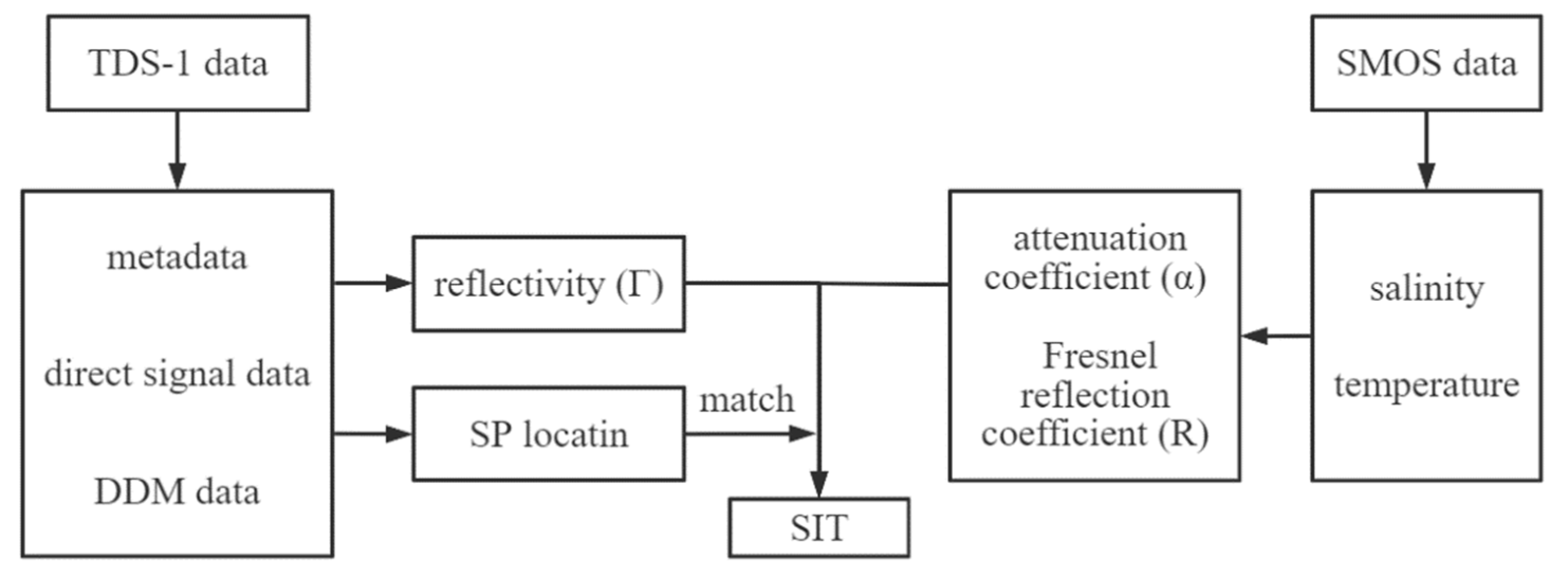
Based on the Fresnel reflection principle and the propagation loss within sea ice, Yan et al. [188] established the relationship between sea ice thickness and reflectivity ():
where and represent the attenuation coefficient over sea ice and the Fresnel reflection coefficient over the ice–water interface, respectively. The SIT calculation process is shown in Figure 8. The calculated SIT (less than 1 m) with (1) and the TDS-1 data were compared with the Soil Moisture Ocean Salinity (SMOS) data. The results showed good consistency between the derived TDS-1 SIT and the reference SIT, with a correlation coefficient of 0.84 and a root-mean-square difference (RMSD) of 9.39 cm.
With the development of machine learning (ML), ML has also been applied to GNSS-R sea ice thickness detection. Two machine-learning methods—specifically, convolutional neural network (CNN) and support vector regression (SVR)—were employed for retrieving SIT from TDS-1 and SMOS data by Yan et al. [205]. Good consistency between the estimated and reference SITs was obtained, with a correlation coefficient of 0.90 and 0.95, and RMSDs of 7.97 cm and 5.49 cm for CNN- and SVR-based methods, respectively; this demonstrates the capability of these machine-learning-based methods and the utility of TDS-1 data for SIT retrieval.
6.3. Classification of Sea Ice Types and Estimation of Sea Ice Concentration
In addition to sea ice detection with TDS-1 data, Yan et al. [205] also made use of NN- and CNN-based algorithms for sea ice concentration estimation. Llaveria et al. [96] used the NN algorithm for sea ice concentration and sea ice extent sensing using GNSS-R data from the FFSCat mission. Rodriguez-Alvarez et al. [206] initially explored the feasibility of the classification and regression tree (CART) algorithm for classifying sea ice types using GNSS-R variables, including the DDM average, leading-edge slope, trailing-edge slope, and generalized linear observable, extracted from GNSS-R DDM. The results demonstrated that the FYI and MYI can be classified with an accuracy of 70% and 82.34%, respectively, based on the comparison with SAR-derived sea ice type maps produced by the US National Ice Center. Zhu et al. [207] used RF and SVM to classify sea ice types based on the feature sequence extracted from GNSS-R observables. Through validation with the data on sea ice type from the special sensor microwave imager/sounder (SSMIS) from the Ocean and Sea Ice Satellite Application Facility (OSISAF), it turned out that the overall accuracy of RF and SVM classifiers were 98.83% and 98.60%, respectively, for discriminating seawater from sea ice, and 84.82% and 71.71%, respectively, for distinguishing FYI from MYI.
7. Spaceborne Flood and Tsunami Detection
7.1. Flood Detection
Floods are one of the most common and destructive natural disasters in the world. Many lives have been lost and great economic loss has been caused due to destructive floods. Optical remote sensing and microwave remote sensing have been widely used in flood monitoring, but they both have advantages and disadvantages. As an emerging remote sensing technology, GNSS-R has been considered for flood monitoring, and would complement the traditional approaches to flood monitoring.
Chew et al. [208] first proposed using spaceborne GNSS-R data for flood detection. CYGNSS data was used to detect flooding in the United States and the Caribbean in 2017, and the results demonstrated that spaceborne GNSS-R technology can provide signals of surface saturation and inundation extent at a higher resolution.
Chew and Small proposed a simple forward model for estimating inundation extent [209]. This model describes the response of surface reflectivity, derived by CYGNSS data, to flooding for different land surface types. They employed the observations from the Amazon Basin and Lake Eyre, Australia, to validate the model. The results showed that surface reflectivity and surface water extent strongly depended on the micro-scale surface roughness of the land and water. In addition, they showed that the dense vegetation surrounding inundated areas had high surface reflectivity due to flooding; moreover, the land surface surrounding the inundated areas was smooth and the surface reflectivity was not greatly increased. Additionally, soil moisture and water roughness have an impact on the detection of surface water. Thus, sufficient micro-scale surface roughness data should be obtained to eliminate this effect. In fact, CYGNSS SNR data are pseudo-randomly distributed, leading to discrete flood inundation maps at low resolutions [210].
Unnithan et al. [210] combined static topographic information, such as height above nearest drainage (HAND) and slope of nearest drainage (SND), to generate flood inundation maps. They employed the Sentinel-1A’s synthetic aperture radar (SAR) data to model the floods that occurred in Kerala in August 2018, and in North India in August 2017. The results showed that the detection accuracy was between 60% and 80%. In addition, GNSS-R data were used to improve the performance of the flood detection algorithm.
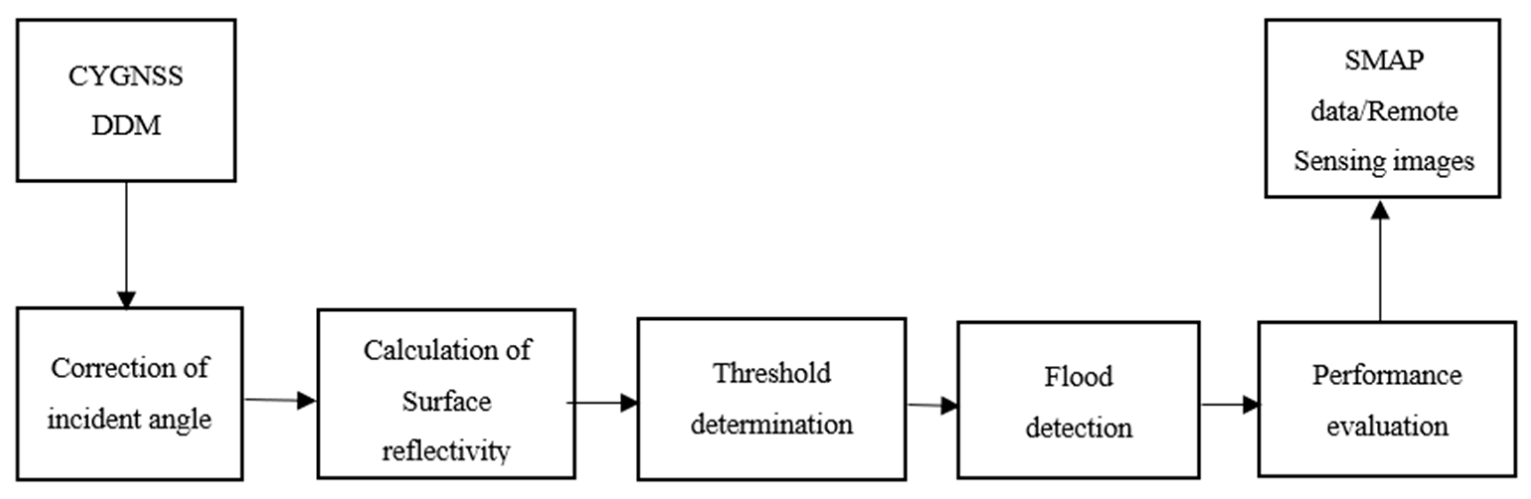
Zhang et al. used CYGNSS L1 data to detect and map flood inundation during the 2021 extreme precipitation in Henan Province, China [211]. Surface reflectivity (SR) derived by DDM data was used as the fundamental variable for mapping flood inundation. The SR threshold was determined by comparing the SR values of different land cover and land use in Henan Province. DDM data were also collected before and after the occurrence of floods in the same area. The effective isolated radiated power (EIRP), SR and SNR all increased when the studied area was submerged. The SMAP data was employed to validate the ability of submerged-area detection based on CYGNSS SR. The results show good agreement between the SMAP and CYGNSS SR. It is worth mentioning that CYGNSS SR has a higher resolution than SMAP, and it does not require information about the influences of uncertain factors such as cloud cover.
Yang et al. conducted a similar study, and employed the surface reflectivity from CYGNSS data to study daily flood monitoring in Henan, China [212]. The MODIS (Moderate Resolution Imaging Spectroradiometer) and SMAP data were used as the ground-truth data. The results indicated a strong correlation between high CYGNSS reflectivity and the flooded area monitored by MODIS. Both the brightness temperature and soil moisture from SMAP and CYGNSS reflectivity changed obviously in Zhengzhou and Xinxiang when the flood occurred. Figure 9 shows a simple flowchart of flood monitoring.
There are important characteristics of CYGNSS for dynamic flood monitoring, namely short revisit time and a higher resolution. In addition, if more GNSS-R satellites focusing on terrestrial applications are launched, the GNSS-R data will have better quality and higher spatial and temporal resolution and, thus, will further promote the land application of GNSS-R.
7.2. Tsunami Detection
A tsunami is a specific ocean wave that can be generated by an earthquake or a sudden sea floor displacement, underwater landslide or ocean volcano eruption. A tsunami may simply comprise a single solitary wave. The single wave can develop into a leading crest and a trailing wave train of gradually shorter and lower crests. Unlike wind-driven waves and swells, a tsunami can have a wavelength of a few hundred kilometers. Although a tsunami may measure a few decimeters in deep sea, it can be truly catastrophic; it can enormous damage and massive loss of life, as was the case with the 2004 Indian Ocean earthquake and the 2011 Tohoku earthquake in Japan [213,214]. This is mainly due to the fact that when the tsunami is close to the coast where the water depth is rather shallow, the stored energy gradually aggregates so that the wave height can be very high, such as several tens of meters.
To mitigate the impact of tsunamis, several tsunami warning centers have been established globally. These warning centers include the U.S. Pacific Tsunami Warning Centre [215] the Joint Australian Tsunami Warning Centre [216] and the German Indonesian Tsunami Early Warning System (GITEWS) [217]; these usually employ information inferred using data provided by the seismic station site network. Another way to enable tsunami warning is to use a network of pressure sensors deployed on the seafloor, to derive tsunami information using the modelled/empirical relationship between earthquake parameters and tsunami parameters [218].
A network of buoy-mounted sensors can also be used to monitor tsunamis in real-time to obtain the wave height, wavelength and wave propagation speed of a tsunami [219,220]. However, due to the deployment and maintenance cost, there is a limited number of buoyed sensors, which cover only a small part of the vast ocean surface. Satellite altimeters (e.g., Jason-1 radar altimeter) can provide relative sea level measurement with an accuracy of a few centimeters; thus, a Tsunami can be readily sensed if a satellite altimeter footprint goes through the wave [221], but the chance is rather small and there may be a significant delay in the observation due to the long revisit time.
GNSS-R possesses the potential for tsunami detection and parameter estimation, predicting the arrival of another technology for tsunami warnings. Helm et al. [222] and Stosius et al. [223] proposed the exploitation of space GNSS-R for tsunami detection, probably for the first time. Based on a tsunami model, preliminary results on tsunami detection through simulation were reported.
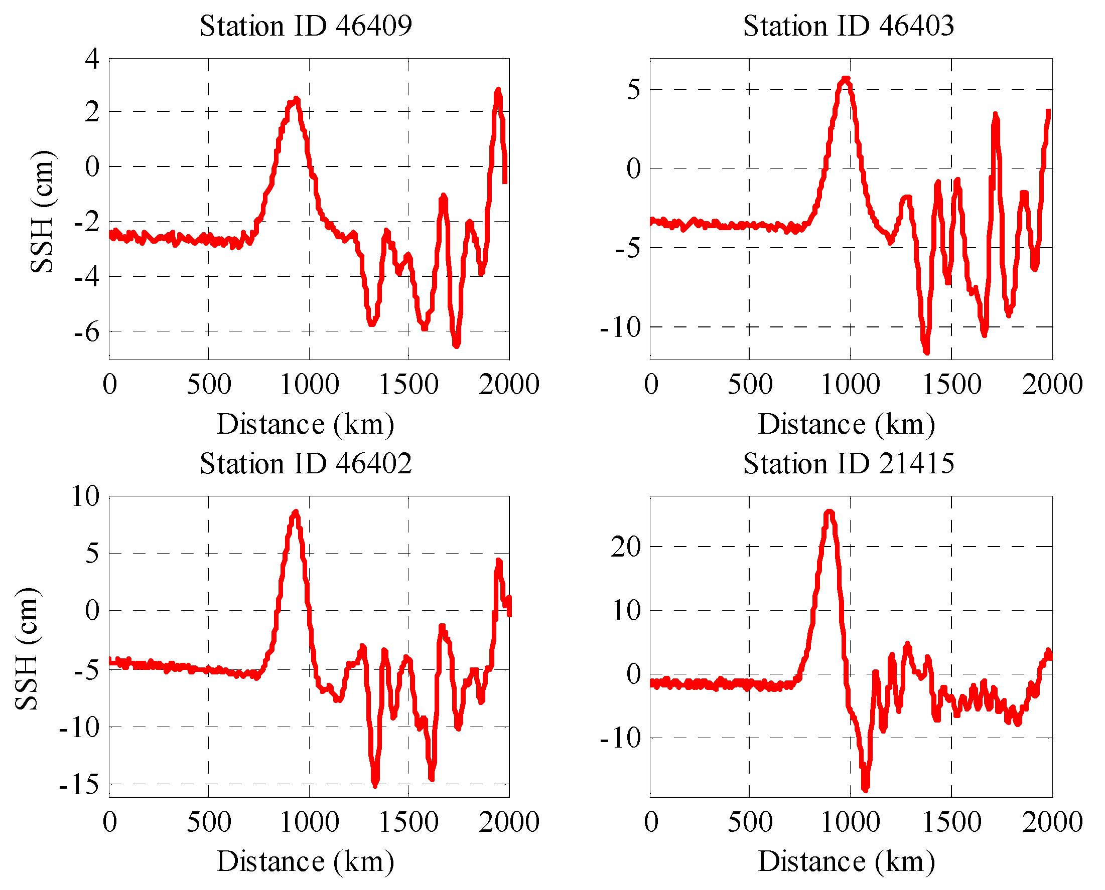
Tsunamis have different waveforms because they can be generated by different natural phenomena, as mentioned earlier. However, they often have similar patterns, especially the lead waves. Figure 10 shows the real SSH measurements, including four tsunami lead waves. The waveforms were generated by data measured by buoy-based sensors at observation stations when powerful tsunamis were triggered by the 2011 Tohoku earthquake in Japan [224]. Similar to radio and acoustic waves, the observed Tsunami wave amplitude is a function of time, and the Tsunami propagation speed can be more than 700 km/h. Note that considerable offset exists in the first three measured lead waves in Figure 10, probably due to the residual error in the removal of the solar and lunar tides.
Although the wavelength of a tsunami can be several hundred kilometers, the amplitude of a tsunami may also be around one meter, or even sub-decimeter, depending on the water depth and time delay. Tsunami waveforms may be simply modeled as triangles for convenience in theoretical analysis [225]. Due to the long wavelength and high propagation speed of tsunamis, it is impractical to detect tsunamis based on ground-based or airborne GNSS-R technology. Using spaceborne GNSS-R technology, it is possible to detect tsunamis, even during their early stage. Current GNSS-R related satellite missions mainly focus on ocean-surface wind speed measurement, such as for hurricanes and typhoons. Although the spaceborne data may also be utilized for sea surface altimetry, the accuracy might be rather low. In the case of strong measurement noise and a weak tsunami waveform, it is necessary to judge whether a tsunami is present by developing detection methods. A bin average (BA) may be considered as a simple method for tsunami detection [105]. Based on each BA output, a hypothesis test is applied to make a decision on whether a tsunami occurred. The selection of bin length is a significant issue. In terms of maximizing SNR, and assuming the tsunami lead wave is modelled as a simple isosceles triangle, the most suited bin length is determined as two thirds of the width of the tsunami lead wave, which does not include the remaining part of the tsunami with negative amplitude. To improve the detection probability, the sliding window moving average (SWMA) technique can be exploited, with the window being similar to a bin [226]. However, the difference is that the window moves one SSH measurement sample each time, and at a specific time point, the window will cover the main part of the waveform.
7.3. Estimation of Tsunami Parameters
It is also possible to measure the parameters of a Tsunami such as amplitude, width (or wavelength), propagation direction and speed [227]. This possibility mainly comes from the fact that a tsunami is a three-dimensional wave, and that multiple signal reflection tracks associated with multiple GNSS satellites may cross the wave. Suppose that a number of reflection tracks cross the wave and they are quite close to each other, so that the tsunami parameters can be roughly treated as the same over the intersection region. In fact, the parameters would be different over the region—mainly because water depth changes with location—so that the parameters such as tsunami amplitude and propagation velocity may change accordingly. However, each of the estimated parameters may be considered as the average of the parameter over the region.
As shown in Figure 11, the propagation direction can be defined as the azimuth angle, going clockwise from North, to the wave propagation direction (i.e., ). Point is the specific position on the cross section of the wave crossed by the ith reflection tract, and it may be chosen as the crest point of the wave. The reflection tracks are not displayed for clarity, and they do not play a useful role. Obtaining the accurate coordinates of the point is vital to obtaining an accurate estimation of the wave parameters. The positions may be determined after the reconstruction of the waveform, using methods such as wavelet transform [225]. As a well-developed theory [228,229], wavelet transform is effective for non-stationary signals that have short-lived transient components, such as tsunamis.
8. Conclusions and Future Research Directions
In this article, a comprehensive review is presented on spaceborne GNSS-R technology, which has achieved great advances in theory and practice; this is especially due to the recent successful launches of satellites related to GNSS-R, including the TDS-1 satellite in 2014, and the CYGNSS satellites in 2016. Current research progress and outcomes in spaceborne GNSS-R are described in six major sections. The focus of the review is on the detection of sea ice, tsunamis and sea surface rainfall, and on the retrieval of a range of geophysical parameters including sea-surface wind speed; significant wave height; sea surface rainfall intensity; sea surface height; sea ice thickness; tsunami lead wave height, propagation speed and directions; soil moisture; and vegetation.
In addition to the research topics on spaceborne GNSS-R studied in the preceding sections, there are other research topics in this exciting field that draw significant attention. For instance, Camps et al. studied ionospheric effects on spaceborne GNSS-R observations [230]. They utilized the global ionospheric scintillation model to analyze the total electron content and the scintillation index S4, and the results showed that scintillation mostly occurs from the transmitting space vehicle to ground. Note that ionospheric scintillation can degrade the signal-to-noise ratio and may cause coherent scattered components in low-wind regions. Thus, it is useful in enabling satellite data, such as from TechDemoSat-1 and CYGNSS missions, to infer ionospheric scintillation of spaceborne GNSS-R [231]. Wang and Morton employed the real GNSS-R data recorded by Spire Global Inc.’s LEMUR-2 CubeSats, to explore the potential of spaceborne GNSS-R measurements as a new data source for ionospheric TEC and plasma disturbance observation [232]. They employed geometry-free combinations of dual-frequency pseudorange and carrier-phase measurements to calculate ionospheric total electron content along a reflected path and direct path, respectively. Another example is the use of TDS-1 data to estimate the density of red tides, which mainly occur due to the continuous intensification of human activities in the ocean and have caused great harm to the marine environment and ecology. Ban et al. [233] proposed the use of spaceborne GNSS-R for red tide detection and its density estimation. They developed new models to associate GNSS-R observations with sea-surface red tide density. The Landsat-8 near-infrared data and TDS-1 GNSS-R data of a red tide outbreak in the sea off the Tsingtao coast in China were studied, and a model was built. The results of the model tests showed that the correlation coefficient was 0.73, and the RMSE of the retrieved the red tide density was 2.84%.
Although spaceborne GNSS-R has made great progress and many new concepts and methods have been proposed in recent years, as mentioned earlier, this technology is not yet mature. The developed empirical models and semi-empirical models are usually not generalized, so they may be only valid for rather limited scenarios. Therefore, it is desirable to enhance the models so that they can be widely applied. As an emerging remote sensing technology, it should be used to generate new products with performance comparable to the traditional remote sensing technologies, or combined with other technologies to obtain improved products. Another suggestion is to expand the applications of spaceborne GNSS-R to retrieve other geophysical parameters and detect other natural events or phenomena. Furthermore, it is always useful to build more advanced spaceborne GNSS-R sensors to improve their performance, such as sensitivity and SNR.
Author Contributions
All authors have made significant contributions to this manuscript. K.Y. designed the article structure, wrote Section 1, Section 7 and Section 8, and revised the paper; S.H. wrote Section 4 and Section 5 and organized the reference list; J.B. wrote Section 2 and Section 3; Y.A. wrote Section 5 and Section 6; Z.Z. wrote Section 4, Section 7 and Section 8; C.W. wrote Section 2; S.T. and J.W.C. made revisions. All authors have read and agreed to the published version of the manuscript.
Funding
This work was supported in part by the National Natural Science Foundation of China under Grants 42174022 and 41730109, and the Future Scientists Program of the China University of Mining and Technology under Grant 2020WLKXJ049.
Institutional Review Board Statement
Not applicable.
Informed Consent Statement
Not applicable.
Data Availability Statement
The data used in this paper are already given in the corresponding reference.
Acknowledgments
We are very grateful for the anonymous reviewers’ comments, which have greatly improved the quality and content of the manuscript.
Conflicts of Interest
The authors declare no conflict of interest.
References
- Larson, K.M.; Nievinski, F.G. GPS snow sensing: Results from the EarthScope Plate Boundary Observatory. Gps Solut. 2013, 17, 41–52. [Google Scholar] [CrossRef]
- Rodriguez-Alvarez, N.; Bosch-Lluis, X.; Camps, A.; Vall-llossera, M.; Valencia, E.; Fernando Marchan-Hernandez, J.; Ramos-Perez, I. Soil Moisture Retrieval Using GNSS-R Techniques: Experimental Results Over a Bare Soil Field. IEEE Trans. Geosci. Remote Sens. 2009, 47, 3616–3624. [Google Scholar] [CrossRef]
- Rodriguez-Alvarez, N.; Camps, A.; Vall-llossera, M.; Bosch-Lluis, X.; Monerris, A.; Ramos-Perez, I.; Valencia, E.; Fernando Marchan-Hernandez, J.; Martinez-Fernandez, J.; Baroncini-Turricchia, G.; et al. Land Geophysical Parameters Retrieval Using the Interference Pattern GNSS-R Technique. IEEE Trans. Geosci. Remote Sens. 2011, 49, 71–84. [Google Scholar] [CrossRef]
- Hall, C.D.; Cordey, R.A. Multistatic Scatterometry. In Proceedings of the International Geoscience and Remote Sensing Symposium, ‘Remote Sensing: Moving toward the 21st Century’, Edinburgh, UK, 12–16 September 1988; pp. 561–562. [Google Scholar]
- Martin-Neira, M. A Passive Reflectometry and Interferometry System (PARIS): Application to ocean altimetry. ESA J. 1993, 17, 331–355. [Google Scholar]
- Auber, J.C.; Bibaut, A.; Rigal, J.M. Characterization of multipath on land and sea at GPS frequencies. In Proceedings of the 7th International Technical Meeting of the Satellite Division of the Institute of Navigation, Salt Lake City, UT, USA, 20–23 September 1994; pp. 1155–1171. [Google Scholar]
- Katzberg, S.; Garrison, J. Utilizing GPS To Determine Ionospheric Delay over the Ocean; NASA Langley Technical Report Server: Washington, DC, USA, 1997.
- Garrison, J.L.; Katzberg, S.J.; Hill, M.I. Effect of sea roughness on bistatically scattered range coded signals from the Global Positioning System. Geophys. Res. Lett. 1998, 25, 2257–2260. [Google Scholar] [CrossRef] [Green Version]
- Kavak, A.; Vogel, W.J.; Xu, G. Using GPS to measure ground complex permittivity. Electron. Lett. 1998, 34, 254–255. [Google Scholar] [CrossRef]
- Komjathy, A.; Zavorotny, V.; Axelrad, P.; Born, G.; Garrison, J. Gps Signal Scattering from Sea Surface: Comparison between Experimental Data and Theoretical Model. In Proceedings of the Fifth International Conference on Remote Sensing for Marine and Coastal Environments, San Diego, CA, USA, 5–7 October 1998. [Google Scholar]
- Anderson, K.D. Determination of water level and tides using interferometric observations of GPS signals. J. Atmos. Ocean. Technol. 2000, 17, 1118–1127. [Google Scholar] [CrossRef]
- Masters, D.; Zavorotny, V.; Katzberg, S.; Emery, W. GPS signal scattering from land for moisture content determination. In Proceedings of the IGARSS 2000, IEEE 2000 International Geoscience and Remote Sensing Symposium. Taking the Pulse of the Planet: The Role of Remote Sensing in Managing the Environment. Proceedings (Cat. No.00CH37120), Honolulu, HI, USA, 24–28 July 2000; Volume 3097, pp. 3090–3092. [Google Scholar]
- Zavorotny, V.U.; Voronovich, A.G. Bistatic GPS signal reflections at various polarizations from rough land surface with moisture content. In Proceedings of the IGARSS 2000, IEEE 2000 International Geoscience and Remote Sensing Symposium. Taking the Pulse of the Planet: The Role of Remote Sensing in Managing the Environment. Proceedings (Cat. No.00CH37120), Honolulu, HI, USA, 24–28 July 2000; Volume 2857, pp. 2852–2854. [Google Scholar]
- Komjathy, A.; Garrison, J.L.; Zavorotny, V. GPS: A new tool for ocean science. GPS World 1999, 10, 50–56. [Google Scholar]
- Zavorotny, V.U.; Voronovich, A.G. Scattering of GPS signals from the ocean with wind remote sensing application. IEEE Trans. Geosci. Remote Sens. 2000, 38, 951–964. [Google Scholar] [CrossRef] [Green Version]
- Katzberg, S.J.; Walker, R.A.; Roles, J.H.; Lynch, T.; Black, P.G. First GPS signals reflected from the interior of a tropical storm: Preliminary results from Hurricane Michael. Geophys. Res. Lett. 2001, 28, 1981–1984. [Google Scholar] [CrossRef] [Green Version]
- Treuhaft, R.N.; Lowe, S.T.; Zuffada, C.; Chao, Y. 2-cm GPS altimetry over Crater Lake. Geophys. Res. Lett. 2001, 28, 4343–4346. [Google Scholar] [CrossRef]
- Gleason, S.; Gebre-Egziabher, D.; Egziabher, D.G. GNSS Applications and Methods; Artech House: London, UK, 2009. [Google Scholar]
- Jin, S.; Cardellach, E.; Xie, F. GNSS Remote Sensing: Theory, Methods and Applications. Remote Sens. Digit. Image Process. 2013, 19. [Google Scholar] [CrossRef]
- Jin, S.; Feng, G.P.; Gleason, S. Remote sensing using GNSS signals: Current status and future directions. Adv. Space Res. 2011, 47, 1645–1653. [Google Scholar] [CrossRef]
- Yu, K. Theory and Practice of GNSS Reflectometry; Springer Nature: Berlin/Heidelberg, Germany, 2021. [Google Scholar]
- Yu, K.; Rizos, C.; Burrage, D.; Dempster, A.G.; Zhang, K.; Markgraf, M. An overview of GNSS remote sensing. Eurasip J. Adv. Signal Process. 2014, 1, 134. [Google Scholar] [CrossRef] [Green Version]
- Zavorotny, V.U.; Gleason, S.; Cardellach, E.; Camps, A. Tutorial on Remote Sensing Using GNSS Bistatic Radar of Opportunity. IEEE Geosci. Remote Sens. Mag. 2014, 2, 8–45. [Google Scholar] [CrossRef] [Green Version]
- Clarizia, M.P.; Gommenginger, C.; Gleason, S.; Galdi, C.; Unwin, M. Global Navigation Satellite System-Reflectometry (GNSS-R) from the UK-DMC Satellite for Remote Sensing of the Ocean Surface. In Proceedings of the IGARSS 2008—2008 IEEE International Geoscience and Remote Sensing Symposium, Boston, MA, USA, 8–11 July 2008; pp. I-276–I-279. [Google Scholar]
- Tye, J.; Jales, P.; Unwin, M.; Underwood, C. The First Application of Stare Processing to Retrieve Mean Square Slope Using the SGR-ReSI GNSS-R Experiment on TDS-1. IEEE J. Sel. Top. Appl. Earth Obs. Remote Sens. 2016, 9, 4669–4677. [Google Scholar] [CrossRef]
- Unwin, M.; Jales, P.; Tye, J.; Gommenginger, C.; Foti, G.; Rosello, J. Spaceborne GNSS-Reflectometry on TechDemoSat-1: Early Mission Operations and Exploitation. IEEE J. Sel. Top. Appl. Earth Obs. Remote Sens. 2016, 9, 4525–4539. [Google Scholar] [CrossRef]
- Clarizia, M.P.; Ruf, C.S. Wind Speed Retrieval Algorithm for the Cyclone Global Navigation Satellite System (CYGNSS) Mission. IEEE Trans. Geosci. Remote Sens. 2016, 54, 4419–4432. [Google Scholar] [CrossRef]
- Ruf, C.; Lyons, A.; Unwin, M.; Dickinson, J.; Rose, R.; Rose, D.; Vincent, M. CYGNSS: Enabling the Future of Hurricane Prediction. IEEE Geosci. Remote Sens. Mag. 2013, 1, 52–67. [Google Scholar] [CrossRef]
- Weathernews WNISAT-1R. Available online: https://global.weathernews.com/infrastructure/wnisat-1/ (accessed on 15 December 2021).
- Jing, C.; Niu, X.; Duan, C.; Lu, F.; Di, G.; Yang, X. Sea Surface Wind Speed Retrieval from the First Chinese GNSS-R Mission: Technique and Preliminary Results. Remote Sens. 2019, 11, 3013. [Google Scholar] [CrossRef] [Green Version]
- Xinliang, N.; Feng, L.; Yuanhua, L.; Cheng, J.; Wan, B. Application and Technology of Bufeng-1 GNSSR Demonstration Satellites on Sea Surface Wind Speed Detection; China Satellite Navigation Office Academic Exchange Center: Chengdu, China, 2020; p. 21.
- GPSWorld SSTL Demonstrates New GNSS-R Capabilities. Available online: https://www.gpsworld.com/sstl-demonstrates-new-gnss-r-capabilities/ (accessed on 15 November 2021).
- Zhang, P.; Hu, X.; Lu, Q.; Zhu, A.; Lin, M.; Sun, L.; Chen, L.; Xu, N. FY-3E: The First Operational Meteorological Satellite Mission in an Early Morning Orbit. Adv. Atmos. Sci. 2021, 39, 1–8. [Google Scholar] [CrossRef]
- Clarizia, M.P.; Gommenginger, C.P.; Gleason, S.T.; Srokosz, M.A.; Galdi, C.; Di Bisceglie, M. Analysis of GNSS-R delay-Doppler maps from the UK-DMC satellite over the ocean. Geophys. Res. Lett. 2009, 36. [Google Scholar] [CrossRef] [Green Version]
- Malik, J.S.; Bhatti, U.I. Remote Sensing of Ocean, Ice and Land Surfaces Using Bistatically Reflected GNSS Signals From Low Earth Orbit. In Proceedings of the 4th International Conference on Aerospace Science and Engineering (ICASE), Islamabad, Pakistan, 2–4 September 2015. [Google Scholar]
- Clarizia, M.P.; Ruf, C.S.; Jales, P.; Gommenginger, C. Spaceborne GNSS-R Minimum Variance Wind Speed Estimator. IEEE Trans. Geosci. Remote Sens. 2014, 52, 6829–6843. [Google Scholar] [CrossRef]
- Li, C.; Huang, W. An Algorithm for Sea-Surface Wind Field Retrieval From GNSS-R Delay-Doppler Map. IEEE Geosci. Remote Sens. Lett. 2014, 11, 2110–2114. [Google Scholar] [CrossRef]
- Foti, G.; Gommenginger, C.; Jales, P.; Unwin, M.; Shaw, A.; Robertson, C.; Rosello, J. Spaceborne GNSS reflectometry for ocean winds: First results from the UK TechDemoSat-1 mission. Geophys. Res. Lett. 2015, 42, 5435–5441. [Google Scholar] [CrossRef] [Green Version]
- Soisuvarn, S.; Jelenak, Z.; Said, F.; Chang, P.S.; Egido, A. The GNSS Reflectometry Response to the Ocean Surface Winds and Waves. IEEE J. Sel. Top. Appl. Earth Obs. Remote Sens. 2016, 9, 4678–4699. [Google Scholar] [CrossRef]
- Rodriguez-Alvarez, N.; Garrison, J.L. Generalized Linear Observables for Ocean Wind Retrieval From Calibrated GNSS-R Delay-Doppler Maps. IEEE Trans. Geosci. Remote Sens. 2016, 54, 1142–1155. [Google Scholar] [CrossRef]
- Wang, F.; Yang, D.; Zhang, B.; Li, W. Waveform-based spaceborne GNSS-R wind speed observation: Demonstration and analysis using UK TechDemoSat-1 data. Adv. Space Res. 2018, 61, 1573–1587. [Google Scholar] [CrossRef]
- Ruf, C.S.; Balasubramaniam, R. Development of the CYGNSS Geophysical Model Function for Wind Speed. IEEE J. Sel. Top. Appl. Earth Obs. Remote Sens. 2019, 12, 66–77. [Google Scholar] [CrossRef]
- Ruf, C.S.; Gleason, S.; McKague, D.S. Assessment of CYGNSS Wind Speed Retrieval Uncertainty. IEEE J. Sel. Top. Appl. Earth Obs. Remote Sens. 2019, 12, 87–97. [Google Scholar] [CrossRef]
- Dong, Z.; Jin, S. Evaluation of Spaceborne GNSS-R Retrieved Ocean Surface Wind Speed with Multiple Datasets. Remote Sens. 2019, 11, 2747. [Google Scholar] [CrossRef] [Green Version]
- Liu, Y.; Collett, I.; Morton, Y.J. Application of Neural Network to GNSS-R Wind Speed Retrieval. IEEE Trans. Geosci. Remote Sens. 2019, 57, 9756–9766. [Google Scholar] [CrossRef]
- Asgarimehr, M.; Zhelavskaya, I.; Foti, G.; Reich, S.; Wickert, J. A GNSS-R Geophysical Model Function: Machine Learning for Wind Speed Retrievals. IEEE Geosci. Remote Sens. Lett. 2020, 17, 1333–1337. [Google Scholar] [CrossRef]
- Balasubramaniam, R.; Ruf, C. Neural Network Based Quality Control of CYGNSS Wind Retrieval. Remote Sens. 2020, 12, 2859. [Google Scholar] [CrossRef]
- Kasantikul, K.; Yang, D.; Wang, Q.; Lwin, A. A Novel Wind Speed Estimation Based on the Integration of an Artificial Neural Network and a Particle Filter Using BeiDou GEO Reflectometry. Sensors 2018, 18, 3350. [Google Scholar] [CrossRef] [PubMed] [Green Version]
- Reynolds, J.; Clarizia, M.P.; Santi, E. Wind Speed Estimation From CYGNSS Using Artificial Neural Networks. IEEE J. Sel. Top. Appl. Earth Obs. Remote Sens. 2020, 13, 708–716. [Google Scholar] [CrossRef]
- Chu, X.; He, J.; Song, H.; Qi, Y.; Sun, Y.; Bai, W.; Li, W.; Wu, Q. Multimodal Deep Learning for Heterogeneous GNSS-R Data Fusion and Ocean Wind Speed Retrieval. IEEE J. Sel. Top. Appl. Earth Obs. Remote Sens. 2020, 13, 5971–5981. [Google Scholar] [CrossRef]
- Guo, W.; Du, H.; Cheong, J.W.; Southwell, B.J.; Dempster, A.G. GNSS-R Wind Speed Retrieval of Sea Surface Based on Particle Swarm Optimization Algorithm. IEEE Trans. Geosci. Remote Sens. 2021, 60, 1–14. [Google Scholar] [CrossRef]
- Hammond, M.L.; Foti, G.; Rawlinson, J.; Gommenginger, C.; Srokosz, M.; King, L.; Unwin, M.; Rosello, J. First Assessment of Geophysical Sensitivities from Spaceborne Galileo and BeiDou GNSS-Reflectometry Data Collected by the UK TechDemoSat-1 Mission. Remote Sens. 2020, 12, 2927. [Google Scholar] [CrossRef]
- Wang, H.-Y.; Juang, J.-C. Retrieval of Ocean Surface Wind Speed Using Reflected BPSK/BOC Signals. Remote Sens. 2020, 12, 2698. [Google Scholar] [CrossRef]
- Said, F.; Jelenak, Z.; Park, J.; Chang, P.S. The NOAA Track-Wise Wind Retrieval Algorithm and Product Assessment for CyGNSS. IEEE Trans. Geosci. Remote Sens. 2021, 60, 1–24. [Google Scholar] [CrossRef]
- Said, F.; Jelenak, Z.; Chang, P.S.; Soisuvarn, S. An Assessment of CYGNSS Normalized Bistatic Radar Cross Section Calibration. IEEE J. Sel. Top. Appl. Earth Obs. Remote Sens. 2019, 12, 50–65. [Google Scholar] [CrossRef]
- Gleason, S. Space-Based GNSS Scatterometry: Ocean Wind Sensing Using an Empirically Calibrated Model. IEEE Trans. Geosci. Remote Sens. 2013, 51, 4853–4863. [Google Scholar] [CrossRef]
- Gleason, S.; Ruf, C.S.; Clarizia, M.P.; O’Brien, A.J. Calibration and Unwrapping of the Normalized Scattering Cross Section for the Cyclone Global Navigation Satellite System. IEEE Trans. Geosci. Remote Sens. 2016, 54, 2495–2509. [Google Scholar] [CrossRef]
- Jing, C.; Yang, X.; Ma, W.; Yu, Y.; Dong, D.; Li, Z.; Xu, C. Retrieval of sea surface winds under hurricane conditions from GNSS-R observations. Acta Oceanol. Sin. 2016, 35, 91–97. [Google Scholar] [CrossRef]
- Bu, J.; Yu, K.; Zhu, Y.; Qian, N.; Chang, J. Developing and Testing Models for Sea Surface Wind Speed Estimation with GNSS-R Delay Doppler Maps and Delay Waveforms. Remote Sens. 2020, 12, 3760. [Google Scholar] [CrossRef]
- Pascual, D.; Clarizia, M.P.; Ruf, C.S. Improved CYGNSS Wind Speed Retrieval Using Significant Wave Height Correction. Remote Sens. 2021, 13, 4313. [Google Scholar] [CrossRef]
- Li, X.H.; Yang, D.K.; Yang, J.S.; Zheng, G.; Han, G.Q.; Nan, Y.; Li, W.Q. Analysis of coastal wind speed retrieval from CYGNSS mission using artificial neural network. Remote Sens. Environ. 2021, 260, 112454. [Google Scholar] [CrossRef]
- Asgarimehr, M.; Arnold, C.; Weigel, T.; Ruf, C.; Wickert, J. GNSS reflectometry global ocean wind speed using deep learning: Development and assessment of CyGNSSnet. Remote Sens. Environ. 2022, 269, 112801. [Google Scholar] [CrossRef]
- Guo, W.; Du, H.; Guo, C.; Southwell, B.J.; Cheong, J.W.; Dempster, A.G. Information fusion for GNSS-R wind speed retrieval using statistically modified convolutional neural network. Remote Sens. Environ. 2022, 272, 112934. [Google Scholar] [CrossRef]
- Zheng, C.W.; Li, C.Y. Variation of the wave energy and significant wave height in the China Sea and adjacent waters. Renew. Sustain. Energy Rev. 2015, 43, 381–387. [Google Scholar] [CrossRef]
- Holthuijsen, L. Waves in Oceanic and Coastal Waters; Cambridge University Press: Cambridge, UK, 2007; p. 404. [Google Scholar] [CrossRef]
- Yang, J.; Zhang, J.; Jia, Y.; Fan, C.; Cui, W. Validation of Sentinel-3A/3B and Jason-3 Altimeter Wind Speeds and Significant Wave Heights Using Buoy and ASCAT Data. Remote Sens. 2020, 12, 2079. [Google Scholar] [CrossRef]
- Xue, S.; Geng, X.; Yan, X.-H.; Xie, T.; Yu, Q. Significant wave height retrieval from Sentinel-1 SAR imagery by convolutional neural network. J. Oceanogr. 2020, 76, 465–477. [Google Scholar] [CrossRef]
- Wang, B.; Li, M.; Liu, S.; Chen, S.; Zhu, Q.; Wang, H. Current status and trend of ocean data buoy observation technology applications. Chin. J. Sci. Instrum. 2014, 35, 2401–2414. [Google Scholar] [CrossRef]
- Peng, Q.; Jin, S. Significant Wave Height Estimation from Space-Borne Cyclone-GNSS Reflectometry. Remote Sens. 2019, 11, 584. [Google Scholar] [CrossRef] [Green Version]
- Alpers, W.; Hasselmann, K. Spectral signal to clutter and thermal noise properties of ocean wave imaging synthetic aperture radars. Int. J. Remote Sens. 1982, 3, 423–446. [Google Scholar] [CrossRef]
- Yang, S.; Jin, S.; Jia, Y.; Ye, M. Significant Wave Height Estimation from Joint CYGNSS DDMA and LES Observations. Sensors 2021, 21, 6123. [Google Scholar] [CrossRef] [PubMed]
- Bu, J.; Yu, K. Significant Wave Height Retrieval Method Based on Spaceborne GNSS Reflectometry. IEEE Geosci. Remote Sens. Lett. 2022, 19, 1–5. [Google Scholar] [CrossRef]
- Liu, X.; Huang, W.; Gill, E.W. Wind Direction Estimation From Rain-Contaminated Marine Radar Data Using the Ensemble Empirical Mode Decomposition Method. IEEE Trans. Geosci. Remote Sens. 2017, 55, 1833–1841. [Google Scholar] [CrossRef]
- Lund, B.; Graber, H.C.; Romeiser, R. Wind Retrieval From Shipborne Nautical X-Band Radar Data. IEEE Trans. Geosci. Remote Sens. 2012, 50, 3800–3811. [Google Scholar] [CrossRef]
- Chen, X.; Huang, W.; Zhao, C.; Tian, Y. Rain Detection From X-Band Marine Radar Images: A Support Vector Machine-Based Approach. IEEE Trans. Geosci. Remote Sens. 2020, 58, 2115–2123. [Google Scholar] [CrossRef]
- Zheng, Y.; Shi, Z.; Lu, Z.; Ma, W. A Method for Detecting Rainfall From X-Band Marine Radar Images. IEEE Access 2020, 8, 19046–19057. [Google Scholar] [CrossRef]
- Lu, Z.; Sun, L.; Zhou, Y. A Method for Rainfall Detection and Rainfall Intensity Level Retrieval from X-Band Marine Radar Images. Appl. Sci. 2021, 11, 1565. [Google Scholar] [CrossRef]
- Xue, M.; Hang, R.; Liu, Q.; Yuan, X.-T.; Lu, X. CNN-based near-real-time precipitation estimation from Fengyun-2 satellite over Xinjiang, China. Atmos. Res. 2021, 250, 105337. [Google Scholar] [CrossRef]
- Ma, Q.; Li, Y.; Feng, H.; Yu, Q.; Zou, Y.; Liu, F.; Pulatov, B. Performance evaluation and correction of precipitation data using the 20-year IMERG and TMPA precipitation products in diverse subregions of China. Atmos. Res. 2021, 249, 105304. [Google Scholar] [CrossRef]
- Tang, G.; Clark, M.P.; Papalexiou, S.M.; Ma, Z.; Hong, Y. Have satellite precipitation products improved over last two decades? A comprehensive comparison of GPM IMERG with nine satellite and reanalysis datasets. Remote Sens. Environ. 2020, 240, 111697. [Google Scholar] [CrossRef]
- Yu, C.; Hu, D.; Liu, M.; Wang, S.; Di, Y. Spatio-temporal accuracy evaluation of three high-resolution satellite precipitation products in China area. Atmos. Res. 2020, 241, 104952. [Google Scholar] [CrossRef]
- Peng, F.; Zhao, S.; Chen, C.; Cong, D.; Wang, Y.; Ouyang, H. Evaluation and comparison of the precipitation detection ability of multiple satellite products in a typical agriculture area of China. Atmos. Res. 2020, 236, 104814. [Google Scholar] [CrossRef]
- Huang, W.-R.; Liu, P.-Y.; Chang, Y.-H.; Liu, C.-Y. Evaluation and Application of Satellite Precipitation Products in Studying the Summer Precipitation Variations over Taiwan. Remote Sens. 2020, 12, 347. [Google Scholar] [CrossRef] [Green Version]
- Yang, M.; Liu, G.; Chen, T.; Chen, Y.; Xia, C. Evaluation of GPM IMERG precipitation products with the point rain gauge records over Sichuan, China. Atmos. Res. 2020, 246, 105101. [Google Scholar] [CrossRef]
- Keikhosravi Kiany, M.S.; Masoodian, S.A.; Balling Jr, R.C.; Montazeri, M. Evaluation of the TRMM 3B42 product for extreme precipitation analysis over southwestern Iran. Adv. Space Res. 2020, 66, 2094–2112. [Google Scholar] [CrossRef]
- Zhang, C.; Wang, H.; Zeng, J.; Ma, L.; Guan, L. Short-Term Dynamic Radar Quantitative Precipitation Estimation Based on Wavelet Transform and Support Vector Machine. J. Meteorol. Res. 2020, 34, 413–426. [Google Scholar] [CrossRef]
- Chen, Z.; He, Y.; Zhang, B. An Automatic Algorithm to Retrieve Wave Height From X-Band Marine Radar Image Sequence. IEEE Trans. Geosci. Remote Sens. 2017, 55, 5084–5092. [Google Scholar] [CrossRef]
- Tian, W.; Yi, L.; Liu, W.; Huang, W.; Ma, G.; Zhang, Y. Ground radar precipitation estimation with deep learning approaches in meteorological private cloud. J. Cloud Comput. 2020, 9, 22. [Google Scholar] [CrossRef] [Green Version]
- Chen, H.; Yong, B.; Shen, Y.; Liu, J.; Hong, Y.; Zhang, J. Comparison analysis of six purely satellite-derived global precipitation estimates. J. Hydrol. 2020, 581, 124376. [Google Scholar] [CrossRef]
- Islam, M.A.; Yu, B.; Cartwright, N. Assessment and comparison of five satellite precipitation products in Australia. J. Hydrol. 2020, 590, 125474. [Google Scholar] [CrossRef]
- Ayoub, A.B.; Tangang, F.; Juneng, L.; Tan, M.L.; Chung, J.X. Evaluation of Gridded Precipitation Datasets in Malaysia. Remote Sens. 2020, 12, 613. [Google Scholar] [CrossRef] [Green Version]
- Hussain, Y.; Satgé, F.; Hussain, M.B.; Martinez-Carvajal, H.; Bonnet, M.-P.; Cárdenas-Soto, M.; Roig, H.L.; Akhter, G. Performance of CMORPH, TMPA, and PERSIANN rainfall datasets over plain, mountainous, and glacial regions of Pakistan. Theor. Appl. Climatol. 2017, 131, 1119–1132. [Google Scholar] [CrossRef]
- Hamza, A.; Anjum, M.N.; Masud Cheema, M.J.; Chen, X.; Afzal, A.; Azam, M.; Kamran Shafi, M.; Gulakhmadov, A. Assessment of IMERG-V06, TRMM-3B42V7, SM2RAIN-ASCAT, and PERSIANN-CDR Precipitation Products over the Hindu Kush Mountains of Pakistan, South Asia. Remote Sens. 2020, 12, 3871. [Google Scholar] [CrossRef]
- Zhang, Y.; Hanati, G.; Danierhan, S.; Liu, Q.; Xu, Z. Evaluation and Comparison of Daily GPM/TRMM Precipitation Products over the Tianshan Mountains in China. Water 2020, 12, 3088. [Google Scholar] [CrossRef]
- Carreno-Luengo, H.; Camps, A.; Ruf, C.; Floury, N.; Martin-Neira, M.; Wang, T.; Khalsa, S.J.; Clarizia, M.P.; Reynolds, J.; Johnson, J.; et al. The IEEE-SA Working Group on Spaceborne GNSS-R: Scene Study. IEEE Access 2021, 9, 89906–89933. [Google Scholar] [CrossRef]
- Llaveria, D.; Munoz-Martin, J.F.; Herbert, C.; Pablos, M.; Park, H.; Camps, A. Sea Ice Concentration and Sea Ice Extent Mapping with L-Band Microwave Radiometry and GNSS-R Data from the FFSCat Mission Using Neural Networks. Remote Sens. 2021, 13, 1139. [Google Scholar] [CrossRef]
- Munoz-Martin, J.F.; Fernandez, L.; Perez, A.; Ruiz-de-Azua, J.A.; Park, H.; Camps, A.; Domínguez, B.C.; Pastena, M. In-Orbit Validation of the FMPL-2 Instrument—The GNSS-R and L-Band Microwave Radiometer Payload of the FSSCat Mission. Remote Sens. 2020, 13, 121. [Google Scholar] [CrossRef]
- Juang, J.; Tsai, Y.; Lin, C. FORMOSAT-7R Mission for GNSS Reflectometry. In Proceedings of the IGARSS 2019—2019 IEEE International Geoscience and Remote Sensing Symposium, Yokohama, Japan, 28 July–2 August 2019; pp. 5177–5180. [Google Scholar]
- Juang, J.C.; Lin, C.T.; Tsai, Y.F. Comparison and Synergy of BPSK and BOC Modulations in GNSS Reflectometry. IEEE J. Sel. Top. Appl. Earth Observ. Remote Sens. 2020, 13, 1959–1971. [Google Scholar] [CrossRef]
- Juang, J.C.; Ma, S.H.; Lin, C.T. Study of GNSS-R Techniques for FORMOSAT Mission. IEEE J. Sel. Top. Appl. Earth Observ. Remote Sens. 2016, 9, 4582–4592. [Google Scholar] [CrossRef]
- Hammond, M.L.; Foti, G.; Gommenginger, C.; Srokosz, M. Temporal variability of GNSS-Reflectometry ocean wind speed retrieval performance during the UK TechDemoSat-1 mission. Remote Sens. Environ. 2020, 242, 111744. [Google Scholar] [CrossRef]
- Li, W.; Rius, A.; Fabra, F.; Cardellach, E.; Ribo, S.; Martin-Neira, M. Revisiting the GNSS-R Waveform Statistics and Its Impact on Altimetric Retrievals. IEEE Trans. Geosci. Remote Sens. 2018, 56, 2854–2871. [Google Scholar] [CrossRef]
- Yu, K.; Li, Y.; Chang, X. Snow Depth Estimation Based on Combination of Pseudorange and Carrier Phase of GNSS Dual-Frequency Signals. IEEE Trans. Geosci. Remote Sens. 2019, 57, 1817–1828. [Google Scholar] [CrossRef]
- Yan, Q.; Huang, W.; Moloney, C. Neural Networks Based Sea Ice Detection and Concentration Retrieval From GNSS-R Delay-Doppler Maps. IEEE J. Sel. Top. Appl. Earth Obs. Remote Sens. 2017, 10, 3789–3798. [Google Scholar] [CrossRef]
- Yu, K. Weak Tsunami Detection Using GNSS-R-Based Sea Surface Height Measurement. IEEE Trans. Geosci. Remote Sens. 2016, 54, 1363–1375. [Google Scholar] [CrossRef]
- Camps, A.; Park, H.; Castellvi, J.; Corbera, J.; Ascaso, E. Single-Pass Soil Moisture Retrievals Using GNSS-R: Lessons Learned. Remote Sens. 2020, 12, 2064. [Google Scholar] [CrossRef]
- Cardellach, E.; Nan, Y.; Li, W.; Padullés, R.; Ribó, S.; Rius, A. Variational Retrievals of High Winds Using Uncalibrated CyGNSS Observables. Remote Sens. 2020, 12, 3930. [Google Scholar] [CrossRef]
- Asgarimehr, M.; Zavorotny, V.; Wickert, J.; Reich, S. Can GNSS Reflectometry Detect Precipitation Over Oceans? Geophys. Res. Lett. 2018, 45, 12585–12592. [Google Scholar] [CrossRef] [Green Version]
- Asgarimehr, M.; Hoseini, M.; Semmling, M.; Ramatschi, M.; Camps, A.; Nahavandchi, H.; Haas, R.; Wickert, J. Remote Sensing of Precipitation Using Reflected GNSS Signals: Response Analysis of Polarimetric Observations. IEEE Trans. Geosci. Remote Sens. 2021, 60, 1–12. [Google Scholar] [CrossRef]
- Asgarimehr, M.; Wickert, J.; Reich, S. Evaluating Impact of Rain Attenuation on Space-borne GNSS Reflectometry Wind Speeds. Remote Sens. 2019, 11, 1048. [Google Scholar] [CrossRef] [Green Version]
- Balasubramaniam, R.; Ruf, C. Characterization of rain impact on L-Band GNSS-R ocean surface measurements. Remote Sens. Environ. 2020, 239, 111607. [Google Scholar] [CrossRef]
- Bu, J.; Yu, K. Sea Surface Rainfall Detection and Intensity Retrieval Based on GNSS-Reflectometry Data from the CYGNSS Mission. IEEE Trans. Geosci. Remote Sens. 2021, 60, 1–15. [Google Scholar] [CrossRef]
- Clarizia, M.P.; Ruf, C.; Cipollini, P.; Zuffada, C. First spaceborne observation of sea surface height using GPS-Reflectometry. Geophys. Res. Lett. 2016, 43, 767–774. [Google Scholar] [CrossRef] [Green Version]
- Li, W.; Cardellach, E.; Fabra, F.; Rius, A.; Ribo, S.; Martin-Neira, M. First spaceborne phase altimetry over sea ice using TechDemoSat-1 GNSS-R signals. Geophys. Res. Lett. 2017, 44, 8369–8376. [Google Scholar] [CrossRef]
- Mashburn, J.; Axelrad, P.; Lowe, S.T.; Larson, K.M. Global Ocean Altimetry with GNSS Reflections from TechDemoSat-1. IEEE Trans. Geosci. Remote Sens. 2018, 56, 4088–4097. [Google Scholar] [CrossRef]
- Hu, C.; Benson, C.R.; Rizos, C.; Qiao, L. Impact of Receiver Dynamics on Space-Based GNSS-R Altimetry. IEEE J. Sel. Top. Appl. Earth Obs. Remote Sens. 2019, 12, 1974–1980. [Google Scholar] [CrossRef]
- Xu, L.; Wan, W.; Chen, X.; Zhu, S.; Liu, B.; Hong, Y. Spaceborne GNSS-R Observation of Global Lake Level: First Results from the TechDemoSat-1 Mission. Remote Sens. 2019, 11, 1438. [Google Scholar] [CrossRef] [Green Version]
- Li, W.; Cardellach, E.; Fabra, F.; Ribo, S.; Rius, A. Assessment of Spaceborne GNSS-R Ocean Altimetry Performance Using CYGNSS Mission Raw Data. IEEE Trans. Geosci. Remote Sens. 2020, 58, 238–250. [Google Scholar] [CrossRef]
- Qiu, H.; Jin, S. Global Mean Sea Surface Height Estimated from Spaceborne Cyclone-GNSS Reflectometry. Remote Sens. 2020, 12, 356. [Google Scholar] [CrossRef] [Green Version]
- Mashburn, J.; Axelrad, P.; Zuffada, C.; Loria, E.; O’Brien, A.; Haines, B. Improved GNSS-R Ocean Surface Altimetry with CYGNSS in the Seas of Indonesia. IEEE Trans. Geosci. Remote Sens. 2020, 58, 6071–6087. [Google Scholar] [CrossRef]
- Hu, C.; Benson, C.R.; Qiao, L.; Rizos, C. The Validation of the Weight Function in the Leading-Edge-Derivative Path Delay Estimator for Space-Based GNSS-R Altimetry. IEEE Trans. Geosci. Remote Sens. 2020, 58, 6243–6254. [Google Scholar] [CrossRef]
- Song, M.; He, X.; Wang, X.; Jia, D.; Xiao, R.; Shi, H.; Wu, Y. Study on the Exploration of Spaceborne GNSS-R Raw Data Focusing on Altimetry. IEEE J. Sel. Top. Appl. Earth Obs. Remote Sens. 2020, 13, 6142–6154. [Google Scholar] [CrossRef]
- Zhang, Q.; Liu, Y.; Xia, J. Space-Borne GNSS-R Ionospheric Delay Error Elimination by Optimal Spatial Filtering. Sensors 2020, 20, 5535. [Google Scholar] [CrossRef]
- Cardellach, E.; Li, W.; Rius, A.; Semmling, M.; Wickert, J.; Zus, F.; Ruf, C.; Buontempo, C. First Precise Spaceborne Sea Surface Altimetry with GNSS Reflected Signals. IEEE J. Sel. Top. Appl. Earth Obs. Remote Sens. 2020, 13, 102–112. [Google Scholar] [CrossRef]
- Wang, Y.; Breitsch, B.; Morton, Y.T.J. A State-Based Method to Simultaneously Reduce Cycle Slips and Noise in Coherent GNSS-R Phase Measurements From Open-Loop Tracking. IEEE Trans. Geosci. Remote Sens. 2021, 59, 8873–8884. [Google Scholar] [CrossRef]
- Cui, Z.; Zheng, W.; Wu, F.; Li, X.; Zhu, C.; Liu, Z.; Ma, X. Improving GNSS-R Sea Surface Altimetry Precision Based on the Novel Dual Circularly Polarized Phased Array Antenna Model. Remote Sens. 2021, 13, 2974. [Google Scholar] [CrossRef]
- Carreno-Luengo, H.; Luzi, G.; Crosetto, M. First Evaluation of Topography on GNSS-R: An Empirical Study Based on a Digital Elevation Model. Remote Sens. 2019, 11, 2556. [Google Scholar] [CrossRef] [Green Version]
- Carreno-Luengo, H.; Luzi, G.; Crosetto, M. Effects of rough topography in GNSS-R: A parametric study based on a digital elevation model. In Proceedings of the IEEE International Geoscience and Remote Sensing Symposium (IGARSS), Yokohama, Japan, 28 July–2 August 2019; pp. 8663–8666. [Google Scholar]
- Campbell, J.D.; Melebari, A.; Moghaddam, M. Modeling the Effects of Topography on Delay-Doppler Maps. IEEE J. Sel. Top. Appl. Earth Obs. Remote Sens. 2020, 13, 1740–1751. [Google Scholar] [CrossRef]
- Wang, Y.; Morton, Y.J.; Inst, N. Coherent and Semi-coherent Spaceborne GNSS-R for Land Surface Altimetry Applications. In Proceedings of the 33rd International Technical Meeting of the Satellite-Division-of-The-Institute-of-Navigation (ION GNSS), Online, 22–25 September 2020; pp. 3901–3908. [Google Scholar]
- Camps, A.; Park, H.; Pablos, M.; Foti, G.; Gommenginger, C.P.; Liu, P.-W.; Judge, J. Sensitivity of GNSS-R Spaceborne Observations to Soil Moisture and Vegetation. IEEE J. Sel. Top. Appl. Earth Obs. Remote Sens. 2016, 9, 4730–4742. [Google Scholar] [CrossRef] [Green Version]
- Chew, C.; Shah, R.; Zuffada, C.; Hajj, G.; Masters, D.; Mannucci, A.J. Demonstrating soil moisture remote sensing with observations from the UK TechDemoSat-1 satellite mission. Geophys. Res. Lett. 2016, 43, 3317–3324. [Google Scholar] [CrossRef] [Green Version]
- Camps, A.; Vall Llossera, M.; Park, H.; Portal, G.; Rossato, L. Sensitivity of TDS-1 GNSS-R Reflectivity to Soil Moisture: Global and Regional Differences and Impact of Different Spatial Scales. Remote Sens. 2018, 10, 1856. [Google Scholar] [CrossRef] [Green Version]
- Carreno-Luengo, H.; Luzi, G.; Crosetto, M. Impact of the Elevation Angle on CYGNSS GNSS-R Bistatic Reflectivity as a Function of Effective Surface Roughness over Land Surfaces. Remote Sens. 2018, 10, 1749. [Google Scholar] [CrossRef] [Green Version]
- Kim, H.; Lakshmi, V. Use of Cyclone Global Navigation Satellite System (CyGNSS) Observations for Estimation of Soil Moisture. Geophys. Res. Lett. 2018, 45, 8272–8282. [Google Scholar] [CrossRef] [Green Version]
- Ban, W.; Yu, K.; Zhang, X. GEO-Satellite-Based Reflectometry for Soil Moisture Estimation: Signal Modeling and Algorithm Development. IEEE Trans. Geosci. Remote Sens. 2018, 56, 1829–1838. [Google Scholar] [CrossRef]
- Calabia, A.; Molina, I.; Jin, S. Soil Moisture Content from GNSS Reflectometry Using Dielectric Permittivity from Fresnel Reflection Coefficients. Remote Sens. 2020, 12, 122. [Google Scholar] [CrossRef] [Green Version]
- Wan, W.; Liu, B.; Guo, Z.; Lu, F.; Niu, X.; Li, H.; Ji, R.; Cheng, J.; Li, W.; Chen, X.; et al. Initial Evaluation of the First Chinese GNSS-R Mission BuFeng-1 A/B for Soil Moisture Estimation. IEEE Geosci. Remote Sens. Lett. 2021, 19, 1–5. [Google Scholar] [CrossRef]
- Senyurek, V.; Gurbuz, A.C.; Kurum, M. Assessment of Interpolation Errors of CYGNSS Soil Moisture Estimations. IEEE J. Sel. Top. Appl. Earth Obs. Remote Sens. 2021, 14, 9815–9825. [Google Scholar] [CrossRef]
- M-Khaldi, M.M.; Johnson, J.T.; O’Brien, A.J.; Balenzano, A.; Mattia, F. Time-Series Retrieval of Soil Moisture Using CYGNSS. IEEE Trans. Geosci. Remote Sens. 2019, 57, 4322–4331. [Google Scholar] [CrossRef]
- Dong, Z.; Jin, S. Evaluation of the Land GNSS-Reflected DDM Coherence on Soil Moisture Estimation from CYGNSS Data. Remote Sens. 2021, 13, 570. [Google Scholar] [CrossRef]
- Eroglu, O.; Kurum, M.; Boyd, D.; Gurbuz, A.C. High Spatio-Temporal Resolution CYGNSS Soil Moisture Estimates Using Artificial Neural Networks. Remote Sens. 2019, 11, 2272. [Google Scholar] [CrossRef] [Green Version]
- Jia, Y.; Jin, S.; Savi, P.; Gao, Y.; Tang, J.; Chen, Y.; Li, W. GNSS-R Soil Moisture Retrieval Based on a XGboost Machine Learning Aided Method: Performance and Validation. Remote Sens. 2019, 11, 1655. [Google Scholar] [CrossRef] [Green Version]
- Yang, T.; Wan, W.; Sun, Z.; Liu, B.; Li, S.; Chen, X. Comprehensive Evaluation of Using TechDemoSat-1 and CYGNSS Data to Estimate Soil Moisture over Mainland China. Remote Sens. 2020, 12, 1699. [Google Scholar] [CrossRef]
- Jia, Y.; Jin, S.; Savi, P.; Yan, Q.; Li, W. Modeling and Theoretical Analysis of GNSS-R Soil Moisture Retrieval Based on the Random Forest and Support Vector Machine Learning Approach. Remote Sens. 2020, 12, 3679. [Google Scholar] [CrossRef]
- Senyurek, V.; Lei, F.; Boyd, D.; Gurbuz, A.C.; Kurum, M.; Moorhead, R. Evaluations of Machine Learning-Based CYGNSS Soil Moisture Estimates against SMAP Observations. Remote Sens. 2020, 12, 3503. [Google Scholar] [CrossRef]
- Senyurek, V.; Lei, F.; Boyd, D.; Kurum, M.; Gurbuz, A.C.; Moorhead, R. Machine Learning-Based CYGNSS Soil Moisture Estimates over ISMN sites in CONUS. Remote Sens. 2020, 12, 1168. [Google Scholar] [CrossRef] [Green Version]
- Jia, Y.; Jin, S.; Chen, H.; Yan, Q.; Savi, P.; Jin, Y.; Yuan, Y. Temporal-Spatial Soil Moisture Estimation from CYGNSS Using Machine Learning Regression with a Preclassification Approach. IEEE J. Sel. Top. Appl. Earth Obs. Remote Sens. 2021, 14, 4879–4893. [Google Scholar] [CrossRef]
- Stilla, D.; Zribi, M.; Pierdicca, N.; Baghdadi, N.; Huc, M. Desert Roughness Retrieval Using CYGNSS GNSS-R Data. Remote Sens. 2020, 12, 743. [Google Scholar] [CrossRef] [Green Version]
- Chen, F.; Guo, F.; Liu, L.; Nan, Y. An Improved Method for Pan-Tropical Above-Ground Biomass and Canopy Height Retrieval Using CYGNSS. Remote Sens. 2021, 13, 2491. [Google Scholar] [CrossRef]
- Clarizia, M.P.; Pierdicca, N.; Costantini, F.; Floury, N. Analysis of CYGNSS Data for Soil Moisture Retrieval. IEEE J. Sel. Top. Appl. Earth Obs. Remote Sens. 2019, 12, 2227–2235. [Google Scholar] [CrossRef]
- Yan, Q.; Huang, W.; Jin, S.; Jia, Y. Pan-tropical soil moisture mapping based on a three-layer model from CYGNSS GNSS-R data. Remote Sens. Environ. 2020, 247, 111944. [Google Scholar] [CrossRef]
- Wu, X.; Ma, W.; Xia, J.; Bai, W.; Jin, S.; Calabia, A. Spaceborne GNSS-R Soil Moisture Retrieval: Status, Development Opportunities, and Challenges. Remote Sens. 2021, 13, 45. [Google Scholar] [CrossRef]
- Loria, E.; O’Brien, A.; Zavorotny, V.; Lavalle, M.; Chew, C.; Shah, R.; Zuffada, C. Analysis of wetland extent retrieval accuracy using CYGNSS. In Proceedings of the IGARSS 2019–2019 IEEE International Geoscience and Remote Sensing Symposium, Yokohama, Japan, 28 July–2 August 2019; pp. 8684–8687. [Google Scholar]
- Haase, J.; Xie, F.; Muradyan, P.; Garrison, J.; Lulich, T.; Voo, J.; Larson, K. New Atmospheric Observations from the Airborne GNSS Instrument System for Multistatic and Occultation Sensing (GISMOS). AGU Fall Meet. Abstr. 2008, 2008, G41A-0595. [Google Scholar]
- Chew, C.; Small, E.E.; Larson, K.M. An algorithm for soil moisture estimation using GPS-interferometric reflectometry for bare and vegetated soil. Gps Solut. 2016, 20, 525–537. [Google Scholar] [CrossRef]
- Rodriguez-Alvarez, N.; Bosch-Lluis, X.; Camps, A.; Ramos-Perez, I.; Valencia, E.; Park, H.; Vall-llossera, M. Vegetation Water Content Estimation Using GNSS Measurements. IEEE Geosci. Remote Sens. Lett. 2012, 9, 282–286. [Google Scholar] [CrossRef]
- Alonso-Arroyo, A.; Camps, A.; Aguasca, A.; Forte, G.; Monerris, A.; Ruediger, C.; Walker, J.P.; Park, H.; Pascual, D.; Onrubia, R. Improving the Accuracy of Soil Moisture Retrievals Using the Phase Difference of the Dual-Polarization GNSS-R Interference Patterns. IEEE Geosci. Remote Sens. Lett. 2014, 11, 2090–2094. [Google Scholar] [CrossRef] [Green Version]
- Egido, A. GNSS Reflectometry for Land Remote Sensing Applications. Ph.D. Thesis, Universitat Politècnica de Catalunya, Barcelona, Spain, 2013. [Google Scholar]
- Carreno-Luengo, H.; Camps, A.; Querol, J.; Forte, G. First Results of a GNSS-R Experiment From a Stratospheric Balloon Over Boreal Forests. IEEE Trans. Geosci. Remote Sens. 2016, 54, 2652–2663. [Google Scholar] [CrossRef] [Green Version]
- Egido, A.; Caparrini, M.; Ruffini, G.; Paloscia, S.; Santi, E.; Guerriero, L.; Pierdicca, N.; Floury, N. Global Navigation Satellite Systems Reflectometry as a Remote Sensing Tool for Agriculture. Remote Sens. 2012, 4, 2356–2372. [Google Scholar] [CrossRef] [Green Version]
- Egido, A.; Paloscia, S.; Motte, E.; Guerriero, L.; Pierdicca, N.; Caparrini, M.; Santi, E.; Fontanelli, G.; Floury, N. Airborne GNSS-R Polarimetric Measurements for Soil Moisture and Above-Ground Biomass Estimation. IEEE J. Sel. Top. Appl. Earth Obs. Remote Sens. 2014, 7, 1522–1532. [Google Scholar] [CrossRef]
- Zribi, M.; Guyon, D.; Motte, E.; Dayau, S.; Wigneron, J.P.; Baghdadi, N.; Pierdicca, N. Performance of GNSS-R GLORI data for biomass estimation over the Landes forest. Int. J. Appl. Earth Obs. Geoinf. 2019, 74, 150–158. [Google Scholar] [CrossRef]
- Carreno-Luengo, H.; Lowe, S.; Zuffada, C.; Esterhuizen, S.; Oveisgharan, S. Spaceborne GNSS-R from the SMAP Mission: First Assessment of Polarimetric Scatterometry over Land and Cryosphere. Remote Sens. 2017, 9, 362. [Google Scholar] [CrossRef] [Green Version]
- Carreno-Luengo, H.; Luzi, G.; Crosetto, M. Above-Ground Biomass Retrieval over Tropical Forests: A Novel GNSS-R Approach with CyGNSS. Remote Sens. 2020, 12, 1368. [Google Scholar] [CrossRef]
- Santi, E.; Paloscia, S.; Pettinato, S.; Fontanelli, G.; Clarizia, M.P.; Comite, D.; Dente, L.; Guerriero, L.; Pierdicca, N.; Floury, N. Remote Sensing of Forest Biomass Using GNSS Reflectometry. IEEE J. Sel. Top. Appl. Earth Obs. Remote Sens. 2020, 13, 2351–2368. [Google Scholar] [CrossRef]
- Komjathy, A.; Maslanik, J.; Zavorotny, V.U.; Axelrad, P.; Katzberg, S.J. Sea ice remote sensing using surface reflected GPS signals. In Proceedings of the IEEE 2000 International Geoscience and Remote Sensing Symposium, Honolulu, HI, USA, 24–28 July 2000; pp. 2855–2857. [Google Scholar]
- Wiehl, M.; Legrésy, B. Potential of reflected GNSS signals for ice sheet remote sensing. Prog. Electromagn. Res. 2003, 40, 177–205. [Google Scholar] [CrossRef] [Green Version]
- Rivas, M.B.; Maslanik, J.A.; Axelrad, P. Bistatic scattering of GPS signals off Arctic sea ice. IEEE Trans. Geosci. Remote Sens. 2009, 48, 1548–1553. [Google Scholar] [CrossRef]
- Gleason, S. Remote Sensing of Ocean, Ice and Land Surfaces Using Bistatically Scanner GNSS Signals from Low Earth Orbit. Ph.D. Thesis, University of Surrey, Guilford, UK, 2006. [Google Scholar]
- Gleason, S. Towards Sea Ice Remote Sensing with Space Detected GPS Signals: Demonstration of Technical Feasibility and Initial Consistency Check Using Low Resolution Sea Ice Information. Remote Sens. 2010, 2, 2017–2039. [Google Scholar] [CrossRef] [Green Version]
- Fabra, F.; Cardellach, E.; Rius, A.; Ribó, S.; Oliveras, S.; Nogués-Correig, O.; Rivas, M.B.; Semmling, M.; D’Addio, S. Phase altimetry with dual polarization GNSS-R over sea ice. IEEE Trans. Geosci. Remote Sens. 2011, 50, 2112–2121. [Google Scholar] [CrossRef]
- Strandberg, J.; Hobiger, T.; Haas, R. Coastal Sea Ice Detection Using Ground-Based GNSS-R. IEEE Geosci. Remote Sens. Lett. 2017, 14, 1552–1556. [Google Scholar] [CrossRef]
- Zhang, Y.; Wanting, M.; Qiming, G.; Yanling, H.; Zhonghua, H.; Yunchang, C.; Qing, X.; Wei, W. Detection of Bohai Bay sea ice using GPS-reflected signals. IEEE J. Sel. Top. Appl. Earth Obs. Remote Sens. 2014, 8, 39–46. [Google Scholar]
- Jales, P.; Unwin, M. Mission Description-GNSS Reflectometry on TDS-1 with the SGR-ReSI; Surrey Satellite Technol. Ltd.: Guilford, UK, 2015; p. 248367. [Google Scholar]
- Yan, Q.; Huang, W. Spaceborne GNSS-R Sea Ice Detection Using Delay-Doppler Maps: First Results From the UK TechDemoSat-1 Mission. IEEE J. Sel. Top. Appl. Earth Obs. Remote Sens. 2016, 9, 4795–4801. [Google Scholar] [CrossRef]
- Zhu, Y.; Yu, K.; Zou, J.; Wickert, J. Sea ice detection based on differential delay-Doppler maps from UK TechDemoSat-1. Sensors 2017, 17, 1614. [Google Scholar] [CrossRef] [Green Version]
- Schiavulli, D.; Frappart, F.; Ramillien, G.; Darrozes, J.; Nunziata, F.; Migliaccio, M. Observing Sea/Ice Transition Using Radar Images Generated From TechDemoSat-1 Delay Doppler Maps. IEEE Geosci. Remote Sens. Lett. 2017, 14, 734–738. [Google Scholar] [CrossRef]
- Alonso-Arroyo, A.; Zavorotny, V.U.; Camps, A. Sea Ice Detection Using UK TDS-1 GNSS-R Data. IEEE Trans. Geosci. Remote Sens. 2017, 55, 4989–5001. [Google Scholar] [CrossRef] [Green Version]
- Cheong, J.W.; Southwell, B.J.; Dempster, A.G. Blind sea clutter suppression for spaceborne gnss-r target detection. IEEE J. Sel. Top. Appl. Earth Obs. Remote Sens. 2019, 12, 5373–5378. [Google Scholar] [CrossRef]
- Southwell, B.J.; Cheong, J.W.; Dempster, A.G. A Matched Filter for Spaceborne GNSS-R Based Sea-Target Detection. IEEE Trans. Geosci. Remote Sens. 2020, 58, 5922–5931. [Google Scholar] [CrossRef]
- Clarizia, M.P.; Gommenginger, C.a. Simulation of L-band bistatic returns from the ocean surface: A facet approach with application to ocean GNSS reflectometry. IEEE Trans. Geosci. Remote Sens. 2012, 50, 960–971. [Google Scholar] [CrossRef]
- Fabra, F.; Cardellach, E.; Li, W.; Rius, A. Wavpy: A Gnss-R Open Source Software Library for Data Analysis and Simulation. In Proceedings of the IEEE International Geoscience and Remote Sensing Symposium (IGARSS), Fort Worth, TX, USA, 23–28 July 2017; pp. 4125–4128. [Google Scholar]
- Zhu, Y.; Tao, T.; Yu, K.; Li, Z.; Qu, X.; Ye, Z.; Geng, J.; Zou, J.; Semmling, M.; Wickert, J. Sensing Sea Ice Based on Doppler Spread Analysis of Spaceborne GNSS-R Data. IEEE J. Sel. Top. Appl. Earth Obs. Remote Sens. 2020, 13, 217–226. [Google Scholar] [CrossRef]
- Cartwright, J.; Banks, C.J.; Srokosz, M. Sea ice detection using GNSS-R data from TechDemoSat-1. J. Geophys. Res. Ocean. 2019, 124, 5801–5810. [Google Scholar] [CrossRef]
- Hu, C.; Benson, C.; Rizos, C.; Qiao, L. Single-Pass Sub-Meter Space-Based GNSS-R Ice Altimetry: Results From TDS-1. IEEE J. Sel. Top. Appl. Earth Obs. Remote Sens. 2017, 10, 3782–3788. [Google Scholar] [CrossRef]
- Li, W.; Cardellach, E.; Fabra, F.; Ribó, S.; Rius, A. Measuring Greenland ice sheet melt using spaceborne GNSS reflectometry from TechDemoSat-1. Geophys. Res. Lett. 2020, 47, e2019GL086477. [Google Scholar] [CrossRef]
- Yan, Q.; Huang, W. Sea Ice Thickness Measurement Using Spaceborne GNSS-R: First Results with TechDemoSat-1 Data. IEEE J. Sel. Top. Appl. Earth Obs. Remote Sens. 2020, 13, 577–587. [Google Scholar] [CrossRef]
- Zhu, Y.; Tao, T.; Zou, J.; Yu, K.; Wickert, J.; Semmling, M. Spaceborne GNSS Reflectometry for Retrieving Sea Ice Concentration Using TDS-1 Data. IEEE Geosci. Remote Sens. Lett. 2020, 18, 612–616. [Google Scholar] [CrossRef]
- Lary, D.J.; Alavi, A.H.; Gandomi, A.H.; Walker, A.L. Machine learning in geosciences and remote sensing. Geosci. Front. 2016, 7, 3–10. [Google Scholar] [CrossRef] [Green Version]
- Maxwell, A.E.; Warner, T.A.; Fang, F. Implementation of machine-learning classification in remote sensing: An applied review. Int. J. Remote Sens. 2018, 39, 2784–2817. [Google Scholar] [CrossRef] [Green Version]
- Liu, H.; Guo, H.; Zhang, L. SVM-based sea ice classification using textural features and concentration from RADARSAT-2 dual-pol ScanSAR data. IEEE J. Sel. Top. Appl. Earth Obs. Remote Sens. 2014, 8, 1601–1613. [Google Scholar] [CrossRef]
- Deng, Z.; Sun, H.; Zhou, S.; Zhao, J.; Lei, L.; Zou, H. Multi-scale object detection in remote sensing imagery with convolutional neural networks. ISPRS J. Photogramm. Remote Sens. 2018, 145, 3–22. [Google Scholar] [CrossRef]
- Hafeez, S.; Wong, M.S.; Ho, H.C.; Nazeer, M.; Nichol, J.; Abbas, S.; Tang, D.; Lee, K.H.; Pun, L. Comparison of machine learning algorithms for retrieval of water quality indicators in case-II waters: A case study of Hong Kong. Remote Sens. 2019, 11, 617. [Google Scholar] [CrossRef] [Green Version]
- Yan, Q.; Huang, W. Sea Ice Sensing From GNSS-R Data Using Convolutional Neural Networks. IEEE Geosci. Remote Sens. Lett. 2018, 15, 1510–1514. [Google Scholar] [CrossRef]
- Yan, Q.; Huang, W. Detecting Sea Ice From TechDemoSat-1 Data Using Support Vector Machines with Feature Selection. IEEE J. Sel. Top. Appl. Earth Obs. Remote Sens. 2019, 12, 1409–1416. [Google Scholar] [CrossRef]
- Zhu, Y.; Tao, T.; Yu, K.; Qu, X.; Li, S.; Wickert, J.; Semmling, M. Machine Learning-Aided Sea Ice Monitoring Using Feature Sequences Extracted from Spaceborne GNSS-Reflectometry Data. Remote Sens. 2020, 12, 3751. [Google Scholar] [CrossRef]
- Laxon, S.; Peacock, N.; Smith, D. High interannual variability of sea ice thickness in the Arctic region. Nature 2003, 425, 947–950. [Google Scholar] [CrossRef]
- Giles, K.A.; Laxon, S.W.; Ridout, A.L. Circumpolar thinning of Arctic sea ice following the 2007 record ice extent minimum. Geophys. Res. Lett. 2008, 35. [Google Scholar] [CrossRef] [Green Version]
- Laxon, S.W.; Giles, K.A.; Ridout, A.L.; Wingham, D.J.; Willatt, R.; Cullen, R.; Kwok, R.; Schweiger, A.; Zhang, J.; Haas, C.; et al. CryoSat-2 estimates of Arctic sea ice thickness and volume. Geophys. Res. Lett. 2013, 40, 732–737. [Google Scholar] [CrossRef] [Green Version]
- Kaleschke, L.; Maass, N.; Haas, C.; Hendricks, S.; Heygster, G.; Tonboe, R.T. A sea-ice thickness retrieval model for 1.4 GHz radiometry and application to airborne measurements over low salinity sea-ice. Cryosphere 2010, 4, 583–592. [Google Scholar] [CrossRef] [Green Version]
- Tian-Kunze, X.; Kaleschke, L.; Maass, N.; Makynen, M.; Serra, N.; Drusch, M.; Krumpen, T. SMOS-derived thin sea ice thickness: Algorithm baseline, product specifications and initial verification. Cryosphere 2014, 8, 997–1018. [Google Scholar] [CrossRef] [Green Version]
- Huntemann, M.; Heygster, G.; Kaleschke, L.; Krumpen, T.; Makynen, M.; Drusch, M. Empirical sea ice thickness retrieval during the freeze-up period from SMOS high incident angle observations. Cryosphere 2014, 8, 439–451. [Google Scholar] [CrossRef] [Green Version]
- Mayers, D.; Ruf, C. Measuring ice thickness with CYGNSS altimetry. In Proceedings of the 38th IEEE International Geoscience and Remote Sensing Symposium (IGARSS), Valencia, Spain, 23–27 July 2018; pp. 8535–8538. [Google Scholar]
- Yan, Q.; Huang, W. Sea Ice Thickness Estimation from TechDemoSat-1 and Soil Moisture Ocean Salinity Data Using Machine Learning Methods. In Proceedings of the Global OCEANS Singapore-U.S. Gulf Coast Conference, Online, 5–31 October 2020. [Google Scholar]
- Rodriguez-Alvarez, N.; Holt, B.; Jaruwatanadilok, S.; Podest, E.; Cavanaugh, K.C. An Arctic sea ice multi-step classification based on GNSS-R data from the TDS-1 mission. Remote Sens. Environ. 2019, 230, 111202. [Google Scholar] [CrossRef]
- Zhu, Y.; Tao, T.; Li, J.; Yu, K.; Wang, L.; Qu, X.; Li, S.; Semmling, M.; Wickert, J. Spaceborne GNSS-R for Sea Ice Classification Using Machine Learning Classifiers. Remote Sens. 2021, 13, 4577. [Google Scholar] [CrossRef]
- Chew, C.; Reager, J.T.; Small, E. CYGNSS data map flood inundation during the 2017 Atlantic hurricane season. Sci. Rep. 2018, 8, 9336. [Google Scholar] [CrossRef] [PubMed]
- Chew, C.; Small, E. Estimating inundation extent using CYGNSS data: A conceptual modeling study. Remote Sens. Environ. 2020, 246, 111869. [Google Scholar] [CrossRef]
- Unnithan, S.L.K.; Biswal, B.; Rudiger, C. Flood Inundation Mapping by Combining GNSS-R Signals with Topographical Information. Remote Sens. 2020, 12, 3026. [Google Scholar] [CrossRef]
- Zhang, S.; Ma, Z.; Li, Z.; Zhang, P.; Liu, Q.; Nan, Y.; Zhang, J.; Hu, S.; Feng, Y.; Zhao, H. Using CYGNSS Data to Map Flood Inundation during the 2021 Extreme Precipitation in Henan Province, China. Remote Sens. 2021, 13, 5181. [Google Scholar] [CrossRef]
- Yang, W.; Gao, F.; Xu, T.; Wang, N.; Tu, J.; Jing, L.; Kong, Y. Daily Flood Monitoring Based on Spaceborne GNSS-R Data: A Case Study on Henan, China. Remote Sens. 2021, 13, 4561. [Google Scholar] [CrossRef]
- Kouchi, K.I.; Yamazaki, F. Characteristics of tsunami-affected areas in moderate-resolution satellite images. IEEE Trans. Geosci. Remote Sens. 2007, 45, 1650–1657. [Google Scholar] [CrossRef]
- Liew, S.C.; He, J. Uplift of a Coral Island in the Andaman Sea Due to the 2004 Sumatra Earthquake Measured Using Remote Sensing Reflectance of Water. IEEE Geosci. Remote Sens. Lett. 2008, 5, 701–704. [Google Scholar] [CrossRef]
- Greenslade, D.J.M.; Annunziato, A.; Babeyko, A.Y.; Burbidge, D.R.; Ellguth, E.; Horspool, N.; Kumar, T.S.; Kumar, C.P.; Moore, C.W.; Rakowsky, N.; et al. An assessment of the diversity in scenario-based tsunami forecasts for the Indian Ocean. Cont. Shelf Res. 2014, 79, 36–45. [Google Scholar] [CrossRef] [Green Version]
- Bernard, E.N.; Meinig, C. History and Future of Deep-Ocean Tsunami Measurements. In Proceedings of the MTS/IEEE OCEANS Conference, Kona, HI, USA, 19–22 September 2011. [Google Scholar]
- Falck, C.; Ramatschi, M.; Bartsch, M.; Merx, A. The GNSS-based component of the german-indonesian tsunami early warning system (GITEWS): Overview, first operation results and current developments. In Proceedings of the 30th IEEE International Geoscience and Remote Sensing Symposium (IGARSS) on Remote Sensing-Global Vision for Local Action, Honolulu, HI, USA, 25–30 July 2010; pp. 134–137. [Google Scholar]
- Shinde, Y.S.; Gahir, H.K. Dynamic pressure sensing study using photonic crystal fiber: Application to tsunami sensing. IEEE Photonics Technol. Lett. 2008, 20, 279–281. [Google Scholar] [CrossRef]
- Heitsenrether, R.M.; Davis, E.; Sprenke, J.; Teng, C.-C. Development and Test of a Real-Time Wave Measurement System with an Acoustic Waves and Current Profiler. In Proceedings of the MTS/IEEE Oceans Conference, Virginia Beach, VA, USA, 14–19 October 2012. [Google Scholar]
- Kato, T.; Terada, Y.; Nagai, T.; Koshimura, S.I. Tsunami monitoring system using GPS buoy-present status and outlook. In Proceedings of the 30th IEEE International Geoscience and Remote Sensing Symposium (IGARSS) on Remote Sensing-Global Vision for Local Action, Honolulu, HI, USA, 25–30 July 2010; pp. 3043–3046. [Google Scholar]
- Tsunami Event—The Indian Ocean Tsunami, December 26, 2004 Main Event Page. Available online: https://nctr.pmel.noaa.gov/indo_1204.html (accessed on 1 December 2021).
- Helm, A.; Stosius, R.; Beyerle, G.; Montenbruck, O.; Rothacher, M. Status of GNSS reflectometry related receiver developments and feasibility studies within the German Indonesian Tsunami Early Warning System. In Proceedings of the IEEE International Geoscience and Remote Sensing Symposium (IGARSS), Barcelona, Spain, 23–27 July 2007; pp. 5084–5087. [Google Scholar]
- Stosius, R.; Beyerle, G.; Semmling, M.; Helm, A.; Hoechner, A.; Wickert, J.; Lauterjung, J. Tsunami detection from space using GNSS reflections: Results and activities from GFZ. In Proceedings of the 30th IEEE International Geoscience and Remote Sensing Symposium (IGARSS) on Remote Sensing-Global Vision for Local Action, Honolulu, HI, USA, 25–30 July 2010; pp. 3047–3050. [Google Scholar]
- March 11, 2011 Deep-Ocean Assessment and Reporting of Tsunami Data. Available online: http://www.ngdc.noaa.gov/hazard/dart/2011honshu_dart.html (accessed on 12 December 2021).
- Yu, K. Simplified Tsunami Modeling and Waveform Reconstruction with GNSS-R Observations. IEEE Trans. Aerosp. Electron. Syst. 2018, 54, 1470–1484. [Google Scholar] [CrossRef]
- Yu, K. Tsunami lead wave reconstruction based on noisy sea surface height measurements. In Proceedings of the 23rd Congress of the International-Society-for-Photogrammetry-and-Remote-Sensing (ISPRS), Prague, Czech Republic, 12–19 July 2016; pp. 525–528. [Google Scholar]
- Yu, K. Tsunami-Wave Parameter Estimation Using GNSS-Based Sea Surface Height Measurement. IEEE Trans. Geosci. Remote Sens. 2015, 53, 2603–2611. [Google Scholar] [CrossRef]
- Daubechies, I. Ten Lectures On Wavelets; Society for Industrial and Applied Mathematics: Philadelphia, PA, USA, 1992; Volume 93. [Google Scholar]
- Mallat, S. A Wavelet Tour of Signal Processing; Elsevier: Amsterdam, The Netherlands, 1999. [Google Scholar]
- Camps, A.; Park, H.; Foti, G.; Gommenginger, C. Ionospheric Effects in GNSS-Reflectometry From Space. IEEE J. Sel. Top. Appl. Earth Obs. Remote Sens. 2016, 9, 5851–5861. [Google Scholar] [CrossRef]
- Camps, A.; Park, H.; Juan, J.M.; Sanz, J.; González-Casado, G.; Barbosa, J.; Fabbro, V.; Lemorton, J.; Orús, R. Ionospheric Scintillation Monitoring Using GNSS-R? In Proceedings of the IGARSS 2018—2018 IEEE International Geoscience and Remote Sensing Symposium, Valencia, Spain, 22–27 July 2018; pp. 3339–3342. [Google Scholar]
- Wang, Y.; Morton, Y.J. Ionospheric Total Electron Content and Disturbance Observations From Space-Borne Coherent GNSS-R Measurements. IEEE Trans. Geosci. Remote Sens. 2021, 60, 1–13. [Google Scholar] [CrossRef]
- Ban, W.; Zhang, K.; Yu, K.; Zheng, N.; Chen, S. Detection of Red Tide over Sea Surface Using GNSS-R Spaceborne Observations. IEEE Trans. Geosci. Remote Sens. 2022, 1. [Google Scholar] [CrossRef]
Figure 1.
Flow chart of wind speed estimation model construction. The first stage is data preprocessing. The second stage is data matching. The third stage is the model development process (marked in the orange box) and the model selection and performance evaluation (marked in the green box).
Figure 1.
Flow chart of wind speed estimation model construction. The first stage is data preprocessing. The second stage is data matching. The third stage is the model development process (marked in the orange box) and the model selection and performance evaluation (marked in the green box).

Figure 2.
Flow chart of SWH estimation using spaceborne GNSS-R technology in the current study.

Figure 3.
Flow chart of RD and RI retrieval. It is divided into six steps: Step 1 removes the influence of wind speed and swell; Step 2 performs data preprocessing; Step 3 calculates GNSS-R observables; Step 4 carries out data matching; Step 5 performs RD and detection performance evaluation; and Step 6 develops the RI retrieval model (marked in the green box) and verifies model performance (marked in the orange box).

Figure 4.
Spaceborne ocean altimetry geometric model.

Figure 5.
Spaceborne GNSS-R soil-moisture inversion flow-chart.

Figure 6.
Schematic diagram of a three-layer model of air, vegetation and soil.

Figure 7.
Flowchart of GNSS-R and machine-learning-based sea ice detection.

Figure 8.
Flow chart of SIT calculation process. Reflectivity () and specular location are derived from TDS-1 data. Attenuation coefficient () and Fresnel reflection coefficient () are derived from SMOS data.
Figure 8.
Flow chart of SIT calculation process. Reflectivity () and specular location are derived from TDS-1 data. Attenuation coefficient () and Fresnel reflection coefficient () are derived from SMOS data.

Figure 9.
A simple flowchart of GNSS-R based flood detection.

Figure 10.
Tsunamis triggered by 2011 Japan earthquake and measured by buoy sensors at four observation stations.
Figure 10.
Tsunamis triggered by 2011 Japan earthquake and measured by buoy sensors at four observation stations.

Figure 11.
Geometry between Tsunami propagation direction and crossing points of reflection tracks on specific positions of Tsunami wave.
Figure 11.
Geometry between Tsunami propagation direction and crossing points of reflection tracks on specific positions of Tsunami wave.

Publisher’s Note: MDPI stays neutral with regard to jurisdictional claims in published maps and institutional affiliations. |
© 2022 by the authors. Licensee MDPI, Basel, Switzerland. This article is an open access article distributed under the terms and conditions of the Creative Commons Attribution (CC BY) license (https://creativecommons.org/licenses/by/4.0/).
Share and Cite
MDPI and ACS Style
Yu, K.; Han, S.; Bu, J.; An, Y.; Zhou, Z.; Wang, C.; Tabibi, S.; Cheong, J.W. Spaceborne GNSS Reflectometry. Remote Sens. 2022, 14, 1605. https://0-doi-org.brum.beds.ac.uk/10.3390/rs14071605
AMA Style
Yu K, Han S, Bu J, An Y, Zhou Z, Wang C, Tabibi S, Cheong JW. Spaceborne GNSS Reflectometry. Remote Sensing. 2022; 14(7):1605. https://0-doi-org.brum.beds.ac.uk/10.3390/rs14071605
Chicago/Turabian StyleYu, Kegen, Shuai Han, Jinwei Bu, Yuhang An, Zhewen Zhou, Changyang Wang, Sajad Tabibi, and Joon Wayn Cheong. 2022. "Spaceborne GNSS Reflectometry" Remote Sensing 14, no. 7: 1605. https://0-doi-org.brum.beds.ac.uk/10.3390/rs14071605
Note that from the first issue of 2016, this journal uses article numbers instead of page numbers. See further details here.