
Remote Sensing Mapping of Build-Up Land with Noisy Label via Fault-Tolerant Learning


1
School of Geosciences and Info-Physics, Central South University, Changsha 410083, China
2
School of Artificial Intelligence, Zhejiang College of Security Technology, Wenzhou 325016, China
*
Author to whom correspondence should be addressed.
Remote Sens. 2022, 14(9), 2263; https://0-doi-org.brum.beds.ac.uk/10.3390/rs14092263
Submission received: 23 March 2022
/
Revised: 27 April 2022
/
Accepted: 4 May 2022
/
Published: 8 May 2022
(This article belongs to the Special Issue Remote Sensing Interpretation Systematic Engineering for Natural Resources Monitoring and Management)
Abstract
:China’s urbanization has dramatically accelerated in recent decades. Land for urban build-up has changed not only in large cities but also in small counties. Land cover mapping is one of the fundamental tasks in the field of remote sensing and has received great attention. However, most current mapping requires a significant manual effort for labeling or classification. It is of great practical value to use the existing low-resolution label data for the classification of higher resolution images. In this regard, this work proposes a method based on noise-label learning for fine-grained mapping of urban build-up land in a county in central China. Specifically, this work produces a build-up land map with a resolution of 10 m based on a land cover map with a resolution of 30 m. Experimental results show that the accuracy of the results is improved by 5.5% compared with that of the baseline method. This notion indicates that the time required to produce a fine land cover map can be significantly reduced using existing coarse-grained data.
1. Introduction
Land cover data are crucial for ecological environmental protection [1,2,3,4], natural resource management [5,6,7,8], urban planning [9,10,11,12], and precision agriculture [13,14,15,16]. Rural populations continue to migrate to cities and towns for work, study, and live as a result of urbanization, prompting the need for planning authorities to adjust the extent of new urban build-up land. Remote sensing sensor and aerospace technology advancements have resulted in easier access to an increasing number of remote sensing images with shorter time periods. Remote sensing imagery has become an important data source for land cover and urban land use monitoring [17]. Urban land has expanded in large cities and small counties in China as a result of the reform and opening-up policy [18,19]. Large cities can have timely map data updates because their mapping is supported by the system and investment [20,21,22]. In contrast, small towns in China are considerable and widely dispersed with varied topography, making dynamic mapping of urban land difficult.
Many scholars have extensively studied land surface mapping based on remote sensing. These studies have mainly used machine learning for supervised or unsupervised classification based on medium- and high-resolution remote sensing images [23,24,25]. The supervised approach is more widely utilized because the sample data allow the algorithm in effectively differentiating features. Early supervised classification methods include maximum likelihood, neural network, and decision trees, while support vector machines (SVM) and random forests (RF) outperform other traditional supervised classifiers [26]. Supervised methods require a training set with a certain size of correctly labeled samples for the model to learn the classification patterns of the samples.
Deep neural network models have achieved great success in the field of remote sensing image analysis with the development of deep learning techniques and computer hardware. For example, these models have played an important role in the fields of high-resolution image scene classification [27,28,29,30], high-resolution image semantic segmentation [31,32,33,34], hyperspectral image classification [35], remote sensing image object detection [36,37,38,39], and image retrieval [40]. Land cover classification methods based on deep learning have gradually replaced machine learning methods in the field of land cover classification research because of their high accuracy [41]. Among the deep learning methods, convolutional neural network (CNN) is widely used in the field of land use and land cover classification due to their advantages in extracting image features [42], while the feature extraction capability [43] and transfer capability [44] of CNNs are also being developed.
In land use and land cover mapping, medium and high-resolution remote sensing images such as Landsat, MODIS, Sentinel 1 and Sentinel 2 images play a great role. They are used individually or in combination to be used in land use or land cover mapping tasks under different scenarios and different needs [16,45,46,47,48]. Additionally, with the widespread use of convolutional neural networks, more datasets produced based on these remote sensing data are needed to complete the training of the models.
However, the performance of deep learning methods will be greatly affected when the size of the dataset or the accuracy of the labels are not sufficient (i.e., small datasets or inaccurate labels). The former can be addressed to a certain extent by data augmentation strategies, while the latter problem of inaccurate labeling is relatively more difficult to solve.
Datasets, such as SAT-6 [49], DeepGlobe-2018 [50], EuroSAT [51], BigEarthNet [52], and SEN12MS [53], have been proposed in the field of land cover classification to meet the demand of deep learning methods for large sample data. Meanwhile, several agencies around the world produce global free land cover products that are mapped and regularly updated to meet the global demand for land cover data applications from other industries. Examples of these products include European Space Agency (ESA) global 10 m land cover classification product [54], Esri global 10 m land cover classification product [45], Tsinghua University FROM-GLC10 land cover product [46], and Aerospace Information Research Institute GlobeLand30 product [55]. However, the challenge in producing large-scale datasets and data products is the accurate labeling of the samples. Manual expert labeling of large sample collections is often not feasible. Accordingly, labeling is conducted by non-expert through crowdsourcing [56]. In the case of images, such as open street maps and outdated classification maps, data annotation is performed by keyword queries from search engines [57]. These inexpensive alternative procedures allow scaling the size of the labeled dataset at the cost of introducing labeling noise (i.e., inaccurately labeled samples). Even if manual experts are involved in labeling data samples, they must be provided with sufficient information; otherwise, inaccurate labeling may still occur (e.g., during field surveys) [58]. Volunteers’ labeling is often subjective, and it can also produce labeling errors. In addition, tagging errors may arise due to problems with remote sensing sensors, the timing of photography, weather, camera angles, geographic alignment errors, or complexity of land cover. Therefore, large-scale datasets will inevitably contain inaccurately labeled samples or suffer from labeling noise.
When deep learning methods are used with traditional loss functions (e.g., classification cross entropy and mean square error), they are not robust to labeling noise, resulting in a significant reduction in the classification accuracy [59]. This situation calls for robust methods to mitigate the influence of label noise on deep learning methods. This work aims to improve the generalization ability of deep learning models in the presence of label noise.
When training deeper neural networks, the models tend to memorize the training data, which is more prominent when the dataset is affected by label noise [60]. In deep learning models, the effect of label noise can be partially circumvented by regularization techniques, such as layer removal and weight regularization. These strategies make neural networks robust, but they are still tending to remember noisy labels with medium to large noise levels. The problem of learning with noisy labels has been studied in machine learning for a long time [61], but research focusing on neural networks is still scarce. The fields of computer vision and machine learning have proposed new approaches to address label noise by cleaning up noisy labels or designing robust loss functions in deep learning frameworks [62].
The noise contained in a dataset is divided into two main categories: the first category corresponds to feature noise, which is defined as inaccuracies or errors introduced in the instance attribute values. Feature noise comes from spectral noise caused by poor acquisition conditions (e.g., cloudy days); geometric errors brought in by data preprocessing, such as orthorectification and geometric correction; alignment differences caused by digitization or outlining; or errors in coding problems. The second category corresponds to class label noise (i.e., instance labels are different from ground truth labels). The corresponding instances are called corrupted or mislabeled instances. Label noise is considered to be more harmful and difficult to handle than attribute noise and can significantly degrade classification performance [63]. Noisy label learning using shallow learning methods has been studied in the literature [61]. However, research in the context of deep learning is still scarce (but has recently grown) [64]. Among several approaches that have been proposed to robustly train deep neural networks on datasets with noisy labels, some approaches address this problem by removing noisy labels and using clean estimated labels to train deep neural networks or smoothly reduce the effect of noisy labels by applying smaller weights on noisy labeled samples. These approaches use directed graphical models [65], conditional random fields [66], knowledge graph distillation [60], meta-learning [67], or noisy transfer matrix estimation [64] to solve the noisy labeling problem. However, these approaches require an additional small fraction of data with clean labels or ground truth of pre-identified noise labels to model the noise in the dataset.
Few studies have been focused on the adverse effects of label noise in remote sensing image analysis. Some studies have analyzed the effects of noisy labels on the classification performance of satellite image time series [68] and hyperspectral images [69]. Jian [70] and Damodaran [71] proposed loss functions to learn improved classification models to reduce the detrimental effect of noisy labels on the classification problem of remote sensing images. Kaiser [72] used online open street maps (outdated or unlabeled ground truth) to obtain the feasibility of classification maps. The aforementioned study did not directly consider label noise as the problem specificity. Some other studies have dealt with label noise in the context of shallow classifiers (RF and logistic regression) by selecting clean labeled instances through outlier detection [68] or using existing noise-resistant logistic regression methods [73]. However, these label noise minimization methods are designed for specific models; thus, the algorithms lack generality. Combining noisy label correction strategies with deep learning is a promising approach in solving the land cover classification problem of remote sensing images under noisy labels.
This work develops a noisy label learning method using land cover products as a benchmark to produce high-resolution construction-use maps using existing label data (i.e., land cover products). This method uses existing remote sensing images and low-resolution landcover maps containing noise as label data and produces high-resolution build-up landcover maps by semi-supervised data filtering and fault-tolerant learning loss functions. Section 2 introduces the study area and the data source. Section 3 explains the methodology, including details of semi-supervised data filtering and the fault-tolerant learning loss functions. Section 4 presents the results. A discussion is presented in Section 5 and conclusions are drawn in Section 6.
2. Materials
2.1. Study Area
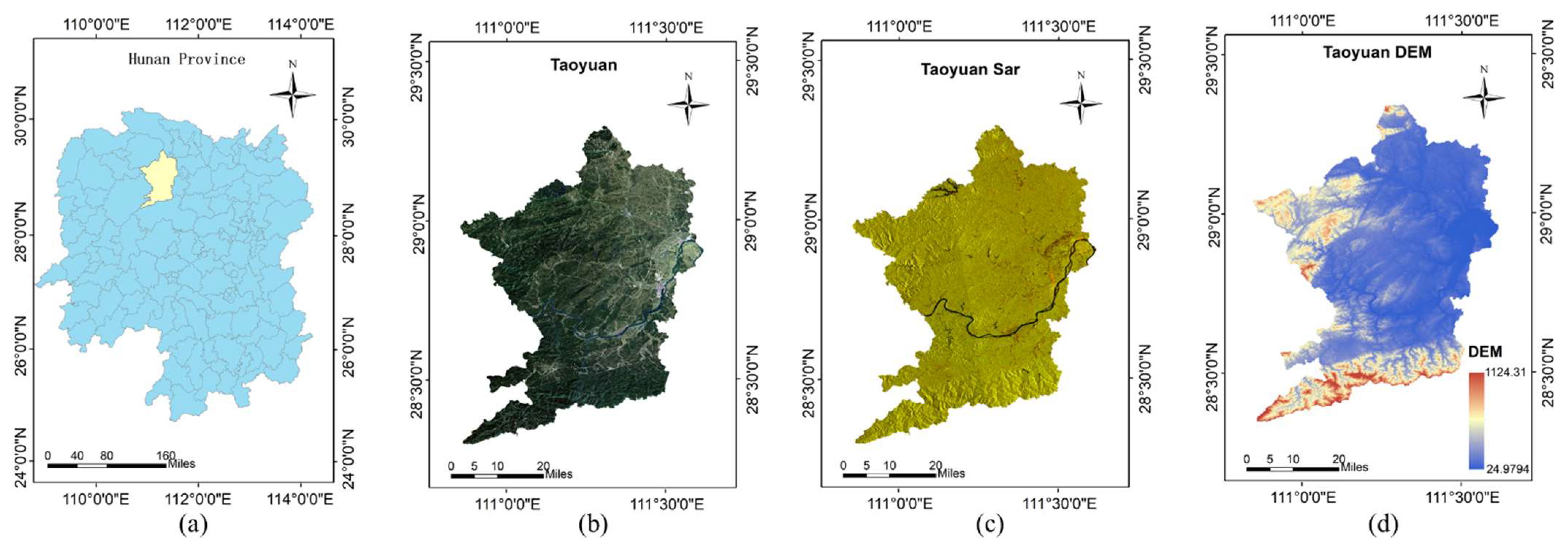
The study area of this work is Taoyuan County in northwestern Hunan Province, China, which is a central town with typical complex geomorphology. Taoyuan County is part of the central Hunan hills and is on the transition zone from the western Hunan mountains to the lakeside plain of Dongting Lake, with a steep western and eastern terrain, high in the north and south, and low in the middle. Most county surfaces are covered by forest land, with forest land accounting for about 70% and construction land accounting for 2%. The remaining surface area is covered by agricultural land and water bodies.
2.2. Data Source
2.2.1. Remote Sensing Data
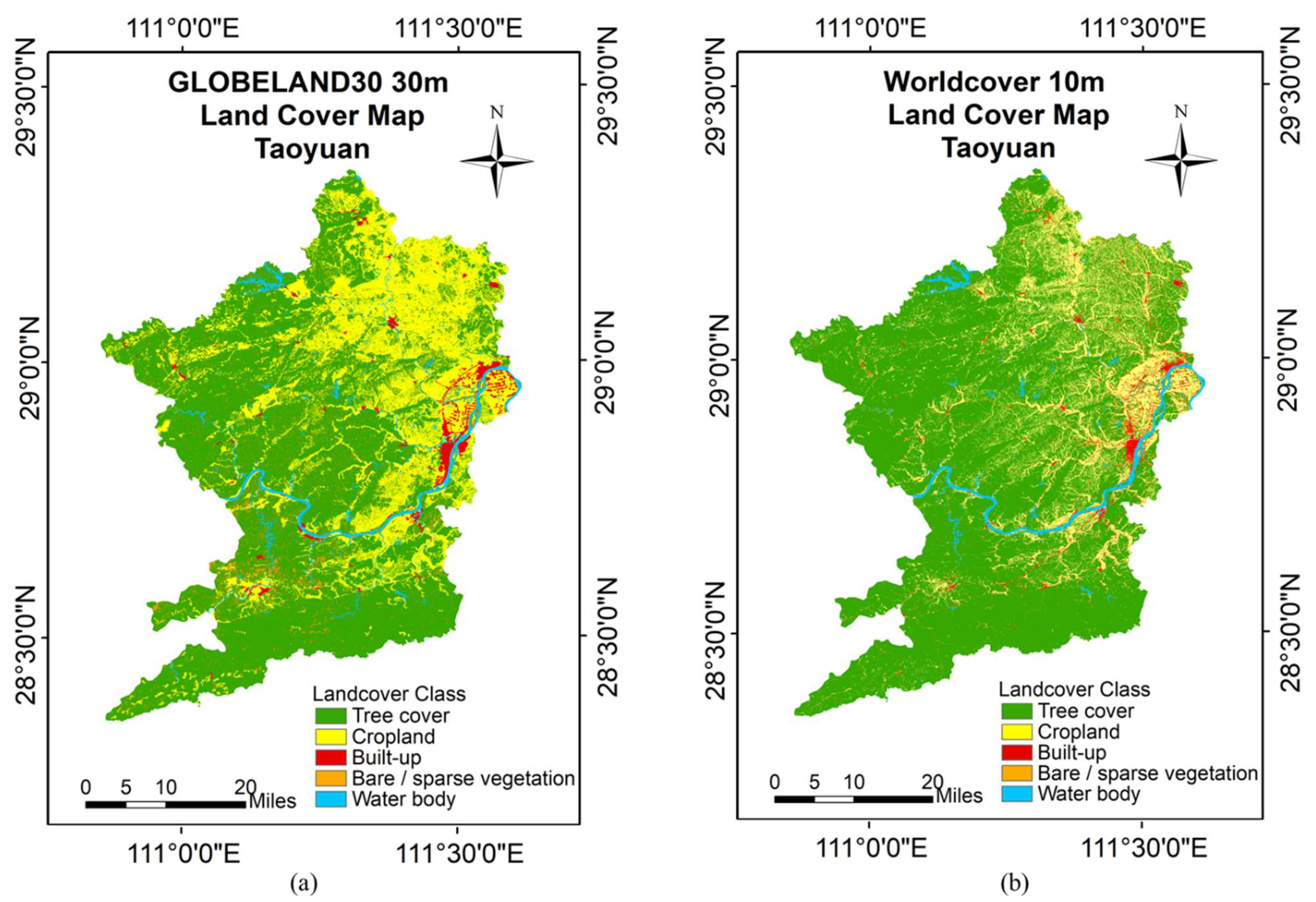
The 10 m resolution remote sensing image of Sentinel-2 was used as the image data for land cover classification. Sentinel-2 L2A level data were downloaded from Google Earth Engine for September 2020 with a spatial resolution of 10 m. Sentinel-2 L2A level data is a geometrically corrected, atmospherically corrected and radiometrically calibrated product released by the European Space Agency (ESA). In this study, the 10 m resolution Sentinel-2 L2A of Taoyuan County in the RGB band image was used as the classification data, as shown in Figure 1. The 2020 globeland30 product [55] of Taoyuan County area was downloaded from the GLOBELAND30 website [74] for the training samples, which provides land cover labels of Taoyuan County at 30 m resolution, but the build-up land category is relatively coarse and a gap with the real land cover can be observed, as shown in Figure 2a. In addition, the 10 m land cover data [54] of Taoyuan County in 2020 were downloaded from the ESA website [75] and used to create a test set for the validation of the algorithm, as shown in Figure 2b. The distribution of farmland and forest land categories on the land cover maps of the two resolutions differs in Figure 2, and the labels of these two categories are easily confused with each other due to a large amount of noise. Meanwhile, the 30 m land cover map has rough build-up land boundaries compared with the 10 m land cover map, and each build-up land area is larger, while other land cover categories exist within the 30 m build-up land spot. Therefore, the labeling of built-up land using the 30 m land cover map will inevitably generate category noise.
2.2.2. Sample Collection
To create the training set, the 30 m resolution land cover label map was resampled to a spatial resolution of 10 m using ArcGIS resampling tool, which enables the 30 m resolution label map to be spatially aligned with the 10 m image. Then, 4000 pixels of build-up land category and 4000 pixels of forest land, waterbody, farmland, and other categories were randomly selected within the whole image with a 30 m resolution land cover as category labels. Subsequently, in order to preserve the contextual information of the selected pixels, 4000 patches of 64 × 64 size are cropped with the selected pixels as the center and added to the training set, and the category of the patches depends on the category of the center pixel. Another advantage of using this method is that each pixel of the remote sensing image of Taoyuan County can be used as the center pixel of the mapping sample, and the pixel-level mapping results can be obtained in the final mapping stage. Since the pixels are randomly selected in the category, if the selected pixels are close enough, a partial overlap is created when cropping the patches. In making the test set, 8000 pixels of build-up land category and 8000 pixels of other categories were randomly selected within the whole image with a 10 m resolution land cover category as the label. The same size patches were cropped out. Considering that less category noise exists in the 10 m land cover product, 4000 construction land categories were selected among the 8000 real samples, and 4000 samples of other land cover types were regarded as the test set. When the 30 m land cover product is used as a label for the 10 m image, the erroneous label category will be brought to the pixels of the 10 m image, and this produces category noise labels. In addition, the 30 m land cover product cannot be guaranteed to be accurate at the time of production, and the same category noise exists due to the misclassification. In this case, the training set produced in this work is a training set containing category noise.
3. Method
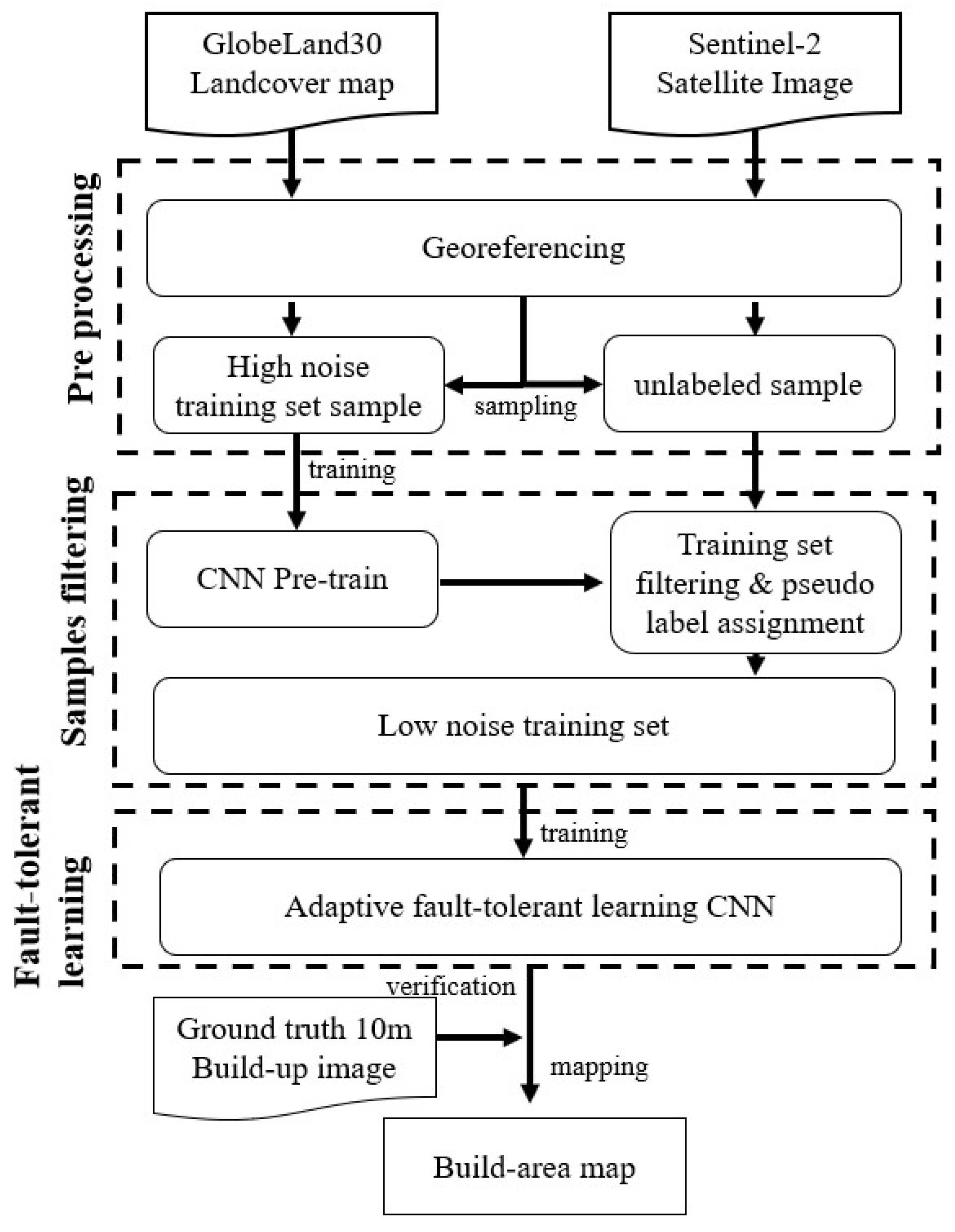
One pixel at 30 m resolution corresponds to 3 × 3 pixels at a 10 m rate due to the difference in resolution. These 9 pixels can only be given category labels of the same pixel from 30 m resolution when using the training set for manufacturing construction land category labels at 30 m resolution for construction land mapping at 10 m resolution. However, the land cover categories of these 9 pixels are not exactly the same in the actual 10 m resolution case. Consequently, the training set will contain incorrect labels (i.e., noisy labels). The goal of the method in this work is for the classifier to find the incorrect labels and learn against the correctly labeled samples in the case that the training set contains noisy labels, allowing the corresponding features of the correct class to be learned, and the images with 10 m resolution can be correctly classified. The flow chart of the method in this work is shown in Figure 3, which includes three steps. First, the land cover map and remote sensing images are preprocessed. Second, the pre-trained baseline is used to calculate the classification confidence of the unlabeled data and filter the samples with higher confidence in the building category to join the new training set for initial noise filtering. Finally, the filtered samples are trained using the fault-tolerant learning loss, and the build-up land mapping results are obtained after verifying the accuracy.
3.1. Problem Formulation of Fault-Tolerant Learning
We suppose that remote sensing image land cover categories with category classes are present in the training set, and each land cover category can be represented by feature type. Let be the feature space of the land cover category, and be the label space. We assume that all the labels are one-hot vectors and use to denote a one-hot vector corresponding to class . Let be the independently and identically distributed samples obtained according to the distribution of . The task of land cover classification is to train the classifier to learn the pattern of distribution using as the training set. However, there is no such training set when using 30 m resolution land cover category labels for land cover classification of 10 m resolution remote sensing images. Instead, the training set is obtained, and is obtained based on the distribution . Here, denotes the incorrect label, and denotes the correct label. and are correlated, and their relationship can be expressed as follows:
where denotes the noise rate, which is the probability that the label becomes . This general model is called class conditional noise because the probability of a label error in this model depends on the original label class. A special case of this model is called symmetric noise. The probability of converting a class label to any other class label is equal in the presence of symmetric noise (i.e., assuming that and , where denotes the probability of a class label error). If all samples labeled by a particular category are selected from the training set of label errors under the condition that , then the samples that really belong to that category are still in the majority in the set.
Now, the fault-tolerant learning problem of build-up land classification under noise labels can be formulated as follows: The build-upland classifier needs to learn the pattern of distribution . However, the training set can only be obtained from the distribution containing the error labels. In the build-up land classification task, let the function of the classifier be , where is a parameter. Assuming that the softmax output layer is used as the last layer of the neural network classifier, the labels of the training samples are all one-hot vectors when the training set is used for training. is a probability vector of the same length as . Thus, the loss function of the classifier in the training phase can be defined as .
3.2. Training Set Sample Filtering and Pseudo-Label Assignment Method
The presence of category noise in the training set leads to a degradation of the classification performance. Accordingly, direct training with training sets containing a large amount of noise does not achieve satisfactory accuracy. We propose a semi-supervised learning scheme for confidence-based filtering of unlabeled remote sensing images to produce a low-noise dataset in this work to obtain datasets containing less noise, which is inspired by the pseudo-label assignment strategy [76] for obtaining valuable samples and the joint fine-tuning strategy [77] for using high-confidence samples to participate in optimization. The idea of the pseudo-label assignment is to select valuable samples based on the predicted classification confidence [76]. However, these pseudo-labels may not be reliable. Joint fine-tuning optimizes the classification model by adding samples with high confidence in the training set [77], but it requires a small number of labeled samples. Our solution combines the advantages of the above-mentioned two approaches to obtain reliable training information from unlabeled data for low-noise dataset construction for model optimization.
In a given training set , we input each patch into the baseline for pre-training. The output vector of the softmax layer is the confidence given by the classifier for the class to which belongs. This vector is denoted by using , where denotes the confidence that patch belongs to category c, and C is the total number of categories. We can use the confidence level to determine whether an unlabeled sample is associated with a label because the baseline has a strong discrimination ability.
After inputting unlabeled samples into the pre-training model, the first step is to rank the maximum value of the confidence level of each category to which the unlabeled patch belongs. In a given filtering threshold [0, 1], the N× samples with the maximum confidence level are selected to be added to the new training set, and the maximum value in is used for the samples assigned with category labels. The filtering threshold can be set based on the results of the pre-training test precision, which is also a response to the category labels in the samples. If the precision is low, indicating that the sample contains more noise, then should be reduced to obtain samples with better confidence; if the precision is high, indicating less noise in the sample, then can be appropriately increased. However, the precision should not be set particularly large. A large will bring in many noisy samples and weaken the effect of sample filtering.
3.3. Adaptive Fault-Tolerant Curriculum Learning Based on Batch Statistics
Curriculum learning can be considered a minimization of weighted losses [78]:
where represents the curriculum. b is selected here as the size of a minibatch because the optimizer generally chooses SGD in the learning process. A simple choice for this curriculum is . Substituting this equation into Equation (2) and taking and considering the case where λ depends on the category label, Equation (2) can become:
Where . In any fixed , the optimal solution of the optimization problem is given by the relation: when , the optimal solution ; when , the optimal solution , with . Moreover, this relationship holds even when is a function of or a function of all samples in the data set that matches . Then, a truly dynamically adaptive optimization problem is available for the curriculum (i.e., by letting depend on all in the minibatch and on the current value of ).
In the choice of threshold , consider those samples with no errors in the labels for satisfying , and can be set to update in minibatches when . Given enough empirical evidence that samples with correct category labels are easier to learn than those with noise, some quantiles of the set of loss values obtained in small batches quantile or a similar statistic would be a good choice for .
We can obtain because we use cross-entropy loss. is the posterior probability that belongs to class at current because the network has a softmax output layer. The criterion for choosing the threshold can be that the assigned posterior probability is higher than a threshold value because the loss value and this posterior probability are inversely proportional. The method threshold in this work is set to the mean value of the posterior probability of each category of samples in a minibatch because the mean value can represent the confidence level of most of the samples in this category.
The above-mentioned method of learning adaptive fault-tolerant curriculum based on batch statistics can become:
where mean denotes the sample mean of the category posterior probability of the samples with category label , where denotes the number of all category samples in the minibatch.
Considering that the neural network is trained using minibatches, the algorithm consists of three parts:
- Calculation of the sample selection threshold for a given small batch of data;
- Sample selection based on the threshold and Equation (4);
- Network parameter update using these selected samples.
4. Results
4.1. Experimental Settings
In view of the different sizes and scales of buildings, this study uses a multi-scale classification model for remote sensing image feature extraction and classification. The model consists of four convolutional modules and four fully connected layers. The maximum pooling operation is also added in the second and fourth convolutional modules. The RELU activation operation is added in the fully connected layer, and the dropout is used to prevent overfitting. The input of the model is a mini-patch of 64 × 64, 32 × 32, and 16 × 16 size of the same patch for multi-scale feature extraction, and the specific structure of the CNN is shown in Table 1. The experiments will use the multiscale classification model with cross-entropy loss as the baseline.
This experiment uses the Pytorch deep learning framework, which is trained on a computer with NVIDIA RTX3090 GPU, Intel i9-10900KF CPU, and 32 GB RAM. The training epoch is set to 1000, the batch size is set to 64, and the initial learning rate is 10-3. When the loss stops decreasing, we divide the learning rate by 10 and update the parameters with a new value. Pre-training is carried out using the training set before filtering, and the unlabeled samples are filtered by setting the hyperparameter σ according to the test accuracy of pre-training. Then, the 10 m image samples filtered by confidence are trained, mapped in the whole area of Taoyuan County, and tested with the artificial ground real data.
4.2. Evaluating Indexes
The widely used overall accuracy (OA), confusion matrix (CM), and Cohen’s Kappa coefficient are applied to evaluate. In addition, the producer’s accuracy and user’s accuracy are also calculated.
CM is a matrix of n rows and n columns to represent the classification effect, where each row represents the actual category and each column represents the predicted value. It can indicate the categories that are prone to confusion, thus more intuitively representing the performance of the algorithm.
The formulas of OA and kappa coefficient are as follows:
where n represents the category, N represents the sum of the number of samples, represents the diagonal elements of the confusion matrix, represents the sum of the columns of the category, and represents the sum of the rows of the category.
4.3. Mapping Results
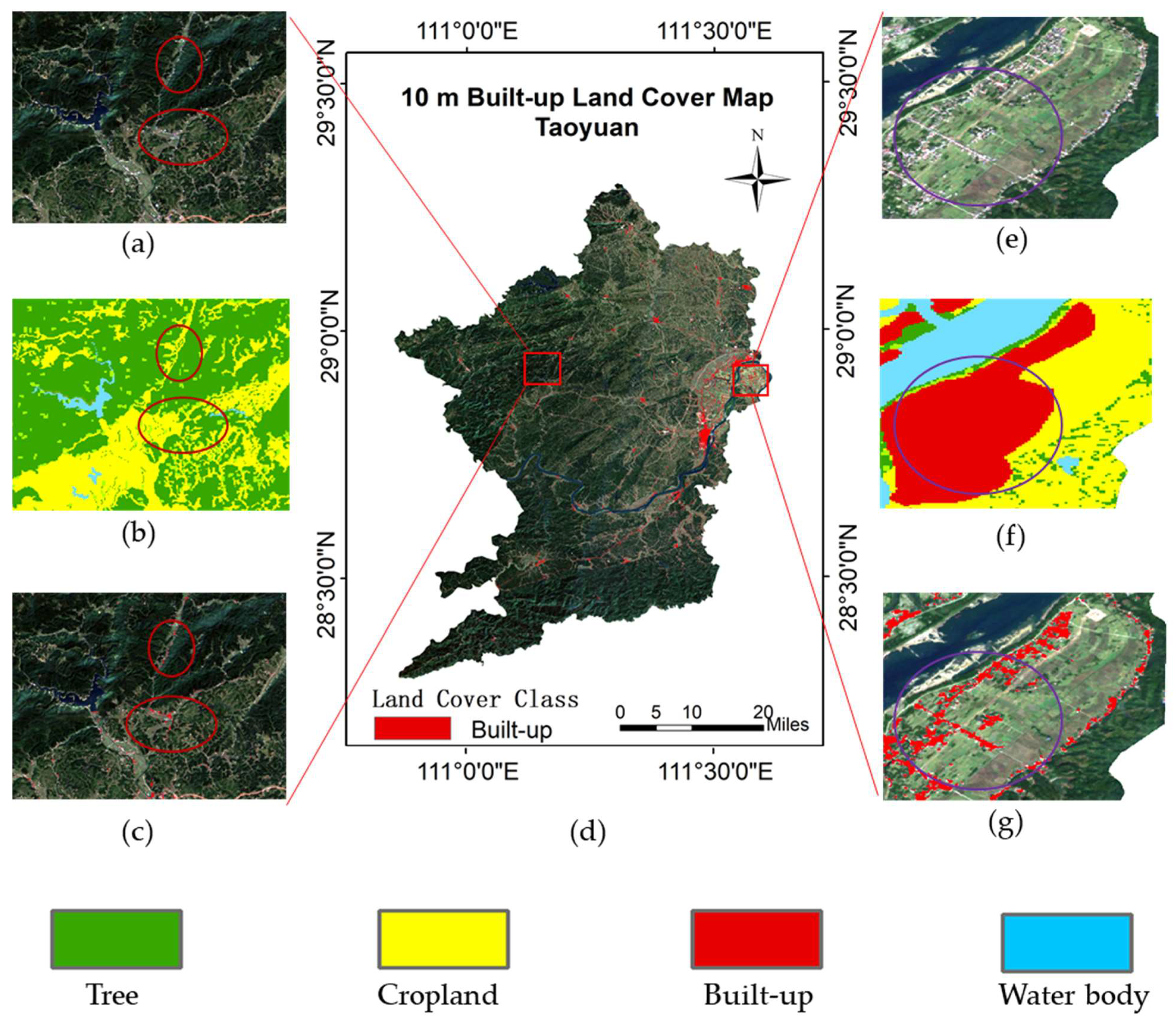
The 10 m resolution build-up land mapping of Taoyuan County in 2020 is shown in Figure 4d. The overall results of construction land extraction in Taoyuan County in 2020 are good, and the boundaries of construction areas are more detailed compared with the 30 m land cover map, as shown in Figure 4. Large areas of construction land can refine the boundaries of build-up land and distinguish the internal non-build-up land areas, as shown in Figure 4e–g. The present mapping method can also find smaller settlements and even single-family houses, indicating that this method can help us in accurately understanding the urban expansion and land use changes, which is difficult to achieve with 30 m land cover maps (Figure 4a–c). Another major advantage of this method is the ability to use the trained model for construction land mapping of the latest image products to obtain the latest information on build-up land because the temporal coverage of the 10 m product data is not extensive.
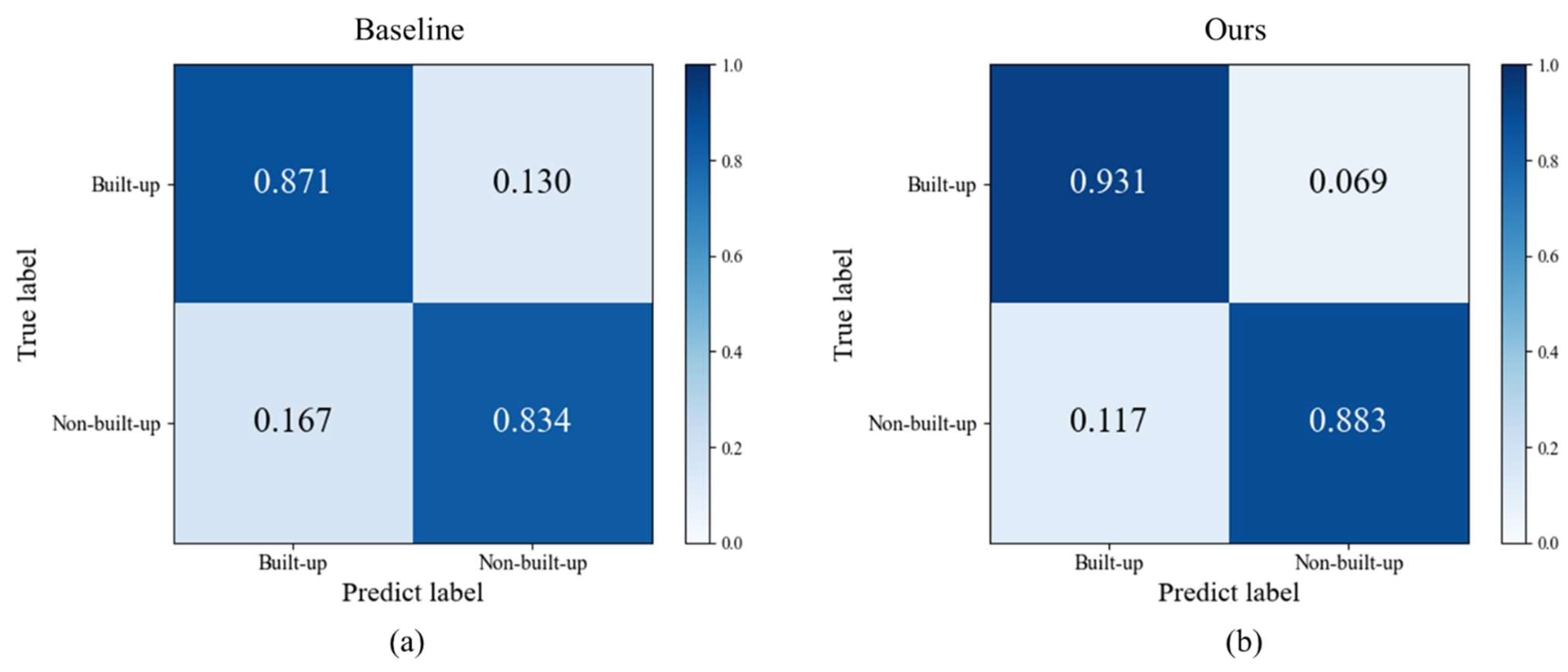
Table 2 shows that our method improves OA by 5.5%, Cohen’s Kappa coefficient by 0.11, producer’s accuracy by 4.9% and user’s accuracy by 6% over the baseline, which is the average result obtained by conducting 10 replicate experiments. This result shows the effectiveness of our method in classifying the build-up land in Taoyuan County. Moreover, this result verifies that category noise is generated when using the 30 m land cover map as a label for the 10 m image. The confusion matrices are shown in Figure 5.
4.4. Generalizability Assessment
The sample filtering in this method is assigned based on the confidence level of the unlabeled samples in the pseudo-label assignment method. The unlabeled samples from different regions can be added to the sample set to be filtered for filtering to improve the generalizability of the model. In this part of the experiment, we do not change the pre-training sample set. Only the set of unlabeled samples to be filtered is changed using the Sentinel-2 L2A cloudless images in September 2020 of Taojiang, Anhua, and Xinhua counties, which are geographically adjacent to Taoyuan County and have similar surface coverage types, to crop a total of 24,000 unlabeled image patches of 64 × 64 size and add them to the sample set to be filtered. After the sample screening and fault-tolerance training, the generalization of the method was verified by creating a test set with the 10 m land cover of the four counties for the build-up land category.
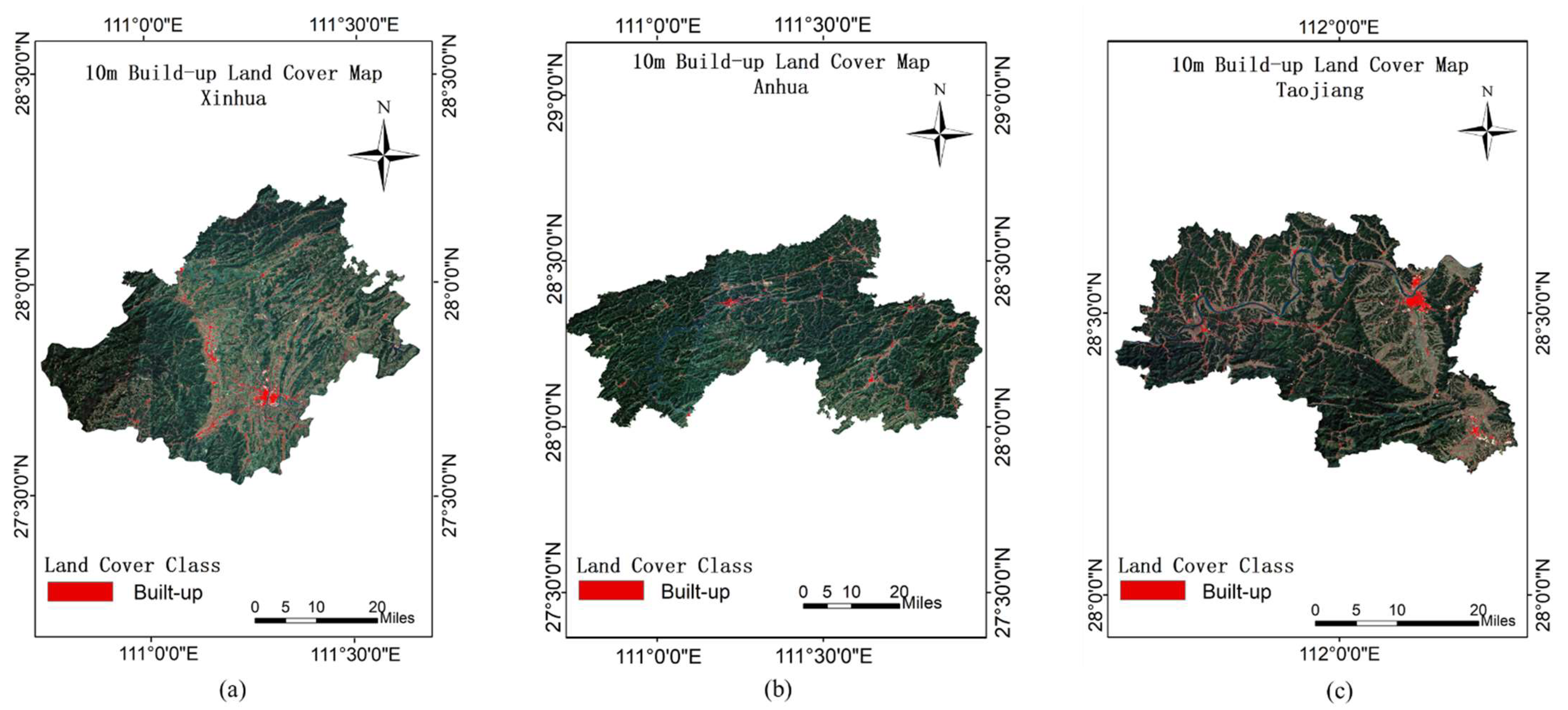
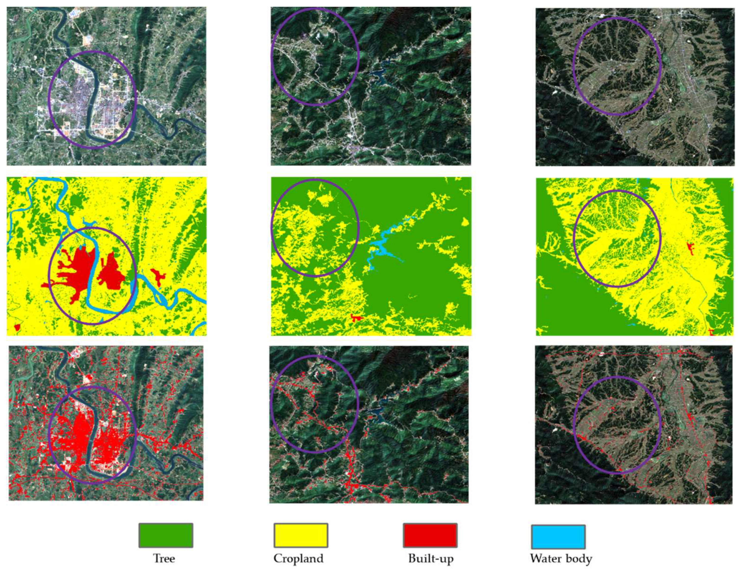
The results of build-up land mapping in Taojiang, Anhua, and Xinhua counties are obtained according to the experimental method in Section 4.4, as shown in Figure 6. Figure 7 shows that the build-up land mapping results of Taojiang, Anhua, and Xinhua counties can also reflect the fine town boundaries and smaller area of settlements and single buildings. Better results are obtained in different scenes, such as farmland, woodland, and urban areas, which are more fine compared with the 30 m land cover resolution.
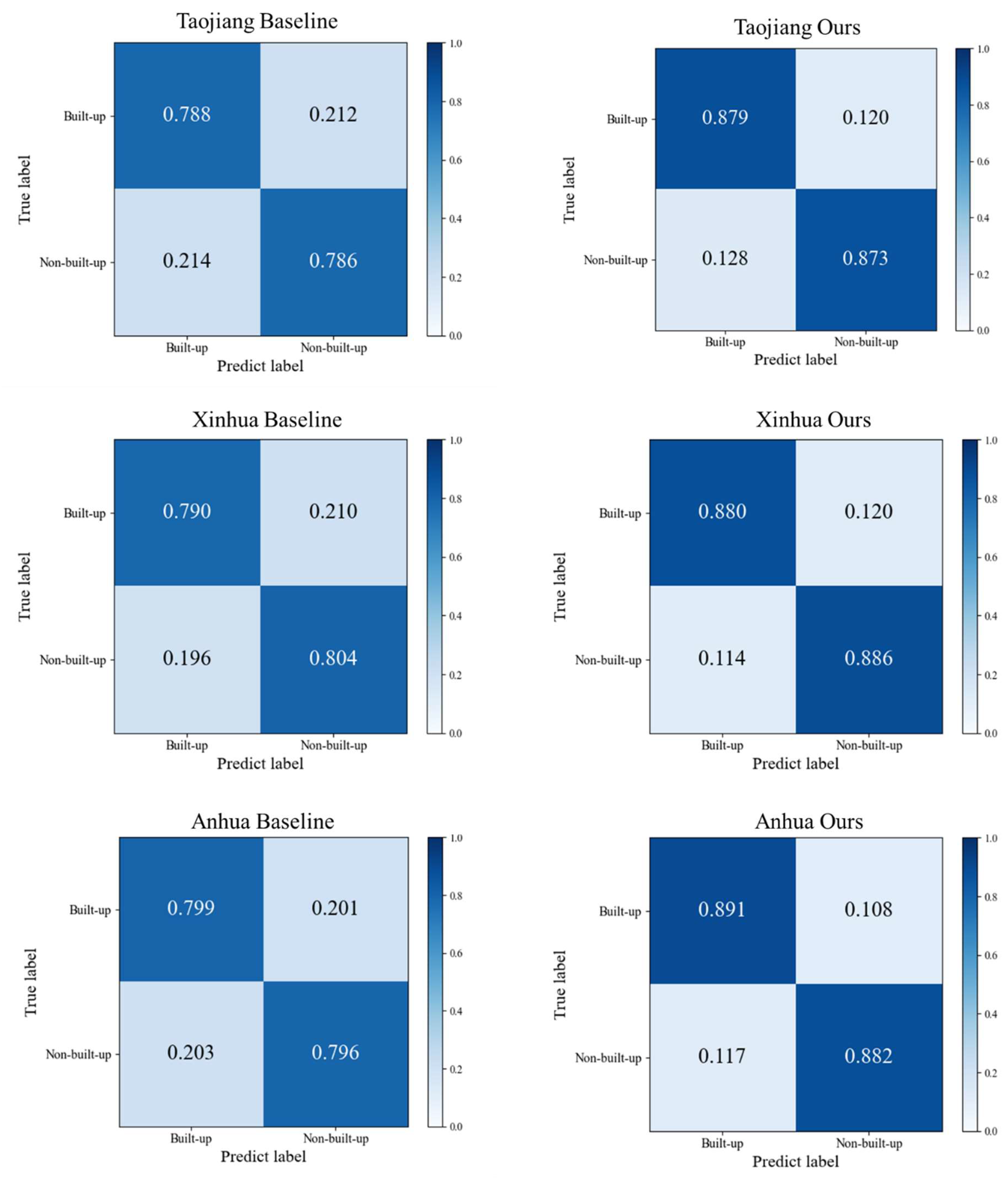
The method can efficiently perform on the data of all four counties, as shown in Table 3. The average OA accuracy reaches 88.2% and average Cohen’s Kappa reaches 0.588 without changing the pre-training set and using the unlabeled samples obtained from remote sensing images of the four counties for filtering and fault-tolerant training, indicating that the method is able to perform more accurate build-up land mapping and has better generalizability. However, the baseline obtained by simply using the training set of Taoyuan County, which contains more category noise, was tested on the image data of four counties without filtering and expanding the unlabeled samples, and the average OA accuracy was only 79.4%, indicating that the generalization of the baseline is insufficient. Among the results for each county, using this method Anhua County obtained relatively low accuracy results relative to the other two counties, which may be due to the fact that the built-up area in Anhua County is smaller in number and scope compared to Taoyuan County, producing a certain degree of difference from Taoyuan County. As can be seen from the confusion matrices in Figure 8, the confusion of our method is lower than that of baseline.
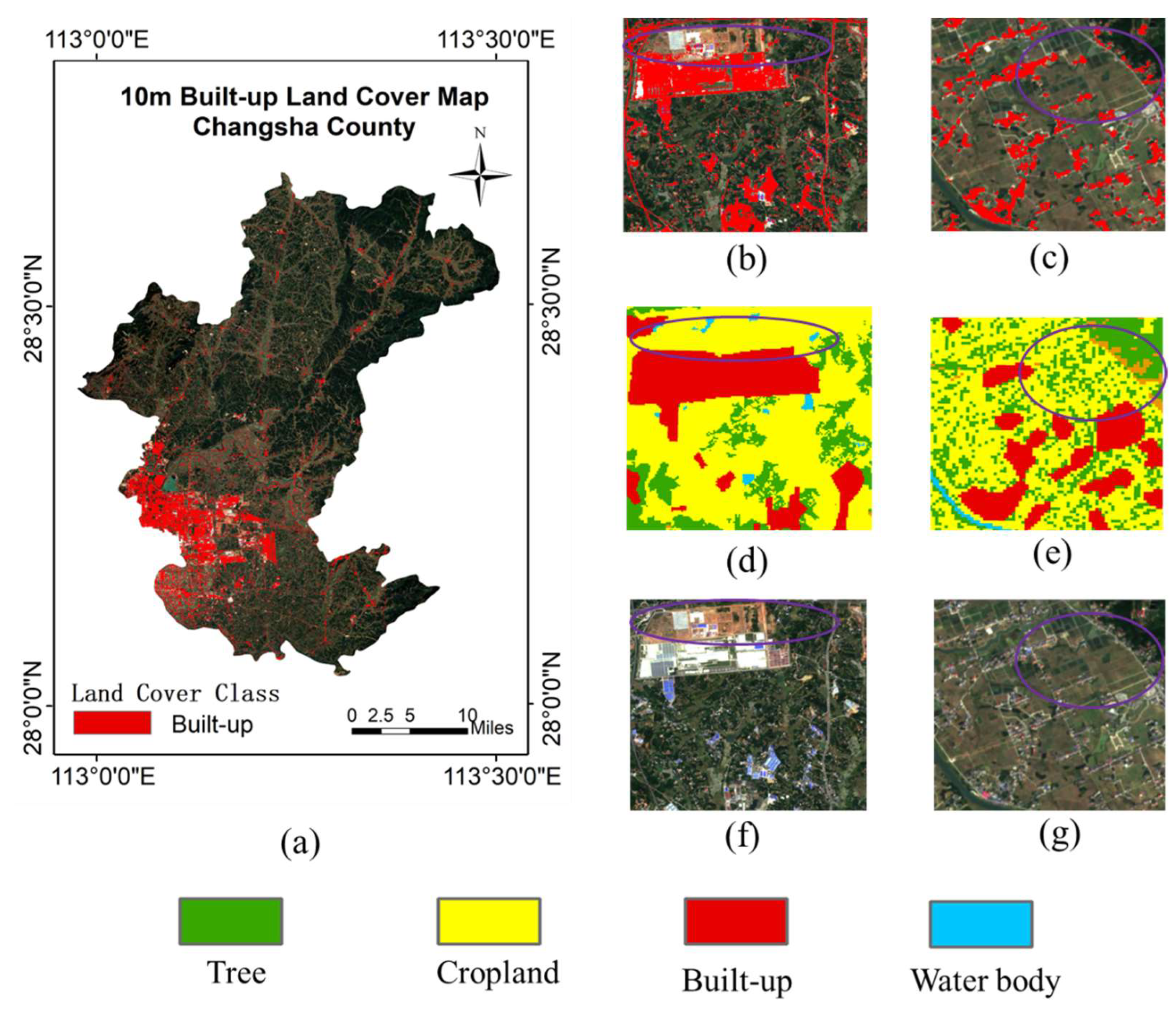
In addition, to evaluate the cartographic effect of the model in areas with different urbanization processes than Taoyuan County, we selected the cloudless Sentinel-2 images of Changsha County in September 2020 for evaluation. Changsha County is part of Changsha City which is the capital of Hunan Province, and is one of the top ten economic counties in China. Changsha County is close to Changsha City, with a large population and developed industries. The built-up area of the county is large and widely distributed, and the land cover is dominated by plains, with the terrain gradually sloping from the north, east and south to the central and west. Similarly, we do not change the pre-training sample set, but only the unlabeled sample set to be screened, and use the Sentinel-2 L2A images of Changsha County to crop a total of 8000 unlabeled images of 64 × 64 size patches to be added to the sample set to be filtered, and then complete the sample filtering and fault-tolerant training model to obtain the validation results as shown in Table 4, the mapping results as shown in Figure 9 and the confusion matrices as shown in Figure 10.
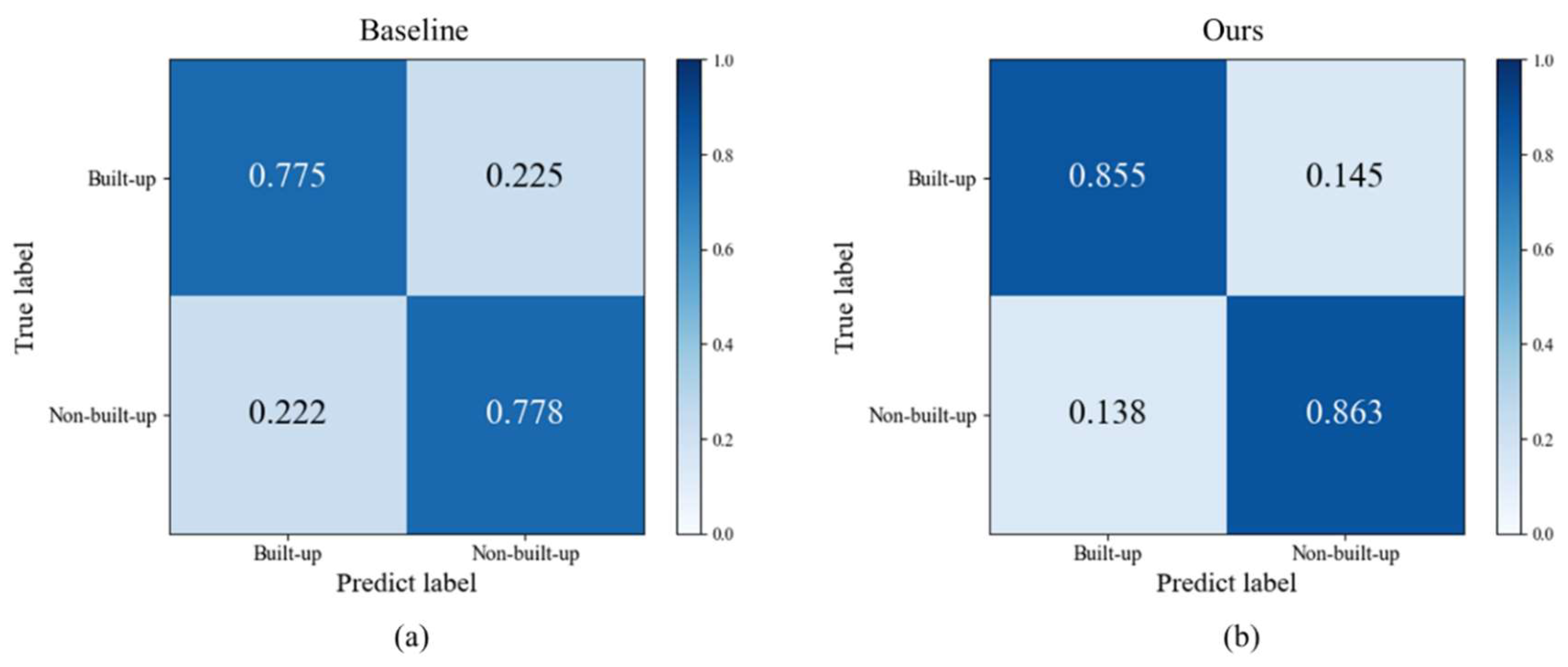
As shown in Table 4, in Changsha County, where the urbanization process is different from Taoyuan County, the OA of our method reaches 85.9% higher than baseline by 8.2%, and Cohen’s Kappa is 0.718 higher than baseline by 0.164, indicating that the method has better generalization and achieves in areas with different urbanization process satisfactory results. Figure 9c,e,g show the advantages of the model in extracting small area settlements. Additionally, Figure 10 shows our methods is better than baseline. However, the results of our method in Changsha County are 2.3% lower than the average OA of Taojiang County, Xinhua County, and Anhua County, indicating that the urbanization process, differences in the extent and size of building sites, and the distribution of land cover types may have an impact on the results. As in Figure 9b,f, some of the building sites exhibit white and blue roofs, but are not well extracted. The reason for this result may be that there is a difference in the distribution of construction land types in Changsha County, which is industrially developed with many factories, but Taoyuan County is not.
4.5. Applications for Future Scenarios
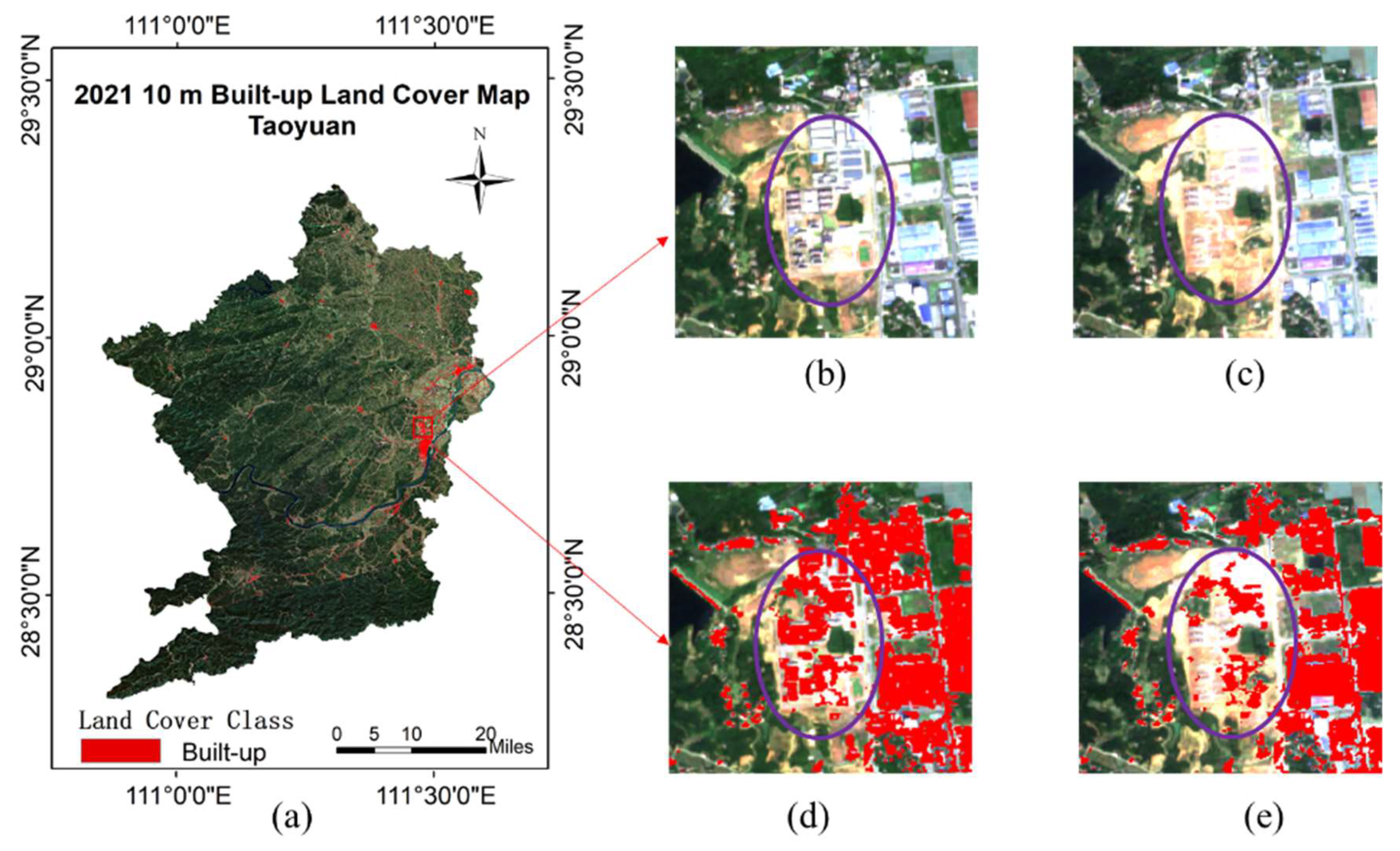
Urbanization is growing rapidly, and construction land maps need to be updated rapidly to meet the needs of the industry. Therefore, one application scenario of our method is to use the model trained from existing data for built-up land mapping of future images to update existing maps. We acquired cloud-free Sentinel-2 L2A level images of Taoyuan County in September 2021 from GEE. After cropping 8000 patches of 64 × 64 size, they were input to the pre-trained sample filtering and pseudo-label assignment model for Taoyuan County in 2020, and confidence sample filtering and label assignment values were performed for 8000 patches in 2021 to build a training set for fault-tolerant training.
For the test data, the surface coverage labels could not be obtained due to the lack of 10 m land cover products for 2021 in Taoyuan County, but considering that the time period of image acquisition is only 1 year different, the acquisition season is the same, and the built-up land in Taoyuan County does not change to a large extent within 1 year, the test set built with the 2020 data in Section 2.2.2 is still used for testing. In addition, since training on baseline requires the land cover map as the label, this section was not experimented on baseline. The mapping results are shown in Figure 11, and the test results are shown in Table 5 and Figure 12.
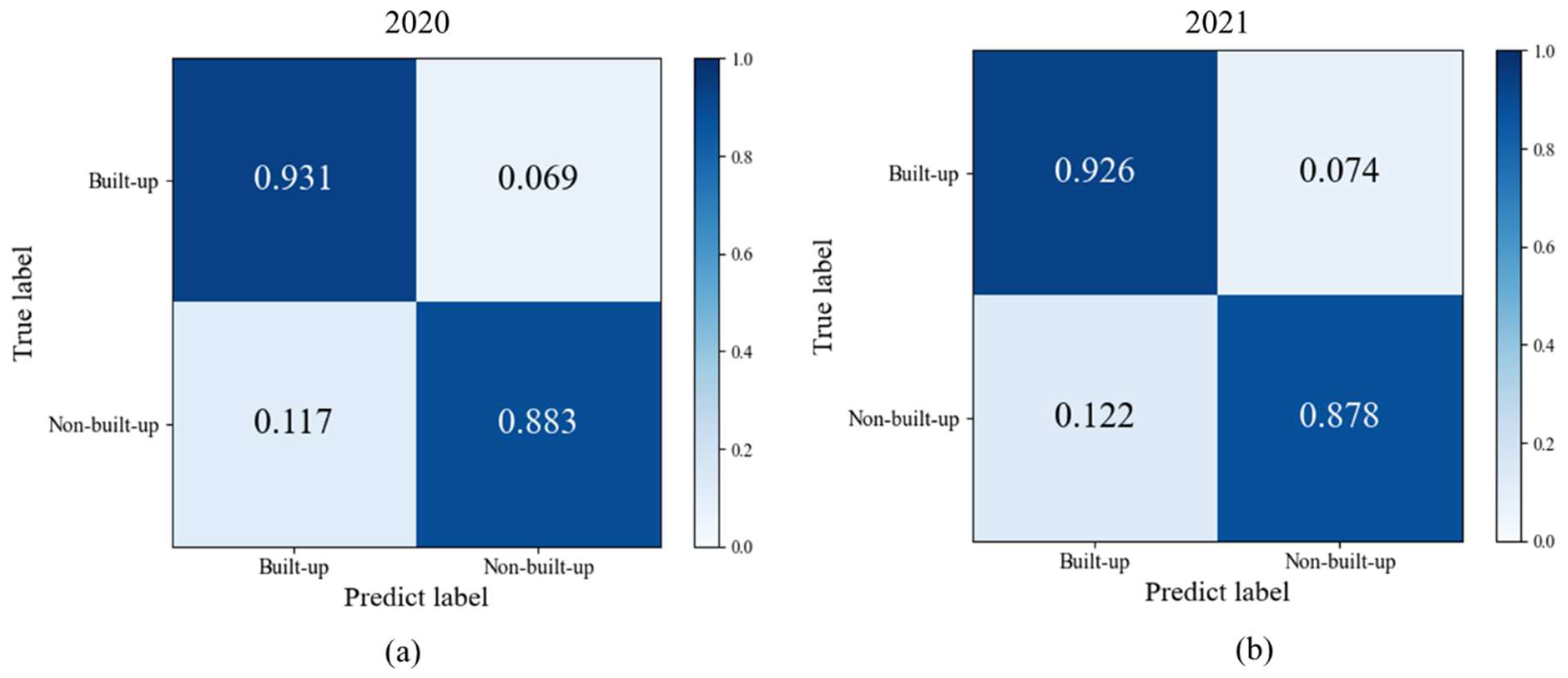
As shown in Table 5, the overall accuracy OA of Taoyuan County reached 90.2% in 2021, which is only 0.5% less OA compared to 2020, Cohen’s Kappa decreased by 0.01, producer’s accuracy decreased by 0.4%, and user‘s accuracy decreased by 0.5%. As can be seen from Figure 11, the model can also detect the newly added built-up land in Taoyuan County. Therefore, the model can be better applied to future data for fast update of construction land use maps.
5. Discussion
5.1. Evaluation of the Effects of SF and AFCB
SF denotes the training set sample filtering and pseudo-label assignment method, and AFCB denotes the adaptive fault-tolerant curriculum learning method based on batch statistics. Four sets of experiments are conducted in this section, which are:
- The baseline model uses cross-entropy loss and multiscale network.
- Baseline and training set sample filtering scheme are used.
- AFCB and multiscale network are used.
- The training set sample filtering scheme and AFCB are used. The experimental results are shown in Table 6.
Table 6 demonstrates that the training sample filtering can yield satisfactory results, improving the OA accuracy by about 3%, and using AFCB alone is also able to improve OA accuracy by 2.5%. The noise learning strategies used in this study worked. Finally, we are able to improve the OA accuracy by 5.5% over baseline by using both methods. The OA accuracy reached 90.7%, and this accuracy can support us in producing the build-up land map.
5.2. Band Evaluation
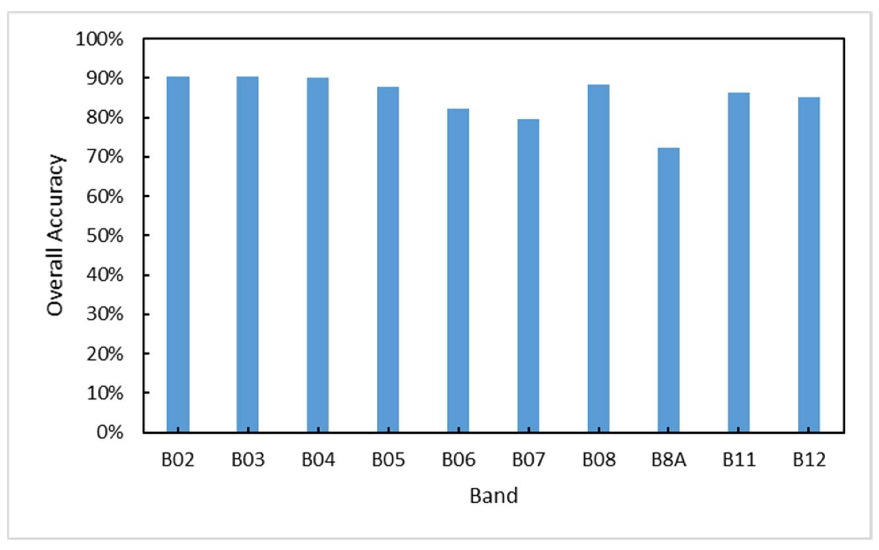
In this paper, we use the RGB bands of Sentinel-2 data for built-up land mapping, but there are 13 bands in Sentinel-2 data (Table 7). Therefore, in order to evaluate the validity of the bands, we acquired seven other bands from GEE that are applicable to land cover classification in the same L2A level image as the Sentinel-2 RGB image in 2.2.1. (The other three bands, B01, B09 and B10 are intended for atmospheric correction and therefore not considered.) Evaluating using single-band images as well as shortwave-infrared (SWIR) and red edge bands combinations on our method. We use a cubic spline interpolation [79] method to upsample the 20 m spatial resolution band to 10 m. The sampling and training methods are the same as above using RGB images. Figure 13 shows the comparison of the performance of each spectral band. Table 8 shows the results for the band combinations. The results show that the single-band performance of the R, G, and B bands outperforms the other bands. The results of band combinations are better than the results of single bands. Additionally, RGB band combination is the best for construction land classification, which is consistent with the results of [51].
In addition, there are more studies using SAR data fused with optical data for surface coverage classification [48,80,81]. Therefore, to evaluate whether the fusion of SAR data can improve the performance of the method, we obtained VV and VH data from GEE with a spatial resolution of 10 m for the Sentinel-1 c-band in September 2020, which was processed by thermal noise removal, radiometric calibration, terrain correction and the final terrain-corrected values are converted to decibels via log scaling (10 × log10(x)). Since RGB works best in the band combination experiment, we then changed the number of input channels of the CNN model to 5 and produced images of five channels of R, G, B, VV, and VH and sampled and trained them using the same method as above. The testing results are shown in Table 9. The results show that the accuracy of the results using RGB+SAR data fusion is 0.2% lower than that using only RGB optical data, which may be due to the fact that the fusion effect of optical and SAR data depends on the classifier, and better performance may not be obtained using CNN [48,81].
5.3. Testing of Ground Truth Data
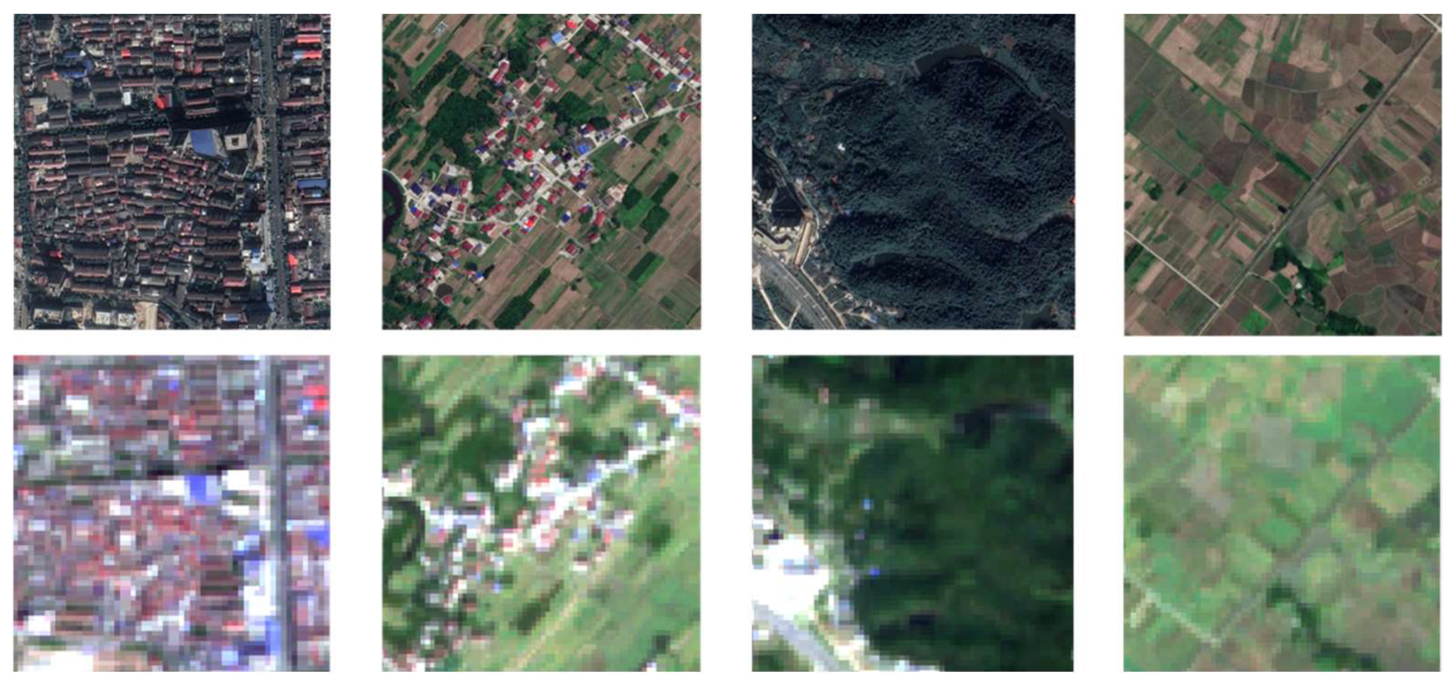
The advantage of the method in this paper is the ability to quickly obtain high-resolution built-up maps using publicly available data products, so the test set labels used are from the global 10 m land cover product. However, due to the uncertainty in the global 10 m land cover product itself, it may still exist despite sample selection to reduce the uncertainty. Therefore, in order to assess the uncertainty of the method in this paper, we use sub-meter high-resolution remote sensing image data from Google Maps to label ground truth samples of built and non-built land in Taoyuan County. By using visual interpretation and map annotation tools, we annotated 200 built-up land points and 200 non- built-up land points. Additionally, with 400 points of latitude and longitude as the patches’ center, the RGB image of Sentinel-2 in 2020 was cropped to 64 × 64 size patches, so that we obtained 200 ground truth samples of construction land and 200 non-construction land, as shown in Figure 14.
Tests were performed on the model of our method using 10m land cover products and ground truth data and the results are shown in Table 10. As can be seen from Table 10, there is only a slight difference in the performance of the model on the test set produced by the 10m land cover product and on the ground truth, whether using the baseline or our approach. The possible reason is that both the production of WorldCover land cover products and the extraction of built-up land in Taoyuan County in this paper use the 2020 Sentinel-2 images as data sources, and the confused categories of built-up land in the products are bare lands and grasslands [54], while most of the areas in Taoyuan County are covered by trees and croplands. Therefore, for the construction land, the uncertainty in the land cover product can be basically ignored, and it can be used as a reliable substitute for the ground truth data in the absence of ground truth data.
6. Conclusions
In this work, we convert the mapping results of land cover at 30 m resolution to build-up land mapping at 10 m resolution. The research method in this work is a new solution that can accomplish this work without human effort. Our proposed build-up land mapping method is able to achieve high accuracy in the case of labels containing category noise due to its better denoising and fault-tolerant capabilities. We obtained construction land mapping results with higher resolution than 30 m and 90.7% accuracy by using 30 m land cover category labels to learn from 10 m images. Our proposed solution uses training set sample filtering and pseudo-label assignment to accomplish the filtering of high-confidence samples and filter out a portion of noisy samples. The adaptive fault-tolerant curriculum learning method based on batch statistics used in the method further filters the samples with relatively correct labels during the training process. The combined use of the two strategies improves the overall accuracy by 5.5%. In addition, our proposed method has good generalizability and can be adapted to regions with similar land cover classes. Our method demonstrates the possibility of extending from existing low-resolution map products to high-resolution map products and can significantly reduce the human and material resources consumed in performing such mapping efforts, providing time-sensitive data support for urbanization.
However, the method also has shortcomings. If the noise in the sample is considerably large, then a good pre-training effect will be difficult to achieve, and the sample selection will be a challenge due to the limitation of the method. Considerable noise will also make it difficult for the batch statistics to reflect the true category mean value, resulting in the failure of the algorithm. The remote sensing data still contains a lot of data with category noise, and fault-tolerant learning strategies have many potential opportunities in remote sensing scenarios. In future research, we will consider adding prior knowledge of categories to reduce the impact of noise labels on the classification models.
Author Contributions
Conceptualization, G.X. and J.C.; methodology, G.X. and G.S.; software, Y.F.; validation, G.X. and Y.F.; formal analysis, G.X.; investigation, M.D.; resources, G.S.; data curation, G.S.; writing—original draft preparation, G.X.; writing—review and editing, G.X. and J.C.; visualization, G.X.; supervision, J.C.; project administration, J.C.; funding acquisition, J.C. All authors have read and agreed to the published version of the manuscript.
Funding
The work was supported by the National Key Research and Development Program of China, Grant 2020YFA0713503; the National Natural Science Foundation of China, grant number No. 42071427.
Conflicts of Interest
All authors declare no conflict of interest.
References
- Wulder, M.A.; Hermosilla, T.; Stinson, G.; Gougeon, F.C.C.O.; White, J.C.; Hill, D.A.; Smiley, B.P. Satellite-based time series land cover and change information to map forest area consistent with national and international reporting requirements. For. Int. J. For. Res. 2020, 93, 331–343. [Google Scholar] [CrossRef] [Green Version]
- Richards, D.R.; Thompson, B.S.; Wijedasa, L. Quantifying net loss of global mangrove carbon stocks from 20 years of land cover change. Nat. Commun. 2020, 11, 1–7. [Google Scholar] [CrossRef] [PubMed]
- Negese, A. Impacts of land use and land cover change on soil erosion and hydrological responses in Ethiopia. Appl. Environ. Soil Sci. 2021, 2021, 6669438. [Google Scholar] [CrossRef]
- Gasser, T.; Crepin, L.E.A.; Quilcaille, Y.; Houghton, R.A.; Ciais, P.; Obersteiner, M. Historical CO2 emissions from land use and land cover change and their uncertainty. Biogeosciences 2020, 17, 4075–4101. [Google Scholar] [CrossRef]
- Qamer, F.M.; Shehzad, K.; Abbas, S.; Murthy, M.; Xi, C.; Gilani, H.; Bajracharya, B. Mapping deforestation and forest degradation patterns in western Himalaya, Pakistan. Remote Sens. 2016, 8, 385. [Google Scholar] [CrossRef] [Green Version]
- Thakur, T.K.; Patel, D.K.; Bijalwan, A.; Dobriyal, M.J.; Kumar, A.; Thakur, A.; Bohra, A.; Bhat, J.A. Land use land cover change detection through geospatial analysis in an Indian Biosphere Reserve. Trees For. People 2020, 2, 100018. [Google Scholar] [CrossRef]
- Radeloff, V.C.; Hagen, A.E.; Voss, P.R.; Field, D.R.; Mladenoff, D.J. Exploring the spatial relationship between census and land-cover data. Soc. Nat. Resour. 2000, 13, 599–609. [Google Scholar]
- Demissie, F.; Yeshitila, K.; Kindu, M.; Schneider, T. Land use/Land cover changes and their causes in Libokemkem District of South Gonder, Ethiopia. Remote Sens. Appl. Soc. Environ. 2017, 8, 224–230. [Google Scholar] [CrossRef]
- Zhang, C.; Wei, S.; Ji, S.; Lu, M. Detecting large-scale urban land cover changes from very high resolution remote sensing images using CNN-based classification. ISPRS Int. J. Geo-Inf. 2019, 8, 189. [Google Scholar] [CrossRef] [Green Version]
- Pauleit, S.; Duhme, F. Assessing the environmental performance of land cover types for urban planning. Landsc. Urban Plan. 2000, 52, 1–20. [Google Scholar] [CrossRef]
- Wang, C.; Wang, Y.; Wang, R.; Zheng, P. Modeling and evaluating land-use/land-cover change for urban planning and sustainability: A case study of Dongying city, China. J. Clean Prod. 2018, 172, 1529–1534. [Google Scholar] [CrossRef]
- Pauleit, S.; Ennos, R.; Golding, Y. Modeling the environmental impacts of urban land use and land cover change—A study in Merseyside, UK. Landsc. Urban Plan. 2005, 71, 295–310. [Google Scholar] [CrossRef]
- Alcantara, C.; Kuemmerle, T.; Prishchepov, A.V.; Radeloff, V.C. Mapping abandoned agriculture with multi-temporal MODIS satellite data. Remote Sens. Environ. 2012, 124, 334–347. [Google Scholar] [CrossRef]
- Ngo-Mbogba, M.; Yemefack, M.; Nyeck, B. Assessing soil quality under different land cover types within shifting agriculture in South Cameroon. Soil Tillage Res. 2015, 150, 124–131. [Google Scholar] [CrossRef]
- Tölle, M.H.; Engler, S.; Panitz, H.U.R. Impact of abrupt land cover changes by tropical deforestation on Southeast Asian climate and agriculture. J. Clim. 2017, 30, 2587–2600. [Google Scholar] [CrossRef]
- Mladenoff, D.J.; Niemi, G.J.; White, M.A. Effects of changing landscape pattern and USGS land cover data variability on ecoregion discrimination across a forest-agriculture gradient. Landsc. Ecol. 1997, 12, 379–396. [Google Scholar] [CrossRef]
- De Faria Peres, L.; De Lucena, A.J.; Rotunno Filho, O.C.E.A.; De Almeida Franca, J.R. The urban heat island in Rio de Janeiro, Brazil, in the last 30 years using remote sensing data. Int. J. Appl. Earth Obs. 2018, 64, 104–116. [Google Scholar]
- Zhang, Z.; Liu, F.; Zhao, X.; Wang, X.; Shi, L.; Xu, J.; Yu, S.; Wen, Q.; Zuo, L.; Yi, L.; et al. Urban expansion in China based on remote sensing technology: A review. Chin. Geogr. Sci. 2018, 28, 727–743. [Google Scholar] [CrossRef] [Green Version]
- Sun, Y.; Zhao, S. Spatiotemporal dynamics of urban expansion in 13 cities across the Jing-Jin-Ji Urban Agglomeration from 1978 to 2015. Ecol. Indic. 2018, 87, 302–313. [Google Scholar] [CrossRef]
- Zhang, Y.; Sun, L. Spatial-temporal impacts of urban land use land cover on land surface temperature: Case studies of two Canadian urban areas. Int. J. Appl. Earth Obs. 2019, 75, 171–181. [Google Scholar] [CrossRef]
- Wu, W.; Zhao, S.; Zhu, C.; Jiang, J. A comparative study of urban expansion in Beijing, Tianjin and Shijiazhuang over the past three decades. Landsc. Urban Plan. 2015, 134, 93–106. [Google Scholar] [CrossRef]
- Liu, F.; Zhang, Z.; Shi, L.; Zhao, X.; Xu, J.; Yi, L.; Liu, B.; Wen, Q.; Hu, S.; Wang, X.; et al. Urban expansion in China and its spatial-temporal differences over the past four decades. J. Geogr. Sci. 2016, 26, 1477–1496. [Google Scholar] [CrossRef]
- Friedl, M.A.; McIver, D.K.; Hodges, J.C.; Zhang, X.Y.; Muchoney, D.; Strahler, A.H.; Woodcock, C.E.; Gopal, S.; Schneider, A.; Cooper, A.; et al. Global land cover mapping from MODIS: Algorithms and early results. Remote Sens. Environ. 2002, 83, 287–302. [Google Scholar] [CrossRef]
- Herold, M.; Mayaux, P.; Woodcock, C.E.; Baccini, A.; Schmullius, C. Some challenges in global land cover mapping: An assessment of agreement and accuracy in existing 1 km datasets. Remote Sens. Environ. 2008, 112, 2538–2556. [Google Scholar] [CrossRef]
- Leroux, L.; Congedo, L.; Bellón, B.; Gaetano, R.; Bégué, A. Land cover mapping using Sentinel-2 images and the semi-automatic classification plugin: A Northern Burkina Faso case study. QGIS Appl. Agric. For. 2018, 2, 119–151. [Google Scholar]
- Khatami, R.; Mountrakis, G.; Stehman, S.V. A meta-analysis of remote sensing research on supervised pixel-based land-cover image classification processes: General guidelines for practitioners and future research. Remote Sens. Environ. 2016, 177, 89–100. [Google Scholar] [CrossRef] [Green Version]
- Cheng, G.; Xie, X.; Han, J.; Guo, L.; Xia, G. Remote sensing image scene classification meets deep learning: Challenges, methods, benchmarks, and opportunities. IEEE J.-Stars 2020, 13, 3735–3756. [Google Scholar] [CrossRef]
- Pires De Lima, R.; Marfurt, K. Convolutional neural network for remote-sensing scene classification: Transfer learning analysis. Remote Sens. 2019, 12, 86. [Google Scholar] [CrossRef] [Green Version]
- Tong, W.; Chen, W.; Han, W.; Li, X.; Wang, L. Channel-attention-based DenseNet network for remote sensing image scene classification. IEEE J.-Stars 2020, 13, 4121–4132. [Google Scholar] [CrossRef]
- Wang, Q.; Liu, S.; Chanussot, J.; Li, X. Scene classification with recurrent attention of VHR remote sensing images. IEEE Trans. Geosci. Remote Sens. 2018, 57, 1155–1167. [Google Scholar] [CrossRef]
- Yuan, X.; Shi, J.; Gu, L. A review of deep learning methods for semantic segmentation of remote sensing imagery. Expert Syst. Appl. 2021, 169, 114417. [Google Scholar] [CrossRef]
- Xu, Z.; Zhang, W.; Zhang, T.; Li, J. HRCNet: High-resolution context extraction network for semantic segmentation of remote sensing images. Remote Sens. 2020, 13, 71. [Google Scholar] [CrossRef]
- Li, H.; Qiu, K.; Chen, L.; Mei, X.; Hong, L.; Tao, C. SCAttNet: Semantic segmentation network with spatial and channel attention mechanism for high-resolution remote sensing images. IEEE Geosci. Remote Sens. Lett. 2020, 18, 905–909. [Google Scholar] [CrossRef]
- Nogueira, K.; Dalla Mura, M.; Chanussot, J.; Schwartz, W.R.; Dos Santos, J.A. Dynamic multicontext segmentation of remote sensing images based on convolutional networks. IEEE Trans. Geosci. Remote Sens. 2019, 57, 7503–7520. [Google Scholar] [CrossRef] [Green Version]
- Bera, S.; Shrivastava, V.K. Analysis of various optimizers on deep convolutional neural network model in the application of hyperspectral remote sensing image classification. Int. J. Remote Sens. 2020, 41, 2664–2683. [Google Scholar] [CrossRef]
- Zhang, S.; He, G.; Chen, H.; Jing, N.; Wang, Q. Scale adaptive proposal network for object detection in remote sensing images. IEEE Geosci. Remote Sens. Lett. 2019, 16, 864–868. [Google Scholar] [CrossRef]
- Zhang, Y.; Yuan, Y.; Feng, Y.; Lu, X. Hierarchical and robust convolutional neural network for very high-resolution remote sensing object detection. IEEE Trans. Geosci. Remote Sens. 2019, 57, 5535–5548. [Google Scholar] [CrossRef]
- Rabbi, J.; Ray, N.; Schubert, M.; Chowdhury, S.; Chao, D. Small-object detection in remote sensing images with end-to-end edge-enhanced GAN and object detector network. Remote Sens. 2020, 12, 1432. [Google Scholar] [CrossRef]
- Li, Y.; Huang, Q.; Pei, X.; Jiao, L.; Shang, R. RADet: Refine feature pyramid network and multi-layer attention network for arbitrary-oriented object detection of remote sensing images. Remote Sens. 2020, 12, 389. [Google Scholar] [CrossRef] [Green Version]
- Shao, Z.; Zhou, W.; Deng, X.; Zhang, M.; Cheng, Q. Multilabel remote sensing image retrieval based on fully convolutional network. IEEE J.-Stars 2020, 13, 318–328. [Google Scholar] [CrossRef]
- Liping, C.; Yujun, S.; Saeed, S. Monitoring and predicting land use and land cover changes using remote sensing and GIS techniques—A case study of a hilly area, Jiangle, China. PLoS ONE 2018, 13, e200493. [Google Scholar] [CrossRef] [PubMed]
- Zou, Q.; Ni, L.; Zhang, T.; Wang, Q. Deep learning based feature selection for remote sensing scene classification. IEEE Geosci. Remote Sens. Lett. 2015, 12, 2321–2325. [Google Scholar] [CrossRef]
- Li, E.; Xia, J.; Du, P.; Lin, C.; Samat, A. Integrating multilayer features of convolutional neural networks for remote sensing scene classification. IEEE Trans. Geosci. Remote Sens. 2017, 55, 5653–5665. [Google Scholar] [CrossRef]
- Naushad, R.; Kaur, T.; Ghaderpour, E. Deep Transfer Learning for Land Use and Land Cover Classification: A Comparative Study. Sensors 2021, 21, 8083. [Google Scholar] [CrossRef]
- Karra, K.; Kontgis, C.; Statman-Weil, Z.; Mazzariello, J.C.; Mathis, M.; Brumby, S.P. Global land use/land cover with Sentinel 2 and deep learning. In Proceedings of the 2021 IEEE International Geoscience and Remote Sensing Symposium IGARSS, Brussels, Belgium, 11–16 July 2021; IEEE: Piscataway Township, NJ, USA, 2021; pp. 4704–4707. [Google Scholar]
- Chen, B.; Xu, B.; Zhu, Z.; Yuan, C.; Suen, H.P.; Guo, J.; Xu, N.; Li, W.; Zhao, Y.; Yang, J.; et al. Stable classification with limited sample: Transferring a 30-m resolution sample set collected in 2015 to mapping 10-m resolution global land cover in 2017. Sci. Bull. 2019, 64, 370–373. [Google Scholar]
- Afrin, S.; Gupta, A.; Farjad, B.; Ahmed, M.R.; Achari, G.; Hassan, Q.K. Development of land-use/land-cover maps using landsat-8 and MODIS data, and their integration for hydro-ecological applications. Sensors 2019, 19, 4891. [Google Scholar] [CrossRef] [Green Version]
- Liu, S.; Qi, Z.; Li, X.; Yeh, A.G. Integration of convolutional neural networks and object-based post-classification refinement for land use and land cover mapping with optical and SAR data. Remote Sens. 2019, 11, 690. [Google Scholar] [CrossRef] [Green Version]
- Basu, S.; Ganguly, S.; Mukhopadhyay, S.; DiBiano, R.; Karki, M.; Nemani, R. Deepsat: A learning framework for satellite imagery. In Proceedings of the 23rd SIGSPATIAL International Conference on Advances in Geographic Information Systems, Seattle, DC, USA, 3–6 November 2015; pp. 1–10. [Google Scholar]
- Demir, I.; Koperski, K.; Lindenbaum, D.; Pang, G.; Huang, J.; Basu, S.; Hughes, F.; Tuia, D.; Raskar, R. Deepglobe 2018: A challenge to parse the earth through satellite images. In Proceedings of the IEEE Conference on Computer Vision and Pattern Recognition Workshops, Salt Lake City, UT, USA, 18–22 June 2018; pp. 172–181. [Google Scholar]
- Helber, P.; Bischke, B.; Dengel, A.; Borth, D. Eurosat: A novel dataset and deep learning benchmark for land use and land cover classification. IEEE J.-Stars 2019, 12, 2217–2226. [Google Scholar] [CrossRef] [Green Version]
- Sumbul, G.; Charfuelan, M.; Demir, B.U.M.; Markl, V. Bigearthnet: A large-scale benchmark archive for remote sensing image understanding. In Proceedings of the IGARSS 2019-2019 IEEE International Geoscience and Remote Sensing Symposium, Yokohama, Japan, 28 July 28–2 August 2019; IEEE: Piscataway Township, NJ, USA, 2019; pp. 5901–5904. [Google Scholar]
- Schmitt, M.; Hughes, L.H.; Qiu, C.; Zhu, X.X. SEN12MS—A Curated Dataset of Georeferenced Multi-Spectral Sentinel-1/2 Imagery for Deep Learning and Data Fusion. arXiv 2019, arXiv:1906.07789. [Google Scholar] [CrossRef] [Green Version]
- ESA WorldCover 10 m 2020 v100. Available online: https://0-doi-org.brum.beds.ac.uk/10.5281/zenodo.5571936 (accessed on 5 December 2021).
- Jun, C.; Ban, Y.; Li, S. Open access to Earth land-cover map. Nature 2014, 514, 434. [Google Scholar] [CrossRef] [Green Version]
- Snow, R.; Connor, B.O.; Jurafsky, D.; Ng, A.Y. Cheap and fast—But is it good? Evaluating non-expert annotations for natural language tasks. In Proceedings of the 2008 Conference on Empirical Methods in Natural Language Processing, Honolulu, Hawaii, 25–27 October 2008; pp. 254–263. [Google Scholar]
- Wan, T.; Lu, H.; Lu, Q.; Luo, N. Classification of high-resolution remote-sensing image using openstreetmap information. IEEE Geosci Remote Sens. 2017, 14, 2305–2309. [Google Scholar] [CrossRef]
- Hickey, R.J. Noise modelling and evaluating learning from examples. Artif. Intell. 1996, 82, 157–179. [Google Scholar] [CrossRef] [Green Version]
- Ghosh, A.; Kumar, H.; Sastry, P.S. Robust loss functions under label noise for deep neural networks. In Proceedings of the AAAI Conference on Artificial Intelligence, San Francisco, CA, USA, 4–9 February 2017. [Google Scholar]
- Li, Y.; Yang, J.; Song, Y.; Cao, L.; Luo, J.; Li, L. Learning from noisy labels with distillation. In Proceedings of the IEEE International Conference on Computer Vision, Venice, Italy, 22–29 October 2017; pp. 1910–1918. [Google Scholar]
- Brooks, J.P. Support vector machines with the ramp loss and the hard margin loss. Oper. Res. 2011, 59, 467–479. [Google Scholar] [CrossRef] [Green Version]
- Jiang, L.; Zhou, Z.; Leung, T.; Li, L.; Fei-Fei, L. Mentornet: Learning data-driven curriculum for very deep neural networks on corrupted labels. arXiv 2017, arXiv:1712.05055. [Google Scholar]
- Nettleton, D.F.; Orriols-Puig, A.; Fornells, A. A study of the effect of different types of noise on the precision of supervised learning techniques. Artif. Intell. Rev. 2010, 33, 275–306. [Google Scholar] [CrossRef]
- Hendrycks, D.; Mazeika, M.; Wilson, D.; Gimpel, K. Using trusted data to train deep networks on labels corrupted by severe noise. arXiv 2018, arXiv:1802.05300. [Google Scholar]
- Markl, V. Learning from massive noisy labeled data for image classification. In Proceedings of the IEEE Conference on Computer Vision and Pattern Recognition, Boston, MA, USA, 7–12 June 2015; pp. 2691–2699. [Google Scholar]
- Vahdat, A. Toward robustness against label noise in training deep discriminative neural networks. arXiv 2017, arXiv:1706.00038. [Google Scholar]
- Ren, M.; Zeng, W.; Yang, B.; Urtasun, R. Learning to reweight examples for robust deep learning. arXiv 2018, arXiv:1803.09050. [Google Scholar]
- Pelletier, C.; Valero, S.; Inglada, J.; Champion, N.; Marais Sicre, C.; Dedieu, G.E.R. Effect of training class label noise on classification performances for land cover mapping with satellite image time series. Remote Sens. 2017, 9, 173. [Google Scholar] [CrossRef] [Green Version]
- Tu, B.; Zhou, C.; Kuang, W.; Guo, L.; Ou, X. Hyperspectral imagery noisy label detection by spectral angle local outlier factor. IEEE Geosci. Remote Sens. Lett. 2018, 15, 1417–1421. [Google Scholar] [CrossRef]
- Jian, L.; Gao, F.; Ren, P.; Song, Y.; Luo, S. A noise-resilient online learning algorithm for scene classification. Remote Sens. 2018, 10, 1836. [Google Scholar] [CrossRef] [Green Version]
- Damodaran, B.B.; Flamary, R.E.M.; Seguy, V.; Courty, N. An entropic optimal transport loss for learning deep neural networks under label noise in remote sensing images. Comput. Vis. Image Und. 2020, 191, 102863. [Google Scholar] [CrossRef] [Green Version]
- Kaiser, P.; Wegner, J.D.; Lucchi, A.E.L.; Jaggi, M.; Hofmann, T.; Schindler, K. Learning aerial image segmentation from online maps. IEEE Trans. Geosci. Remote Sens. 2017, 55, 6054–6068. [Google Scholar] [CrossRef]
- Maas, A.; Rottensteiner, F.; Heipke, C. Classification under label noise based on outdated maps. ISPRS Ann. Photogramm. Remote Sens. Spat. Inf. Sci. 2017, 4, 215–222. [Google Scholar] [CrossRef] [Green Version]
- GLOBELAND30. Available online: http://www.globallandcover.com (accessed on 5 December 2021).
- Worldcover. Available online: https://viewer.esa-worldcover.org/worldcover (accessed on 5 December 2021).
- Wu, K.; Yap, K. Fuzzy SVM for content-based image retrieval: A pseudo-label support vector machine framework. IEEE Comput. Intell. Mag. 2006, 1, 10–16. [Google Scholar]
- Xue, Y.; Liao, X.; Carin, L.; Krishnapuram, B. Multi-Task Learning for Classification with Dirichlet Process Priors. J. Mach. Learn. Res. 2007, 8, 35–63. [Google Scholar]
- Patel, D.; Sastry, P.S. Adaptive Sample Selection for Robust Learning under Label Noise. arXiv 2021, arXiv:2106.15292. [Google Scholar]
- De Boor, C.; De Boor, C. A Practical Guide to Splines; Springer: New York, NY, USA, 1978; Volume 27, p. 325. [Google Scholar]
- Reiche, J.; Verbesselt, J.; Hoekman, D.; Herold, M. Fusing Landsat and SAR time series to detect deforestation in the tropics. Remote Sens. Environ. 2015, 156, 276–293. [Google Scholar] [CrossRef]
- Zhang, H.; Xu, R. Exploring the optimal integration levels between SAR and optical data for better urban land cover mapping in the Pearl River Delta. Int. J. Appl. Earth Obs. 2018, 64, 87–95. [Google Scholar] [CrossRef]
Figure 1.
(a) Location of Taoyuan County. (b) Taoyuan County Sentinel-2 10 m resolution RGB image. (c) Sentinel-1 c-band dummy color image. red: VV, green: VH, blue: VV/VH. (d) Taoyuan County DEM.
Figure 1.
(a) Location of Taoyuan County. (b) Taoyuan County Sentinel-2 10 m resolution RGB image. (c) Sentinel-1 c-band dummy color image. red: VV, green: VH, blue: VV/VH. (d) Taoyuan County DEM.

Figure 2.
(a) Taoyuan 30 m land cover map. (b) Taoyuan 10 m land cover map.

Figure 3.
Research method flowchart.

Figure 4.
Build-up landcover mapping results. (a) Remote sensing imagery of small settlements. (b) The 30 m land cover map for small settlements. (c) Results of mapping of small settlements (d) The 10 m resolution build-up land mapping of Taoyuan County. (e) Remote sensing imagery of large settlements. (f) The 30 m land cover map for large settlements. (g) Results of mapping of large settlements.

Figure 5.
The CMs for different methods. (a) Baseline CM. (b) Our CM.

Figure 6.
(a) The 10 m resolution build-up land mapping of Xinhua County. (b) The 10 m resolution build-up land mapping of Anhua County. (c) The 10 m resolution build-up land mapping of Taojiang County.
Figure 6.
(a) The 10 m resolution build-up land mapping of Xinhua County. (b) The 10 m resolution build-up land mapping of Anhua County. (c) The 10 m resolution build-up land mapping of Taojiang County.

Figure 7.
Comparison of mapping effects. First row: Sentinel-2 L2A image; second row: Globeland30 30 m landcover; third row: our results. First column: urban area; second column: forest area; third column: farmland area.
Figure 7.
Comparison of mapping effects. First row: Sentinel-2 L2A image; second row: Globeland30 30 m landcover; third row: our results. First column: urban area; second column: forest area; third column: farmland area.

Figure 8.
Confusion matrices results. First row: Taojiang results; second row: Xinhua results; third row: Anhua results. First column: baseline results; second column: our method’s results.
Figure 8.
Confusion matrices results. First row: Taojiang results; second row: Xinhua results; third row: Anhua results. First column: baseline results; second column: our method’s results.

Figure 9.
The built-up land cover mapping result in Changsha County. (a) The 10 m resolution build-up land cover map of Changsha County confusion matrices results. (b) Results of mapping of factory. (c) Results of mapping of small settlements. (d) The 30 m land cover map for factory. (e) The 30 m land cover map for small settlements. (f) Remote sensing imagery of factory. (g) Remote sensing imagery of small settlements.

Figure 10.
The CMs for different methods in Changsha County. (a) Baseline CM. (b) Our CM.

Figure 11.
The 2021 Taoyuan County mapping results. (a) The 2021 10 m built-up land cover map in Taoyuan. (b) Remote sensing imagery of new built-up area in 2021. (c) Remote sensing imagery of the same area in 2020. (d) Results of mapping of new built-up area in 2021. (e) Results of mapping of the same area in 2020.

Figure 12.
Confusion matrices: (a) 2021 Taoyuan County with our methods; (b) 2020 Taoyuan County with our methods.
Figure 12.
Confusion matrices: (a) 2021 Taoyuan County with our methods; (b) 2020 Taoyuan County with our methods.

Figure 13.
Overall classification accuracy using single-band images.

Figure 14.
Ground truth labels. First row: ground truth labels in Google Maps; second row: ground truth labels in Sentinel-2 L2A RGB.
Figure 14.
Ground truth labels. First row: ground truth labels in Google Maps; second row: ground truth labels in Sentinel-2 L2A RGB.


Table 1.
Configuration of CNN.
| Layer | Configuration |
|---|---|
| Conv1 | Filter 1 1: 16 × 3 × 3 × 3 |
| Conv2 | Filter: 32 × 3 × 3 × 16, pool 2: 2 × 2 |
| Conv3 | Filter: 64 × 3 × 3 × 32 |
| Conv4 | Filter: 128 × 3 × 3 × 64, pool: 2 × 2 |
| FC 3 1 | 128 × 4 × 4 + 128 × 8 × 8 + 128 × 16 × 16 |
| FC2 | 1000 |
| FC3 | 128 |
| SoftMax Layer | 2 |
1 The filter specifies the number of filters, the size of a field, and the dimensions of input data, and it can be formulated as num × size × size × dim. 2 Pool denotes the downsampling factor. 3 FC denotes the fully connected layer.
Table 2.
Testing results.
| Methods | OA | Cohen’s Kappa | Producer’s Accuracy | User’s Accuracy |
|---|---|---|---|---|
| Baseline | 85.2% | 0.704 | 83.9% | 87.1% |
| Ours | 90.7% | 0.814 | 88.8% | 93.1% |
Table 3.
Results in Taojiang County, Xinhua County and Anhua County.
| Area | Methods | OA | Cohen’s Kappa | Producer’s Accuracy | User’s Accuracy |
|---|---|---|---|---|---|
| TaoJiang County | Baseline | 79.8% | 0.596 | 79.7% | 79.9% |
| Ours | 88.7% | 0.774 | 88.4% | 89.2% | |
| Xinhua County | Baseline | 79.7% | 0.594 | 80.1% | 79.0% |
| Ours | 88.3% | 0.766 | 88.5% | 88.0% | |
| Anhua County | Baseline | 78.7% | 0.574 | 78.6% | 78.8% |
| Ours | 87.6% | 0.752 | 87.3% | 88.0% | |
| Average | Baseline | 79.4% | 0.588 | 79.5% | 79.2% |
| Ours | 88.2% | 0.764 | 88.1% | 88.4% |
Table 4.
Results in Changsha County.
| Methods | OA | Cohen’s Kappa | Producer’s Accuracy | User’s Accuracy |
|---|---|---|---|---|
| Baseline | 77.7% | 0.554 | 77.7% | 77.6% |
| Ours | 85.9% | 0.718 | 86.1% | 85.5% |
Table 5.
Results of Taoyuan County of 2021.
| Methods | Year | OA | Cohen’s Kappa | Producer’s Accuracy | User’s Accuracy |
|---|---|---|---|---|---|
| Ours | 2021 | 90.2% | 0.804 | 88.4% | 92.6% |
| 2020 | 90.7% | 0.814 | 88.8% | 93.1% |
Table 6.
Experimental results of the effect evaluation of SF and AFCB. (√ in the table indicates whether to use or not.).
Table 6.
Experimental results of the effect evaluation of SF and AFCB. (√ in the table indicates whether to use or not.).
| Methods | SF | AFCB | OA |
|---|---|---|---|
| Baseline | 85.2% | ||
| Baseline+SF | √ | 88.5% | |
| AFCB | √ | 87.7% | |
| Ours | √ | √ | 90.7% |
Table 7.
All 13 bands covered by Sentinel-2′s multispectral imager (MSI).
| Band | Spatial Resolution | Central Wavelength |
|---|---|---|
| B01—Aerosols | 60 m | 443 nm |
| B02—Blue | 10 m | 490 nm |
| B03—Green | 10 m | 560 nm |
| B04—Red | 10 m | 665 nm |
| B05—Red edge 1 | 20 m | 705 nm |
| B06—Red edge 2 | 20 m | 740 nm |
| B07—Red edge 3 | 20 m | 783 nm |
| B08—NIR | 10 m | 842 nm |
| B08A—Red edge 4 | 20 m | 865 nm |
| B09—Water vapor | 60 m | 945 nm |
| B10—Cirrus | 60 m | 1375 nm |
| B11—SWIR 1 | 20 m | 1610 nm |
| B12—SWIR 2 | 20 m | 2190 nm |
Table 8.
OA of different band combinations.
| Band Combination | OA |
|---|---|
| Red edge | 88.5% |
| SWIR | 87.8% |
| RGB | 90.7% |
Table 9.
OA of SAR and optical data fusion.
| Data Fusion | OA |
|---|---|
| RGB+SAR | 90.5% |
| RGB | 90.7% |
Table 10.
Test results of ground truth data and 10 m land cover data.
| Methods | Test Set | OA | Cohen’s Kappa | Producer’s Accuracy | User’s Accuracy |
|---|---|---|---|---|---|
| Baseline | Ground truth | 84.8% | 0.695 | 83.6% | 86.5% |
| 10 m land cover map | 85.2% | 0.704 | 83.9% | 87.1% | |
| Ours | Ground truth | 91.0% | 0.820 | 90.6% | 91.5% |
| 10 m land cover map | 90.7% | 0.814 | 88.8% | 93.1% |
Publisher’s Note: MDPI stays neutral with regard to jurisdictional claims in published maps and institutional affiliations. |
© 2022 by the authors. Licensee MDPI, Basel, Switzerland. This article is an open access article distributed under the terms and conditions of the Creative Commons Attribution (CC BY) license (https://creativecommons.org/licenses/by/4.0/).
Share and Cite
MDPI and ACS Style
Xu, G.; Fang, Y.; Deng, M.; Sun, G.; Chen, J. Remote Sensing Mapping of Build-Up Land with Noisy Label via Fault-Tolerant Learning. Remote Sens. 2022, 14, 2263. https://0-doi-org.brum.beds.ac.uk/10.3390/rs14092263
AMA Style
Xu G, Fang Y, Deng M, Sun G, Chen J. Remote Sensing Mapping of Build-Up Land with Noisy Label via Fault-Tolerant Learning. Remote Sensing. 2022; 14(9):2263. https://0-doi-org.brum.beds.ac.uk/10.3390/rs14092263
Chicago/Turabian StyleXu, Gang, Yongjun Fang, Min Deng, Geng Sun, and Jie Chen. 2022. "Remote Sensing Mapping of Build-Up Land with Noisy Label via Fault-Tolerant Learning" Remote Sensing 14, no. 9: 2263. https://0-doi-org.brum.beds.ac.uk/10.3390/rs14092263
Note that from the first issue of 2016, this journal uses article numbers instead of page numbers. See further details here.