
Wavelength Extension of the Optimized Asymmetric-Order Vegetation Isoline Equation to Cover the Range from Visible to Near-Infrared


Abstract
:1. Introduction
2. Three Variants of Vegetation Isoline Equations
2.1. First-Order Vegetation Isoline Equation
2.2. Asymmetric-Order Vegetation Isoline Equation
2.3. Optimized Asymmetric-Order Vegetation Isoline Equation
2.4. Demonstration of the Errors in the Vegetation Isoline Equations
3. Numerical Simulations of Vegetation Isolines
3.1. Parameter Settings of Simulations to Determine Vegetation Isolines
3.2. Definition of Errors in Isoline Equations and Determination of the Optimum Value of
4. Results
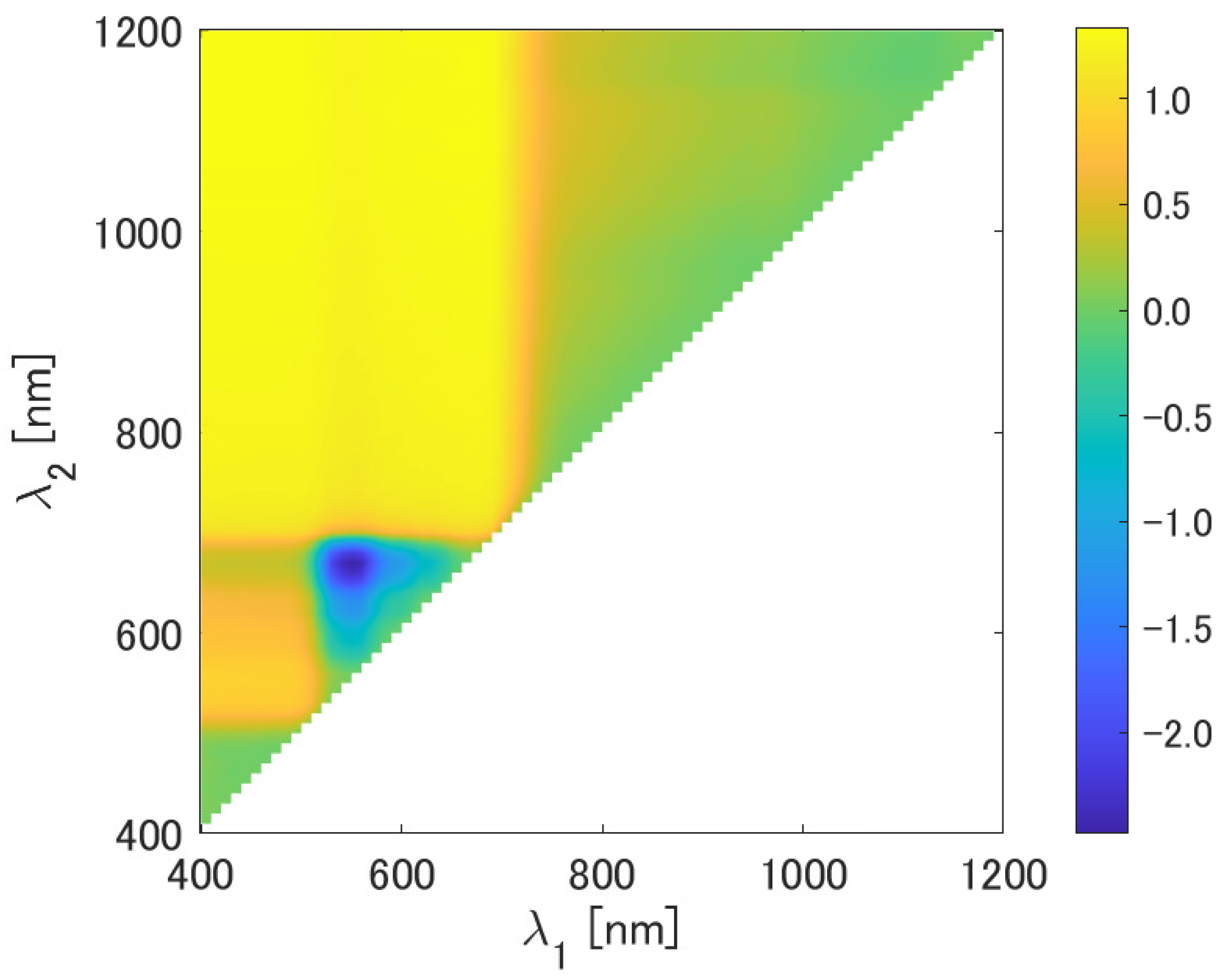
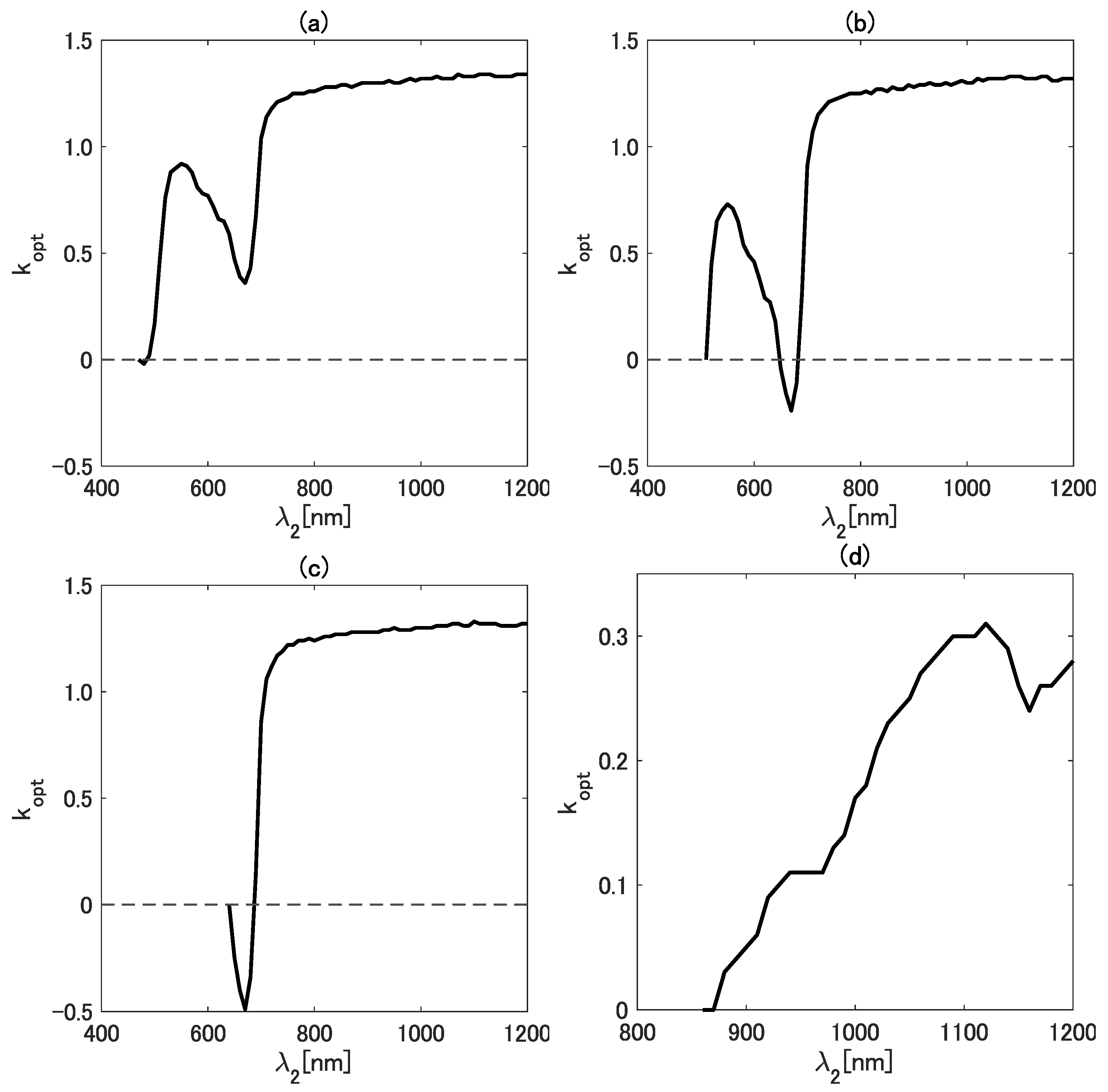
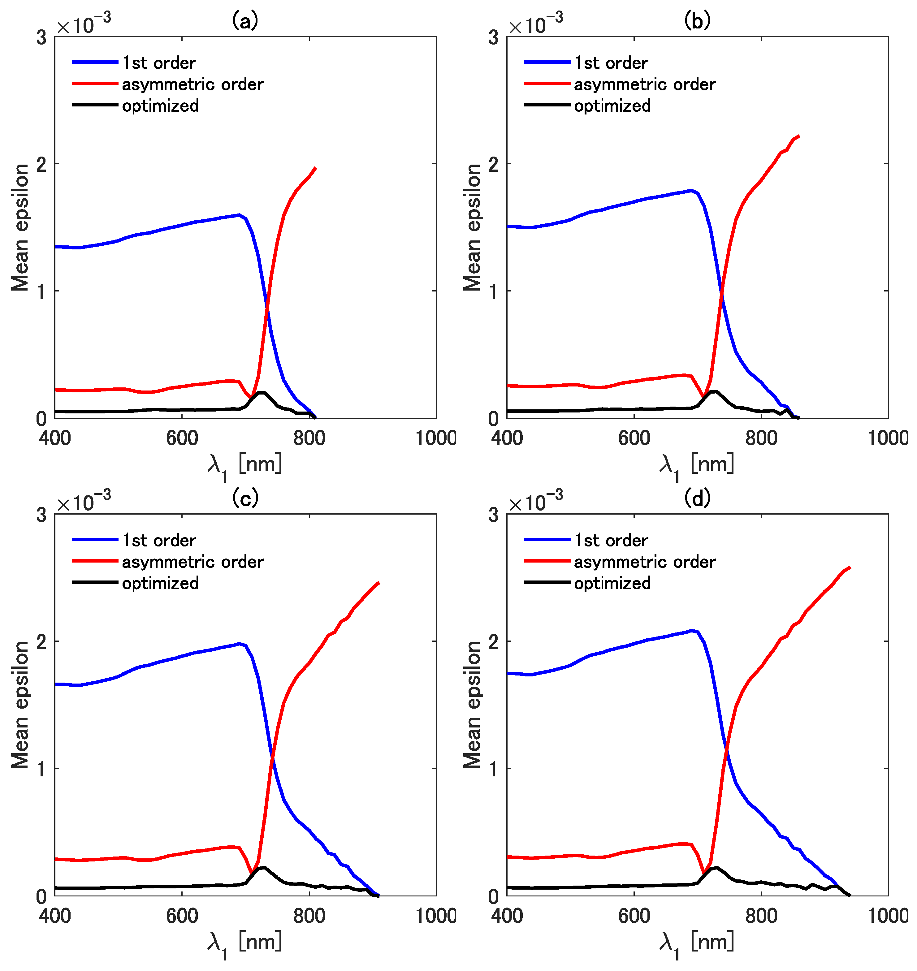
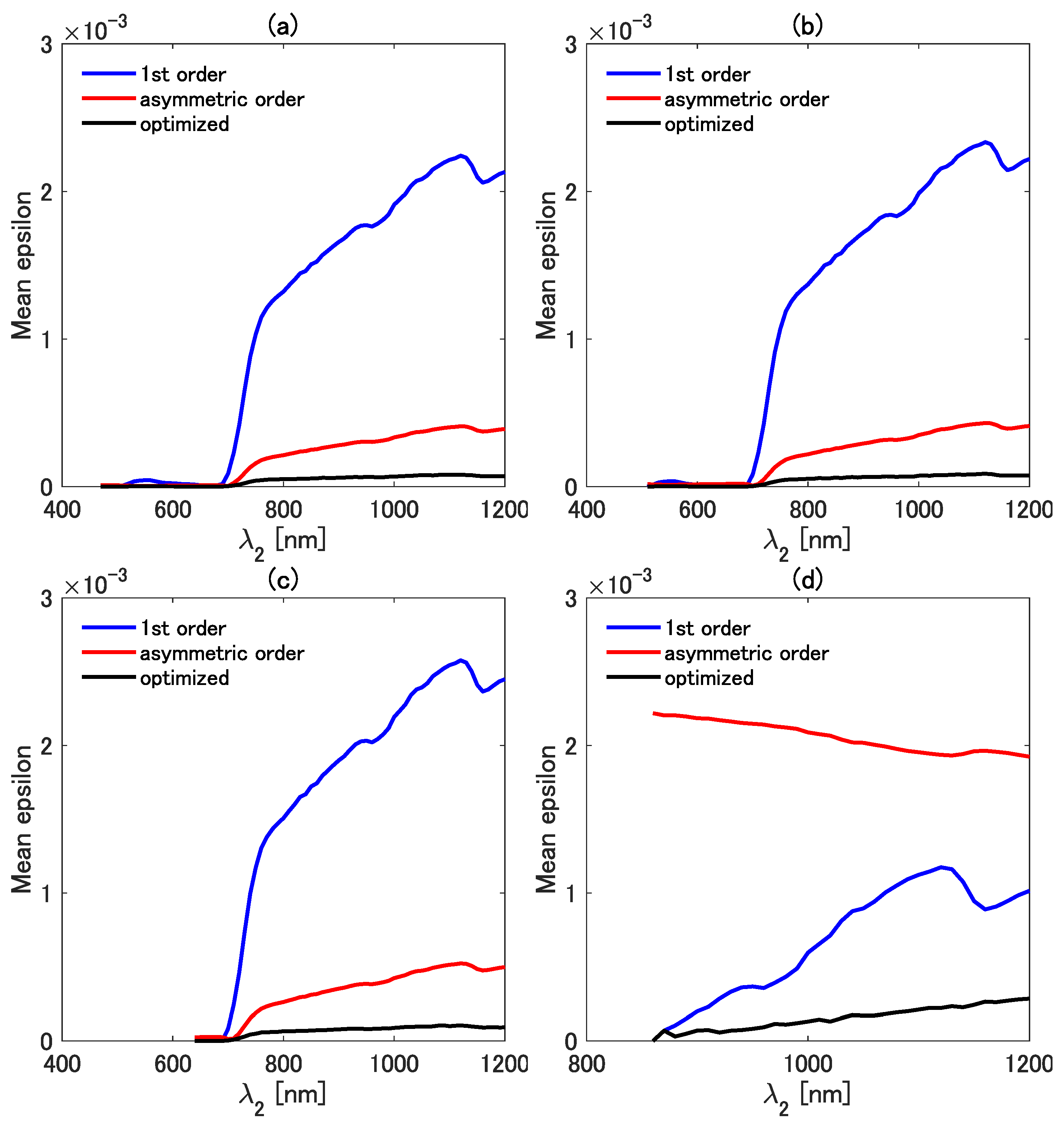
4.1. Analysis of
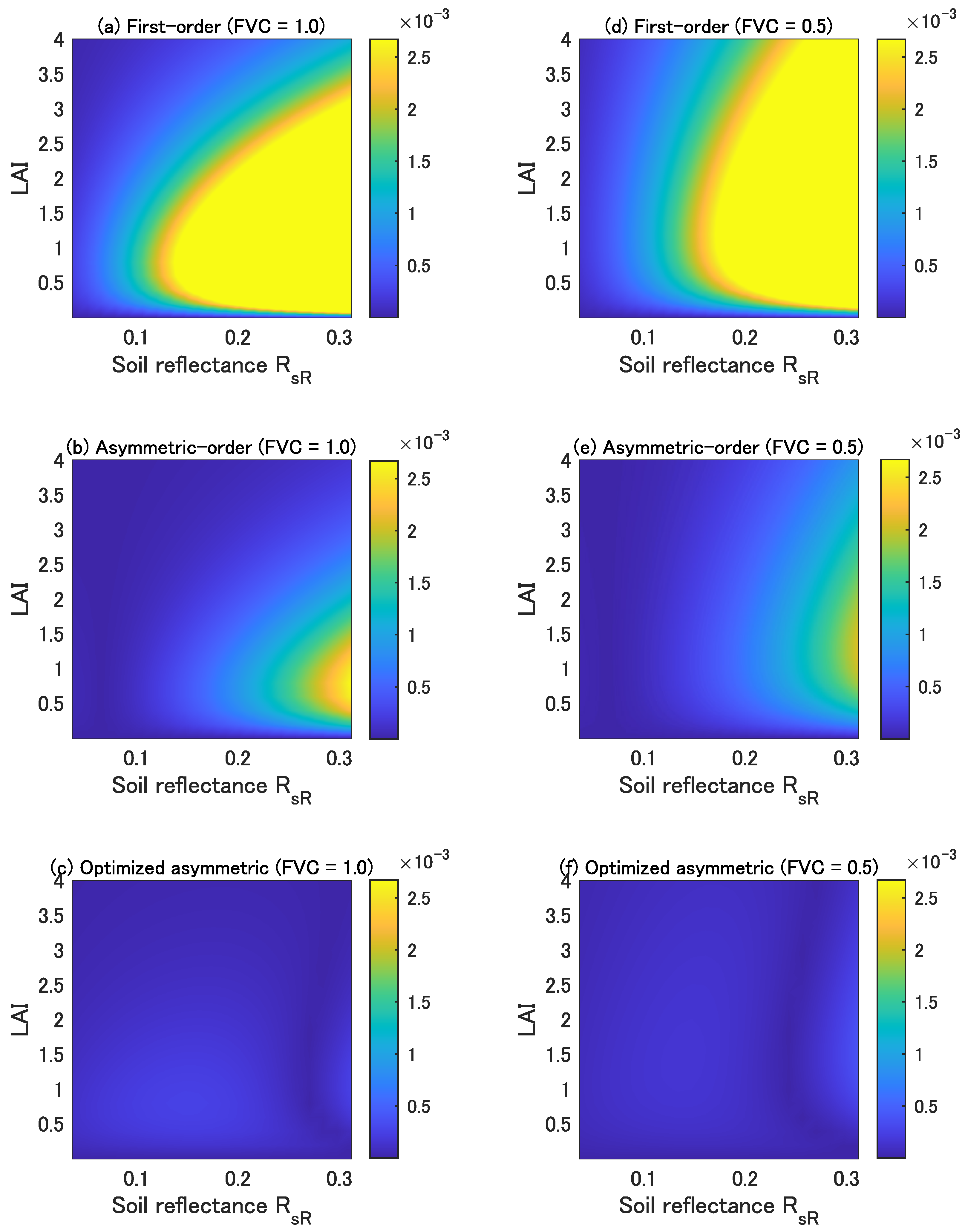
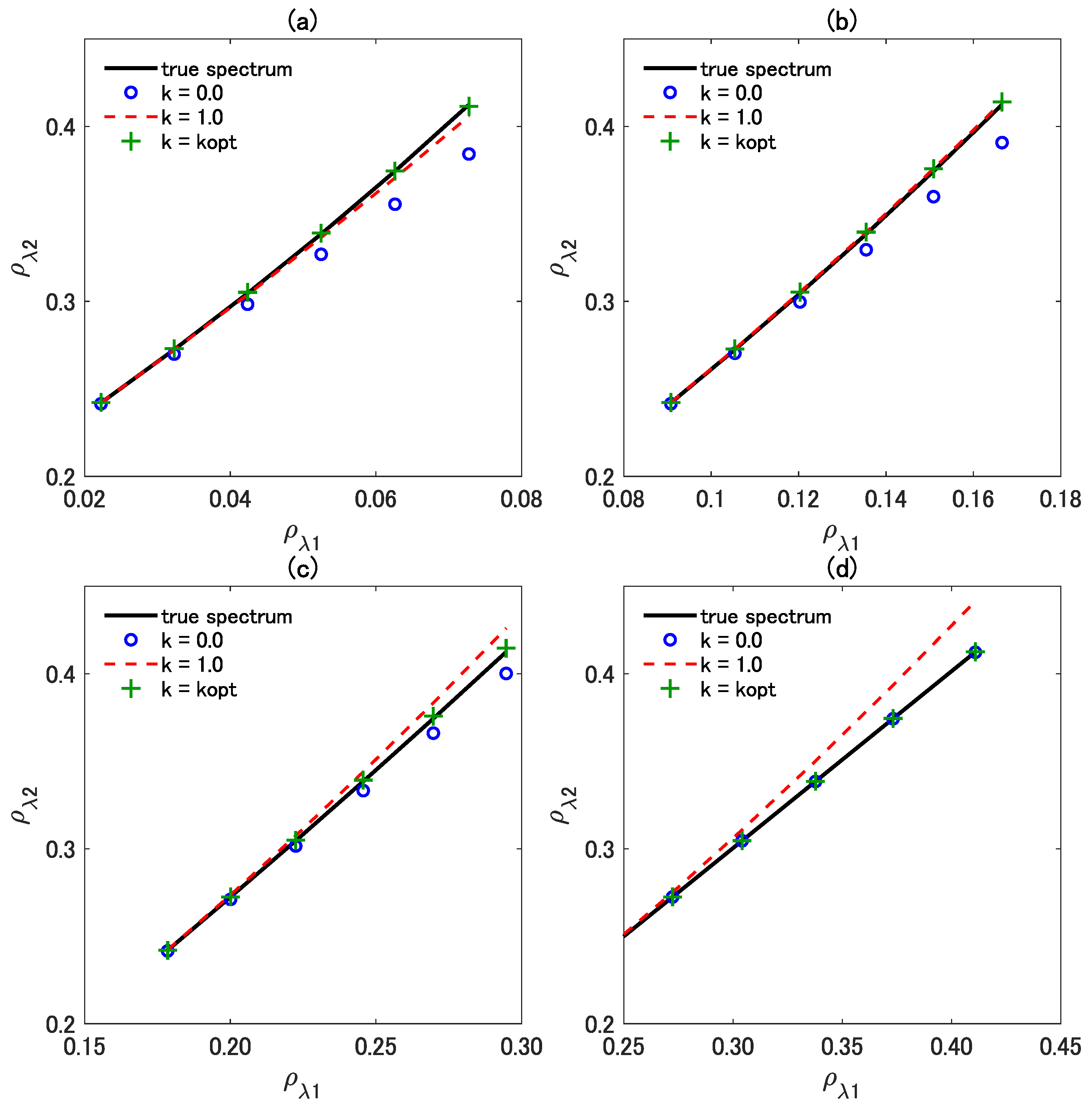
4.2. Accuracy of the Three Vegetation Isolines
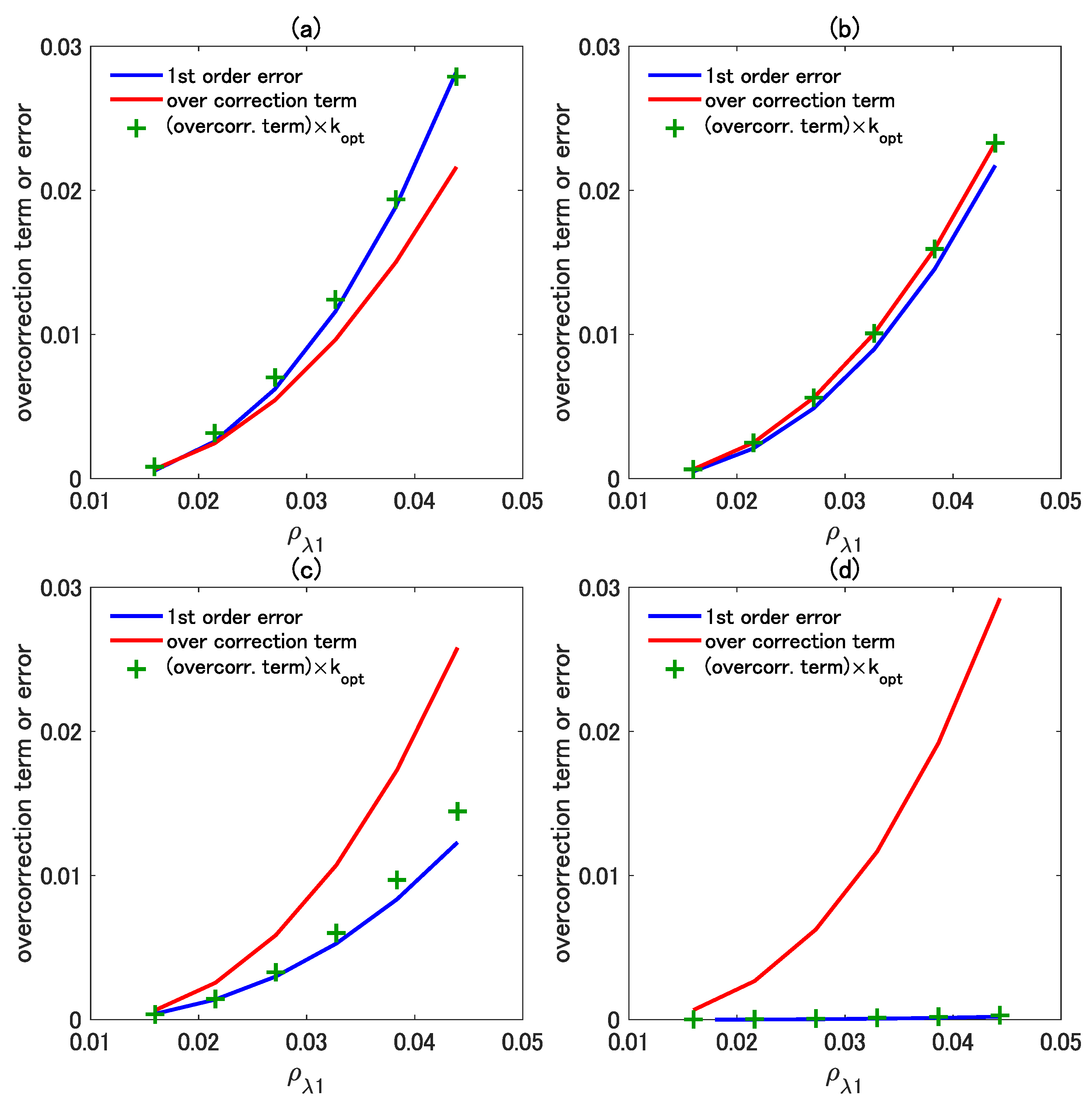
4.3. Influence of the Higher-Order Interaction Terms Demonstrated in the Reflectance Subspace
5. Discussion
6. Conclusions
Author Contributions
Funding
Data Availability Statement
Conflicts of Interest
References
- Zhu, Z.; Bi, J.; Pan, Y.; Ganguly, S.; Anav, A.; Xu, L.; Samanta, A.; Piao, S.; Nemani, R.R.; Myneni, R.B. Global data sets of vegetation leaf area index (LAI) 3g and fraction of photosynthetically active radiation (FPAR) 3g derived from global inventory modeling and mapping studies (GIMMS) normalized difference vegetation index (NDVI3g) for the period 1981 to 2011. Remote Sens. 2013, 5, 927–948. [Google Scholar] [CrossRef] [Green Version]
- Hansen, M.C.; Potapov, P.V.; Moore, R.; Hancher, M.; Turubanova, S.A.; Tyukavina, A.; Thau, D.; Stehman, S.; Goetz, S.J.; Loveland, T.R.; et al. High-resolution global maps of 21st-century forest cover change. Science 2013, 342, 850–853. [Google Scholar] [CrossRef] [PubMed] [Green Version]
- Huete, A.R. A soil-adjusted vegetation index (SAVI). Remote Sens. Environ. 1988, 25, 295–309. [Google Scholar] [CrossRef]
- Baret, F.; Guyot, G.; Major, D. TSAVI: A vegetation index which minimizes soil brightness effects on LAI and APAR estimation. In Proceedings of the 12th Canadian Symposium on Remote Sensing Geoscience and Remote Sensing Symposium, Vancouver, BC, Canada, 10–14 July 1989; Volume 3, pp. 1355–1358. [Google Scholar] [CrossRef]
- Major, D.; Baret, F.; Guyot, G. A ratio vegetation index adjusted for soil brightness. Int. J. Remote Sens. 1990, 11, 727–740. [Google Scholar] [CrossRef]
- Qi, J.; Chehbouni, A.; Huete, A.; Kerr, Y.; Sorooshian, S. A modified soil adjusted vegetation index. Remote Sens. Environ. 1994, 48, 119–126. [Google Scholar] [CrossRef]
- Verstraete, M.M.; Pinty, B. Designing optimal spectral indexes for remote sensing applications. IEEE Trans. Geosci. Remote Sens. 1996, 34, 1254–1265. [Google Scholar] [CrossRef]
- Gilabert, M.; González-Piqueras, J.; Garcıa-Haro, F.; Meliá, J. A generalized soil-adjusted vegetation index. Remote Sens. Environ. 2002, 82, 303–310. [Google Scholar] [CrossRef]
- Jiang, Z.; Huete, A.R.; Didan, K.; Miura, T. Development of a two-band enhanced vegetation index without a blue band. Remote Sens. Environ. 2008, 112, 3833–3845. [Google Scholar] [CrossRef]
- Yoshioka, H.; Huete, A.R.; Miura, T. Derivation of vegetation isoline equations in red-NIR reflectance space. IEEE Trans. Geosci. Remote Sens. 2000, 38, 838–848. [Google Scholar] [CrossRef]
- Yoshioka, H.; Miura, T.; Huete, A.; Ganapol, B.D. Analysis of vegetation isolines in red-NIR reflectance space. Remote Sens. Environ. 2000, 74, 313–326. [Google Scholar] [CrossRef]
- Yoshioka, H. Vegetation isoline equations for an atmosphere-canopy-soil system. IEEE Trans. Geosci. Remote Sens. 2004, 42, 166–175. [Google Scholar] [CrossRef]
- Miura, M.; Obata, K.; Yoshioka, H. Vegetation isoline equations with first-and second-order interaction terms for modeling a canopy-soil system of layers in the red and near-infrared reflectance space. J. App. Remote Sens. 2015, 9, 095987. [Google Scholar] [CrossRef] [Green Version]
- Miura, M.; Obata, K.; Taniguchi, K.; Yoshioka, H. Improved accuracy of the asymmetric second-order vegetation isoline equation over the red–NIR reflectance space. Sensors 2017, 17, 450. [Google Scholar] [CrossRef] [PubMed] [Green Version]
- Miura, M.; Obata, K.; Taniguchi, K.; Yoshioka, H. Optimization technique of asymmetric-order vegetation isoline equations. In Proceedings of the 2017 IEEE International Geoscience and Remote Sensing Symposium (IGARSS), Fort Worth, TX, USA, 23–28 July 2017; pp. 2923–2926. [Google Scholar] [CrossRef]
- Yoshioka, H.; Miura, T.; Demattê, J.A.; Batchily, K.; Huete, A.R. Derivation of soil line influence on two-band vegetation indices and vegetation isolines. Remote Sens. 2009, 1, 842–857. [Google Scholar] [CrossRef] [Green Version]
- Yoshioka, H.; Miura, T.; Demattê, J.A.; Batchily, K.; Huete, A.R. Soil line influences on two-band vegetation indices and vegetation isolines: A numerical study. Remote Sens. 2010, 2, 545–561. [Google Scholar] [CrossRef] [Green Version]
- Fan, X.; Liu, Y. Multisensor Normalized Difference Vegetation Index Intercalibration: A comprehensive overview of the causes of and solutions for multisensor differences. IEEE Geosci. Remote Sens. Mag. 2018, 6, 23–45. [Google Scholar] [CrossRef]
- Sun, Y.; Lu, L.; Liu, Y. Inversion of the leaf area index of rice fields using vegetation isoline patterns considering the fraction of vegetation cover. Int. J. Remote Sens. 2021, 42, 1688–1712. [Google Scholar] [CrossRef]
- Baret, F.; Guyot, G. Potentials and limits of vegetation indices for LAI and APAR assessment. Remote Sens. Environ. 1991, 35, 161–173. [Google Scholar] [CrossRef]
- Jackson, R.; Pinter, P., Jr.; Reginato, R.; Idso, S. Hand-Held Radiometry: A Set of Notes Developed for Use at the Workshop of Hand-Held Radiometry; Technical Report; Agricultural Research (Western Region), Science and Education Administration, U.S. Department of Agriculture: Phoenix, AZ, USA, 1980.
- Kimes, D.S.; Norman, J.M.; Walthall, C.L. Modeling the radiant transfers of sparse vegetation canopies. IEEE Trans. Geosci. Remote Sens. 1985, GE-23, 695–704. [Google Scholar] [CrossRef]
- Sellers, P.J. Canopy reflectance, photosynthesis and transpiration. Int. J. Remote Sens. 1985, 6, 1335–1372. [Google Scholar] [CrossRef]
- Huete, A.; Jackson, R. Suitability of spectral indices for evaluating vegetation characteristics on arid rangelands. Remote Sens. Environ. 1987, 23, 213–232, IN1–IN8. [Google Scholar] [CrossRef]
- Gobron, N.; Pinty, B.; Verstraete, M.M.; Widlowski, J.L. Advanced vegetation indices optimized for up-coming sensors: Design, performance, and applications. IEEE Trans. Geosci. Remote. Sens. 2000, 38, 2489–2505. [Google Scholar] [CrossRef]
- Yoshioka, H.; Yamamoto, H.; Miura, T. Use of an isoline-based inversion technique to retrieve a leaf area index for inter-sensor calibration of spectral vegetation index. In Proceedings of the IEEE International Geoscience and Remote Sensing Symposium, IGARSS’02, Toronto, ON, Canada, 24–28 June 2002; Volume 3, pp. 1639–1641. [Google Scholar] [CrossRef]
- Kallel, A.; Le Hégarat-Mascle, S.; Ottlé, C.; Hubert-Moy, L. Determination of vegetation cover fraction by inversion of a four-parameter model based on isoline parametrization. Remote Sens. Environ. 2007, 111, 553–566. [Google Scholar] [CrossRef]
- Okuda, K.; Taniguchi, K.; Miura, M.; Obata, K.; Yoshioka, H. Application of vegetation isoline equations for simultaneous retrieval of leaf area index and leaf chlorophyll content using reflectance of red edge band. In Remote Sensing and Modeling of Ecosystems for Sustainability XIII; International Society for Optics and Photonics: Bellingham, WA, USA, 2016; Volume 9975, p. 99750C. [Google Scholar] [CrossRef]
- Yoshioka, H.; Miura, T.; Huete, A.R. An isoline-based translation technique of spectral vegetation index using EO-1 Hyperion data. IEEE Trans. Geosci. Remote Sens. 2003, 41, 1363–1372. [Google Scholar] [CrossRef]
- Yoshioka, H.; Miura, T.; Yamamoto, H. Analytical relationships of inter-sensor vegetation indices based on the theory of vegetation isoline. In Proceedings of the IEEE International Geoscience and Remote Sensing Symposium, IGARSS’05, Seoul, Korea, 29 July 2005; Volume 6, pp. 4164–4167. [Google Scholar] [CrossRef]
- Yoshioka, H.; Miura, T.; Obata, K. Derivation of relationships between spectral vegetation indices from multiple sensors based on vegetation isolines. Remote Sens. 2012, 4, 583–597. [Google Scholar] [CrossRef] [Green Version]
- Obata, K.; Miura, T.; Yoshioka, H.; Huete, A.R. Derivation of a MODIS-compatible enhanced vegetation index from visible infrared imaging radiometer suite spectral reflectances using vegetation isoline equations. J. App. Remote Sens. 2013, 7, 073467. [Google Scholar] [CrossRef] [Green Version]
- Fan, X.; Liu, Y. A generalized model for intersensor NDVI calibration and its comparison with regression approaches. IEEE Trans. Geosci. Remote Sens. 2016, 55, 1842–1852. [Google Scholar] [CrossRef]
- Iwasaki, A.; Ohgi, N.; Tanii, J.; Kawashima, T.; Inada, H. Hyperspectral Imager Suite (HISUI)-Japanese hyper-multi spectral radiometer. In Proceedings of the 2011 IEEE International Geoscience and Remote Sensing Symposium, Vancouver, BC, Canada, 24–29 July 2011; pp. 1025–1028. [Google Scholar] [CrossRef]
- Obata, K.; Tsuchida, S.; Nagatani, I.; Yamamoto, H.; Kouyama, T.; Yamada, Y.; Yamaguchi, Y.; Ishii, J. An overview of ISS HISUI hyperspectral imager radiometric calibration. In Proceedings of the 2016 IEEE International Geoscience and Remote Sensing Symposium (IGARSS), Beijing, China, 10–15 July 2016; pp. 1924–1927. [Google Scholar] [CrossRef]
- Matsunaga, T.; Iwasaki, A.; Tsuchida, S.; Iwao, K.; Nakamura, R.; Yamamoto, H.; Kato, S.; Obata, K.; Kashimura, O.; Tanii, J.; et al. HISUI status toward FY2019 launch. In Proceedings of the IGARSS 2018-2018 IEEE International Geoscience and Remote Sensing Symposium, Valencia, Spain, 22–27 July 2018; pp. 160–163. [Google Scholar] [CrossRef]
- Obata, K. Sensitivity analysis method for spectral band adjustment between hyperspectral sensors: A case study using the CLARREO Pathfinder and HISUI. Remote Sens. 2019, 11, 1367. [Google Scholar] [CrossRef] [Green Version]
- Guanter, L.; Kaufmann, H.; Segl, K.; Foerster, S.; Rogass, C.; Chabrillat, S.; Kuester, T.; Hollstein, A.; Rossner, G.; Chlebek, C.; et al. The EnMAP Spaceborne Imaging Spectroscopy Mission for Earth Observation. Remote Sens. 2015, 7, 8830–8857. [Google Scholar] [CrossRef] [Green Version]
- Alonso, K.; Bachmann, M.; Burch, K.; Carmona, E.; Cerra, D.; de los Reyes, R.; Dietrich, D.; Heiden, U.; Hölderlin, A.; Ickes, J.; et al. Data Products, Quality and Validation of the DLR Earth Sensing Imaging Spectrometer (DESIS). Sensors 2019, 19, 4471. [Google Scholar] [CrossRef] [Green Version]
- Vangi, E.; D’Amico, G.; Francini, S.; Giannetti, F.; Lasserre, B.; Marchetti, M.; Chirici, G. The New Hyperspectral Satellite PRISMA: Imagery for Forest Types Discrimination. Sensors 2021, 21, 1182. [Google Scholar] [CrossRef] [PubMed]
- Baret, F.; Jacquemoud, S.; Hanocq, J. The soil line concept in remote sensing. Remote Sens. Rev. 1993, 7, 65–82. [Google Scholar] [CrossRef]
- Obata, K.; Taniguchi, K.; Matsuoka, M.; Yoshioka, H. Development and Demonstration of a Method for GEO-to-LEO NDVI Transformation. Remote Sens. 2021, 13, 4085. [Google Scholar] [CrossRef]
- Jacquemoud, S.; Verhoef, W.; Baret, F.; Bacour, C.; Zarco-Tejada, P.J.; Asner, G.P.; François, C.; Ustin, S.L. PROSPECT+ SAIL models: A review of use for vegetation characterization. Remote Sens. Environ. 2009, 113, S56–S66. [Google Scholar] [CrossRef]
- Jacquemoud, S.; Baret, F. PROSPECT: A model of leaf optical properties spectra. Remote Sens. Environ. 1990, 34, 75–91. [Google Scholar] [CrossRef]
- Verhoef, W. Light scattering by leaf layers with application to canopy reflectance modeling: The SAIL model. Remote Sens. Environ. 1984, 16, 125–141. [Google Scholar] [CrossRef] [Green Version]
- Bessho, K.; Date, K.; Hayashi, M.; Ikeda, A.; Imai, T.; Inoue, H.; Kumagai, Y.; Miyakawa, T.; Murata, H.; Ohno, T.; et al. An introduction to Himawari-8/9—Japan’s new-generation geostationary meteorological satellites. J. Meteorol. Soc. Japan. Ser. II 2016, 94, 151–183. [Google Scholar] [CrossRef] [Green Version]
- Adachi, Y.; Kikuchi, R.; Matsuoka, M.; Ichii, K.; Yoshioka, H. Reflectance comparison between Himawari-8 AHI and Terra MODIS over a forest of Shikoku region. In Land Surface and Cryosphere Remote Sensing IV; International Society for Optics and Photonics: Bellingham, WA, USA, 2018; Volume 10777, p. 1077715. [Google Scholar] [CrossRef]
- Miura, T.; Nagai, S.; Takeuchi, M.; Ichii, K.; Yoshioka, H. Improved characterisation of vegetation and land surface seasonal dynamics in central Japan with Himawari-8 hypertemporal data. Sci. Rep. 2019, 9, 15692. [Google Scholar] [CrossRef] [Green Version]
- Wang, W.; Li, S.; Hashimoto, H.; Takenaka, H.; Higuchi, A.; Kalluri, S.; Nemani, R. An introduction to the Geostationary-NASA Earth Exchange (GeoNEX) Products: 1. Top-of-atmosphere reflectance and brightness temperature. Remote Sens. 2020, 12, 1267. [Google Scholar] [CrossRef] [Green Version]
- Obata, K.; Yoshioka, H. A Simple Algorithm for Deriving an NDVI-Based Index Compatible between GEO and LEO Sensors: Capabilities and Limitations in Japan. Remote Sens. 2020, 12, 2417. [Google Scholar] [CrossRef]
- Xiao, J.; Fisher, J.B.; Hashimoto, H.; Ichii, K.; Parazoo, N.C. Emerging satellite observations for diurnal cycling of ecosystem processes. Nat. Plants 2021, 7, 877–887. [Google Scholar] [CrossRef] [PubMed]
- Hashimoto, H.; Wang, W.; Dungan, J.L.; Li, S.; Michaelis, A.R.; Takenaka, H.; Higuchi, A.; Myneni, R.B.; Nemani, R.R. New generation geostationary satellite observations support seasonality in greenness of the Amazon evergreen forests. Nat. Commun. 2021, 12, 684. [Google Scholar] [CrossRef] [PubMed]
- Zhao, H.S.; Zhu, X.C.; Li, C.; Wei, Y.; Zhao, G.X.; Jiang, Y.M. Improving the accuracy of the hyperspectral model for apple canopy water content prediction using the equidistant sampling method. Sci. Rep. 2017, 7, 11192. [Google Scholar] [CrossRef] [PubMed] [Green Version]
- Ali, A.M.; Darvishzadeh, R.; Skidmore, A.; Heurich, M.; Paganini, M.; Heiden, U.; Mücher, S. Evaluating prediction models for mapping canopy chlorophyll content across biomes. Remote Sens. 2020, 12, 1788. [Google Scholar] [CrossRef]
- Ali, A.M.; Darvishzadeh, R.; Skidmore, A.; Gara, T.W.; O’ Connor, B.; Roeoesli, C.; Heurich, M.; Paganini, M. Comparing methods for mapping canopy chlorophyll content in a mixed mountain forest using Sentinel-2 data. Int. J. Appl. Earth Obs. Geoinf. 2020, 87, 102037. [Google Scholar] [CrossRef]
- Folkman, M.A.; Pearlman, J.; Liao, L.B.; Jarecke, P.J. EO-1/Hyperion hyperspectral imager design, development, characterization, and calibration. In Hyperspectral Remote Sensing of the Land and Atmosphere; Smith, W.L., Yasuoka, Y., Eds.; International Society for Optics and Photonics, SPIE: Bellingham, WA, USA, 2001; Volume 4151, pp. 40–51. [Google Scholar] [CrossRef]
- Donohue, R.J.; Roderick, M.L.; McVicar, T.R. Deriving consistent long-term vegetation information from AVHRR reflectance data using a cover-triangle-based framework. Remote Sens. Environ. 2008, 112, 2938–2949. [Google Scholar] [CrossRef]
- Zhang, X.; Tan, B.; Yu, Y. Interannual variations and trends in global land surface phenology derived from enhanced vegetation index during 1982–2010. Int. J. Biometeorol. 2014, 58, 547–564. [Google Scholar] [CrossRef] [Green Version]
- Fan, X.; Liu, Y. A comparison of NDVI intercalibration methods. Int. J. Remote Sens. 2017, 38, 5273–5290. [Google Scholar] [CrossRef]


| Geometry | |
| Solar zenith angle | 30 |
| Observation zenith angle | 10 |
| Relative azimuth angle | 0 |
| Pixel heterogeneous property | |
| Fraction of vegetation cover (FVC) | 0.0–1.0 |
| Canopy properties | |
| Leaf area index (LAI) | 0.0–4.0 |
| Hotspot size parameter | 0.01 |
| Leaf structural and chemical properties | |
| Leaf angle distribution (LAD) | Spherical |
| Leaf mesophyll structure | 1.5 |
| Chlorophyll-a and -b | 40 g/cm |
| Carotenoid content | 8 g/cm |
| Leaf mass per area | 0.009 g/cm |
| Equivalent water thickness | 0.01 cm |
| Brown pigment content | 0 |
| Soil properties | |
| Soil factor (mixture ratio of wet and dry soils) | 0.0–1.0 [0.0: wet soil; 1.0: dry soil] |
| Spectral bands | |
| Wavelength | 410 nm to 1200 nm |
| Wavelength | 400 nm to nm |
Publisher’s Note: MDPI stays neutral with regard to jurisdictional claims in published maps and institutional affiliations. |
© 2022 by the authors. Licensee MDPI, Basel, Switzerland. This article is an open access article distributed under the terms and conditions of the Creative Commons Attribution (CC BY) license (https://creativecommons.org/licenses/by/4.0/).
Share and Cite
Miura, M.; Obata, K.; Yoshioka, H. Wavelength Extension of the Optimized Asymmetric-Order Vegetation Isoline Equation to Cover the Range from Visible to Near-Infrared. Remote Sens. 2022, 14, 2289. https://0-doi-org.brum.beds.ac.uk/10.3390/rs14092289
Miura M, Obata K, Yoshioka H. Wavelength Extension of the Optimized Asymmetric-Order Vegetation Isoline Equation to Cover the Range from Visible to Near-Infrared. Remote Sensing. 2022; 14(9):2289. https://0-doi-org.brum.beds.ac.uk/10.3390/rs14092289
Chicago/Turabian StyleMiura, Munenori, Kenta Obata, and Hiroki Yoshioka. 2022. "Wavelength Extension of the Optimized Asymmetric-Order Vegetation Isoline Equation to Cover the Range from Visible to Near-Infrared" Remote Sensing 14, no. 9: 2289. https://0-doi-org.brum.beds.ac.uk/10.3390/rs14092289