Article

Comparison of Different Important Predictors and Models for Estimating Large-Scale Biomass of Rubber Plantations in Hainan Island, China

1
Co-Innovation Center for Sustainable Forestry in Southern China, Nanjing Forestry University, Nanjing 210037, China
2
Rubber Research Institute (RRI), Chinese Academy of Tropical Agricultural Sciences (CATAS), Hainan Danzhou Agro-Ecosystem National Observation and Research Station, State Key Laboratory Incubation Base for Cultivation & Physiology of Tropical Crops, Haikou 571101, China
*
Author to whom correspondence should be addressed.
Remote Sens. 2023, 15(13), 3447; https://0-doi-org.brum.beds.ac.uk/10.3390/rs15133447
Submission received: 5 May 2023 / Revised: 26 June 2023 / Accepted: 5 July 2023 / Published: 7 July 2023
(This article belongs to the Special Issue Forest Biomass/Carbon Monitoring towards Carbon Neutrality)

Abstract

:
Rubber (Hevea brasiliensis Muell.) plantations are among the most critical agricultural ecosystems in tropical regions, playing a vital role in regional carbon balance. Accurate large-scale biomass estimation for these plantations remains a challenging task due to the severe signal saturation problem. Recent advances in remote sensing big data, cloud platforms, and machine learning have facilitated the precise acquisition of key physiological variables, such as stand age (A) and canopy height (H), which are critical parameters for biomass estimation but have been underutilized in prior studies. Using Hainan Island—the second-largest rubber planting base in China—as a case study, we integrated extensive ground surveys, maps of stand age and canopy height, remote sensing indicators (RSIs), and geographical and climate indicators (ECIs) to ascertain the optimal method for estimating rubber plantation biomass. We compared different inputs and estimation approaches (direct and indirect) using the random forest algorithm and analyzed the spatiotemporal characteristics of rubber plantation biomass on Hainan Island. The results indicated that the traditional model (RSIs + ECIs) had low accuracy and significant estimation bias (R2 = 0.24, RMSE = 38.36 mg/ha). The addition of either stand age or canopy height considerably enhance model accuracy (R2 = 0.77, RMSE ≈ 21.12 mg/ha). Moreover, incorporating the DBH obtained through indirect inversion yielded even greater predictive accuracy (R2 = 0.97, RMSE = 7.73 mg/ha), outperforming estimates derived from an allometric equation model input with the DBH (R2 = 0.67, RMSE = 25.43 mg/ha). However, augmenting the model with stand age, canopy height, or their combination based on RSIs, ECIs, and DBH only marginally improved the accuracy. Consequently, it is not recommended in scenarios with limited data and computing resources. Employing the optimal model, we generated biomass maps of rubber plantations on Hainan Island for 2016 and 2020, revealing that the spatiotemporal distribution pattern of the biomass is closely associated with the establishment year of the rubber plantations. While average biomass in a few areas has undergone slight decreases, total biomass has exhibited significant growth, reaching 5.46 × 10⁷ mg by the end of 2020, underscoring its considerable value as a carbon sink.

1. Introduction

Biomass, defined as the accumulation of dry matter per unit time or area, represents a fundamental quantitative attribute of forest ecosystems [1,2,3]. Fluctuations in biomass mirror alterations and influences stemming from forest, climate, and human activities, rendering it an essential parameter for assessing vegetation carbon stocks and examining shifts in forest ecosystem structure and function [4,5,6]. Consequently, the accurate description and estimation of biomass are vital to a wide array of scientific endeavors [7]. In light of societal advancement, resource utilization, and global climate change, the investigation of biomass and carbon stocks has undergone significant expansion, with related research consistently receiving substantial interest [8].
Numerous methods exist for estimating biomass, with the precision and spatial scale of these approaches varying significantly [9]. Traditional field measurement remains the most accurate estimation technique, and the established allometric equation (AE) often serves as a critical foundation for alternative methods [2,5]. However, this approach is both time-consuming and spatially constrained [5]. Owing to its high spatial, temporal, and spectral resolution, as well as its capacity for continuous, long-term scientific observations, remote sensing technology has become a widely employed tool for biomass estimation [10,11,12,13]. Broadly speaking, forest biomass estimation via remote sensing has evolved through three stages: (1) estimation solely based on optical, radar, or Light Detection and Ranging (LiDAR) data [14,15]; (2) effective incorporation of multiple types of satellite imagery, mitigating the limitations of solitary satellite imagery data [16]; (3) selection of optimal variables from multi-source satellite imagery and ancillary data [5], thereby enhancing model accuracy [12,17].
Rubber (Hevea brasiliensis Muell.), a tall tree native to the Amazon basin, constitutes the primary source of natural rubber [3,6,18]. In response to the burgeoning industrial and economic growth, the tree has been extensively cultivated in Southeast Asia and the tropical regions of China since the last century [3]. Prompted by the swift escalation of natural rubber prices in the 2000s, global rubber plantation coverage has undergone rapid expansion, rendering rubber plantations significant ecosystems within numerous tropical regions. Beyond providing natural rubber, rubber plantations fulfill the ecological roles commonly associated with typical forests, such as carbon sequestration [19,20]. Studies indicate that total carbon stocks within rubber plantations surpass those of many tropical forests and agroforestry ecosystems, contributing positively to climate change mitigation efforts [21]. Accurate estimates of rubber plantation biomass are essential for predicting natural rubber yield [22], analyzing intrinsic dynamics, and understanding the carbon cycle in the tropics [21,23].
Numerous studies have investigated biomass estimation in rubber plantations; however, the primary study areas have been concentrated on Hainan Island and in Xishuangbanna, China [24,25,26,27,28]. Methodological evolution has advanced from initial direct remote sensing inversion to the incorporation of vital physiological parameters, such as stand age [14,19,23]. Rubber plantations are typically established concurrently, resulting in uniform stand age, which correlates closely with biomass and can be estimated using dense time-series satellite imagery [20]. For example, the authors of [6] combined stand age with the random forest algorithm to estimate the biomass of rubber plantations in Hainan Island, achieving an R2 of 0.82 to 0.96 and root-mean-square error (RMSE) of 4.08 to 10.59 mg/ha. However, stand age is not the most ideal parameter for biomass estimation, as rubber tree growth conditions vary across different geographical environments despite identical ages. Diameter at breast height (DBH) is the simplest parameter to measure for plantations, but its large-scale measurement and accurate remote sensing retrieval pose challenges. Fortunately, the recently launched Global Ecosystem Dynamics Investigation (GEDI) satellite can accurately obtain high-resolution forest canopy heights on a global scale, which can be utilized for precise forest biomass estimation [29]. For example, Nico et al. (2022) fused GEDI and Landsat images to obtain a global canopy height product with a resolution of 10 m for 2020 [30]; Sun et al. (2022) found high accuracy in aboveground biomass (AGB) estimation using GEDI canopy metrics (R2 = 0.82, RMSE = 19.1 mg/ha) [31]. Consequently, we hypothesize that integrating stand age, canopy height, remote sensing indices (RSIs), and environment and climate indices (ECIs) may yield a more accurate rubber plantation biomass estimation. The specific aim of this study was to employ machine learning algorithms to compare the effects of different variable combinations (stand age, canopy height, RSIs, and ECIs) and estimation methodologies (direct and indirect estimates) on the accuracy of rubber plantation biomass estimation.

2. Materials and Methods

2.1. Study Area

Hainan Island, with a total area of approximately 3.4 million hectares, possesses a topography typified by peripheral lowlands and a central mountainous prominence. The region is subject to a tropical monsoon maritime climate, exhibiting annual mean temperatures between 23 °C and 25 °C. The island’s iso-precipitation line distribution indicates elevated concentrations in the central and eastern areas, whereas diminished concentrations are observed along the southwestern coast. Furthermore, Hainan Island is characterized by pronounced rainy and dry seasons, with the former extending from May to October and constituting approximately 80% of the overall annual precipitation.
Since the 1950s, extensive rubber plantations have been established on Hainan Island to promote economic, scientific, and technological advancements [27]. Hainan Island, once the largest rubber plantation area in China, has been surpassed by Yunnan province, and it now ranks second with an approximate area of 520,000 hectares. Rubber plantations on Hainan Island are predominantly located in the northwest, central, and northern regions, accounting for over 25% of the total forest area and forming the largest plantation ecosystem on the island [32,33].

2.2. Data and Processing

2.2.1. Field Inventory Data

Field data were procured from sampled plots across the island and long-term positioning monitoring plots located at the experimental farm of the Chinese Academy of Tropical Agricultural Sciences (CATAS). The field investigation took place in October 2016, during which time 70 rubber plantations with diverse stand ages on Hainan Island were selected for analysis. For each rubber tree within a 25 × 25 m zone in each plantation, DBH using a 1.3 m height was measured. Rubber stand age was determined through both field estimation and an algorithm analyzing time-series satellite imagery dating back to 1987 [34]. To correspond with the canopy height map in 2020 (elaborated in Section 2.2.3), these samples were further scrutinized using Google Earth high-resolution imagery, retaining only the sample plots with accurate geolocation and persistence in 2020. In a prior biomass estimation study, a mere 51 samples with precise geolocations and stand ages under 30 years were utilized [6]. Due to advancements in stand age monitoring technology employing satellite images, 58 samples remained accessible after excluding the rubber plantations harvested in 2020 (Figure 1). Among these samples, only a few overlapped with the GEDI footprint in 2020.
At the CATAS experimental farm, there are nine long-term positioning monitoring plots ranging from 1.39 to 2.98 hectares. From 2007 to 2014, the DBH of each tree was measured monthly during the seedling stage (≤4 years) and subsequently at quarterly or semi-annual intervals as trees grew taller. The DBH for the rubber plantations from 2007 to 2014 was calculated using Equation (1):
D g = i = 1 N d i 2 N
where D g is the mean DBH, d i is the DBH of the i t h tree in the stand, and N is the total number of trees. The total biomass of each plantation ( B A E , mg/ha) was calculated using Equation (2), which was developed based on an AE model, taking into account initial planting density and tree loss due to natural disasters, such as typhoons [6].
B A E = 3.9105 G 2.4021   · 10 3
where G (cm) is the average girth at 1.3 m based on the field measurement.

2.2.2. Satellite Imagery

The U.S. Geological Survey (USGS) and National Aeronautics and Space Administration(NASA) provided the Landsat 5/8 optical satellite imagery, while the Japan Aerospace Exploration Agency (JAXA) contributed the Phased Array L-band Synthetic Aperture Radar (PALSAR/PALSAR-2) data. Both datasets underwent preprocessing and were implemented on the Google Earth Engine (GEE) cloud platform. The Landsat product employed was a collection 2 level-2 surface reflectance product that had been subjected to requisite preprocessing, including geometric and atmospheric correction. Clouds and shadows were masked using the quality band (QA_PIXEL) associated with each scene.
Three widely used vegetation indices, the normalized difference vegetation index (NDVI) [35], enhanced vegetation index (EVI) [36], and land surface water index (LSWI) [37], were calculated using Equations (3)–(5), respectively.
N D V I = ρ N I R ρ r e d ρ N I R + ρ r e d
E V I = 2.5 × ρ NIR   ρ red   ρ NIR   + 6 × ρ red   7.5 × ρ blue   + 1
L S W I = ρ N I R ρ S W I R 1 ρ N I R + ρ S W I R 1
where ρ blue , ρ r e d , ρ N I R , and ρ S W I R 1 are the blue, red, near-infrared (NIR), and shortwave infrared (SWIR1) bands of the Landsat 5/8 imagery, respectively.
The 25 m PALSAR/PALSAR-2 imagery utilized consisted of an annual global mosaic composed of images acquired during the growing season. The mosaic data encompassed horizontal transmit horizontal receive (HH) and horizontal transmit vertical receive (HV) bands. Referring to prior analogous studies [38], the gray level co-occurrence matrix (GLCM) was calculated for the HV band. Subsequent to GLCM computation, 18 bands were derived, but a limited number of key variables were screened using correlation analysis [39]. The selection criterion entailed retaining only one band with a high correlation coefficient; ultimately, HV_savg and HV_shade were the final bands retained. The original optical spectral bands (blue, green, red, NIR, SWIR1, SWIR2) and the NDVI, EVI, and LSWI, as well as SAR variables (HH, HV, HV_savg, HV_shade), are collectively referred to as remote sensing indicators (RSIs).

2.2.3. Terrain and Climate Data

Elevation data possessing a spatial resolution of 1 arc-second (approximately 30 m resolution) were obtained from the National Aeronautics and Space Administration’s Jet Propulsion Laboratory (NASA JPL) and originated from the Shuttle Radar Topography Mission (SRTM) Version 3 (V3). Slope was calculated using the application programming interface (API) of the GEE. Furthermore, the annual average precipitation, with an approximate resolution of 11 km, was a composite derived from the fifth generation of the European ReAnalysis (ERA5) dataset, which represents an enhanced global dataset for the land component generated by the European Centre for Medium-Range Weather Forecasts (ECMWF) [40]. These variables, including elevation, slope, annual average temperature, and precipitation, are collectively referred to as environmental and climate indicators (ECIs).

2.3. Biomass Estimation
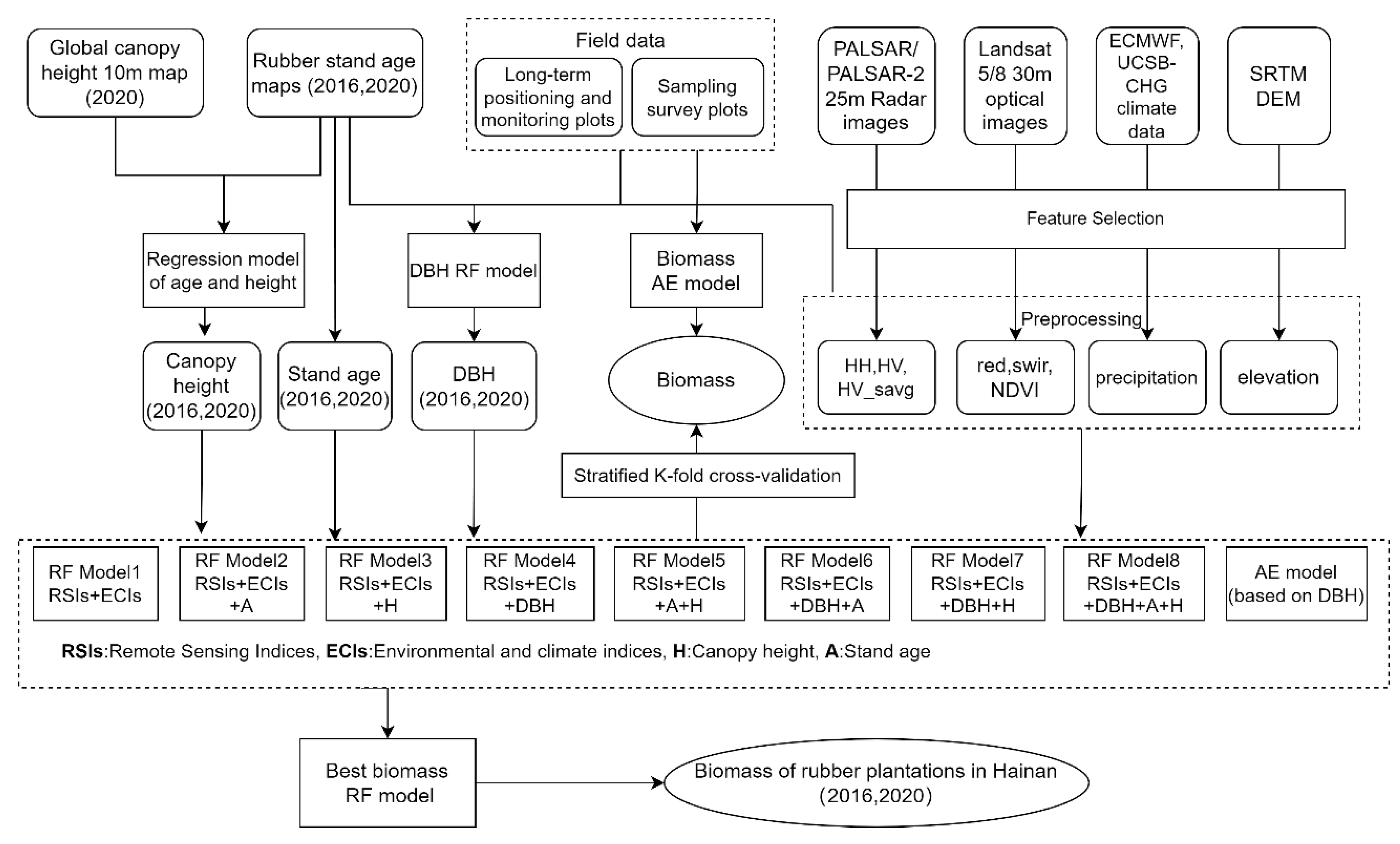
2.3.1. Work Flow

The workflow diagram is depicted in Figure 2, outlining a three-step process: (1) preparation of biomass inversion variables encompassing direct variables, such as RSIs and ECIs, and indirect variables, like canopy height (H) and DBH; (2) evaluation and comparison of various biomass models based on these variables; and (3) identification of the optimal model for estimating rubber plantation biomass in Hainan Island, accompanied by an analysis of its temporal and spatial characteristics. The canopy height for 2016 (the year of the island-wide field investigation) was estimated through the development of a height and stand age model. At present, there is no readily available remote sensing-based model for rubber DBH estimation. We modeled and compared field observations, stand age, RSIs, and ECIs, selecting the optimal model to estimate DBH.

2.3.2. Key Independent Parameter Estimation

Stand Age (A)
The 2020 and 2016 maps of rubber plantations were generated through the utilization of dense optical and radar satellite imagery coupled with a phenology-based decision tree algorithm. The implementation of these techniques yielded an overall classification accuracy of 90%, as reported by [33]. The stand age maps for the years 2016 and 2020 relied on these rubber plantation maps and a comprehensive analysis of long-term time-series images from Landsat and Sentinel-2 satellites beginning in 1987. This analysis followed an algorithm previously outlined [34]. The algorithm’s core principle involves utilizing distinctive features of land-use and land-cover changes during the establishment phase of plantations and the subsequent progression of canopy closure from rubber seedlings to fully mature dense plantations. By employing these parameters, the algorithm can effectively identify the precise year of establishment for rubber plantations. The target year minus the establishment year is the stand age of a rubber plantation in a specific year.
Canopy Height (H)
The canopy height data for the entirety of Hainan Island in 2020 were produced in [30]. This study is considered a milestone in the field as it produced the first global 2020 wall-to-wall canopy height map at 10 m spatial resolution through the integration of GEDI and Sentinel-2 imagery with a probabilistic deep learning model. Given the strong relationship between stand age and canopy height [41], it was judged to be feasible to predict the canopy height of rubber plantations in 2016 based on this relationship and the wall-to-wall canopy height map from 2020. The primary steps included: (1) reclassifying the 2020 stand age map of rubber plantations in 1-year increments, followed by masking of the 2020 canopy height map; (2) performing sampling for each age class map with 50 sample points and extracting the corresponding canopy height for these sample points; (3) computing the percentile mean and standard deviation for the canopy height within a range of 20 to 80 percent (excluding misclassified rubber pixels and canopy height outliers); and (4) constructing a regression model with stand age as the independent variable and average canopy height as the dependent variable.
DBH
The DBH is also closely related to the stand age and the growth environment of rubber trees. By combining the field DBH, stand age (A), canopy height (H), RSIs, and ECIs, we developed and compared three random forest (RF)-based DBH models using Equation (6).
D B H R F = f ( R S I s , E C I s , A | H ) + ε
where D B H R F is the DBH estimated by the random forest algorithm; A | H represents the stand age and canopy height, which were additional independent variables during the test; and ε is the error in the estimated DBH. The Boruta algorithm was used to select optimal independent variables from the RSI and ECI sets for the DBH and subsequent biomass estimation, as the feature selection process is fundamental to any machine learning project [42]. The RF algorithm was selected for DBH estimation due to its general immunity to overfitting and data noise and its widespread use in the remote sensing community [43,44]. Ultimately, the optimal model was chosen to estimate the DBH for rubber plantations for different nominal years.

2.3.3. Biomass Estimation Models

The RF algorithm utilized several independent variables, including RSIs, ECIs, A, H, and DBH. The primary reason for selecting RSIs and ECIs as variable sets was their ease of acquisition and their extensive use in traditional biomass estimation via remote sensing. Moreover, the models were assessed by incorporating A, H, DBH, and their combinations (eight combinations in total; Figure 2) using Equation (7).
B R F = f ( R S I s , E C I s , A & | H & | D B H R F ) + ε
where B R F is the biomass estimated, and A & | H & | D B H R F means adding one or a combination of A , H , and D B H R F to the R S I s and E C I s during model estimation. The RF model’s hyperparameters were set to 100 for the number of trees and 1 for the random state. In addition to the RF models, biomass estimates based on the AE model ( B A E ) using Equations (2) and (8) were compared, utilizing the best D B H R F as an input parameter.
B A E = f ( D B H R F ) + ε

2.4. Accuracy Assessment

Considering the limited availability of field data, this study adopted a k-fold (k = 4 was used herein) cross-validation approach for modeling and evaluation. Plots were stratified into diverse categories based on their biomass (10, 20, 30, 40, 50, 60, 70, 80, 90, 100, 110, and greater than 110 mg/ha), which served as the grouping variable. The sample was subsequently divided into four smaller subsets referred to as folds, utilizing a hierarchical k-fold cross-validation method. This technique refines the conventional k-fold cross-validation method by incorporating a grouping variable, ensuring a roughly even distribution of biomass across folds. During each iteration, k−1 folds were employed for training, while the remaining fold was designated for validation. To evaluate model performance, the R2 and RMSE were implemented as metrics. The performance of various band combinations was compared by calculating their mean values within the k-fold loop.

2.5. Spatial Analysis

The biomass of rubber plantations in different administrative regions (provinces and counties/cities) and topographic environments (with differing elevation and slope) on Hainan Island was examined using the GEE cloud platform. Elevation was segmented into seven groups with bin values of 0, 50, 100, 200, 300, 400, and 600 m. Slope was categorized into seven levels with bin values of 0, 5, 10, 15, 20, and 25°, slightly adjusted based on the technical standard Comprehensive control of soil and water conservation—General rule of planning (GB/T 15772-2008) [45]. Additionally, the spatiotemporal characteristics of biomass changes between 2016 and 2020 were analyzed.

3. Results

3.1. Estimation of Canopy Height and DBH

The canopy height (H)–stand age model is presented in Figure 3a. With increasing stand age over the first 10 years, the height of rubber trees rose dramatically. The growth rate slowed between 10 and 15 years, and after 15 years, the trees’ height increased very slowly. According to logistic curve fitting, the R2 reached 0.95. Figure 3b–d show the DBH models established using three different methods. DBH estimated via RSIs and ECIs displayed a high degree of accuracy for rubber trees around 17 years but had clear tendencies for overestimation for trees younger than 15 years and underestimation for trees older than 20 years. The linear fit demonstrated an R2 of 0.36 and an RMSE of 4.38 cm. When the canopy height or stand age was introduced, the prediction accuracy significantly improved: the scatter points for the observed and predicted DBH were mainly distributed along the 1-to-1 line, while the R2 reached 0.76 and 0.77 and the RMSE decreased to 2.65 cm and 2.60 cm, respectively. Considering that stand age is easier to obtain using remote sensing than canopy height, we finally chose the model with RSIs, ECIs, and stand age as independent variables to estimate DBH.

3.2. Comparison of Different Biomass Estimation Models

The nine biomass models developed with different variables and field data from 2016 are presented in Figure 4. Notably, the model exclusively employing RSIs and ECIs exhibited the lowest accuracy in estimation (R2 = 0.24 and RMSE = 38.36 mg/ha) along with the most substantial estimation bias, particularly for rubber plantations with biomass greater than 100 mg/ha (Figure 4a). However, with the introduction of stand age, a significant improvement in prediction accuracy was observed: R2 increased to 0.77 and RMSE decreased to 21.16 mg/ha. Additionally, scatter points demonstrated a closer alignment along the 1-to-1 line (Figure 4b). Likewise, when solely incorporating canopy height, the model’s prediction accuracy remained comparable to that achieved with stand age (R2 = 0.77 and RMSE = 20.91 mg/ha), while the slope of the linear fit improved from 0.79 to 0.80 (Figure 4c). However, the inclusion of DBH led to a substantial enhancement in model accuracy: R2 increased from 0.77 to 0.97, RMSE decreased to 7.73 mg/ha, and the slope improved from 0.80 to 0.93 (Figure 4d). Furthermore, when simultaneously incorporating two out of three variables (A, DBH, and H), the prediction accuracy of both the models incorporating DBH surpassed that of the model without DBH. The R2 for the former models reached 0.97, while the latter model lagged at a value of 0.77 (Figure 4e–g). Incorporating DBH, A, and H together yielded an identical R2 of 0.97 but with a slightly reduced RMSE of 7.43 mg/ha. However, it is worth noting that the biomass calculated using the AE and DBH (from the best RF model) exhibited lower precision compared to the RF models, with an R2 of 0.67 and an RMSE of 25.43 mg/ha (Figure 4i). Consequently, the RF model utilizing RSIs, ECIs, DBH, A, and H as independent variables was selected as the final biomass model. Utilizing this model, the biomass of rubber plantations in both 2016 and 2020 was determined.

3.3. Spatiotemporal Pattern for Rubber Biomass at City/County Scale in Hainan Island

Figure 5 provides an overview of the spatial distribution of rubber plantation biomass in 2016 and 2020. In 2016, the rubber plantations with a biomass of about 70 mg/ha were mainly located in the northwestern and northern regions of Hainan Island, including Lingao and Changjiang county and northwest of Danzhou city. On the other hand, the central region and southeastern coastal regions had higher biomass for the rubber plantations, typically ranging between 70 mg/ha and 85 mg/ha (Figure 5a). In 2020, there was a significant increase in both the area and biomass of rubber plantations. The rubber acreage increased throughout the island, especially in the northwest and northern regions. Rubber plantations with a biomass of approximately 65 mg/ha or less were found to be more widely distributed in the western region of Danzhou city, the northern region of Changjiang and Ledong county, Haikou city, Ding’an county, and Wenchang city. In most of the remaining areas, the biomass of rubber plantations increased to around 70 mg/ha. The areas with the highest biomass were often distributed in the border areas of different cities and counties, such as the border areas between Chengmai county and Tunchang county, Qiongzhong county, Wuzhishan city, Baisha county, and Wanning city, where the biomass of many of the rubber plantations exceeded 120 mg/ha (Figure 5b).
The average biomass of rubber plantations across different cities and counties changed greatly between 2016 and 2020 (Figure 6a). In 2016, the average biomass was approximately 75 mg/ha. Wuzhishan city, Wanning city, and Sanya city had the highest average biomass of about 84 mg/ha. Conversely, the average biomass in Changjiang county, Dongfang county, Ledong city, and Dingan city was relatively low, approximately 69 mg/ha. With the exception of Baisha, Chengmai city, Danzhou county, and Qiongzhong, the average biomass of rubber plantations in the other 14 cities and counties showed a decreasing trend. Notably, Chengmai city had the highest increase of 5.70 mg/ha, far exceeding the other cities and counties. The cities and counties with remarkable decreases in biomass were Wanning county, Tunchang city, Lingao city, and Dongfang county. In 2020, Qiongzhong county had the highest average biomass of approximately 85 mg/ha, followed by Wuzhishan city and Chengmai county, Baisha city, and Wanning county, which had average biomass exceeding 79 mg/ha. The average biomass in Sanya city, Baoting county, Danzhou city, Lingao county, and Tunchang county was concentrated around 73 mg/ha. Dongfang city and Changjiang county had the lowest average biomass for rubber trees among the 18 cities and counties, with values of 63.81 mg/ha and 63.57 mg/ha, respectively.
Figure 6b demonstrates that the total biomass of the rubber plantations in different cities and counties on Hainan Island varied significantly. Danzhou city had the highest total biomass in both 2016 and 2020, with a value of 1.06 × 10⁷ mg in 2020, which was significantly higher than that of other cities and counties. The growth of rubber plantation biomass in Danzhou city was also very rapid, increasing by about 1.93 × 10⁶ mg. In 2016, the total biomass of rubber plantations in Baisha county, Chengmai county, and Qiongzhong county exceeded 4.00 × 10⁶ mg, with the first two cities and counties also demonstrating significant increases. Additionally, Ledong county, Qionghai city, Tunchang county, and Lingao county had total rubber plantation biomass exceeding 2.00 × 10⁶ mg in 2016. Conversely, Dongfang county and Linshui city had smaller total biomass values of 0.63 × 10⁶ mg and 0.67 × 10⁶ mg, respectively, in 2020. The total biomass of rubber plantations on Hainan Island in 2016 and 2020 was 4.52 × 10⁷ and 5.46 × 10⁷ mg, respectively.

3.4. Topographic Pattern of the Latest Rubber Biomass on Hainan Island

Rubber plantations exhibited notable variability in average biomass across differing elevations and slopes in 2020, as demonstrated in Table 1. The most substantial average biomass was observed in rubber plantations situated at elevations between 400 and 600 m above sea level, which exhibited an average biomass of 86.52 mg/ha. Comparatively, plantations distributed at elevations between 300 and 400 m and 200 and 300 m above sea level displayed average biomasses of 85.74 mg/ha and 84.48 mg/ha, respectively. In contrast, the rubber plantations situated at elevations between 0 and 50 m above sea level displayed the lowest average biomass, with a value of 69.08 mg/ha. The average biomass fluctuated slightly among the various slope regions. Specifically, plantations situated in the flattest areas (<5°) exhibited an average biomass of 74.48 mg/ha, while the highest average biomass, 89.38 mg/ha, was observed in plantations situated in regions with slopes greater than 25°. The average biomass of rubber plantations increased marginally with increases in slope, from 74.48 mg/ha in plantations with slopes less than 5° to 89.38 mg/ha in plantations with slopes above 25°.
This study investigated the total biomass of rubber plantations situated at varying elevations and slopes. The findings reveal that the plantations at elevations of 100–200 m above sea level exhibited the highest total biomass, exceeding 2.3 × 10⁷ mg. Rubber plantations at elevations of 50–100 m and 200–300 m possessed total biomass of 1.41 × 10⁷ mg and 0.97 × 10⁷ mg, respectively. Conversely, plantations at elevations above 600 m had considerably lower total biomass amounting to 0.6 × 10⁵ mg. Furthermore, the total biomass of the rubber plantations progressively diminished with increasing slope. For instance, in the plains with slopes less than 5°, the total biomass approached 2.41 × 10⁷ mg, but it decreased sharply to 1.64 × 10⁷ mg in areas with slopes of 5–10°. Notably, regions with slopes exceeding 25° exhibited significantly lower total biomass for rubber plantations amounting to 1.61 × 10⁶ mg.

4. Discussion

4.1. Biomass Estimation Using Different Variables

Signal saturation is a common problem in estimating forest biomass using optical and SAR remote sensing data [12,46,47]. It has been reported that data saturation may occur when biomass density reaches 100–150 mg/ha in moist tropical forests, depending on the complexity of the forest stand structures caused by biophysical environments [12]. For uniformly planted rubber plantations, many studies have found that the saturation point for the biomass is lower than that in moist tropical forests. For example, saturation occurred at 50 mg/ha with the PALSAR HV band, 40 mg/ha with the WorldView-2 images, and 65 mg/ha with the LS2-based spectral indices [6,48,49]. Therefore, it is difficult to accurately estimate the biomass of rubber plantations solely using traditional predictors, such as spectral bands, vegetation indices, geo-environmental indicators, or their combinations. One of our models demonstrated the a estimation bias using RSIs and ECIs: the biomass of rubber plantations was seriously underestimated when it was greater than about 70 mg/ha, with an R2 of 0.24 and RMSE of 38.36 mg/ha (Figure 4a).
The rate of forest biomass accumulation is closely related to stand age, especially in the transitional stage of forest succession [50,51,52]. For specific species, such as rubber trees, the economic life cycle is about 30 years. During the growth and development stage (<10 years), the biomass increases rapidly with the increase in the stand age and gradually slows down with the increase in latex harvesting time [53]. The stand age of rubber trees in the same plantation is consistent, which brings great convenience to the accurate estimation of biomass and alleviates the problem of signal saturation to a great extent. When the stand age was added to the independent variable sets, the estimation accuracy for biomass was significantly improved (R2 = 0.77, RMSE = 21.16 mg/ha; Figure 4b). However, obtaining a high-precision map of rubber stand age in advance is essential for estimating biomass in large areas. Thanks to the development of remote sensing big data and cloud computing platforms, such as GEE [54], it is now possible to quickly access and analyze decades of remote sensing images and obtain more accurate stand age information for rubber plantations by monitoring changes in land use and rubber tree growth [34,55].
Each rubber plantation also has a similar canopy height, which is another key variable, in addition to DBH, in estimating aboveground biomass on the ground [56,57,58]. Estimating tree canopy heights from traditional optical and radar imagery was also challenging until the GEDI instrument was successfully launched on the International Space Station (ISS) [31]. By producing high-resolution laser-range observations of the Earth’s three-dimensional structure, the GEDI instrument significantly increases the accuracy of the worldwide estimation of tree canopy heights [59]. When canopy height was added in the RF model, the estimation accuracy for rubber plantation biomass also significantly improved (R2 = 0.77 and RMSE = 20.91 mg/ha). Compared to the stand age, the accuracy of biomass estimation was slightly higher after adding the canopy height variable (Figure 4b,c), which could explain the differences in canopy height even though the stand age was the same in the same rubber plantation. The height difference between trees in the same plantation can be obtained through the GEDI, while the stand age monitored through time-series images tends to be the same.
Although canopy height was comparable as a biomass estimator variable to DBH, its contribution was found to be significantly lower than that of DBH when tested in this study. Compared with stand age and canopy height, the RF model with only the DBH variable added had the highest estimation accuracy (Figure 4d; R2 = 0.97 and RMSE = 7.73 mg/ha). In the other four RF models using multivariate combinations of stand age, canopy height, and DBH, the accuracy of the model with the DBH variable was also significantly higher than that of the model without DBH (Figure 4e–g). This could be primarily explained by the fact that DBH is the most important variable in forest biomass estimation [3,60,61]. The biomass used for verification in this study came from Equation (2), a DBH-based AE model. Moreover, there are still many uncertainties regarding the current canopy height products. The GEDI data used for canopy height retrieval were discrete footprint samples with a diameter of about 25 m, and the other areas were obtained from indirect estimation with data from multiple sources, such as Landsat imagery [62]. In addition, high geolocation uncertainty in GEDI data is likely to introduce high uncertainty in canopy height estimation. The horizontal geolocation error for each 25 m footprint center for the first-release GEDI data is within 10 m, but a recent evaluation of GEDI early-mission data for about 8 months showed a horizontal geolocation error of 23.8 m [63,64]. Furthermore, canopy height data are currently only available for the nominal years of 2019 and 2020 [62,65]. To match the 2016 DBH data, the canopy height used to estimate rubber plantation biomass in 2016 was indirectly estimated by the regression model developed with stand age (Figure 3a). Due to this indirect estimation, there were more dependencies among the DBH, stand age, and canopy height, which is also an important reason why the model accuracy could not be significantly improved when multiple variable combinations were added at the same time.

4.2. Spatial Distribution Pattern for Rubber Plantations and Biomass on Hainan Island

Rubber plantations constitute over a quarter of the forested area on Hainan Island, representing the largest forest plantation ecosystem in the region [33]. Therefore, quantifying the biomass of these plantations holds considerable significance for the island. The spatial distribution of rubber biomass on Hainan Island is intricately linked to the timeline of the establishment and the location of rubber plantations (Figure 1). Following a rapid increase in natural rubber prices after 2003, rubber planting areas on the island expanded rapidly, particularly in the western and northern regions [33,66]. Although the southeastern and southern parts of Hainan offer favorable temperature and rainfall conditions for rubber cultivation, the former is prone to frequent severe typhoons, and the latter, as a genuine tropical area, generates more substantial economic returns from the production of tropical fruits rather than rubber trees [67,68,69]. This phenomenon explains the high average biomass in Sanya city in the south during 2016, which subsequently declined significantly in 2020 (Figure 6). There are few new rubber plantations in these areas, resulting in most of the old rubber plantations gradually being felled to plant other tropical fruits. Consequently, the establishment of new rubber plantations along the southeastern coast and in the south is substantially lower in comparison to the western and northern regions.
With regard to alterations in spatial distribution, the extent of rubber plantations in 2020 was markedly greater than in 2016 (Figure 5). This observation may be ascribed to the limitations of existing algorithms, which solely detect rubber plantations exhibiting forest morphological characteristics via remote sensing approximately five years post-establishment [34]. Consequently, the rubber plantations that principally expanded between 2016 and 2020 were established between 2010 and 2015. Despite a precipitous decline in natural rubber prices following their peak in 2011, the enlargement of rubber planting areas persisted due to a temporal disconnect between plantation growth and price oscillations [66,70,71]. For example, statistics indicate that, between 2010 and 2015, newly established rubber plantations on Hainan Island encompassed 128,000 ha (averaging 21,000 ha annually), while this figure diminished to approximately 3200 ha in 2016 [72]. As a result, by the end of 2020, a substantial portion of Hainan Island’s rubber plantations consisted of trees less than 15 years old, displaying relatively low biomass density. The rise in the proportion of young rubber plantations explains the reduced average biomass for rubber plantations in numerous cities and counties in 2020 compared to 2016 (Figure 6). However, the augmented total area of rubber plantations in 2020 contributed to the elevation of total biomass in the majority of cities and counties. The total biomass of rubber plantations island-wide also increased from 4.52 × 10⁷ mg in 2016 to 5.46 × 10⁷ mg in 2020.
Rubber plantations characterized by higher biomass (exceeding 120 mg/ha) are predominantly situated in central mountainous regions and the border areas of different cities and counties (Figure 5). This distribution may be attributed to the elevated expenses associated with short-term, intensive agricultural development in mountainous locales, rendering the cultivation of perennial rubber trees a more favorable option [73]. The considerable costs involved in updating old rubber plantations in these regions facilitate the preservation of older rubber plantations [34]. For example, the top four rubber plantations with the highest average biomass in 2020 were Qiongzhong county, Wuzhishan city, Chenmai county, and Baisha county, three of which have typical mountainous terrain (Figure 6). In addition, border areas often comprise underdeveloped regions with unfavorable geographic conditions, which, in turn, increases the likelihood of maintaining older rubber plantations [74,75].

4.3. Uncertainty Analysis and Potential Application Prospects

The precision of rubber plantation biomass estimation primarily depends on the accurate determination of three variables: DBH, stand age, and canopy height. Remote sensing offers a comparatively more feasible approach for acquiring stand age and canopy height data than obtaining DBH measurements. The estimation of stand age and canopy height involves a relatively comprehensive algorithm that demonstrates notably high accuracy, with an RMSE of approximately 2 years, when sufficient image data are available [34,55]. Nevertheless, the availability of Landsat 5 images prior to 2000 was limited, leading to a scarcity of data sources and consequently affecting the estimation accuracy. With regard to canopy height estimation, significant improvements in accuracy have been achieved through the use of GEDI data [30,62], but it still has high uncertainty due to intrinsic geometric positioning errors associated with the GEDI and the availability of footprint points only. While the indirect estimation of DBH through RSIs, ECIs, stand age, and canopy height displays high accuracy, the employed algorithm lacks clear theoretical significance. Furthermore, tropical regions are characterized by severe landscape fragmentation [25,76], and many rubber plantations are managed by smallholders with limited land area that is not easy to detect, which exacerbates the problems of collecting stand age and canopy height at the spatial resolution level of satellite imagery. Hence, a more advanced nonlinear regression fitting analyzer [77] that can synthetically consider all disturbance factors related to the rubber tree biomass assessment could be developed to raise the accuracy of the final results.
Despite the existence of limitations, the algorithm employed in this study demonstrates promising potential and can be readily applied to other rubber cultivation regions, such as Xishuangbanna in Yunnan province, China, and various Southeast Asian countries. Firstly, the utilization of platforms such as GEE and the availability of extensive time-series big data, such as from Landsat, Sentinel, and SDGSAT-1, enable accurate estimation of rubber stand age [54,78]. Secondly, the canopy height products from 2020 are on a global scale, and canopy height in recent years can be further mapped using the latest LiDAR data acquired from GEDI and GF-7, as well as L-band SAR data, like PALSAR-2 [13]. By incorporating ground survey data to refine the DBH estimation model and biomass allometric equations specific to different regions, it is anticipated that satisfactory accuracy in biomass estimation can be achieved across diverse geographical areas.
Against the backdrop of persistently low natural rubber prices for over a decade and China’s explicit commitment to carbon peaking and carbon neutrality [79,80], the practical significance of large-scale biomass/carbon storage estimation in rubber plantations is becoming increasingly profound. Accurately determining the carbon sink capacity of rubber plantations holds the potential to facilitate carbon trading initiatives and enhance the economic benefits associated with rubber cultivation. For example, implementation of the Verified Carbon Standard (VCS) in forestry carbon sequestration projects within rubber plantations can yield tangible economic advantages for various stakeholders, including rubber farmers, businesses, and government regulators [81]. Hence, with the continuous upgrading of satellite-borne remote sensing techniques and the latest image processing algorithms, the ideological elaboration of carbon stock surveying from the regional scale to the sample-plot scale and then the individual-tree scale could be achieved in the near future [82].

5. Conclusions

Estimating biomass in rubber plantations holds significant scientific and practical implications, but achieving accurate estimations on a large scale remains challenging. This study employed remote sensing images, ground surveys, and key physiological factors, such as stand age and canopy height, to investigate the impact of different predictors and estimation methods on biomass estimation accuracy in rubber plantations. The results demonstrate that incorporating stand age or canopy height factors into the random forest model based on RSIs and ECIs significantly improves biomass prediction accuracy. This approach effectively addresses the signal saturation problem encountered in traditional remote sensing inversion, increasing the R2 value from 0.24 to 0.77. Furthermore, when the DBH—the most widely used variable for biomass estimation using the AE—was added to the model, the prediction accuracy surpassed that obtained when adding stand age or canopy height, resulting in an R2 value of 0.97. However, incorporating two or all of the variables (stand age, canopy height, and DBH) into the model did not yield significant improvements in prediction accuracy as compared to the more straightforward approach using RSIs, ECIs, and DBH.
This study applied the optimal model to estimate biomass in rubber plantations on Hainan Island, China’s second-largest rubber planting region, for the years 2016 and 2020. The results reveal that spatiotemporal biomass distribution patterns closely correlate with rubber plantation distribution and establishment years. Since the onset of the 21st century, the increasing price of natural rubber has prompted the establishment of numerous rubber plantations across the island, particularly in the northwest and northern regions. Consequently, these areas exhibit relatively low biomass densities (e.g., <50 mg/ha). In contrast, older rubber plantations in the central mountainous region and the border areas of different cities and counties feature higher biomass densities (e.g., >120 mg/ha). Although the average biomass in over half of the cities and counties in 2020 was marginally lower than in 2016, the total biomass of rubber plantations in most cities and counties exhibited a clear growth trend due to the expansion of plantation areas. By the end of 2020, the total biomass of rubber plantations on Hainan Island reached 5.46 × 10⁷ mg, emphasizing its substantial value for the carbon cycle on Hainan Island.

Author Contributions

Conceptualization, Z.W. and B.C.; Methodology, X.W., Y.G. and B.C.; Software, X.L., X.W., Y.G. and J.W.; Validation, B.C.; Formal analysis, X.L. and Q.B.; Investigation, R.C. and B.C.; Resources, B.C.; Data curation, X.W. and B.C.; Writing—original draft, X.L.; Writing—review & editing, X.L. and B.C.; Visualization, D.R.; Supervision, T.Y. and G.X.; Project administration, X.L.; Funding acquisition, X.L., Z.W. and B.C. All authors have read and agreed to the published version of the manuscript.

Funding

This research was funded in part by the Hainan Province Science and Technology Special Found (ZDYF2021SHFZ257) and Natural Science Foundation (422CXTD527, 2019RC329), the National Natural Science Foundation of China (42071418), the Earmarked Fund for China Agriculture Research System (CARS-33), and the Innovation and Entrepreneurship Training Project for Undergraduates in Jiangsu Province (202210298044Z).

Acknowledgments

We thank the U.S Geological Survey (USGS) EROS Data Center and JAXA for their data sources and Google for their GEE platform.

Conflicts of Interest

The authors declare no conflict of interest.

References

  1. Yun, T.; Jiang, K.; Li, G.; Eichhorn, M.P.; Fan, J.; Liu, F.; Chen, B.; An, F.; Cao, L. Individual tree crown segmentation from airborne LiDAR data using a novel Gaussian filter and energy function minimization-based approach. Remote Sens. Environ. 2021, 256, 112307. [Google Scholar] [CrossRef]
  2. Yang, Q.; Su, Y.; Hu, T.; Jin, S.; Liu, X.; Niu, C.; Liu, Z.; Kelly, M.; Wei, J.; Guo, Q. Allometry-based estimation of forest aboveground biomass combining LiDAR canopy height attributes and optical spectral indexes. For. Ecosyst. 2022, 9, 100059. [Google Scholar] [CrossRef]
  3. Yang, X.; Blagodatsky, S.; Liu, F.; Beckschäfer, P.; Xu, J.; Cadisch, G. Rubber tree allometry, biomass partitioning and carbon stocks in mountainous landscapes of sub-tropical China. Forest Ecol. Manag. 2017, 404, 84–99. [Google Scholar] [CrossRef]
  4. Koch, B. Status and future of laser scanning, synthetic aperture radar and hyperspectral remote sensing data for forest biomass assessment. ISPRS J. Photogramm. Remote Sens. 2010, 65, 581–590. [Google Scholar] [CrossRef]
  5. Zhang, R.; Zhou, X.; Ouyang, Z.; Avitabile, V.; Qi, J.; Chen, J.; Giannico, V. Estimating aboveground biomass in subtropical forests of China by integrating multisource remote sensing and ground data. Remote Sens. Environ. 2019, 232, 111341. [Google Scholar] [CrossRef]
  6. Chen, B.; Yun, T.; Ma, J.; Kou, W.; Li, H.; Yang, C.; Xiao, X.; Zhang, X.; Sun, R.; Xie, G.; et al. High-Precision Stand Age Data Facilitate the Estimation of Rubber Plantation Biomass: A Case Study of Hainan Island, China. Remote Sens. 2020, 12, 3853. [Google Scholar] [CrossRef]
  7. Tian, X.; Su, Z.; Chen, E.; Li, Z.; van der Tol, C.; Guo, J.; He, Q. Estimation of forest above-ground biomass using multi-parameter remote sensing data over a cold and arid area. Int. J. Appl. Earth Obs. 2012, 14, 160–168. [Google Scholar]
  8. Zolkos, S.G.; Goetz, S.J.; Dubayah, R. A meta-analysis of terrestrial aboveground biomass estimation using lidar remote sensing. Remote Sens. Environ. 2013, 128, 289–298. [Google Scholar] [CrossRef]
  9. Sileshi, G.W. A critical review of forest biomass estimation models, common mistakes and corrective measures. Forest Ecol. Manag. 2014, 329, 237–254. [Google Scholar] [CrossRef]
  10. Chao, Z.; Liu, N.; Zhang, P.; Ying, T.; Song, K. Estimation methods developing with remote sensing information for energy crop biomass: A comparative review. Biomass Bioenergy 2019, 122, 414–425. [Google Scholar] [CrossRef]
  11. Schulze-Brüninghoff, D.; Wachendorf, M.; Astor, T. Remote sensing data fusion as a tool for biomass prediction in extensive grasslands invaded by L. polyphyllus. Remote Sens. Ecol. Conserv. 2021, 7, 198–213. [Google Scholar] [CrossRef]
  12. Lu, D.; Chen, Q.; Wang, G.; Liu, L.; Li, G.; Moran, E. A survey of remote sensing-based aboveground biomass estimation methods in forest ecosystems. Int. J. Digit. Earth. 2014, 9, 63–105. [Google Scholar] [CrossRef]
  13. Thapa, R.B.; Watanabe, M.; Motohka, T.; Shimada, M. Potential of high-resolution ALOS–PALSAR mosaic texture for aboveground forest carbon tracking in tropical region. Remote Sens. Environ. 2015, 160, 122–133. [Google Scholar] [CrossRef]
  14. Zheng, G.; Chen, J.M.; Tian, Q.J.; Ju, W.M.; Xia, X.Q. Combining remote sensing imagery and forest age inventory for biomass mapping. J. Environ. Manag. 2007, 85, 616–623. [Google Scholar] [CrossRef] [PubMed]
  15. Kumar, L.; Sinha, P.; Taylor, S.; Alqurashi, A.F. Review of the use of remote sensing for biomass estimation to support renewable energy generation. J. Appl. Remote Sens. 2015, 9, 97696. [Google Scholar] [CrossRef]
  16. Propastin, P. Modifying geographically weighted regression for estimating aboveground biomass in tropical rainforests by multispectral remote sensing data. Int. J. Appl. Earth Obs. 2012, 18, 82–90. [Google Scholar] [CrossRef]
  17. Lu, D. The potential and challenge of remote sensing-based biomass estimation. Int. J. Remote Sens. 2007, 27, 1297–1328. [Google Scholar] [CrossRef]
  18. Azizan, F.A.; Kiloes, A.M.; Astuti, I.S.; Abdul Aziz, A. Application of Optical Remote Sensing in Rubber Plantations: A Systematic Review. Remote Sens. 2021, 13, 429. [Google Scholar] [CrossRef]
  19. Shidiq, I.P.A.; Ismail, M.H.; Kamarudin, N. Initial results of the spatial distribution of rubber trees in Peninsular Malaysia using remotely sensed data for biomass estimate. IOP Conf. Ser. Earth Environ. Sci. 2014, 18, 12135. [Google Scholar] [CrossRef]
  20. Liu, C.; Pang, J.; Jepsen, M.; Lü, X.; Tang, J. Carbon Stocks across a Fifty Year Chronosequence of Rubber Plantations in Tropical China. Forests 2017, 8, 209. [Google Scholar] [CrossRef] [Green Version]
  21. Liang, Y.; Kou, W.; Lai, H.; Wang, J.; Wang, Q.; Xu, W.; Wang, H.; Lu, N. Improved estimation of aboveground biomass in rubber plantations by fusing spectral and textural information from UAV-based RGB imagery. Ecol. Indic. 2022, 142, 109286. [Google Scholar] [CrossRef]
  22. Suratman, M.N.; Bull, G.Q.; Leckie, D.G.; LeMay, V.; Marshall, P.L. Modelling attributes of rubberwood (Hevea brasiliensis) stands using spectral radiance recorded by Landsat Thematic Mapper in Malaysia. IEEE Int. Geosci. Remote Sens. Symp. 2002, 4, 2087–2090. [Google Scholar]
  23. Simon, J.N.; Nuthammachot, N.; Titseesang, T.; Okpara, K.E.; Techato, K. Spatial Assessment of Para Rubber (Hevea brasiliensis) above Ground Biomass Potentials in Songkhla Province, Southern Thailand. Sustainability 2021, 13, 9344. [Google Scholar] [CrossRef]
  24. Kou, W.; Xiao, X.; Dong, J.; Gan, S.; Zhai, D.; Zhang, G.; Qin, Y.; Li, L. Mapping Deciduous Rubber Plantation Areas and Stand Ages with PALSAR and Landsat Images. Remote Sens. 2015, 7, 1048–1073. [Google Scholar] [CrossRef] [Green Version]
  25. Zhai, D.; Dong, J.; Cadisch, G.; Wang, M.; Kou, W.; Xu, J.; Xiao, X.; Abbas, S. Comparison of Pixel- and Object-Based Approaches in Phenology-Based Rubber Plantation Mapping in Fragmented Landscapes. Remote Sens. 2018, 10, 44. [Google Scholar] [CrossRef] [Green Version]
  26. Wu, J.; Zeng, H.; Zhao, F.; Chen, C.; Liu, W.; Yang, B.; Zhang, W. Recognizing the role of plant species composition in the modification of soil nutrients and water in rubber agroforestry systems. Sci. Total Environ. 2020, 723, 138042. [Google Scholar] [CrossRef]
  27. Yang, J.; Xu, J.; Zhai, D. Integrating Phenological and Geographical Information with Artificial Intelligence Algorithm to Map Rubber Plantations in Xishuangbanna. Remote Sens. 2021, 13, 2793. [Google Scholar] [CrossRef]
  28. Chen, B.; Wu, Z.; Wang, J.; Dong, J.; Guan, L.; Chen, J.; Yang, K.; Xie, G. Spatio-temporal prediction of leaf area index of rubber plantation using HJ-1A/1B CCD images and recurrent neural network. ISPRS J. Photogramm. Remote Sens. 2015, 102, 148–160. [Google Scholar] [CrossRef]
  29. Adam, M.; Urbazaev, M.; Dubois, C.; Schmullius, C. Accuracy Assessment of GEDI Terrain Elevation and Canopy Height Estimates in European Temperate Forests: Influence of Environmental and Acquisition Parameters. Remote Sens. 2020, 12, 3948. [Google Scholar] [CrossRef]
  30. Nico, L.; Walter, J.; Konrad, S.; Jan Dirk, W. A high-resolution canopy height model of the Earth. arXiv 2022, arXiv:2204.08322. [Google Scholar]
  31. Sun, M.; Cui, L.; Park, J.; García, M.; Zhou, Y.; Silva, C.A.; He, L.; Zhang, H.; Zhao, K. Evaluation of NASA’s GEDI Lidar Observations for Estimating Biomass in Temperate and Tropical Forests. Forests 2022, 13, 1686. [Google Scholar] [CrossRef]
  32. Hainan Provincial Bureau of Statistics; Survey Office of National Bureau of Statistics in Hainan. Hainan Statistical Yearbook 2020; China Statistics Press: Beijing, China, 2020. [Google Scholar]
  33. Li, G.; Kou, W.; Chen, B.; Wu, Z.; Zhang, X.; Yun, T.; Ma, J.; Sun, R.; Li, Y. Spatio-temporal changes of rubber plantations in Hainan Island over the past 30 years. J. Nanjing For. Univ. (Nat. Sci. Ed.) 2023, 47, 189–198. [Google Scholar]
  34. Chen, B.; Xiao, X.; Wu, Z.; Yun, T.; Kou, W.; Ye, H.; Lin, Q.; Doughty, R.; Dong, J.; Ma, J.; et al. Identifying Establishment Year and Pre-Conversion Land Cover of Rubber Plantations on Hainan Island, China Using Landsat Data during 1987–2015. Remote Sens. 2018, 10, 1240. [Google Scholar] [CrossRef] [Green Version]
  35. Tucker, C.J. Red and photographic infrared linear combinations for monitoring vegetation. Remote Sens. Environ. 1979, 8, 127–150. [Google Scholar] [CrossRef] [Green Version]
  36. Huete, A.; Didan, K.; Miura, T.; Rodriguez, E.P.; Gao, X.; Ferreira, L.G. Overview of the radiometric and biophysical performance of the MODIS vegetation indices. Remote Sens. Environ. 2002, 83, 195–213. [Google Scholar] [CrossRef]
  37. Xiao, X.; Boles, S.; Liu, J.; Zhuang, D.; Liu, M. Characterization of forest types in Northeastern China, using multi-temporal SPOT-4 VEGETATION sensor data. Remote Sens. Environ. 2002, 82, 335–348. [Google Scholar] [CrossRef]
  38. Hashim, I.C.; Shariff, A.R.M.; Bejo, S.K.; Muharam, F.M.; Ahmad, K. Machine-Learning Approach Using SAR Data for the Classification of Oil Palm Trees That Are Non-Infected and Infected with the Basal Stem Rot Disease. Agronomy 2021, 11, 532. [Google Scholar] [CrossRef]
  39. Tan, K.P.; Kanniah, K.D.; Cracknell, A.P. Use of UK-DMC 2 and ALOS PALSAR for studying the age of oil palm trees in southern peninsular Malaysia. Int. J. Remote Sens. 2013, 34, 7424–7446. [Google Scholar] [CrossRef]
  40. Muñoz-Sabater, J.; Dutra, E.; Agustí-Panareda, A.; Albergel, C.; Arduini, G.; Balsamo, G.; Boussetta, S.; Choulga, M.; Harrigan, S.; Hersbach, H.; et al. ERA5-Land: A state-of-the-art global reanalysis dataset for land applications. Earth Syst. Sci. Data 2021, 13, 4349–4383. [Google Scholar] [CrossRef]
  41. Vastaranta, M.; Niemi, M.; Wulder, M.A.; White, J.C.; Nurminen, K.; Litkey, P.; Honkavaara, E.; Holopainen, M.; Hyyppä, J. Forest stand age classification using time series of photogrammetrically derived digital surface models. Scand. J. Forest Res. 2016, 31, 194–205. [Google Scholar] [CrossRef]
  42. Kursa, M.B.; Rudnicki, W.R. Feature selection with the Boruta package. J. Stat. Softw. 2010, 36, 1–13. [Google Scholar] [CrossRef] [Green Version]
  43. Guo, Y.; Li, Z.; Zhang, X.; Chen, E.; Bai, L.; Tian, X.; He, Q.; Feng, Q.; Li, W. Optimal Support Vector Machines for Forest Above-ground Biomass Estimation from Multisource Remote Sensing Data. In Proceedings of the 2012 IEEE International Geoscience and Remote Sensing Symposium, Munich, Germany, 22–27 July 2012. [Google Scholar]
  44. Pierrat, Z.A.; Bortnik, J.; Johnson, B.; Barr, A.; Magney, T.; Bowling, D.R.; Parazoo, N.; Frankenberg, C.; Seibt, U.; Stutz, J. Forests for forests: Combining vegetation indices with solar-induced chlorophyll fluorescence in random forest models improves gross primary productivity prediction in the boreal forest. Environ. Res. Lett. 2023, 17, 175006. [Google Scholar] [CrossRef]
  45. GB/T 15772-2008; General Rule of Planning for Comprehensive Control of Soil and Water Conservation. Standardization Administration of the People’s Republic of China: Beijing, China, 2009.
  46. Meng, S.; Pang, Y.; Zhang, Z.; Jia, W.; Li, Z. Mapping Aboveground Biomass using Texture Indices from Aerial Photos in a Temperate Forest of Northeastern China. Remote Sens. 2016, 8, 230. [Google Scholar] [CrossRef] [Green Version]
  47. Wulder, M.A.; White, J.C.; Nelson, R.F.; Næsset, E.; Ørka, H.O.; Coops, N.C.; Hilker, T.; Bater, C.W.; Gobakken, T. Lidar sampling for large-area forest characterization: A review. Remote Sens. Environ. 2012, 121, 196–209. [Google Scholar] [CrossRef] [Green Version]
  48. Avtar, R.; Suzuki, R.; Sawada, H. Natural forest biomass estimation based on plantation information using PALSAR data. PLoS ONE 2014, 9, e86121. [Google Scholar] [CrossRef] [PubMed]
  49. Yasen, K.; Koedsin, W. Estimating Aboveground Biomass of Rubber Tree Using Remote Sensing in Phuket Province, Thailand. J. Med. Bioeng. 2015, 4, 451–456. [Google Scholar] [CrossRef]
  50. Li, H.; Li, C.; Zha, T.; Liu, J.; Jia, X.; Wang, X.; Chen, W.; He, G. Patterns of biomass allocation in an age-sequence of secondary Pinus bungeana forests in China. Forest. Chron. 2014, 90, 169–176. [Google Scholar] [CrossRef]
  51. Yang, B.; Xue, W.; Yu, S.; Zhou, J.; Zhang, W. Effects of Stand Age on Biomass Allocation and Allometry of Quercus Acutissima in the Central Loess Plateau of China. Forests 2019, 10, 41. [Google Scholar] [CrossRef] [Green Version]
  52. Xiang, W.; Li, L.; Ouyang, S.; Xiao, W.; Zeng, L.; Chen, L.; Lei, P.; Deng, X.; Zeng, Y.; Fang, J.; et al. Effects of stand age on tree biomass partitioning and allometric equations in Chinese fir (Cunninghamia lanceolata) plantations. Eur. J. Forest Res. 2021, 140, 317–332. [Google Scholar] [CrossRef]
  53. Cao, J.; Jiang, J.; Lin, W.; Xie, G.; Tao, Z. Biomass of Hevea Clone PR107. Chin. J. Trop. Agric. 2009, 29, 1–8. [Google Scholar]
  54. Gorelick, N.; Hancher, M.; Dixon, M.; Ilyushchenko, S.; Thau, D.; Moore, R. Google Earth Engine: Planetary-scale geospatial analysis for everyone. Remote Sens. Environ. 2017, 202, 18–27. [Google Scholar] [CrossRef]
  55. Beckschäfer, P. Obtaining rubber plantation age information from very dense Landsat TM & ETM + time series data and pixel-based image compositing. Remote Sens. Environ. 2017, 196, 89–100. [Google Scholar]
  56. Wang, M.; Sun, R.; Xiao, Z. Estimation of Forest Canopy Height and Aboveground Biomass from Spaceborne LiDAR and Landsat Imageries in Maryland. Remote Sens. 2018, 10, 344. [Google Scholar] [CrossRef] [Green Version]
  57. Wang, D.; Xin, X.; Shao, Q.; Brolly, M.; Zhu, Z.; Chen, J. Modeling Aboveground Biomass in Hulunber Grassland Ecosystem by Using Unmanned Aerial Vehicle Discrete Lidar. Sensors 2017, 17, 180. [Google Scholar] [CrossRef] [Green Version]
  58. Popescu, S.C.; Zhao, K.; Neuenschwander, A.; Lin, C. Satellite lidar vs. small footprint airborne lidar: Comparing the accuracy of aboveground biomass estimates and forest structure metrics at footprint level. Remote Sens. Environ. 2011, 115, 2786–2797. [Google Scholar] [CrossRef]
  59. Dorado-Roda, I.; Pascual, A.; Godinho, S.; Silva, C.; Botequim, B.; Rodríguez-Gonzálvez, P.; González-Ferreiro, E.; Guerra-Hernández, J. Assessing the Accuracy of GEDI Data for Canopy Height and Aboveground Biomass Estimates in Mediterranean Forests. Remote Sens. 2021, 13, 2279. [Google Scholar] [CrossRef]
  60. Keller, M.; Palace, M.; Hurtt, G. Biomass estimation in the Tapajos National Forest, Brazil: Examination of sampling and allometric uncertainties. Forest Ecol. Manag. 2001, 154, 371–382. [Google Scholar] [CrossRef]
  61. Yen, T. Culm height development, biomass accumulation and carbon storage in an initial growth stage for a fast-growing moso bamboo (Phyllostachy pubescens). Bot. Stud. 2016, 57, 10. [Google Scholar] [CrossRef] [PubMed] [Green Version]
  62. Potapov, P.; Li, X.; Hernandez-Serna, A.; Tyukavina, A.; Hansen, M.C.; Kommareddy, A.; Pickens, A.; Turubanova, S.; Tang, H.; Silva, C.E.; et al. Mapping global forest canopy height through integration of GEDI and Landsat data. Remote Sens. Environ. 2021, 253, 112165. [Google Scholar] [CrossRef]
  63. Beck, J.; Wirt, B.; Luthcke, S.; Hofton, M.; Armston, J. Global Ecosystem Dynamics Investigation (GEDI) Level 02 User Guide Version 2.0; US Geological Survey, Earth Resources Observation and Science Center: Sioux Falls, SD, USA, 2021. [Google Scholar]
  64. Dubayah, R.; Blair, J.B.; Goetz, S.; Fatoyinbo, L.; Hansen, M.; Healey, S.; Hofton, M.; Hurtt, G.; Kellner, J.; Luthcke, S.; et al. The Global Ecosystem Dynamics Investigation: High-resolution laser ranging of the Earth’s forests and topography. Sci. Remote Sens. 2020, 1, 100002. [Google Scholar] [CrossRef]
  65. Lang, N.; Kalischek, N.; Armston, J.; Schindler, K.; Dubayah, R.; Wegner, J.D. Global canopy height regression and uncertainty estimation from GEDI LIDAR waveforms with deep ensembles. Remote Sens. Environ. 2022, 268, 112760. [Google Scholar] [CrossRef]
  66. Mo, Y. Supply and Demand Situation and Risk Analysis of Natural Rubber. China Trop. Agric. 2019, 2, 4–6. [Google Scholar]
  67. Huang, H.; Yang, Z.; Wang, C.; Zhang, J.; Zhang, Y.; Zhang, M. Evaluation of typhoon disaster risk for Hevea brasiliensis in Hainan island. J. Meteorol. Environ. 2019, 35, 130–136. [Google Scholar]
  68. Chen, B.; Cao, J.; Wang, J.; Wu, Z.; Tao, Z.; Chen, J.; Yang, C.; Xie, G. Estimation of rubber stand age in typhoon and chilling injury afflicted area with Landsat TM data: A case study in Hainan Island, China. Forest Ecol. Manag. 2012, 274, 222–230. [Google Scholar] [CrossRef]
  69. Gu, X.; Chen, B.; Yun, T.; Li, G.; Wu, Z.; Kou, W. Spatio-temporal Changes of Forest in Hainan Island from 2007 to 2018 Based on Multi-source Remote Sensing Data. Chin. J. Trop. Crops 2022, 43, 418–429. [Google Scholar]
  70. Grogan, K.; Pflugmacher, D.; Hostert, P.; Mertz, O.; Fensholt, R. Unravelling the link between global rubber price and tropical deforestation in Cambodia. Nature Plants. 2019, 5, 47–53. [Google Scholar] [CrossRef]
  71. Zhai, D.; Xu, J.; Dai, Z.; Cannon, C.H.; Grumbine, R.E. Increasing tree cover while losing diverse natural forests in tropical Hainan, China. Reg. Environ. Chang. 2014, 14, 611–621. [Google Scholar] [CrossRef]
  72. Hainan Provincial Bureau of Statistics; Survey Office of National Bureau of Statistics in Hainan. Hainan Statistical Yearbook 2017; China Statistics Press: Beijing, China, 2017. [Google Scholar]
  73. Foley, J.A.; Ramankutty, N.; Brauman, K.A.; Cassidy, E.S.; Gerber, J.S.; Johnston, M.; Mueller, N.D.; O’Connell, C.; Ray, D.K.; West, P.C.; et al. Solutions for a cultivated planet. Nature 2011, 478, 337–342. [Google Scholar] [CrossRef] [Green Version]
  74. Ahrends, A.; Hollingsworth, P.M.; Ziegler, A.D.; Fox, J.M.; Chen, H.; Su, Y.; Xu, J. Current trends of rubber plantation expansion may threaten biodiversity and livelihoods. Glob. Environ. Chang. 2015, 34, 48–58. [Google Scholar] [CrossRef]
  75. Anderson, J.; O’Dowd, L. Borders, Border Regions and Territoriality: Contradictory Meanings, Changing Significance. Reg. Stud. 1999, 33, 593–604. [Google Scholar] [CrossRef]
  76. Taubert, F.; Fischer, R.; Groeneveld, J.; Lehmann, S.; Müller, M.S.; Rödig, E.; Wiegand, T.; Huth, A. Global patterns of tropical forest fragmentation. Nature 2018, 554, 519–522. [Google Scholar] [CrossRef] [PubMed]
  77. Zhu, F.; Chen, X.; Chen, S.; Zheng, W.; Ye, W. Relative margin induced support vector ordinal regression. Expert Syst. Appl. 2023, 231, 120766. [Google Scholar] [CrossRef]
  78. Tamiminia, H.; Salehi, B.; Mahdianpari, M.; Quackenbush, L.; Adeli, S.; Brisco, B. Google Earth Engine for geo-big data applications: A meta-analysis and systematic review. ISPRS J. Photogramm. Remote Sens. 2020, 164, 152–170. [Google Scholar] [CrossRef]
  79. Wei, Y.; Chen, K.; Kang, J.; Chen, W.; Wang, X.; Zhang, X. Policy and Management of Carbon Peaking and Carbon Neutrality: A Literature Review. Engineering 2022, 14, 52–63. [Google Scholar] [CrossRef]
  80. Zeng, X.; Huang, H. Development and Prospects of Natural Rubber Technology in China. China Tropical Agriculture. China Trop. Agric. 2021, 1, 25–30. [Google Scholar]
  81. von Avenarius, A.; Devaraja, T.; Kiesel, R. An Empirical Comparison of Carbon Credit Projects under the Clean Development Mechanism and Verified Carbon Standard. Climate 2018, 6, 49. [Google Scholar] [CrossRef] [Green Version]
  82. Wang, Y.; Yang, X.; Zhang, L.; Fan, X.; Ye, Q.; Fu, L. Individual tree segmentation and tree-counting using supervised clustering. Comput. Electron. Agric. 2023, 205, 107629. [Google Scholar] [CrossRef]
Figure 1. Spatial distribution map for rubber plantations and sample plots in Hainan Island: (a) map showing the year of establishment of rubber plantations overlayed with sampling plots, (b) plots for long-term monitoring, and (c) typical photo of rubber plantation.
Remotesensing 15 03447 g001
Figure 2. Workflow of the study.
Remotesensing 15 03447 g002
Figure 3. Models for estimating canopy height and DBH: (a) model relating canopy height to stand age and (bd) models for predicting DBH using different independent variables (RSIs, ECIs, stand age (A), and canopy height (H)).
Remotesensing 15 03447 g003
Figure 4. Comparison of various biomass models: (ah) models developed with different combinations variables (RSIs, ECIs, A, H, and DBH); (i) model based on the AE model with DBH.
Remotesensing 15 03447 g004
Figure 5. The spatial distribution of rubber plantation biomass on Hainan Island: (a) 2016 and (b) 2020.
Remotesensing 15 03447 g005
Figure 6. City/county-level rubber plantation biomass on Hainan Island: (a) average and (b) total biomass.
Remotesensing 15 03447 g006
Table 1. The average and total biomass of rubber plantations at different elevations and slopes on Hainan Island in 2020.
Elevation (m)0–5050–100100–200200–300300–400400–600>600
Biomass (mg/ha)69.0875.1779.0284.4885.7486.5282.34
Biomass (×106 mg)4.8314.0523.39.73.951.850.06
Slope (°)0–55–1010–1515–2020–25>25
Biomass (mg/ha)74.4878.4183.3386.0987.5489.38
Biomass (×106 mg)24.0916.358.134.842.721.61
Disclaimer/Publisher’s Note: The statements, opinions and data contained in all publications are solely those of the individual author(s) and contributor(s) and not of MDPI and/or the editor(s). MDPI and/or the editor(s) disclaim responsibility for any injury to people or property resulting from any ideas, methods, instructions or products referred to in the content.

