Discarding–Recovering and Co-Evolution Mechanisms Based Evolutionary Algorithm for Hyperspectral Feature Selection

Abstract

With the improvement of spectral resolution, the redundant information in the hyperspectral imaging (HSI) datasets brings computational, analytical, and storage complexities. Feature selection is a combinatorial optimization problem, which selects a subset of feasible features to reduce the dimensionality of data and decrease the noise information. In recent years, the evolutionary algorithm (EA) has been widely used in feature selection, but the diversity of agents is lacking in the population, which leads to premature convergence. In this paper, a feature selection method based on discarding–recovering and co-evolution mechanisms is proposed with the aim of obtaining an effective feature combination in HSI datasets. The feature discarding mechanism is introduced to remove redundant information by roughly filtering the feature space. To further enhance the agents’ diversity, the reliable information interaction is also designed into the co-evolution mechanism, and if detects the event of stagnation, a subset of discarded features will be recovered using adaptive weights. Experimental results demonstrate that the proposed method performs well on three public datasets, achieving an overall accuracy of 92.07%, 92.36%, and 98.01%, respectively, and obtaining the number of selected features between 15% and 25% of the total.

1. Introduction

The advancement of hyperspectral remote sensing leads to its widespread use in scanning continuous, narrow spectral bands, as it enables the acquisition of information on the reflection or radiation spectrum of objects at various wavelengths [1,2,3]. Digital number (DN) or reflectance value is considered as the feature value for each band and represented as a feature vector. However, there is a large amount of redundant information collected through hyperspectral imaging (HSI) with the electromagnetic spectrum and visible light infrared technology, resulting in high dimensionality [4]. In essence, data dimensionality reduction helps to trim the redundancy and noise [5] and improves classification accuracy, which has become an important topic in the processing of HSI datasets.

Generally, there are two methods for removing the redundancy of the dataset: feature extraction and feature selection. Feature extraction involves the linear or nonlinear transformation of the original high-dimensional features, such as combining different features into a new feature set [6], where the features lose their original physical meaning. Feature selection involves selecting the most representative feature combination from the dataset; it detects representative features and decreases redundant information or noise from data, which improves classification accuracy and enhances comprehensibility [7]. Due to the difficulty in interpreting selected features from feature extraction, feature selection is widely used in the processing of HSI datasets.

There are three feature selection strategies based on the search rule, namely, filter, wrapper, and embedded [8]. The filtering strategy analyzes each feature using a proxy measure [9] and selects a combination with a specified number of features based on the score ranking. However, the score only reflects the correlation with labels, ignoring the feature interactivity that some feature with a low correlation to labels provides greater performance improvement than those with a high correlation to labels. The wrapper strategy combines the process of feature selection with the agent to identify an appropriate combination of features. However, this strategy requires a continuous measure of the feature combination, resulting in high computational complexity and inadequate generalization ability [10]. The embedded strategy selects features in the learning process [11,12], and incorporates the feature selection in training, avoiding the overfitting that may occur in other strategies by adjusting the weights of features. The embedded strategy is usually combined with some iterative searching; the weight is used to guide the next iteration.

Evolutionary algorithm (EA), which mimics the adaptation and survival of the fittest observed in living organisms in nature, uses the searched heuristic information as the guidance; the genetic material of these combinations is then assembled to create new offspring, and the process is repeated over many generations to allow the population evolves towards better solutions [13]. Traditional EAs update the genetic material through mutation and crossover operations, which are then passed to the next generation. However, those algorithms only consider the stochasticity between agents, but not the similarity between them, which will lead to the occurrence of premature convergence and overfitting phenomena [14,15]. To address these limitations, distance-based EAs have been proposed; these algorithms are designed to calculate the distance between agents to determine their similarity and select some of them for crossover and mutation based on the similarity [16,17,18,19,20], thereby helping to maintain diversity in the population and prevent premature convergence. Nonetheless, due to the absence of competition or collaboration, the information interaction between agents is insufficient, making it difficult for the EA to overcome local optima and leading to stagnation in the iterative process.

The co-evolution mechanism is a means of enhancing information interaction ability. Due to its robustness, this mechanism has received extensive attention and has been widely used in various fields, including natural language processing and image retrieval [21,22]. By combining EA, the co-evolution mechanism improves the search efficiency of the EA in feature selection to some extent [23,24,25]. It divides the original feature set into many subsets; subpopulations are formed based on the agents generated by these subsets, then this mechanism enhances the diversity by information interacting between the agents in different subpopulations. However, the current information interaction only takes into account exchanging the solution encoding with weak representation, leading to the low diversity of agents and the subpopulation imbalance where some agents obtain better combinations after searching than others most of the time. Therefore, a co-evolution mechanism with prominent reliability is necessary to be further searched to fully realize its potential.

In this paper, a feature selection method based on discarding–recovering and co-evolution mechanisms is proposed to obtain a reduced feature combination of the HSI datasets with adequate accuracy. The feature discarding mechanism is introduced to filter out redundant features from the original dataset. Moreover, the co-evolution mechanism is combined with EA to enhance the diversity of agents, and a reliable information interaction is used to enable collaborative search between agents and help EA to jump out of the local optima. To avoid the erroneous discarding of the interactive features that have a low correlation with labels and improve the generalization ability, feature recovery is introduced to raise the probability of discarded features. The purpose of this work is that propose a feature selection method to select an effective feature combination and decrease the redundant information in HSI datasets. The co-evolution mechanism is utilized to promote the subpopulations of EA consistently. Moreover, the feature discarding and recovering mechanisms are used to avoid meaningless searching and enhance the generalization ability. The main contributions of this work are listed as follows:

(1)

The discarding–recovering mechanism is designed to enhance the generalization ability and decrease the computational load, which filters the original feature space and recovers some features into the population.

(2)

The co-evolution mechanism is combined with EA, which divides two subpopulations to co-evolve and utilizes reliable information interaction to enhance the diversity of agents in subpopulations.

(3)

A feature selection method based on discarding–recovering and co-evolution mechanisms is proposed to obtain an effective feature combination, which has a prominent performance in HSI datasets.

The rest of this paper is structured as follows: Section 2 provides the background information; Section 3 details the proposed feature selection method; Section 4 presents the experimental results from different perspectives; Section 5 exhibits the discussion of the proposed method and Section 6 outlines the conclusions.

2. Related Work

2.1. The Feature Selection Method Based on Distance-Based EA

The feature selection method based on distance-based EA has received much attention for its effectiveness in data dimensionality reduction, as it iteratively uses heuristic information to guide the next iteration. Wu et al. [26] developed the particle swarm optimizer (PSO) to reduce the dimensionality of the HSI dataset, where the chaotic sequence was used to initialize the feature space, helping PSO jump out of local optima. Su et al. [27] proposed a novel feature selection method based on the improved firefly algorithm (FA), which largely outperformed the conventional covariance method. Xie et al. [28] proposed a comprehensive feature selection method based on the artificial bee colony algorithm (ABC) and subspace division, achieving prominent overall classification accuracy (OA) while reducing a small amount of redundant information. Wang et al. [29] presented an optimized feature selection method based on the grey wolf optimizer (GWO) in the HSI dataset, which uses the adaptive weight to regulate the balance between optimal individuals and chaos operation to set correlative parameters. Tschannerl et al. [30] proposed an unsupervised feature selection method based on information theory and a modified discrete gravitational search algorithm (GSA), obtaining a more informative subset of features. However, with the increase of the data dimensionality, the ability of EA for further dimensionality reduction gradually decreases since the monotonous agents, leading to the selected feature combination, are redundant to some extent, and distinguishing between the approximate labels is difficult.

2.2. The Co-Evolution Mechanism of Feature Selection

The co-evolution mechanism uses the “divide and conquer” approach to divide the population, identify the current optimal subsets in the feature space, and eventually join them together into a global subset. Song et al. [31] proposed an adaptive subpopulation size adjustment mechanism based on co-evolution and a feature importance-oriented spatial partition strategy, decreasing the calculating time of particle evaluation and providing a competitive solution for the feature selection of high-dimensional data. Zhao et al. [32] proposed a multiple populations co-evolution mechanism and multi-stage interaction learning (OL) mechanism to fully search the prospective features in the stagnant state and increase the possibility of jumping out of local optima. Zhou et al. [33] proposed a feature selection method based on a cooperative co-evolution mechanism (CC-DFS). This method used a heterogeneous model to search for feature combinations with cut-off points and feature combinations without cut-off points, resulting in improved performance and generalization ability. Rashid et al. [34] proposed a feature selection method based on a cooperative co-evolution mechanism and random feature grouping (CC-RFG). Three ways were introduced to decompose the feature set dynamically to ensure the interactive features were divided into the same subpopulation. However, the above co-evolution mechanisms for feature selection only exchange the feature combination with weak representation, leading to the difficulty of regulating those features.

2.3. Motivation

To tackle the problem of the EA in data dimensionality reduction caused by the large feature space and redundant information, the preliminary filtering of the original feature set is required, which helps to decrease the redundancy information of the dataset. To further enhance the performance and effectiveness of EA, it is important to speed up the search process, increase the diversity of agents, and facilitate effective information interaction to improve the quality of the selected features.

Regarding the co-evolution mechanism, when agents from different subpopulations interact, they exchange information that is likely to improve the OA or decrease the number of selected features searched by agents. However, if weak features are not considered, it will lead to an imbalance problem. To overcome these limitations, increasing the probability of selecting the weak features and promoting diverse information interaction between agents is necessary. By this, the co-evolution mechanism achieves a balanced and effective optimization process, leading to a prominent result in HSI datasets.

In all, to improve search efficiency, it is necessary to remove the redundant features in the original feature set while recovering some of these features when detecting update stagnation. Additionally, the co-evolution mechanism is introduced to enhance the diversity of agents in corresponding subpopulations, given that interaction with diverse information is required to maintain the balance between subpopulations. All these measures help improve the performance and stability of agents in feature selection, making them more effective for real-world applications.

3. The Proposed Method

There is a certain of redundant information in the HSI dataset, and the performance in the reduction of data dimensionality has room to improve for EA. As a result, the feature discarding mechanism is implemented that uses some measure criteria to roughly filter the feature space, and the co-evolution mechanism is utilized to divide the population and take the reliable information interaction between agents to enhance the generalization ability. During the iteration process, if a stagnation phenomenon is detected, it is likely caused by the previous erroneous discarding of the interactive features, so the feature recovering mechanism is detonated to increase the selected probability of weak features by adaptive weights, and some of them will be recovered into the subpopulations.

3.1. The Feature Discarding Mechanism

Given the high degree of redundant features in the original dataset, removing it on a large scale is necessary. This eliminates the need for a thorough analysis of each feature and allows for a fast return of selected features. The evaluation measure for each feature is defined as follows:

$$S^n=\sum _{K=1}^n{X}_n^K,n=\mathrm{1,2},3\dots \dots m$$

(1)

$$X_n^K=\frac{2}{\left|{\left({\theta }^k\right)}^{T}H{\theta }^k-{\left({\theta }^k\right)}^T{H}^{(-t)}{\theta }^k\right|}$$

(2)

where $H\in {\mathbb{R}}^{n\times n}$, $H_{i,j}=kernel\left(x_i,x_j\right)$, and $H^{\left(-t\right)}=kernel\left(x_i^{-t},x_j^{-t}\right)$ the $\left(-t\right)$ indicates that $t^{th}$ feature is discarded. Note that $kernel\left(x_i,x_j\right)$ is the kernel function mapped to a high-dimensional space, and $\theta$ represents the optimized parameters obtained from the SVM-based classifier [35].

The feature discarding mechanism, which is based on forward filtering and reverse learning, is implemented to obtain the ranking of feature scores using Equations (1) and (2), drops the specified number of features, and recovers groups of features with low score ranking through reverse learning [36]. In addition, to improve the generalization ability, the feature discarding mechanism calculates the compromise value of recovery groups [37]. The mathematical model is defined as follows:

$$U_i=\underset{1<k<m}{\mathrm{m}\mathrm{a}\mathrm{x}}\left[w_k\frac{o_k^{\mathrm{*}}-x_{ik}}{o_k^{\mathrm{*}}-o_k^{-}}\right],R_i=\sum _{k=1}^m{w}_k\frac{o_k^{\mathrm{*}}-x_{ik}}{o_k^{\mathrm{*}}-o_k^{-}}$$

(3)

$$Q_i=\frac{v\left(R_i-R^{\mathrm{*}}\right)}{R^{-}-R^{\mathrm{*}}}+\frac{(1-v)\left(U_i-U^{\mathrm{*}}\right)}{U^{-}-U^{\mathrm{*}}}$$

(4)

where $R_i$ and $U_i$ denote the utility measure and the regret measure between $m$ features, respectively, $W$ is the weight vector, ${ O}_k^{*}$ is the maximum value of $k^{th}$ feature of the decision matrix, $O_k^{-}$ is the minimum value of $k^{th}$ feature of the decision matrix. $R^{*}$ and $U^{*}$ are the maximum value of $R and U$, respectively. $S^{-}$,$U^{-}$ are the minimum value of $R and U$, respectively.${ Q}_i$ represents the compromise value for each sample. The feature discarding mechanism obtains the compromise value of feature groups using Equations (3) and (4); the smallest one is selected as the original feature set.

3.2. The EA-Based Co-Evolution Mechanism

After feature discarding, the original feature set still has a high degree of redundant features, necessitating further decrease. The EA-based co-evolution mechanism can effectively search for the remaining features. Specifically, it divides the population into many subpopulations and uses information interaction to achieve a balance between them.

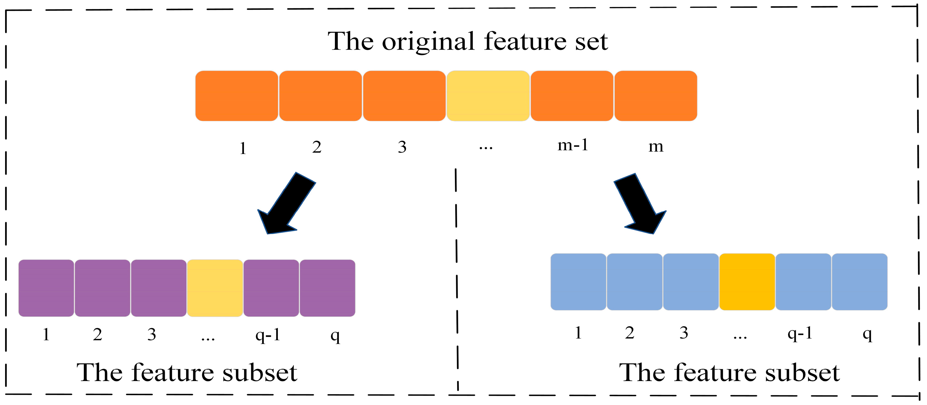
3.2.1. The Population Division Based on Feature Correlation

Generally, the population division involves partitioning the original feature set into multiple clusters (i.e., feature subsets) and initializing the agents generated in subpopulations based on these clusters. In addition, agents only search for features within their corresponding subsets while obtaining the rest via information interaction. Ideally, the population division considers the correlation between features or between features and labels commonly to minimize the correlation between features and maximize the correlation between features and labels [38]. However, when interactive features are partitioned into different subsets, subpopulations may fall into local traps that are not the local optimum of the original feature set and rather the local optimum resulting from the incorrect division. Therefore, the population division should ensure the feature subsets corresponding to subpopulations are sufficiently different, and the interactive features are partitioned together as much as possible, with the correlation between features considered.

Furthermore, generating many subsets requires an equal number of subpopulations to match them, leading to a large computation load. Additionally, interactive features may be divided into different subsets, resulting in mature convergence. To minimize the redundant features of the entire dataset, the population division decomposes the original feature set into two subsets, generating agents to form subpopulations within them. Figure 1 shows an example of the population division. The original feature set is partitioned according to the correlation between features, assuming that it has m features waiting for selection, two subsets are formed after the population division, and the number of features is $q.$ To maintain subpopulations’ balance, $q$ is equal to $⌊\mathrm{m}/2⌋$, the $\lfloor \rfloor$ is the integer-value function.

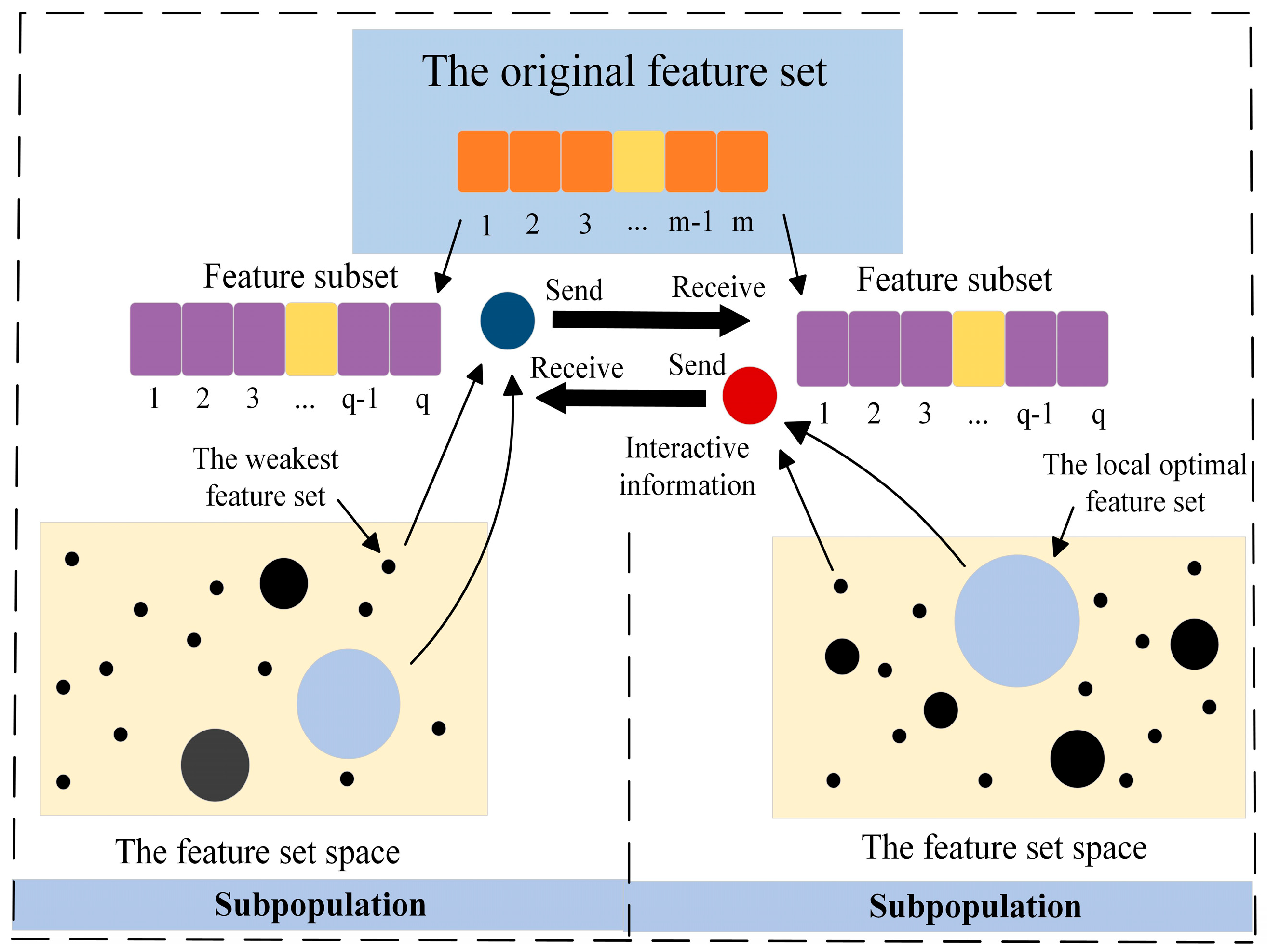
3.2.2. The Reliable Information Interaction

The agents in different subpopulations are designed to exchange the information in parallel to facilitate interaction. If a feature does not belong to the current feature subset, it is searched with a probability of 0. Moreover, subpopulations should be provided with representative information to keep balance. Features with unsatisfactory scores may be the result of not finding other interactive features [39]. With the representative information, the features’ performance will be boosted. The representative information is defined as the best and worst combinations searched by agents in the corresponding subpopulation, and one of them is selected as the interaction object to enhance the reliability of the co-evolution mechanism. Figure 2 illustrates the reliable information interaction between subpopulations. It can be seen that during the interaction, each subpopulation receives representative information from the other. The agent then combines this information to make an overall evaluation after conducting a search. By following this process, features will be fully searched to obtain a prominent classification accuracy through the support vector machine (SVM)-based classifier on the testing set.

In subpopulations, the position of the next iteration of agents (${\overrightarrow{X}}^{(iter+1)}$) is updated based on the distance ($\overrightarrow{d_{IS}}$) between the current agent’s position (${\overrightarrow{X}}^{iter}$) and the optimal position. Here, the positions of the current agents are updated based on the optimal agent obtained using Equation (5).

$${\overrightarrow{X}}^{(iter+1)}={\overrightarrow{X}}^{iter}-\overrightarrow{L}\cdot \overrightarrow{d_{IS}}$$

(5)

where $\overrightarrow{d_{IS}}$ refers to the distance between the current agent and the global optimum, while $\overrightarrow{L}$ denotes the social status of the optimum with a random value selected from the range of [−1, 1].

3.3. The Feature Recovering Mechanism

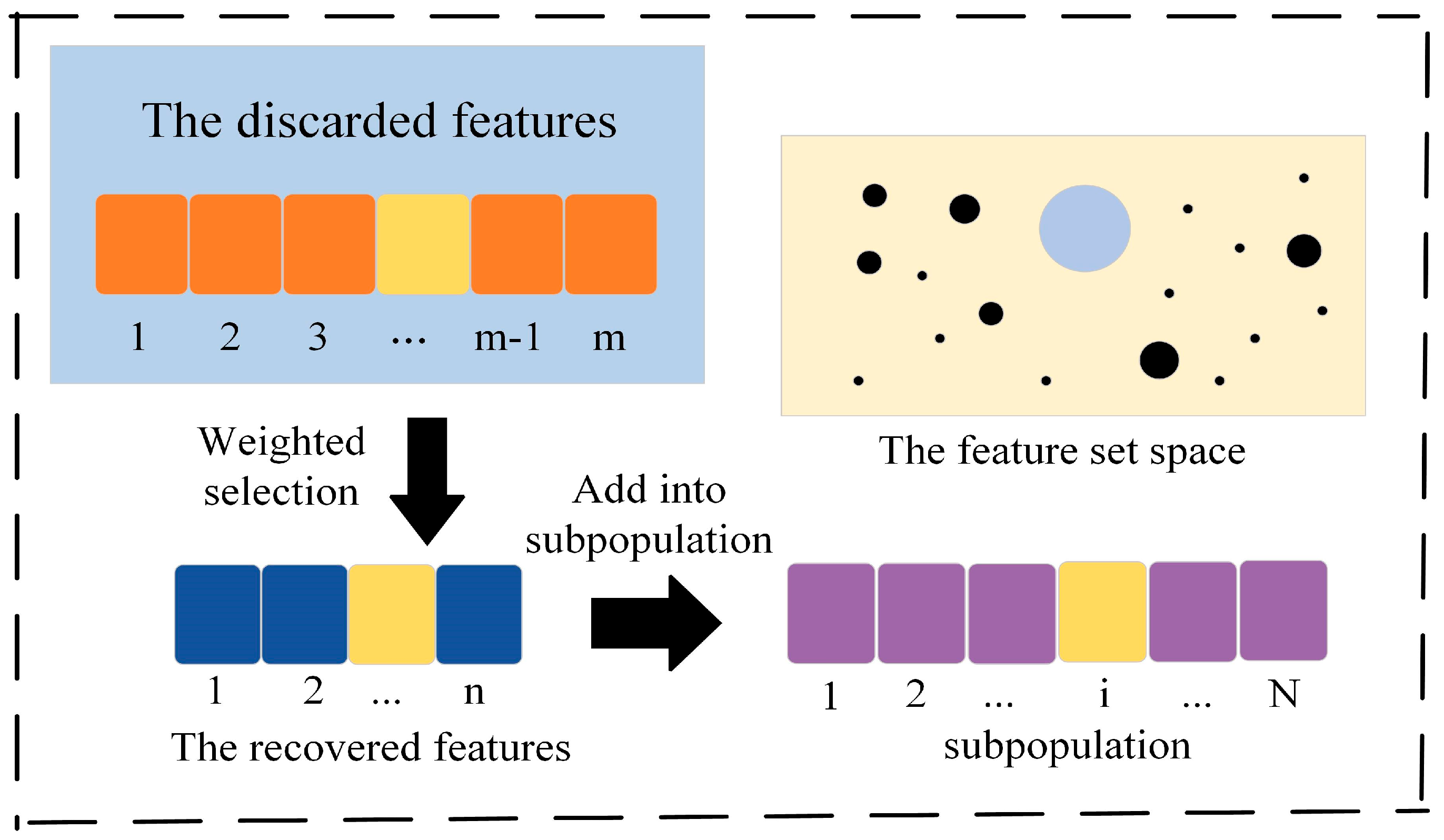
After the feature discarding, only the features with high ranking are selected, but the interactive features are not considered, which may lead to stagnation [40]. Consequently, the performance of feature subsets searched by agents may fall into local optima. Moreover, EA generally operates within the original feature set, and it is difficult to recycle the discarded features. To address these limitations, the feature recovering mechanism is applied to incorporate the recycled discarded features into the recovery subset, thereby increasing the probability of selection. The feature recovery mechanism has two stages. The first stage is reverse learning, which increases the probability of selecting features with low score ranking. Moreover, if training stagnation is detected, indicating that the subpopulation is not improved in successive iterations, some of the discarded features should be recycled. This will allow agents to fully search features later.

More attention should be paid to the features with low scores in the evaluative measures when recovering features. However, the low score does not necessarily mean that corresponding features should be simply discarded. Therefore, the lower-ranked features will receive higher weights. Assuming the dimension of input data is $m$, the calculation for weight is described below:

$$W^m=1-\frac{S^m}{{\sum }_{i=1}^m{S}_i^m}$$

(6)

where $W^m$ denotes the feature weight, and $S^m$ represents the feature score set obtained from feature discarding, $S_i^m$ represents the ith feature score. More weights obtained through Equation (6) are assigned to weak features, thus increasing their chances of being selected. As illustrated in Figure 3, after the features recovered through weighted screening are added to the corresponding subpopulation’s feature subset, a new feature space is generated for agents.

3.4. The Objective Function

The main target of feature selection is obtaining a representative feature combination from the original feature set to maximize the OA [41], which is an important evaluation criterion, but how to decrease the number of selected features is also a crucial target in feature selection. In this paper, the objective function is used to evaluate the feature combination searched by agents [42]; it is described in Equation (7).

$$fitness=\alpha \cdot OA+\left(1-\alpha \right)\cdot \lg \left(\frac{n_c}{n_s}\right)$$

(7)

where $fitness$ represents the fitness value of the feature combination searched by agents, $OA$ represents the overall classification accuracy obtained by SVM. Note that $n_{\mathrm{c}}$ and $n_{\mathrm{s}}$ are the number of total features in the dataset and the number of selected features. $\alpha$ is a weight factor of $OA$ and the number of selected features; it takes $\alpha$ = 0.9 in this paper.

3.5. Implementation of the Proposed Method

The proposed feature selection method updates the agent based on distance, and its key process involves the information interaction between agents. Moreover, in the event of stalling, it recycles some of the discarded features, thereby improving the probability of features with low score ranking. The proposed feature selection method is described as follows (Algorithm 1):

Algorithm 1: Discarding–recovering and co-evolution mechanisms for HSI feature selection

Input: the n $\times$ m dataset D, the agent size Agesize, the number of feature groups M by reverse learning, and the maximum number of iterations Maxiter Output: the effective feature combination selected by agents  Undergo the feature discarding process through the feature discarding mechanism and obtain the SS and DS using the Equations (1)–(4) by reverse learning M feature groups  for i in SS:  do   $W_i^m$ $\leftarrow$ $1-\frac{S_i^m}{{\sum }_{k=1}^m{\mathrm{S}}_k^m}$  end for The SS is divided into two subsets SS1 and SS2 based on the correlation  Selectgroup1 $\leftarrow$ SS1, Selectgroup2 $\leftarrow$ SS2  Two subpopulations are generated in Selectgroup1 and Selectgroup2 and Agesize agents are obtained  t $\leftarrow$ 0  while t < Maxiter:  do   Update the location of each agent by Equation (5) Update the fitness value of each agent by Equation (7)   if the optimal solution has been updated then    Exchange the information through interaction   end if   if one of the subpopulations has stalled then    h $\leftarrow$ Recover(subset)    SS $\leftarrow$ Add(SS, h), DS $\leftarrow$ Sub(DS, h), Selectgroup1,2 $\leftarrow$ Add (Selectgroup1,2, h),     S $\leftarrow$ Add(s, h)   end if   t $\leftarrow$ t + 1  end while  return The OA of effective feature combination

In the beginning, the feature evaluation is performed on all agents to discard the features with low score ranking, resulting in a selected set (SS) of features and a discarded set (DS) of features. The SS is then divided into two subsets: selectgroup₁ and selectgroup₂. Representative information is exchanged between these subsets when the optimal agent is updated. Moreover, if the stagnation phenomenon is detected, the feature recovering mechanism is triggered to recycle a recovery feature subset with a certain number based on the adaptive weight W. These features will be added to the SS and removed from the DS. The iteration process continues until the maximum iteration is reached.

4. Experimental Results

The proposed feature selection method is implemented using Python 3.8 on a personal computer that has a 2.30 GHz CPU, 8.00 GB RAM, and the Windows 8 operating system. To evaluate the performance of the proposed method, three HSI datasets, namely KSC (176 bands), Salinas (204 bands), and Longkou (270 bands), are used in the study. The experimental results are compared with some feature selection methods with EA-based, co-evolution mechanism-based, and others, and each independent experiment is performed in 30 operations with 50 iterations of each operation.

4.1. Dataset Description

The first dataset was acquired by NASA at the Kennedy Space Center (KSC) in Florida. It was obtained from a distance of approximately 20 km and contained 224 bands with a spatial resolution of 18 m. After removing bands with water absorbance and low signal-to-noise ratio, 176 bands were used for verification. The image consists of 512 $\times$ 614 pixels.

The second HSI dataset, named Salinas, was obtained by an AVIRIS sensor in the Salinas Valley of California, USA. It consists of 204 bands with a spatial resolution of 3.7 m and a pixel size of 512 $\times$ 217. The spectral range of the dataset spans from 0.4 to 2.5 μm, and the spectral resolution is 10 nanometers.

The third dataset was obtained in Longkou Town, Jingzhou City, Hubei Province, China, and includes six classes in an agrarian context. The UAV flew at an altitude of 500 m, and the spatial resolution of the airborne hyperspectral image is approximately 0.463 m. The image size is 550 $\times$ 400, with 270 bands ranging from 400 to 1000 nm.

The class names and corresponding sample numbers of three HSI datasets are described in

Table 1. The land-cover classes of three HSI datasets.

Class Number	Class Name	Sample Number	Class Name	Sample Number	Class Name	Sample Number
1	Scrub	761	Brocoli_green weeds_1	2009	Corn	34,511
2	Willow swamp	243	Brocoli_green weeds_2	3726	Cotton	8374
3	Cabbage palm Hammock	256	Fallow	1976	Sesame	3031
4	Cabbage palm/Oak hammock	252	Fallow_rough plow	1394	Broad-leaf soybean	63,212
5	Slash pine	161	Fallow_smooth	2678	Narrow-leaf soybean	4151
6	Oak/Broadleaaf hammock	229	Stubble	3959	Rice	11,854
7	Hardwood swamp	105	Celery	3579	Water	67,056
8	Graminoid marsh	431	Grapes_Untrained	11,271	Roads and houses	7124
9	Spartina marsh	520	Soil vineyard develop	6203	Mixed weed	5229
10	Cattaial marsh	404	Corn_senesced greed_weeds	3278	-	-
11	Salt marsh	419	Lettuce_romaine 4 wk	1068	-	-
12	Mud flats	503	Lettuce_romaine 5 wk	1927	-	-
13	Water	927	Lettuce_romaine 6 wk	916	-	-
14	-	-	Lettuce_romaine 7 wk	1070	-	-
15	-	-	Vinyard_untrained	7268	-	-
16	-	-	Vinyard_vertical_trellis	1087	-	-
-	Total	5211	Total	54,129	Total	204,542

. The image scene and ground truth of them are shown in Figure 4.

4.2. Parameters Setting of EAs

Before running, some parameters of EAs should be set for the heuristic search. The performance of the effective feature combination is dependent on the setting of parameters to some extent. In this paper, several EA-based feature selection methods, including PSO [43], FA [44], GWO [45], and GSA [46], are adopted to provide an intuitive performance comparison with the proposed method.

Table 2. Parameters setting of each algorithm.

Parameters	Values
Size of agents	15
Dimension	Number of features
The number of iterations per algorithm	50
The acceleration constant $c_1,c_2$ in PSO	2
Min-max inertia weight ${\omega }_{min}$, ${\omega }_{max}$ in PSO	0.2, 0.9
The light intensity absorption coefficient $I$ in FA	1
The step factor $\alpha$ in FA	0.97
Min-max attraction ${\beta }_{min}, {\beta }_{max}$ in FA	0.2, 1
$\mathsf{\alpha }$ Correlation coefficient in GWO	[2, 0]
The initial universal gravitational constant in GSA	100
Number of the subpopulation in co-evolution mechanism	2

shows the parameters setting by these EAs.

4.3. Experiments for the Search Ability

Table 3. The OA and Kappa coefficient of EA-based feature selection methods.

Datasets	Metrics	PSO	FA	GWO	GSA	Proposed
KSC	OA (%)	90.97 ± 0.33	90.26 ± 0.24	90.92 ± 0.31	90.71 ± 0.38	92.07 ± 0.12
	Kappa	0.904 ± 0.002	0.887 ± 0.0016	0.897 ± 0.001	0.892 ± 0.002	0.917 ± 0.001
	WTL	+	−	+	+	28/0/2
Salinas	OA (%)	91.77 ± 0.15	91.63 ± 0.23	91.65 ± 0.17	91.82 $\pm$0.26	92.36 ± 0.21
	Kappa	0.907 ± 0.001	0.908 ± 0.0014	0.905 ± 0.001	0.909 ± 0.0018	0.915 ± 0.0013
	WTL	+	−	+	−	27/1/2
Longkou	OA (%)	97.36 $\pm$0.11	96.89 ± 0.27	97.12 ± 0.41	97.74 ± 0.33	98.01 ± 0.14
	Kappa	0.964 $\pm$0.0002	0.956 ± 0.001	0.960 ± 0.0024	0.969 ± 0.006	0.979 ± 0.002
	WTL	+	−	+	+	30/0/0

presents the OA and Kappa coefficient after 30 independent operations, while WTL is the win/tie/loss indicator of the fitness value.

Table 4. Number of selected features and CPU time of EA-based feature selection methods.

Datasets	Metrics	PSO	FA	GWO	GSA	Proposed
KSC	Num	49.6	50.3	50.7	55.3	42.2
	Time	190.1176	152.4127	204.1769	195.3568	150.6149
Salinas	Num	67.5	55.3	56.7	55.6	43.1
	Time	3600.5043	2714.3658	3536.9347	3742.5928	2427.6280
Longkou	Num	95.7	68.7	76	95.4	62.5
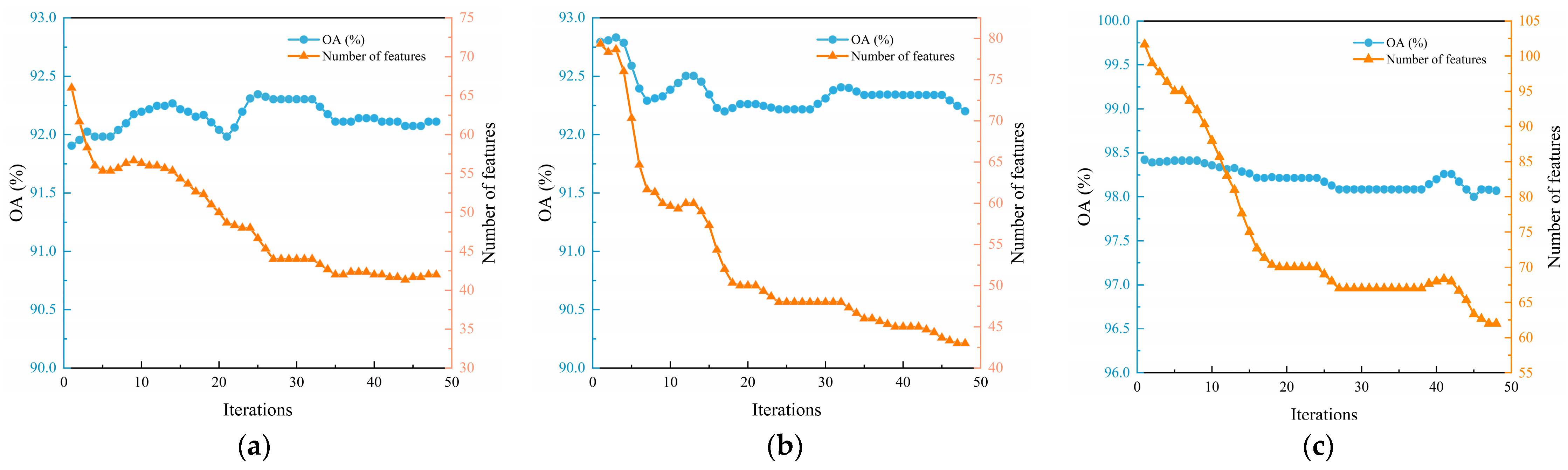
	Time	1564.3620	1269.3795	1514.6489	1892.3481	1204.7301

shows the number of features (Num) and CPU time (Time) selected by the 30 independent operations. To demonstrate the prominent OA of the effective feature combination achieved in each iteration, the average number of features and OA are obtained for each iteration, as shown in Figure 5, and the fitness value is shown in Figure 6.

According to Table 3, the proposed method outperforms PSO, FA, GWO, and GSA in search capability, which achieves a prominent OA, surpassing PSO, FA, GWO, and GSA by 1.1%, 1.81%, 1.15%, and 1.36%, respectively. Those experimental results exhibit the superior searchability of the proposed method. Moreover, it enhances the development potential of local search by using a feature recovery mechanism. Its winning frequency is higher than 27, especially in Longkou, where it reached 30. These demonstrate the prominent stability of the proposed method and the superior exploration ability.

According to Table 4, the proposed method exhibits significantly higher reductive efficiency than other EA-based feature selection methods. Specifically, it selects less than 20% of the features from the HSI dataset, resulting in the selection of only 42 features out of a total of 176 bands in the KSC dataset while achieving a prominent OA. The Salinas dataset, it selects approximately half number of features compared with GSA yet achieves a better OA. On average, other methods select 58.7 features, whereas the proposed method selects only 43.1 features, indicating superior performance. In addition, the feature discarding mechanism substantially reduces redundant features, thereby shrinking the feature space and improving the computation time, especially in the Longkou dataset.

As shown in Figure 5, after feature discarding, the number of selected features searched by agents is still high, and the number of features is decreased after the heuristic search, while the OA is little to no fluctuation, demonstrating the prominent stability of the proposed method. Furthermore, the feature recovering mechanism effectively updates agents before the iteration ends, indicating that the proposed feature selection method possesses a prominent ability to escape from local optima. According to Figure 6, the fitness value is visualized to comprehensively evaluate the searching ability of each algorithm, and the proposed feature selection method achieves promising results on three HSI datasets and ranks 1^st in terms of average fitness value, followed by GWO, FA, PSO, and GSA. Moreover, the proposed method achieves the optimal fitness value on three HSI datasets compared with other EA-based methods, proving it has a prominent search ability for feature selection.

4.4. Comparison with Other Feature Selection Methods

To assess the impact on each class, some feature selection methods in HSI datasets are compared in the experiment: maximum information minimum redundancy (MRMR) [47], joint mutual information with class correlation (JOMIC) [48], joint mutual information maximization (JMIM) [49], conditional mutual information maximization (CMIM) [50] and shallow-to-deep feature enhancement (SDFE) [51]. The experiments are performed on 10% to 25% of the total features. The accuracy for each class and Kappa coefficient are shown in

Table 5. The results for the KSC dataset using 10% of the total number of features.

Class Number	MRMR	JOMIC	JMIM	CMIM	SDFE	Proposed
1	92.5714	86.6579	88.4363	81.4724	92.3717	92.4264
2	86.2559	86.2222	93.2990	86.7841	86.1751	89.3519
3	63.4675	69.9670	74.7170	83.8542	85.4077	77.4074
4	52.9070	60.1990	52.1886	51.9231	55.5556	57.7670
5	62.5000	73.1183	75.0000	70.3704	68.3761	65.0407
6	60.8434	60.9929	70.4918	64.8936	83.4711	71.0059
7	67.9487	78.4091	71.4286	83.3333	74.7826	74.0741
8	76.5661	79.4304	76.7442	68.6981	87.6238	93.9058
9	82.6430	86.4341	84.4530	90.9692	90.2390	89.9606
10	87.6081	100.0000	100.0000	99.1562	99.8727	99.9618
11	95.5959	95.4054	98.8950	99.1892	98.5836	93.6869
12	91.3551	79.9213	76.8642	74.0876	92.7039	97.9499
13	99.5175	99.9482	99.2894	99.8801	99.6247	99.9915
OA (%)	85.0320	86.0128	85.7143	84.5203	90.2132	90.3624
Kappa	0.8406	0.8543	0.8418	0.8370	0.8908	0.8917

,

Table 6. The results for the KSC dataset using 15% of the total number of features.

Class Number	MRMR	JOMIC	JMIM	CMIM	SDFE	Proposed
1	91.8733	92.5104	88.2108	88.9655	92.8870	92.2006
2	89.6226	90.4762	72.0755	82.0961	88.7324	90.6977
3	70.7071	69.2557	77.7328	84.6154	80.2469	83.4711
4	48.4733	56.6845	56.7742	58.2996	57.9336	60.2996
5	82.0513	79.4872	73.3333	52.9032	75.2381	86.6667
6	78.4314	66.6567	71.5789	66.6667	65.1007	73.6842
7	70.1923	73.4513	81.5789	72.4771	74.2268	70.5357
8	80.9645	87.7612	85.0785	72.2343	89.5408	88.5856
9	82.7778	78.1570	87.1401	89.1304	91.6667	89.9408
10	87.8873	91.9162	100.0000	100.0000	99.7183	96.8927
11	98.3562	96.3824	98.4000	99.4350	97.6378	95.1157
12	92.9440	93.7811	94.4056	93.1925	98.1352	97.6526
13	98.4597	98.1065	99.9919	66.6667	100.0000	100.0000
OA (%)	86.5885	87.0362	87.9104	87.0362	90.5970	90.6397
Kappa	0.8514	0.8560	0.8644	0.8581	0.8925	0.8936

,

Table 7. The results for the KSC dataset using 20% of the total number of features.

Class Number	MRMR	JOMIC	JMIM	CMIM	SDFE	Proposed
1	92.9178	90.7609	87.2679	86.2924	92.0833	93.1642
2	91.7476	86.1472	88.8889	88.4793	95.5801	88.5416
3	73.6462	72.5632	85.8537	90.7407	85.7759	79.4165
4	60.5634	48.8189	56.2500	59.3156	58.0000	68.2564
5	65.9091	79.6875	72.7273	58.2677	78.5047	78.2196
6	65.1613	77.0833	69.3548	67.7419	78.8618	72.2519
7	77.1429	80.6818	74.5763	72.0339	92.0930	85.6429
8	82.9268	88.8298	81.7043	82.4818	86.8106	93.4579
9	88.5177	88.2828	88.3268	88.7574	92.6295	90.1245
10	91.3793	92.6686	99.9948	99.4444	97.7077	99.9094
11	97.6501	95.3728	99.9859	98.1283	98.9333	99.9654
12	92.2902	92.4242	95.7143	97.2772	97.3872	95.6413
13	99.6407	99.7599	100.0000	99.9618	100.0000	100.0000
OA (%)	88.3156	88.2942	88.7846	88.8699	90.9595	91.7057
Kappa	0.8712	0.8628	0.8750	0.8735	0.8992	0.9047

,

Table 8. The results for the KSC dataset using 25% of the total number of features.

Class Number	MRMR	JOMIC	JMIM	CMIM	SDFE	Proposed
1	94.5428	93.5897	90.2878	89.9015	91.5395	94.2413
2	89.6714	91.9431	86.5169	92.3729	88.5572	98.5618
3	69.4444	73.6301	77.7778	88.0000	87.1111	87.1594
4	56.3636	54.1176	60.3960	60.5442	61.9910	69.5432
5	83.3333	85.5072	75.0000	72.7273	75.8929	84.5621
6	62.4309	73.4463	71.4286	68.2353	68.0203	77.8654
7	69.5238	78.2178	91.0448	79.3103	75.2137	72.5613
8	86.9674	91.1111	82.1306	83.3333	90.0990	93.6421
9	88.1764	88.5375	88.0299	95.1807	92.0892	92.6578
10	98.8338	94.9861	100.0000	99.9185	99.7175	99.9153
11	97.9058	98.5836	99.9103	97.1963	97.7901	97.2541
12	97.5717	94.0552	90.5983	92.6923	97.5501	98.4623
13	99.9826	99.5910	99.8459	100.0000	100.0000	99.8917
OA (%)	89.4883	89.8507	89.1721	90.3300	91.1514	92.8144
Kappa	0.8742	0.8819	0.8893	0.8991	0.9014	0.9164

,

Table 9. The results for the Salinas dataset using 10% of the total number of features.

Class Number	MRMR	JOMIC	JMIM	CMIM	SDFE	Proposed
1	99.5343	98.8636	100.0000	100.0000	99.8862	99.9654
2	97.2044	98.1765	97.9009	98.0724	98.5891	98.1319
3	92.7253	94.6309	89.8361	92.1729	94.4625	91.2998
4	98.0614	97.9032	99.1948	97.9592	97.1919	98.8606
5	97.8351	98.0897	95.3859	92.2832	98.4127	99.1625
6	99.4410	99.9438	99.3292	99.6081	99.7199	99.9438
7	97.7411	97.6190	99.9373	98.9480	99.0081	99.4410
8	74.1664	73.8863	70.0681	71.0198	74.8498	74.2189
9	97.9937	98.0613	96.5974	93.7715	99.1081	98.1501
10	94.0709	90.5249	86.0244	87.9890	94.5692	92.3497
11	94.6352	97.6852	76.1431	73.6961	95.5032	87.8981
12	91.0464	93.7778	93.0586	93.3839	95.7589	96.8362
13	93.1193	96.4200	90.2004	93.3180	93.7500	94.8598
14	98.6957	98.7179	95.7356	98.4305	98.0088	98.4749
15	77.0670	78.4153	77.4679	75.3187	80.4813	91.4327
16	98.5255	98.8032	99.6269	99.5019	99.6193	99.7484
OA (%)	89.3674	89.5685	87.3106	87.2573	90.4799	90.1081
Kappa	0.8797	0.8816	0.8657	0.8659	0.8936	0.8905

,

Table 10. The results for the Salinas dataset using 15% of the total number of features.

Class Number	MRMR	JOMIC	JMIM	CMIM	SDFE	Proposed
1	99.1982	99.9989	100.0000	100.0000	99.7517	100.0000
2	97.8947	98.2456	98.5832	98.3510	99.3765	99.5247
3	93.9427	91.5418	90.2646	94.9324	93.1071	94.8578
4	94.4870	97.7707	98.7302	97.5000	97.9528	99.0476
5	98.1387	97.6840	97.7215	97.1193	98.8215	98.1148
6	99.9987	100.0000	99.9438	99.9846	99.9438	100.0000
7	98.3446	99.0087	99.8118	99.0093	99.3808	99.2560
8	74.3518	74.5124	75.0246	75.4254	76.8367	78.0508
9	99.1783	99.0046	96.3605	97.5506	99.3585	99.2479
10	91.3971	93.1818	86.8185	86.8385	93.8272	95.9028
11	92.8421	97.1111	87.4157	87.6518	96.9365	96.0526
12	92.8414	94.9381	96.9629	96.4206	95.7589	96.2963
13	94.6262	96.1814	90.8072	92.8899	98.0583	94.6009
14	98.9035	98.2684	97.3154	96.3907	96.9199	94.6030
15	77.8520	78.5059	82.9680	82.0026	78.9930	81.5315
16	99.0826	98.9717	98.5258	99.5031	99.4987	99.0111
OA (%)	89.6342	90.0324	89.7656	90.0283	91.0142	91.7074
Kappa	0.8825	0.8876	0.8815	0.8936	0.9013	0.9105

,

Table 11. The results for the Salinas dataset using 20% of the total number of features.

Class Number	MRMR	JOMIC	JMIM	CMIM	SDFE	Proposed
1	99.4420	99.7738	100.0000	99.9843	99.4562	99.9913
2	99.4069	98.8797	98.9399	99.5258	98.9399	99.5848
3	95.0166	94.3844	92.3409	91.9181	94.1748	94.8408
4	97.3101	95.8333	97.8056	98.4227	99.3620	98.1132
5	98.5062	98.8235	98.3165	97.3177	97.9525	99.2437
6	100.0000	99.7205	99.9437	99.9439	99.8426	99.9439
7	99.4420	99.2551	99.9958	100.0000	99.6278	99.4406
8	75.6456	74.8615	75.5213	75.4221	78.1847	78.7730
9	98.6116	98.9015	97.1339	98.2715	99.2855	99.4298
10	93.5461	94.0072	88.2393	91.5014	96.0114	97.5300
11	91.0537	94.7253	91.1700	85.3061	95.2174	93.8819
12	95.3933	95.2009	97.0688	95.9866	96.8433	95.2486
13	95.2381	94.1452	95.0588	95.0588	96.6746	97.8208
14	97.2574	98.4881	98.0728	97.0402	96.5092	98.3368
15	77.3140	79.7858	83.1199	83.0685	78.8020	83.4154
16	98.3668	98.0964	99.3797	99.2583	97.4421	99.3750
OA (%)	90.3198	90.3321	90.3937	90.4347	91.3294	92.2411
Kappa	0.8907	0.8925	0.8901	0.8968	0.9047	0.9200

,

Table 12. The results for the Salinas dataset using 25% of the total number of features.

Class Number	MRMR	JOMIC	JMIM	CMIM	SDFE	Proposed
1	99.7743	99.4388	100.0000	99.9846	100.0000	100.0000
2	98.9971	99.1124	98.6382	98.4174	98.9393	99.8322
3	96.5324	96.8750	91.7559	92.9638	93.9297	96.1354
4	97.4724	97.9528	99.0461	98.4202	98.8906	99.3782
5	97.9305	99.0033	97.0906	98.5012	99.6619	99.5342
6	100.0000	99.9439	99.9438	99.8315	99.9438	99.9473
7	99.3180	99.4389	98.9467	99.7492	99.5644	99.9544
8	77.0343	75.3308	76.4241	75.4392	77.2064	80.7261
9	98.9362	99.0747	98.0524	97.1100	99.4294	99.4388
10	92.7785	93.4540	91.5855	93.6324	98.3138	97.7492
11	93.9759	96.4835	92.4406	92.7602	95.5789	98.9252
12	95.8567	95.8520	94.9283	96.0894	96.4126	98.7631
13	93.1034	95.6627	94.7743	96.8750	97.1429	99.3150
14	98.6813	95.8763	95.3586	97.3029	97.2973	98.5960
15	76.6654	80.1782	84.4185	84.4747	82.6695	84.2496
16	98.6076	98.2478	99.6264	99.5037	98.4029	99.5761
OA (%)	90.6893	90.7098	90.7960	90.7591	91.7607	93.2614
Kappa	0.8845	0.8914	0.8946	0.8935	0.9079	0.9251

,

Table 13. The results for the Longkou dataset using 10% of the total number of features.

Class Number	MRMR	JOMIC	JMIM	CMIM	SDFE	Proposed
1	96.3905	98.3974	73.6477	72.1819	98.6880	98.0647
2	88.8722	80.9339	38.6952	56.6265	86.0244	89.4598
3	95.2000	96.5035	0.0000	0.0000	96.8468	90.7834
4	94.9534	95.8103	72.4373	73.0363	97.4190	96.8578
5	74.8555	79.7403	0.0000	16.6667	75.0000	83.3333
6	95.7386	93.5909	0.0000	0.0000	93.8721	95.0276
7	99.9834	99.9834	84.6953	85.1456	100.0000	100.0000
8	87.3580	92.5262	0.0000	48.6330	91.6667	94.0458
9	70.6941	74.0634	38.3442	36.0714	86.9010	90.5724
OA (%)	95.4965	95.9963	72.9248	74.4785	96.9090	97.1208
Kappa	0.9731	0.9733	0.6845	0.7055	0.9793	0.9815

,

Table 14. The results for the Longkou dataset using 15% of the total number of features.

Class Number	MRMR	JOMIC	JMIM	CMIM	SDFE	Proposed
1	97.7496	97.6906	73.8964	74.6577	99.2295	99.3867
2	90.7609	91.1444	38.6128	58.0488	82.5495	89.7638
3	95.4802	98.8571	0.0000	0.0000	96.5665	95.7219
4	95.8955	96.1853	73.4588	75.8225	97.8005	96.4383
5	82.0442	81.6216	0.0000	25.0000	86.4407	85.7520
6	94.1784	93.5574	0.0000	0.0000	95.3447	96.2829
7	99.9834	99.9834	85.3745	87.0789	99.9503	99.9834
8	90.0000	90.3226	100.0000	50.1294	92.2272	94.4109
9	84.7458	83.3333	41.9118	38.4615	94.6844	93.0818
OA (%)	96.5721	96.6319	73.5984	76.5754	97.4413	97.4522
Kappa	0.9552	0.9560	0.6456	0.7110	0.9863	0.9867

,

Table 15. The results for the Longkou dataset using 20% of the total number of features.

Class Number	MRMR	JOMIC	JMIM	CMIM	SDFE	Proposed
1	96.3905	98.4955	86.5508	89.1432	98.8821	99.2585
2	88.8722	89.0357	56.8080	55.0672	85.9626	88.7850
3	95.2000	96.9231	0.0000	0.0000	99.9917	94.2731
4	94.9534	96.1932	83.9454	86.5783	97.4028	98.1774
5	74.8555	80.6283	3.8462	0.0000	82.4289	84.6753
6	95.7386	96.1825	0.0000	0.0000	96.3470	95.0673
7	99.9834	99.9834	92.4528	90.3115	99.9503	100.0000
8	87.3580	90.1306	60.3004	55.6107	93.2635	93.8160
9	70.6941	90.9091	73.4375	96.5217	95.3642	96.2865
OA (%)	95.4965	96.9035	84.5719	85.2890	97.4957	97.8596
Kappa	0.9731	0.9767	0.8060	0.8114	0.9849	0.9894

and

Table 16. The results for the Longkou dataset using 25% of the total number of features.

Class Number	MRMR	JOMIC	JMIM	CMIM	SDFE	Proposed
1	99.4819	99.3237	91.1993	90.2739	99.6143	99.1987
2	92.2865	87.6963	60.2791	60.7280	87.4667	87.3533
3	97.8723	99.4382	99.2701	97.7778	99.0868	97.7376
4	96.0814	96.7295	94.9780	95.6297	97.3448	98.3615
5	81.3602	79.3367	31.2500	14.0351	83.3333	86.5169
6	96.4674	96.3504	85.2273	69.6970	96.0253	97.7860
7	99.9669	99.9668	87.4238	87.3244	99.9669	99.9503
8	92.5150	92.3767	83.2187	83.4019	92.5595	91.8999
9	92.1311	86.7069	89.6970	78.4504	92.9012	97.5430
OA (%)	97.3055	97.1480	88.8309	88.3909	97.5771	98.0389
Kappa	0.9715	0.9852	0.8583	0.8535	0.9880	0.9910

.

4.4.1. The Result of the KSC Dataset

Table 5, Table 6, Table 7 and Table 8 show the OA and Kappa coefficients for the KSC dataset using 10–25% of the total number of features.

Based on Table 5, Table 6, Table 7 and Table 8, it is concluded that the proposed feature selection method outperforms MRMR, JOMIC, JMIM, CMIM, and SDFE in terms of the OA for different numbers of features, with an improvement of over 0.7%. Furthermore, when using 20% of the total number of features, the Kappa coefficient reaches 0.9, demonstrating that its OA is basically anastomotic with the labels. For 25% of the total number of features, other feature selection methods have an OA of below 91.2%, while the proposed method achieves the OA and Kappa coefficients exceeding 92.8% and 0.916, respectively. Moreover, the proposed method takes the OA of over 97% for five classes, with Willow swamp, Cattaial marsh, and Mudflats even reaching 98%. In summary, it is a practical feature selection method for the KSC dataset.

4.4.2. The Result of the Salinas dataset

Table 9, Table 10, Table 11 and Table 12 present the OA and Kappa coefficients for the Salinas datasets using a fixed number of features.

The experimental results demonstrate that the proposed method outperforms other commonly used feature selection methods, achieving an OA of over 92% while obtaining the total number of features by less than 20%. Moreover, the Kappa coefficient for 25% of the total number of features is 0.2 higher than that of other methods, and the OA is higher for each class, with an OA of over 96% for all 14 classes. Notably, the samples of Brocoli_green_beads_1 are all correctly identified. These indicate that it achieves a prominent OA and Kappa coefficient for each class of the Salinas datasets, demonstrating the superiority of the proposed method.

4.4.3. The Result of the Longkou Dataset

Table 13, Table 14, Table 15 and Table 16 present the OA and Kappa coefficients for the Longkou datasets using a fixed number of features.

Table 13, Table 14, Table 15 and Table 16 present the OA and Kappa coefficients in the Longkou dataset. It is evident that the proposed method obtains prominent OA and Kappa coefficients, and it maintains a clear advantage in the classification of a small number of features. In the experimental comparison using 10% of the total number of features, MRMR, JOMIC, and SDFE achieve an OA of below 97%, while the proposed method achieves an OA of as high as 97.1%, which is 1.6%, 1.1% and 0.2% higher than MRMR, JOMIC, and SDFE, respectively. The OA of JMIM and CMIM is lower than 89%. The Kappa coefficient also demonstrates an overall advantage for the proposed method. Those results indicate that it is a robust and feasible feature selection method for the Longkou dataset.

5. Discussion

5.1. Design Analysis of the Proposed Method

EA is an effective strategy to obtain a feature combination of HSI datasets with a preferable OA in a limited time, the OA obtained on three HSI datasets exceeds 90%, and some even reach 98%. However, it is prone to stagnation during iteration due to the insufficient interactivity of agents. Co-evolution is a prominent mechanism to improve the agents’ diversity, the original feature set is divided into some subsets, and agents are generated by those to form subpopulations. Moreover, information interaction exchanges the optimal feature combination searched by agents to maintain the balance of subpopulations, but solely exchanging the optimal feature combination reduces the selected probability of interactive features. The proposed method incorporates reliable information interaction and a series of mechanisms focusing on features to address this. The trajectory of the OA for each iteration indicates that the stability of the proposed method, is decreased by less than 0.5% as the feature space condenses, and the computational time is also reduced by an average of 15%.

The proposed method has a prominent OA in most of the classes and even reaches 100% for Brocoli_green_beads_1 in the KSC dataset and Water in the Longkou dataset. Although it is lower than other feature selection methods in a few classes, the difference is not apparent in the class with small samples. Although other methods based on measure criteria stand out in terms of efficiency, it is difficult to distinguish interactive features as the number of instances increases. Feature discarding is an effective mechanism for eliminating redundant information and improving the computational load. Similar to other feature selection methods, the OA is negatively impacted due to improper discarding. To counterbalance this effect, the feature recovering mechanism is employed to improve the generalization ability while maintaining the OA at a high level. Experimental results indicate that the OA of the proposed method surpasses other feature selection methods by an average of 3%, and important features are adequately restored by the feature recovery mechanism, thereby improving the performance and reliability of the proposed method.

5.2. Discussion for the Training Size

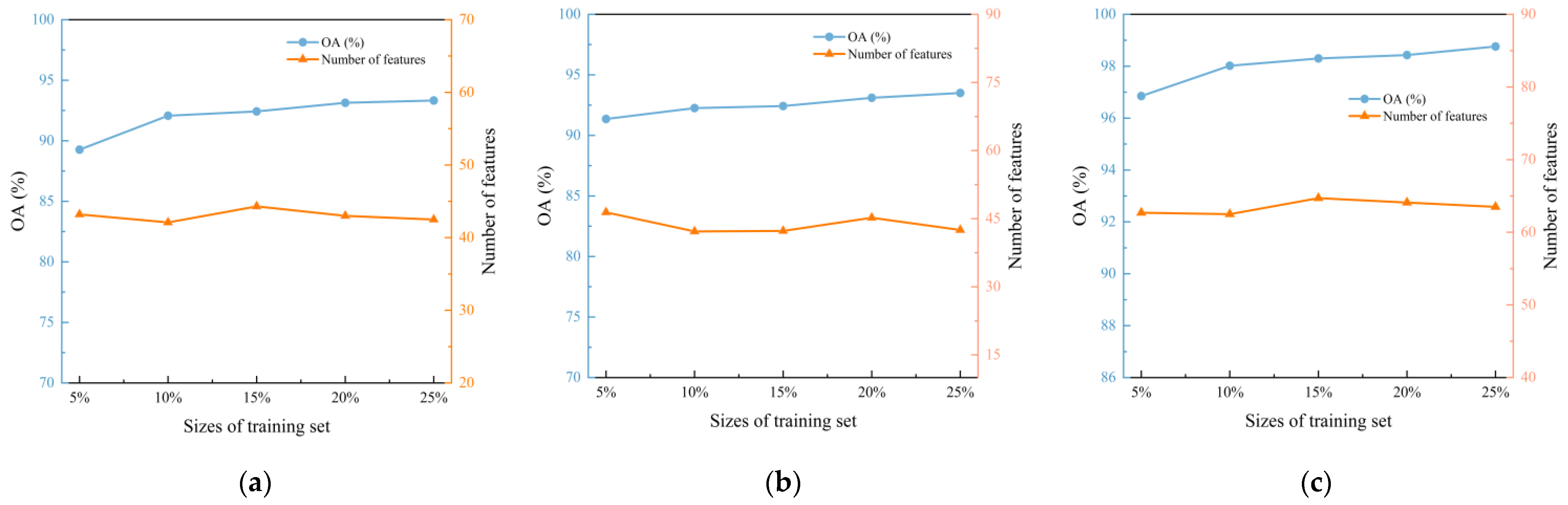
In Section 4.1, three HSI datasets, namely, KSC, Salinas, and Longkou, are introduced to validate the performance of the proposed method. The OA of effective feature combination and computation time is influenced by the size of the training set. Several tests are conducted on the proportion of the training set, ranging from 5% to 25%, because of the small-sample learning properties to determine the appropriate size of the training set. The change curves for the number of features and the OA of different training sets are shown in Figure 7.

The experimental results indicate that the increasing size of the training set from 5% to 10% leads to a significant improvement in the OA. However, further increasing the proportion from 10% to 25% only results in a minimal increase, while the computation time also decreases to some extent. Additionally, the number of selected features does not show significant fluctuations, so the size of the training set is designated as 10%. This size strikes a balance between the OA and computational load, making it a practical and effective choice for feature selection in HSI datasets.

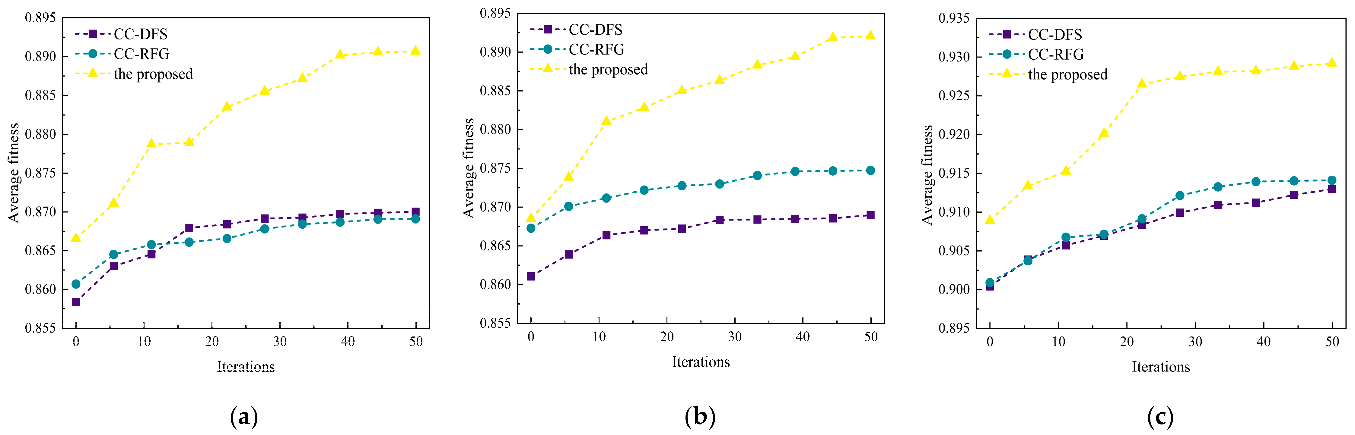
5.3. Comparison with Other Co-Evolution Mechanisms

To verify the search efficiency of the co-evolution mechanism in the proposed method, it is compared with other co-evolution mechanisms named CC-DFS [33] and CC-RFG [34]; the average fitness value of each iteration on three HSI datasets is shown in Figure 8.

In the beginning, the fitness value of the proposed method is higher than that of CC-DFS and CC-RFG in three HSI datasets, which demonstrates that the feature discard mechanism effectively removes the redundant features. With further iterations, the fitness trajectory of CC-DFS and CC-RFG gradually stabilizes while that of the proposed method remains upward. This indicates that the co-evolution mechanism enhances the search efficiency of agents and suggests a prominent ability to escape from local optima. As a result, the reliable co-evolution mechanism effectively interacts with more representative information, largely avoiding the occurrence of stagnation.

6. Conclusions

A feature selection method based on discarding–recovering and co-evolution mechanisms is proposed in this study with the aim of obtaining effective feature combinations in HSI datasets. According to the experimental results, the proposed method outperforms other EA-based feature selection methods, including PSO, FA, GWO, and GSA, in terms of optimization ability and search speed in the feature space. It achieves a prominent OA with a small number of selected features, outperforming other feature selection methods in this regard, and exhibits satisfied stability. In addition, through comparing with the other co-evolution mechanism, the fitness trajectory exhibits that the reliable co-evolution mechanism could interact with more representative information between agents, making them continuously improve. The performance limitations caused by feature discarding are improved through the recovery of dropped features, which guarantees the generalization ability and decreases computational load.

Furthermore, the proposed method outperforms MRMR, JOMIC, JMIM, CMIM, and SDFE in terms of the OA with varying numbers of features, and the reliable information interaction ensures a more balanced learning process, which maintains a positive balance between classification accuracy and the number of selected features, making it become a suitable choice for feature selection. In future studies, more representative criteria will be synthesized in the information interaction to further improve the diversity of agents. Moreover, it is interesting to use feature clustering to take the population division and further avoid population imbalance.