

Ship Target Detection in Optical Remote Sensing Images Based on E2YOLOX-VFL

1
School of Electronic Information Engineering, Nanjing University of Aeronautics and Astronautics, Nanjing 211106, China
2
Satellite General Department, Shanghai Institute of Satellite Engineering, Shanghai 201109, China
*
Author to whom correspondence should be addressed.
Remote Sens. 2024, 16(2), 340; https://0-doi-org.brum.beds.ac.uk/10.3390/rs16020340
Submission received: 18 November 2023
/
Revised: 31 December 2023
/
Accepted: 9 January 2024
/
Published: 15 January 2024
(This article belongs to the Special Issue Artificial Intelligence-Driven Methods for Remote Sensing Target and Object Detection II)
Abstract
:In this research, E2YOLOX-VFL is proposed as a novel approach to address the challenges of optical image multi-scale ship detection and recognition in complex maritime and land backgrounds. Firstly, the typical anchor-free network YOLOX is utilized as the baseline network for ship detection. Secondly, the Efficient Channel Attention module is incorporated into the YOLOX Backbone network to enhance the model’s capability to extract information from objects of different scales, such as large, medium, and small, thus improving ship detection performance in complex backgrounds. Thirdly, we propose the Efficient Force-IoU (EFIoU) Loss function as a replacement for the Intersection over Union (IoU) Loss, addressing the issue whereby IoU Loss only considers the intersection and union between the ground truth boxes and the predicted boxes, without taking into account the size and position of targets. This also considers the disadvantageous effects of low-quality samples, resulting in inaccuracies in measuring target similarity, and improves the regression performance of the algorithm. Fourthly, the confidence loss function is improved. Specifically, Varifocal Loss is employed instead of CE Loss, effectively handling the positive and negative sample imbalance, challenging samples, and class imbalance, enhancing the overall detection performance of the model. Then, we propose Balanced Gaussian NMS (BG-NMS) to solve the problem of missed detection caused by the occlusion of dense targets. Finally, the E2YOLOX-VFL algorithm is tested on the HRSC2016 dataset, achieving a 9.28% improvement in mAP compared to the baseline YOLOX algorithm. Moreover, the detection performance using BG-NMS is also analyzed, and the experimental results validate the effectiveness of the E2YOLOX-VFL algorithm.
1. Introduction
Remote sensing images are obtained by sensors carried by satellites, aircraft, and other platforms, allowing for observation of the Earth’s surface. One notable characteristic is their ability to capture large-scale data in a short period of time. Remote sensing images typically include information about objects such as rivers, farmland, forests, roads, cars, airplanes, and ships. Utilizing remote sensing images for object detection is an important application area. Ships hold significant importance, as they are crucial targets at sea, and automated ship detection and recognition play a vital role in gaining maritime control. Therefore, in-depth research on ship detection and recognition is essential.
Currently, remote sensing images employed for ship detection include Synthetic Aperture Radar (SAR) images, visual images, infrared images, and hyperspectral images. Among these, SAR and visual images are the most widely employed. Although SAR has the advantage of being able to see through clouds, SAR images lack visual intuitiveness and cannot provide detailed information such as ship material attributes [1,2,3]. Visual images obtained through optical remote-sensing technology offer a more realistic representation of color information of targets and backgrounds. They exhibit prominent structural features, making them unmatched in the domain of ship detection and classification in maritime regions compared to other image sources [4].
The detection and classification of ship targets in optical remote sensing images can be categorized into conventional approaches and deep learning-based techniques.
- 1.
- Conventional detection approaches often involve multiple steps and have limited accuracy. For instance, in [5], ship detection is achieved using image edge intensity, which is effective in distinguishing between ships and nonships and obtains a 95% detection accuracy. He et al. [6] utilized texture fractal dimension and gap features for ship detection. This method effectively eliminates the impact of sea clutter on the detection results, achieving good detection results under different signal-to-noise ratios. Furthermore, it is not affected by occlusion and rotation of moving targets, demonstrating better robustness compared to traditional methods based on target shape and point-line structures. In [7], utilizing the differences in multi-scale fractal features between ship targets and background images, the interference of sea and sky backgrounds on ship detection has been effectively eliminated. The experimental results demonstrate that this method can accurately and effectively detect targets, with a 97.1% detection rate and a 9.5% false alarm rate. Li et al. [8] used an image-based maritime ship detection method based on fuzzy theory, effectively eliminating false targets and efficiently and accurately detecting ship targets in images. Its Figure of Merit (FoM) is 25% higher than the CFAR algorithm. Zhao et al. [9] proposed a ship detection method combining multi-scale visual saliency, capable of successfully detecting ships of different sizes and orientations while overcoming interference from complex backgrounds. This method achieved a detection rate of 93% and a false alarm rate of 4%. Wang et al. [10] employed maximum symmetric surround saliency detection for initial candidate region extraction and combined ship target geometric features for candidate region pre-filtering, achieving ship detection even in complex sea backgrounds. The detection accuracy is 97.2%, and the detection performance is better than most ship detection algorithms. Though these methods make use of the strong perception ability of the human visual system for nearby objects, they face challenges in selecting salient features due to factors such as atmospheric conditions, marine environments, and imaging performance.
- 2.
- In contrast, deep learning methods have gained considerable momentum due to their advantage in extracting diverse deep features containing semantic information from labeled data, thereby achieving higher accuracy compared to traditional methods. Deep learning algorithms can generally be divided into two distinct categories [11].
The first category includes two-stage algorithms, which separate the task of detection into region proposal and candidate region classification stages. Though they achieve high accuracy, these algorithms often sacrifice computational speed. One of the most well-known methods among various candidate region extraction approaches is Region with CNN feature (R-CNN) proposed by Girshick et al. [12]. Fast R-CNN [13] was introduced to address the laborious training steps as well as time and memory consumption in R-CNN, resulting in significant improvements in performance and computational efficiency. Faster R-CNN [14] shares the convolutional layers between the candidate region generation network and the R-CNN detector. It only requires one pass of a convolutional neural network (CNN) to generate candidate regions and their corresponding features, enabling the use of deeper networks for generating more accurate candidate regions. Yang et al. [15], Zhang et al. [16], and Ma et al. [17] adopt ideas from R-CNN for ship target detection, yet the proposal part of these methods lacks stability. Building upon Faster R-CNN, which utilizes a pre-training mechanism to increase the robustness when the number of annotated samples is limited, Han et al. [18] conduct detection and recognition of 10 classes of objects, including ships. Li et al. [19] propose a network based on deep features that effectively detects offshore and nearshore ships with different scales, obtaining 81.15% meanaverage precision (mAP) on the NWPU-2 dataset. A fast and powerful deep CNN-based ship detection framework is presented in [20], leveraging deep CNN features for feature extraction, distinguishing ship targets using Region Proposal Networks (RPN), and performing bounding box regression, thereby achieving high precision and efficiency in different complex backgrounds. Yang et al. [21] introduce a region-based deep forest (RDF) detection algorithm composed of a basic region proposal network and a collection of deep forests, allowing adaptive learning of features from remote sensing data and effective differentiation between real ships and region proposals. R2CNN (Rotational R-CNN), proposed by [22], has achieved outstanding results in text detection. These methods have also been employed in ship target detection and demonstrated favorable results.
The second category includes one-stage algorithms, which do not require the region proposal stage of the two-stage methods and can directly output the object classification and bounding boxes. One representative one-stage object detection method is YOLO (You Only Look Once) [23]. YOLO is widely applied in ship detection because of its fast detection speed, almost achieving real-time performance. However, its localization accuracy is slightly lower compared to two-stage algorithms. YOLOv2 [24] addresses the vanishing gradient and exploding gradient problems in the backpropagation process by adding batch normalization to all convolutional layers. It also adjusts the input size, leading to a 7% improvement in recall rate. YOLOv3 [25] consists of the Darknet53 Backbone network and the Feature Pyramid Network (FPN) for multi-scale feature extraction. It improves both the detection speed and the accuracy of detecting small objects. Xu et al. [26] propose an improved YOLOv3 model for arbitrary direction ship detection in SAR images. This improved model meets the real-time requirements of ship target detection but is only suitable for pure maritime backgrounds. The YOLO algorithm has been continuously improved throughout its development [27,28,29], gradually moving towards more efficient detection. Wang et al. [30] utilize an improved version of YOLO for ship detection in remote sensing images, achieving improved detection performance, while still facing challenges in the detection of small, blurry ship targets. Zhang et al. [31] propose an improved YOLOv4 for ship key part detection. This algorithm introduces the SA model and constructs a feature extraction module. The proposed method improves the mAP of the baseline algorithm for critical ship parts by 12%, and the model calculation speed is fast, which can meet the requirements of real-time performance. Li et al. [32] proposes an improved YOLOv5 ship target detection algorithm, achieving improvements in both speed and accuracy. Ge et al. [33] introduce YOLOX, an algorithm that enhances detection performance through clever integration solutions such as data augmentation, anchor-free detection, and label classification [34]. However, there is still limited research on multi-scale ship target detection for optical remote sensing images in complex backgrounds.
Though previous research has shown promising results, previous algorithms for detecting ship targets in optical remote sensing images face challenges such as complex backgrounds and diverse target variations, which result in missed detections, false alarms, and high computational costs. Building upon the prior research and experience in this field, this paper adopts the anchor-free YOLOX as the baseline network and incorporates the Efficient Channel Attention module (ECA-Net) [35] into the YOLOX Backbone network. Additionally, improvements are made to the localization and confidence loss functions in the YOLOX Head, resulting in the development of the E2YOLOX-VFL algorithm. The E2YOLOX-VFL method aims to overcome the challenges of low detection accuracy and limited robustness in ship target detection from optical remote sensing images with complex backgrounds. The enhanced algorithm demonstrates a 9.28% improvement mAP on the HRSC2016 dataset [36]. By harnessing these advancements, the proposed approach enhances ship target detection performance, offering superior accuracy and robustness while maintaining efficient processing speed.
The main contributions of this study are outlined as follows:
- 1.
- We propose the E2YOLOX-VFL algorithm for ship target detection, which combines the anchor-free YOLOX network and ECA-Net to overcome the limitations of previous methods.
- 2.
- We propose Efficient Force-IoU (EFIoU) Loss to modify Intersection over Union (IoU) Loss, which improves the regression performance of the algorithm by taking into account geometric dimensions of the predicted bounding box (B) and the ground truth box (G), suppressing the impact of low-quality samples.
- 3.
- The localization and confidence loss functions are improved in the YOLOX Head, leading to enhanced detection accuracy and robustness in complex backgrounds.
- 4.
- We propose the Balanced Gaussian NMS (BG-NMS), which is used instead of non-maximum suppression (NMS) to address the issue of missed detections caused by dense arrangements and occlusions.
- 5.
- The proposed algorithm was experimentally validated using the HRSC2016 dataset, demonstrating significant improvements in mAP and overall detection performance.
To provide a clear analysis, the paper is structured as follows. Section 2 presents an introduction to the related work. Section 3 analyzes the construction methods of the E2YOLOX-VFL. The HRSC2016 dataset and evaluation metrics are introduced, and the experiments are discussed in detail in Section 4, followed by a comprehensive discussions in Section 5. Finally, concluding remarks are presented in Section 6 to summarize the findings of our research.
2. Related Work
In this section, we first review the development stages of optical remote sensing image ship target detection and recognition. Second, we introduce the research progress in coarse- and fine-grained ship classification. Third, we investigate the form of loss functions. Fourth, we introduce the development of NMS.
2.1. Development Stages of Optical Remote Sensing Image Ship Target Detection and Recognition
SAR has been used for ship detection for a long time. A paper was published on SAR image ship target detection in 1999 [37]. In 2004, a paper on ship target detection in optical remote sensing images was published [38]. With improvements to the quantity and quality of acquired images, ship target detection research expanded from pure sea surfaces to complex environments, and the research methodology shifted from traditional methods to deep learning-based approaches. If we summarize the development of ship target detection methods in optical remote sensing images from the point of view of dimensions such as the time period, image resolution, detection scenarios, and processing workflows, it can be divided into the following three stages.
- 1.
- Around 2010, the data sources for ship target detection in optical remote sensing images were mainly 5 m resolution optical images. Object analysis based on low-level features was utilized for ship target detection. Statistical and discriminatory analysis was carried out using the grayscale, texture, and shape characteristics to distinguish ship targets from the water surface. This achieved ship target detection in medium- to high-resolution and simple scenarios.
- 2.
- Around 2013, the data sources for ship target detection in optical remote sensing images were mainly 2 m resolution images. The images contained a large number of medium- and small-sized ship targets, which were abundant and easy to identify. Visual attention mechanisms and mid-level feature encoding theory were widely used for ship target localization and modeling in complex backgrounds with diverse intra-class variations. This enabled ship detection in more complex regions of high-resolution images.
- 3.
- Around 2016, a large number of high-resolution optical remote sensing images facilitated ship target detection based on deep learning. Convolutional neural networks (CNNs) were widely applied, mainly in two detection frameworks—classification-based and regression-based approaches—corresponding to step-by-step detection and integrated localization detection, respectively.
2.2. Ship Target Classification
Deep learning methods can achieve both coarse-grained and fine-grained ship recognition. Coarse-grained ship recognition involves distinguishing between different types of ships such as civilian ships, naval vessels, and aircraft carriers. Fine-grained ship recognition aims to identify specific categories of ships, such as cruisers, frigates, and so on.
2.2.1. Coarse-Grained Ship Recognition
Bentes et al. [39] discussed the application of convolutional neural networks in high-resolution remote sensing image classification and employed them for the discrimination of ocean targets. The networks accurately classified cargo ships, tanker ships, oil platforms, and wind-park structures [40]. In [41], a CNN model was used to identify five classes of maritime targets with an average classification accuracy of over 93%. Liu et al. [42] proposed an FCN-based detection method, and experimental results showed that it outperformed traditional methods based on morphological and semantic information, with a classification precision of 90.5% [43]. In the general detection and recognition process, ship detection and angle prediction are usually treated separately. Due to the significant aspect ratio of ship targets, omitting angle information would result in including a large amount of background information in the detection box and the inability to predict the orientation of ships, leading to poor performance in densely distributed ship detection and hampering ship recognition. Yang et al. [44] presented a rotation angle prediction method based on a multi-layer pyramid network, which allowed the ship detection and recognition process to be completed end-to-end and achieved angle prediction. This algorithm designs a rotation anchor strategy to predict the minimum circumscribed rectangle of the object so as to reduce the redundant detection region and improve the precision by 2.2%. Polat et al. [45] applied rotation R-CNN to ship target detection, enabling accurate feature extraction and localization of ships. The method outperforms baselines in mAP by 2.2%. Liu et al. [46] proposed a detection framework for ships in arbitrary directions, accurately locating ship areas by incorporating angle information into bounding box regression and improving the recognition performance of small ship targets. The method outperforms baselines in mAP by 1.7% and has advantages in dealing with small ships. Nie et al. [47] presented a method based on Mask R-CNN for ship segmentation and orientation estimation by outputting the positions of the ship’s bow and stern key points, achieving ship target recognition and orientation determination. The precision of the ship direction estimation is 80.4% on the KASDC2018 dataset.
2.2.2. Fine-Grained Ship Recognition
The purpose of fine-grained image recognition is to identify different subclasses within the same major category. Due to the characteristics of ship targets and optical remote sensing imaging, ship targets exhibit both inter-class similarity and intra-class variability, which pose challenges for fine-grained ship recognition tasks. Due to limitations in optical remote sensing image quality and datasets, the task of fine-grained ship recognition is still in the exploratory stage. Feng et al. [48] proposed a two-stage framework for ship detection and classification. In the detection stage, a sequential local context module was introduced based on the Faster R-CNN framework to improve ship detection performance. After obtaining the detection results, a classification network was used to perform fine-grained classification on ship sub-images. The average classification accuracy for 19 types of targets is 81.5%. Sun et al. [49] and others proposed an end-to-end detection and classification framework based on Cascade R-CNN [50], which converted horizontal bounding boxes to rotated bounding boxes, effectively addressing the issue of imprecise localization of horizontal ship bounding boxes, but only recognizing five specific ship classes. Wang et al. [51] presented a two-stage fine-grained ship recognition method using generative adversarial networks, achieving an average precision rate improvement of 2% in recognizing 25 different ship classes. Li et al. [52] proposed a dual-channel ship target recognition method that combines global and local features, enhancing the complementarity between different features and improving feature robustness, leading to fine-grained ship classification. Based on the FGSC-23 dataset, the accuracy of this model is 86.36%, which is better than classical models such as R-CNN. Zhou et al. [53] constructed an end-to-end framework for ship detection and fine-grained classification in marine environments, employing the ResNeSt model as the backbone of the detector to enhance the algorithm’s fine-grained classification capability. The mAP of this model on the FGSC dataset is 86%.
2.3. Loss Functions
IoU measures the ratio of the intersection to the union of B and G. Equation (1) presents the formula for IoU, which is widely employed as a metric in the field of object detection [54].
Hence, the formula for calculating the loss using IoU is represented by Equation (2):
IoU Loss = −ln(IoU)
The IoU Loss ranges from 0 to 1, where a smaller value indicates a closer distance between B and G. A value of 0 indicates a perfect overlap, and a value of 1 indicates no overlap. By minimizing the IoU Loss, B gradually approaches G.
To use IoU as a measure of distance, it must first satisfy the mathematical distance axioms: non-negativity, symmetry, and the triangle inequality. Additionally, IoU possesses the advantageous property of scale invariance, meaning it is insensitive to changes in object size. This scale invariance makes IoU suitable for calculating localization losses for predicted bounding boxes. However, using IoU to calculate losses also has some drawbacks:
- 1.
- Lack of distance information: When B and G do not have any intersection, the IoU calculation results in 0, which fails to reflect the true distance between the two boxes. Additionally, since the loss value is 0, the gradient cannot be backpropagated, preventing the network from updating its parameters.
- 2.
- Insufficient differentiation between regression outcomes: In cases where multiple regression outcomes yield the same IoU value, the quality of regression differs among these outcomes. In such cases, IoU fails to reflect the regression performance.
These limitations highlight the shortcomings of using IoU for loss calculation. Alternative methods, such as incorporating additional metrics and penalties, have been developed to overcome these challenges and provide more comprehensive measures of distance.
To address the issues with IoU calculation, Generalized-IoU (GIoU) Loss was proposed. It aims to resolve the problem of obtaining a loss value of 0 when B and G do not intersect [55]. GIoU takes into account the completeness of the bounding boxes, even when they do not intersect. By incorporating the smallest convex polygon, GIoU provides a more reliable distance measure between B and G, preventing the loss from being 0 when there is no intersection.
The GIoU Loss function measures the dissimilarity between B and G, and minimizing this loss function during training aims to make B and G as close as possible.
However, GIoU Loss also has its limitations. When B completely encompasses G or is completely contained within it, the GIoU Loss becomes a constant value as long as the areas of B and G remain the same. Regardless of the position of B or G, GIoU Loss remains unchanged. In such cases, GIoU Loss fails to reflect the regression performance. In these scenarios, GIoU Loss essentially degrades to IoU, and the issues associated with IoU resurface.
To address the limitations of GIoU, an improved version called Distance-IoU (DIoU) is proposed [56]. However, DIoU Loss also has limitations: it does not consider the aspect ratio of B and G. This would result in the same loss calculation for the three scenarios when the positions of the center points in B are the same. This fails to reflect the actual situation.
To address the limitations of DIoU, the concept of considering the aspect ratio is incorporated, resulting in Complete-IoU (CIoU) [57]. The CIoU considers the aspect ratio of the boxes, which helps address the issues of DIoU. However, for predicted boxes with the same aspect ratio, the model cannot reflect the actual situation.
To address the limitations of CIoU, the Efficient-IoU (EIoU) Loss is proposed. EIoU introduces a term that separately penalizes the differences in width and height between B and G. The EIoU Loss comprises three main components: overlap loss, center distance loss, and aspect ratio loss. The overlap loss and center distance loss are derived from the CIoU method, and the aspect ratio loss directly reduces the disparity between the width and length of B and G, thereby facilitating quicker convergence [57]. Dividing the aspect ratio loss into the disparities between the predicted dimensions and the dimensions of the minimal enclosing box accelerates the convergence speed and enhances the regression accuracy.
2.4. NMS Strategy
Target detection algorithms based on convolutional neural networks often generate a large number of candidate boxes with different positions and sizes during the prediction stage. These candidate boxes are mostly concentrated in regions that potentially contain the target of interest. It is necessary to perform retention and suppression operations on these candidate boxes. These candidate boxes only contain coordinate information and class confidence scores. The coordinates alone cannot determine the optimal bounding box, and the class confidence score represents the probability of the presence of a specific object in the candidate box. A higher class confidence score indicates a higher likelihood of the candidate box containing a specific object. The selection of the optimal bounding box affects subsequent candidate box suppression operations. If the candidate box with the highest class confidence score is not selected as the optimal bounding box, and other candidate boxes are chosen instead, this may lead to the removal of the candidate box with the highest class confidence score during the candidate box suppression stage. Repeating this operation results in lower localization accuracy for the majority of retained optimal bounding boxes and a decrease in detection accuracy. Therefore, traditional non-maximum suppression algorithms typically use class confidence scores as the evaluation criterion for the optimal bounding box. The candidate boxes are sorted in descending order based on class confidence scores, and the candidate box with the highest class confidence score is selected as the optimal bounding box. Then, the optimal bounding box is retained, and candidate boxes with an IoU greater than a certain threshold are suppressed using this box. If there are multiple objects among these candidate boxes, the candidate box with the highest class confidence score in the remaining candidate boxes is selected as the optimal bounding box for the next object, and the suppression process is repeated until all candidate boxes are removed.
Traditional NMS algorithms consider candidate boxes with a higher overlap with the optimal bounding box as redundant boxes. Therefore, a threshold is set to determine whether a candidate box is redundant. Liu et al. [58] discovered that setting different thresholds in different object detection scenarios can improve recall rate and proposed the Adaptive-NMS algorithm. The Adaptive-NMS algorithm adds a density prediction module in the network to learn the density of the boxes and determines the threshold based on the sparsity of object distribution in the image, thereby achieving a higher recall rate. The Soft-NMS algorithm [59] improves the recall rate, to some extent, by reducing instead of eliminating the class confidence scores of highly overlapping bounding boxes through decay. However, these algorithms do not address the issue of low localization accuracy of the selected optimal bounding boxes.
3. Methodology
In this section, we construct the E2YOLOX-VFL network by improving on the baseline YOLOX, which is an anchor-free detection algorithm. The E2YOLOX-VFL consists of three components: an improved Backbone, a Neck, and an improved Head. The details of the improvements in each component are described below. Please refer to Figure 1 for the network architecture diagram.
3.1. Adding ECA Attention Mechanism to Backbone
In optical remote sensing images, the variable backgrounds, complex scenes, and small target proportions pose challenges for effectively transmitting relevant feature information to the deep network. This often results in missed or false detections due to the inability to accurately locate the targets. To enhance the detection accuracy of these targets, attention mechanisms were incorporated into the Backbone to preserve more detailed information.
Through the integration of the ECA attention mechanism into the network, E2YOLOX-VFL improves the preservation of detailed feature information from optical remote sensing images, thereby enhancing the overall detection accuracy of targets.
ECA-Net provides a novel approach to channel interaction by directly assigning attention weights to corresponding channels through group convolution. By adjusting the feature information based on the magnitude of attention weights, ECA-Net enhances the model’s utilization of relevant information.
ECA-Net applies global average pooling to the feature maps and conducts local cross-channel interactions using convolution with a specific kernel size, effectively leveraging channel information. The sigmoid activation function is employed to obtain the weight for each channel, and the original feature map is then recalibrated. This recalibration process can either weaken or strengthen specific region features, which proves beneficial for the detection of smaller targets, as shown in the upper right corner of Figure 1.
Given the aggregated features without channel reduction , channel attention can be learned through Equation (3):
Here, is a C × C parameter matrix.
ECA-Net explores an alternative method for capturing cross-channel interactions within a field, aiming to ensure efficiency and effectiveness. Specifically, it uses a band matrix to learn channel attention. The banded convolution for cross-channel interaction within channel neurons is as follows.
involves k × C learnable parameters. The convolutional kernel, denoted by k, and the number of channels, represented as C, are crucial components within the network. The convolutional kernel and channel number mapping function is as follows.
Among them, γ = 2, b = 1, and k takes the nearest odd result.
The strip convolution operation involves shifting each row of elements by one bit compared to the previous row in order to achieve channel interaction while also reducing the number of parameters. This process simplifies the convolution calculation, as illustrated in Figure 2. Different colors represent the upper and lower rows of elements.
Overall, the ECA module uses non-reduced Global Average Pooling (GAP) to aggregate convolutional features, adaptively determines the kernel size k, performs one-dimensional convolution, and then learns channel attention using the sigmoid function.
In our network structure, ECA is added after three feature output layers, which correspond to target features of different scales. (80, 80) corresponds to large-scale targets, (40, 40) corresponds to mesoscale targets, and (20, 20) corresponds to small-scale targets. By incorporating attention mechanisms into the Backbone at three positions, the network becomes capable of capturing large-, small-, and medium-sized target information more accurately.
3.2. Proposing EFIoU Loss as the Localization Loss Function
The localization loss function, also known as the regression loss function, calculates the distance deviation between the final B and G. It computes the loss value as the discrepancy between the two through a specific function and then adjusts the weight parameters using error backpropagation to iteratively minimize the difference, bringing B closer to G. The YOLOX algorithm utilizes the IoU Loss as the localization loss function, but it does not consider overlap loss, center distance loss, aspect ratio loss, or loss distortion caused by low-quality samples.
To address these issues, we propose . EFIoU evolves from EIoU, which is expressed as follows:
where (1 − IoU)γ is the modulation factor used to focus high-quality samples and suppress low-quality samples. is a modulation parameter, and when is 0, it is . In object detection, the predicted boxes obtained from anchor points with a small IoU compared to the ground truth are considered to be low-quality samples. The function of (1 − IoU)γ is such that when the IoU is small, indicating a considerable deviation of the predicted box from the ground truth, signifying a low-quality sample, it becomes larger, thereby inhibiting EFIoU_Loss increase. However, when the IoU is large, signifying proximity between the predicted box and the ground truth, the sample is likely a high-quality sample, and the value of (1 − IoU)γ basically remains unchanged. This highlights how EFIoU can inhibit the loss of low-quality samples to ensure the network focuses more on high-quality samples. Compared to other IoUs, EFIoU can more accurately describe the difference between the real box and the predicted box. From Section 4.4, it can improve the optimization efficiency and accuracy of target detection networks. Therefore, the original IoU Loss function in the YOLOX algorithm can be improved by replacing it with the EFIoU Loss.
3.3. Adopting Varifocal Loss as the Confidence Loss Function
The confidence value is pivotal in determining whether an object within the bounding box is a positive or negative sample. If the confidence value exceeds the set threshold, it is classified as a positive sample, whereas a value below the threshold indicates a negative sample or background. The confidence loss function employed in YOLOX originally utilized the Cross-Entropy (CE) loss function [60]. However, CE loss suffers from the problem of imbalanced positive and negative samples. This imbalance can substantially impact the accuracy of first-order algorithms when compared to second-order algorithms. To address this issue, our study proposes an improvement to the confidence loss function in YOLOX by replacing the CE function with Varifocal Loss [61]. Varifocal Loss helps balance positive and negative samples and classes, as well as challenging and easy samples.
Standard Cross-Entropy (SCE) Loss is used to assess the discrepancy between target values and predicted values. But its limitation is that all samples are assigned equal weights. When there is an imbalance between positive and negative samples in the dataset, the impact of simple negative samples becomes dominant. In cases with a small number of samples, difficult samples and positive samples cannot significantly contribute to the detection accuracy, leading to poor performance.
Varifocal Loss is a novel loss function designed to train a dense object detector in predicting the IoU-aware Classification Score (IACS), drawing inspiration from Focal Loss. In contrast to Focal Loss, which treats positives and negatives equally, Varifocal Loss applies an asymmetrical treatment to them [61].
where p is the predicted IACS, and q is the target IoU score.
For positive training examples, q is determined as the IoU between the generated bounding box and the corresponding ground truth box (gt_IoU). Conversely, for negative training examples, the training target q for all classes is set to 0.
As illustrated in Equation (7), the Varifocal Loss reduces the impact of negative examples (q = 0) by incorporating the pγ factor. However, it does not diminish the weight of positive examples (q > 0) in the same manner. This is because positive samples are relatively infrequent compared to negatives, and preserving their learning information is crucial.
Moreover, positive samples are weighted based on the training target q. If a positive sample has a higher gt_IoU, it contributes more to the loss. This places emphasis on positive examples during training, as they are more crucial for achieving higher average precision (AP) compared to low-quality examples.
3.4. Proposing BG-NMS to Replace NMS
Another improvement introduced in the YOLOX algorithm is the replacement of the traditional NMS [62] by our proposed BG-NMS. BG-NMS provides a more flexible and adaptive way to handle overlapping bounding boxes during the post-processing stage of object detection. Instead of suppressing all overlapping boxes with a fixed threshold, BG-NMS assigns reduced confidence scores to the overlapping boxes based on their IoU values. This allows for better localization of objects and helps prevent the suppression of nearby objects, which are potentially valid detections. BG-NMS improves the overall detection performance by providing smoother and more accurate bounding box predictions. The results are shown in and Section 4.4 and Section 5.
The NMS can be expressed as Equation (8).
When using NMS, consider M as the bounding box with the highest confidence score, and represents other candidate bounding boxes. The IoU denotes the IoU between M and . If the IoU between M and is above a certain threshold, NMS directly sets the confidence score of to zero. This means that NMS considers as a redundant bounding box and removes it from the candidate boxes.
When multiple objects are densely packed together, traditional NMS can aggressively remove a significant number of tightly arranged bounding boxes, which may lead to missed detections. To overcome this challenge, a Balance Gaussian-weighted BG-NMS algorithm is introduced. The BG-NMS can be expressed as Equation (9).
BG-NMS applies a Balanced Gaussian-weighted function to the confidence scores, which resembles the density function of a normal distribution with a penalty term. is the balance factor, with a range of 0–1. The bounding box M serves as the center point of this distribution. As the IoU between M and decreases, indicating a higher proximity of to the center point, the function’s value for the weighting on bi increases. plays a role in balancing the speed of weighted value increase. This Balanced Gaussian weighting brings flexibility and allows BG-NMS to retain more information from closely arranged bounding boxes. This improves the detection performance for densely arranged ship targets by preserving the bounding box information in dense object arrangements.
4. Results
4.1. HRSC2016 Dataset
The HRSC2016 dataset is one of the few high-resolution optical remote sensing ship datasets that subdivides ship categories, with three levels of category labeling. The first level (L1) is classified as ships, the second level (L2) is roughly classified as aircraft carriers, warships, merchant ships, and submarines, and the third level (L3) is a detailed classification of each model. We are conducting ship detection for L3. The dataset consists of 1061 images, including 2976 samples. All images are from six famous ports on Google Earth, with a size of 300 × 300–1500 × 900 pixels, with a spatial resolution of 0.4–2 m [36].
The dataset is divided into three files: Train, Test, and ImageSets. The Train and Test directories are divided into AllImages that only contain ship images and Annotations that only contain annotation information. The images are named in port order and stored in BMP format. The annotation information of the images is stored in an XML file. In addition, the Segmentations file under the Test file also contains ship segmentation images, i.e., semantically segmented labels, stored in PNG format [36]. The distribution of various samples in the training, validation, and testing sets is as in Figure 3.
Given the characteristics of the dataset and the requirements of the model, this paper preprocesses and manipulates the data to make them suitable for analysis and modeling. Three data cleaning strategies are employed:
- 1.
- Removing unannotated data from the dataset to exclude it from training.
- 2.
- Converting BMP format images in the dataset to JPG format to align with the model used in this research.
- 3.
- Enhancing low-contrast images to highlight ship targets.
4.2. Evaluation Metrics
The evaluation metrics employed in this research encompass Precision, Recall, F1 score, AP, and mAP as selected performance measures [63]. In evaluating the algorithm, ships are considered positive examples, and non-ships are treated as negative examples. In this context, True Positive (TP) signifies the count of accurately identified ships, False Positive (FP) represents the count of non-ships inaccurately labeled as ships, and False Negative (FN) corresponds to the count of ships that went undetected. The definitions for Precision, Recall, F1, and AP are outlined below.
Precision represents the proportion of correctly located ships out of all the location results. Recall, on the other hand, represents the proportion of correctly located ships out of all the ships included in the test set. The Precision rate reflects the false alarm rate (false alarm rate = 1 − Precision rate), and the Recall rate reflects the miss rate (miss rate = 1 − Recall rate). Only when both Precision and Recall are maintained at high levels can the effectiveness of the method be demonstrated. AP, on the other hand, refers to the Precision–Recall curve, with the area under the curve indicating the average accuracy of the test results. mAP is the mean of multiple categories of APs, representing the overall performance of the algorithm on the dataset. It is a commonly used performance metric.
4.3. Experimental Conditions
The hardware configuration was as follows: Windows 10, AMD Ryzen 7 4800 H, 16.0 GB RAM, GPU 4 GHz.
The software platform included Python 3.8, Torch 1.10.0, CUDA 11.0.3, and cuDNN 8.0.5.
Parameter settings: On top of the determined neural network structure, training the neural network requires the determination of several important parameters that greatly impact the experimental results. Some parameters need to be tested repeatedly to find the optimal values. For this experiment, 90% of the training set is allocated for training purposes, and the remaining 10% is reserved for validation. The batch size is configured as 8, a common practice to align with the capabilities of the graphics card and the number of images processed per training iteration. The term “epoch” denotes the number of complete passes through the entire training set by the neural network. In this particular study, the epoch count is set at 100. The Adam gradient descent optimizer is utilized, initialized with a learning rate of 0.01, and a cosine annealing schedule is employed to gradually decrease the learning rate. The momentum value is established as 0.937.
As the number of epochs increases, the loss gradually decreases until it stabilizes. The optimal epoch value is determined when the rate of change becomes slow. Generally, a slightly larger initial value is chosen, and training can be manually stopped when the loss reaches stability. Figure 4 depicts the change in loss values during the training. It shows a decreasing trend in loss until it stabilizes after approximately 85 epochs.
4.4. Ablation Experiments
To assess the efficacy of the proposed enhancements, ablation experiments are performed. These experiments aim to validate the impact and effectiveness of the introduced improvements in enhancing the ship detection performance. The compared models are listed in Table 1.
- 1.
- YOLOX: The original YOLOX model.
- 2.
- YOLOX-BGNMS: Change NMS to BG-NMS.
- 3.
- YOLOX-ECA: An improved model in which ECA-Net is added to the Backbone network of YOLOX.
- 4.
- YOLOX-VFL: An improved model in which the confidence loss function of YOLOX is replaced with Varifocal Loss.
- 5.
- YOLOX-EFIoU: An improved model in which the localization loss function of YOLOX is replaced with EFIoU Loss.
- 6.
- E2YOLOX: An improved model in which ECA-Net is added to the Backbone network of YOLOX, and the localization loss function is replaced with EFIoU Loss.
- 7.
- E2YOLOX-VFL: An improved model in which modifications are made to the Backbone network, confidence loss function, and localization loss function of YOLOX.
These models are evaluated through ablative experiments on the HRSC2016 dataset. The findings obtained from the conducted experiments are consolidated and presented in Table 2 for reference and analysis purposes.
To illustrate the advantage of the ECA module in more accurately extracting large-, small-, and medium-sized targets, we sequentially add ECA after the three feature layers (80, 80), (40, 40), and (20, 20). The experimental results are shown in Table 3, which evaluates the ECA detection performance.
We conducted a comparative experiment between EIoU and EFIoU to illustrate the advantages of the modulation factor. The experimental results are shown in Table 4. EFIoU has increased by 2.7% in mAP compared to EIoU. This shows the effectiveness of EFIoU.
5. Discussion
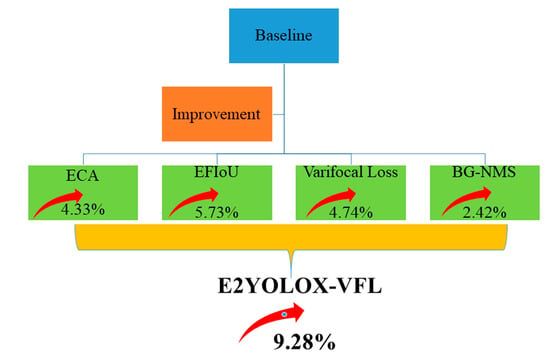
From the data in Table 2, it can be seen that replacing NMS with BG-NMS improves the mAP for ship detection by 2.42%. BG-NMS improves the accuracy of dense target detection, which can refer to Figure 5.
From Table 2, it becomes apparent that an enhancement is achieved by adding the ECA attention module to the Backbone network of the original model, which improves the mAP for ship detection by 4.33%. This enhancement improves the network’s feature extraction capability, allowing for better capture of target information and alleviating cases of missing small targets.
Replacing the confidence loss function with Varifocal Loss results in a 4.74% improvement in mAP for ship detection. This addresses the issues of imbalanced positive and negative samples and class imbalance.
By replacing the localization loss function with EFIoU Loss, the mAP for ship detection improves by 5.73%. This resolves the problem of regression failure when the two bounding boxes are not intersecting and the inability to reflect regression for targets of different sizes with the same aspect ratio.
When both the ECA attention module and EFIoU Loss are incorporated into the original model, the mAP for ship detection improves by 6.10%. This indicates that the joint improvement approach is effective. When all improvements are added to the original model, the mAP for ship detection improves by 9.28%. The outcomes obtained clearly illustrate the substantial influence of the proposed improvements.
Furthermore, the study compares the results of incorporating the ECA module into the Backbone network versus incorporating it into the FPN network. Additionally, upon reviewing Table 5, it is evident that the utilization of the ECA in this research, compared to the CBAM, achieves a slightly lower mAP by 0.44%, but with a reduction in parameters by 0.4MB. Incorporating the ECA module into the Backbone network demonstrates better results, with higher mAP and lower parameter quantity compared to incorporating it into the FPN network.
Additionally, the detection results in L3 of the E2YOLOX-VFL model were compared with the results in L3 of the SRBBS-Fast-RCNN and SRBBS-Fast-RCNN-R models reported in the literature proposing the HRSC20l6 [36] dataset and in Li et al. [64]. As observed from Table 6, the E2YOLOX-VFL model outperforms the results reported in [36], and it performs just a little lower than SHDRP9 in terms of ship detection mAP.
Figure 5 shows a comparison of the detection performance between the NMS approach and the BG-NMS approach. Figure 5a,c shows the detection results using the NMS approach, and Figure 5b,d shows the detection results using the BG-NMS approach. Despite some missed detections (in cases where prediction boxes of two targets overlap completely), the BG-NMS approach reduces instances of missing densely packed targets to some extent. Therefore, the BG-NMS algorithm exhibits better detection performance for densely packed targets.
To gain a more visual understanding of the detection performance of the E2YOLOX-VFL algorithm, the same image was subjected to detection using both the YOLOX and E2YOLOX-VFL networks. The detection results are depicted in Figure 6, where Figure 6a shows the detection result using YOLOX, and Figure 6b shows the detection result using E2YOLOX-VFL. It can be observed that the E2YOLOX-VFL algorithm performs better in detecting small targets and reduces instances of missing densely packed targets.
To illustrate how the new algorithm can improve the missed detection of densely packed targets, we compared the detection results of YOLOX and E2YOLOX-VFL in Figure 7. Figure 7a,c shows the detection result using YOLOX, and Figure 7b,d shows the detection result using E2YOLOX-VFL. It can be observed that the E2YOLOX-VFL algorithm can reduce instances of missing densely packed targets.
Figure 8 shows the effect of image enhancement. It can be seen that the target becomes clearer after image enhancement.
Applying the E2YOLOX-VFL algorithm to the location of a typhoon center, the results are shown in Figure 9. The mAP achieved using the E2YOLOX-VFL algorithm is 93.75%, outperforming YOLOX by 1.99%, which demonstrates the applicability of our method to other types of object detection and its overall effectiveness.
6. Conclusions
In this research, we propose an improved algorithm based on the YOLOX model, E2YOLOX-VFL, to address the challenges faced in ship detection in optical remote sensing imagery, such as background interference, variations in target size and position, and class imbalance. By incorporating the ECA module into the Backbone network, modifying the localization and confidence loss functions in YOLO Head, and improving the non-maximum suppression strategy, we enhance the model’s ability to detect occluded and multi-scale targets, address the issue of imbalanced positive and negative samples, and handle foreground–background imbalance. These improvements result in an enhanced robustness of the model. Experimental results demonstrate that the proposed E2YOLOX-VFL model achieves higher accuracy in ship detection compared to the original YOLOX model, and it performs favorably against other algorithms evaluated in this research. The model can be further applied to other types of object detection tasks.
Author Contributions
Conceptualization, Q.Z. and Y.W.; methodology, Q.Z.; software, Q.Z.; validation, Q.Z. and Y.Y.; formal analysis, Q.Z. and Y.Y.; investigation, Q.Z.; resources, Y.W.; data curation, Y.Y.; writing—original draft preparation, Q.Z.; writing—review and editing, Q.Z. and Y.W.; visualization, Q.Z.; supervision, Q.Z.; project administration, Y.W.; funding acquisition, Q.Z. All authors have read and agreed to the published version of the manuscript.
Funding
This research was funded by the National Natural Science Foundation of China, grant number 61573183, and Civil Aerospace during the 14th Five Year Plan period, guide number D010201.
Data Availability Statement
The data presented in this study are available on request from the corresponding author. The data are not publicly available due to copyright.
Acknowledgments
The authors are grateful for anonymous reviewers’ critical comments and constructive suggestions.
Conflicts of Interest
The authors declare no conflicts of interest.
References
- Bi, F.; Zhu, B.; Gao, L.; Bian, M. A Visual Search Inspired Computational Model for Ship Detection in Optical Satellite Images. IEEE Geosci. Remote Sens. Lett. 2012, 9, 749–753. [Google Scholar]
- Zhao, M.; Zhang, X.; Kaup, A. Multitask Learning for SAR Ship Detection with Gaussian-Mask Joint Segmentation. IEEE Trans. Geosci. Remote Sens. 2021, 14, 5214516. [Google Scholar] [CrossRef]
- Wan, H.; Huang, Z.; Xia, R.; Wu, B.; Sun, L.; Yao, B.; Liu, X.; Xing, M. AFSar: An Anchor-free SAR Target Detection Algorithm Based on Multiscale Enhancement Representation Learning. IEEE Trans. Geosci. Remote Sens. 2022, 60, 5219514. [Google Scholar] [CrossRef]
- Tang, J.; Deng, C.; Huang, G.; Zhao, B. Compressed-Domain Ship Detection on Spaceborne Optical Image Using Deep Neural Network and Extreme Learning Machine. IEEE Trans. Geosci. Remote Sens. 2015, 53, 1174–1185. [Google Scholar] [CrossRef]
- Zhu, C.; Zhou, H.; Wang, R.; Wang, R.; Guo, J. A Novel Hierarchical Method of Ship Detection from Spaceborne Optical Image Based on Shape and Texture Features. IEEE Trans. Geosci. Remote Sens. 2010, 48, 3446–3456. [Google Scholar] [CrossRef]
- He, S.; Yang, S.; Shi, A.; Li, T. Application of Texture Higher-Order Classification Feature in Ship Target Detection on The Sea. Opt. Electron. Technol. 2008, 6, 79–82. [Google Scholar]
- Zhang, D.; He, S.; Yang, S. A Multi-Scale Fractal Method for Ship Target Detection. Laser. Infrared. 2009, 39, 315–318. [Google Scholar]
- Li, C.; Hu, Y.; Chen, X. Research on Marine Ship Detection Method of SAR Image Based on Fuzzy Theory. Comput. App. 2005, 25, 1954–1956. [Google Scholar]
- Zhao, H.; Wang, P.; Dong, C.; Shang, Y. Ship Target Detection Using Multi-scale Visual Saliency. Optisc. Precis. Eng. 2020, 28, 1395–1403. [Google Scholar] [CrossRef]
- Wang, H.; Zhu, M.; Lin, C.; Chen, D.; Yang, H. Ship Detection in Complex Sea Background in Optical Remote Sensing Images. Optisc. Precis. Eng. 2018, 26, 723–732. [Google Scholar] [CrossRef]
- Zhang, C.; Xiong, B.; Kuang, G. Overview of Ship Target Detection in Optical Satellite Remote Sensing Images. J. Rad. Sci. 2020, 35, 637–647. [Google Scholar]
- Girshick, R.; Donahue, J.; Darrell, T.; Malik, J. Rich Feature Hierarchies for Accurate Object Detection and Semantic Segmentation. In Proceedings of the 2014 IEEE Conference on Computer Vision and Pattern Recognition, Columbus, OH, USA, 23–28 June 2014. [Google Scholar]
- Girshick, R. Fast R-CNN. In Proceedings of the 2015 IEEE International Conference on Computer Vision (ICCV), Santiago, Chile, 7–13 December 2015. [Google Scholar]
- Ren, S.; He, K.; Girshick, R.; Sun, J. Faster R-CNN: Towards Real-Time Object Detection with Region Proposal Networks. IEEE Trans. Pattern Anal. Mach. Intel. 2017, 39, 1137–1149. [Google Scholar] [CrossRef] [PubMed]
- Yang, L.; Su, J.; Huang, H.; Li, X. A Ship Target Detection Algorithm for SAR Images Based on Deep Multi-scale Feature Fusion CNN. J. Opt. 2020, 40, 0215002. [Google Scholar]
- Zhang, R.; Yao, J.; Zhang, K.; Chen, F.; Zhang, J. S-CNN-Based Ship Detection from High-Resolution Remote Sensing Images. In Proceedings of the International Archives of the Photogrammetry Remote Sensing and Spatial Information Sciences, Prague, Czech Republic, 12–19 July 2016. [Google Scholar]
- Ma, X.; Shao, L.; Jin, X. Ship Ttarget Detection Method in Visual Images Based on Improved Mask R-CNN. J. B. Univ. Technol. 2021, 41, 734–744. [Google Scholar]
- Han, X.; Zhong, Y.; Zhang, L. An Efficient and Robust Integrated Geospatial Object Detection Framework for High Spatial Resolution Remote Sensing Imagery. Remote Sens. 2017, 9, 666. [Google Scholar] [CrossRef]
- Li, Q.; Mou, L.; Liu, Q.; Wang, Y.; Zhu, X. HSF-Net: Multiscale Deep Feature Embedding for Ship Detection in Optical Remote Sensing Imagery. IEEE Trans. Geosci. Remote Sens. 2018, 56, 7147–7161. [Google Scholar] [CrossRef]
- Yao, Y.; Jiang, Z.; Zhang, H.; Zhao, D.; Cai, B. Ship Detection in Optical Remote Sensing Images Based on Convolutional Neural Networks. J. App. Remote Sens. 2017, 11, 042611. [Google Scholar] [CrossRef]
- Yang, F.; Xu, Q.; Li, B.; Ji, Y. Ship Detection from Thermal Remote Sensing Imagery through Region Based on Deep Forest. IEEE Geosci. Remote Sens. Lett. 2018, 15, 449–453. [Google Scholar] [CrossRef]
- Jiang, Y.; Zhu, X.; Zhang, W. Ship Extraction Using Post CNN from High Resolution Optical Remotely Sensed Images. In Proceedings of the 3rd Information Networking, Electronics and Automation Control Conference (ITNEC), Chengdu, China, 15–17 March 2019. [Google Scholar]
- Redmon, J.; Redmon, S.; Girshick, R.; Farhadi, A. You Only Look Once: Unified, Real-Time Object Detection. In Proceedings of the 2016 IEEE Conference on Computer Vision and Pattern Recognition (CVPR), Las Vegas, NV, USA, 27–30 June 2016. [Google Scholar]
- Redmon, J.; Farhadi, A. YOLO9000: Better, Faster, Stronger. In Proceedings of the 2017 IEEE Conference on Computer Vision and Pattern Recognition (CVPR), Honolulu, HI, USA, 21–26 July 2017. [Google Scholar]
- Chen, D.; Shao, H.; Zhang, J. Research on Improving YOLOv3′s Ship Detection Algorithm. Mod. Electron. Technol. 2023, 46, 101–106. [Google Scholar]
- Xu, Y.; Gu, Y.; Peng, D.; Liu, J.; Chen, H. An Improved YOLOv3 Model for Arbitrary Direction Ship Detection in Synthetic Aperture Radar Images. J. Mil. Eng. 2021, 42, 1698–1707. [Google Scholar]
- Zou, Z.; Shi, Z. Ship Detection in Spaceborne Optical Image with SVD Networks. IEEE Trans. Geosci. Remote Sens. 2016, 54, 5832–5845. [Google Scholar] [CrossRef]
- Wang, R.; Li, J.; Duan, Y.; Cao, H.; Zhao, Y. Study on the Combined Application of CFAR and Deep Learning in Ship Detection. J. Indian Soc. Remote Sens. 2018, 46, 1413–1421. [Google Scholar] [CrossRef]
- Zhu, X.; Lyu, S.; Wang, X. TPH-YOLOv5: Improved YOLOv5 Based on Transformer Prediction Head for Object Detection on Drone-Captured Scenarios. In Proceedings of the IEEE International Conference on Computer Vision Workshops(ICCVW), Montreal, BC, Canada, 11–17 October 2021. [Google Scholar]
- Wang, X.; Jiang, H.; Lin, K. Ship Detection in Remote Sensing Images Based on Improved YOLO Algorithm. J. B. Univ. Aeronaut. Astronaut. 2020, 46, 1184–1191. [Google Scholar]
- Zhang, D.; Wang, C.; Fu, Q. A Ship Critical Position Detection Algorithm Based on Improved YOLOv4 Tiny. Radio Eng. 2023, 53, 628–635. [Google Scholar]
- Li, J.; Zhang, D.; Fan, Y.; Yang, J. Lightweight Ship Target Detection Algorithm Based on Improved YOLOv5. Comput. App. 2023, 43, 923–929. [Google Scholar]
- Ge, Z.; Liu, S.; Wang, F.; Li, Z.; Ge, L. YOLOX: Exceeding YOLO Series in 2021. arXiv 2021, arXiv:2107.08430. [Google Scholar]
- Liu, F.; Chen, R.; Zhang, J.; Xing, K.; Liu, H.; Qin, J. R2YOLOX: A Lightweight Refined Anchor-Free Rotated Detector for Object Detection in Aerial Images. IEEE Trans. Geosci. Remote Sens. 2022, 60, 5632715. [Google Scholar] [CrossRef]
- Wang, Q.; Wu, B.; Zhu, P.; Li, P.; Zuo, W.; Hu, Q. ECA-Net: Efficient Channel Attention for Deep Convolutional Neural Networks. In Proceedings of the 2020 IEEE/CVF Conference on Computer Vision and Pattern Recognition (CVPR), Seattle, WA, USA, 13–19 June 2020. [Google Scholar]
- Liu, Z.; Yuan, L.; Weng, L.; Yang, Y. A High Resolution Optical Satellite Image Dataset for Ship Recognition and Some New Baselines. In Proceedings of the 6th International Conference on Pattern Recognition Applications and Methods (ICPRAM), Porto, Portugal, 24–26 February 2017. [Google Scholar]
- Howard, D.; Roberts, S.; Brankin, R. Target Detection in SAR Imagery by Genetic Programming. Adv. Eng. Softw. 1999, 5, 303–311. [Google Scholar] [CrossRef]
- Marre, F. Automatic vessel detection system on SPOT-5 optical imagery: A neuro-genetic approach. In Proceedings of the Fourth Meeting of the DECLIMS Project, Toulouse, France, 10–12 June 2004. [Google Scholar]
- Bentes, C.; Velotto, D.; Lehner, S. Target Classification in Oceanographic SAR Images with Dep Neural Networks: Architecture and Initial Results. In Proceedings of the 2015 IEEE International Geoscience and Remote Sensing Symposium, Milan, Italy, 26–31 July 2015. [Google Scholar]
- Bentes, C.; Frost, A.; Velotto, D.; Tings, B. Ship-Iceberg Discrimination with Convolutional Neural Networks in High Resolution SAR Images. In Proceedings of the 11th European Conference on Synthetic Aperture Radar Electronic Proceedings, Hamburg, Germany, 6–9 June 2016. [Google Scholar]
- Fernandez, V.; Velotto, D.; Tings, B.; Van, H.; Bentes, C. Ship Classification in High and Very High Resolution Satellite SAR Imagery. In Proceedings of the Future Security 2016, Stuttgart, Germany, 29–30 September 2016. [Google Scholar]
- Liu, G.; Zhang, Y.; Zheng, X.; Sun, X. A New Method on Inshore Ship Detection in High-Resolution Satellite Images Using Shape and Context Information. IEEE Geosci. Remote Sens. Lett. 2013, 11, 617–621. [Google Scholar] [CrossRef]
- Abadi, M.; Barham, P.; Chen, J.; Chen, Z.; Zhang, X. TensorFlow: A System for Large-Scale Machine Learning. arXiv 2016, arXiv:1605.08695. [Google Scholar]
- Yang, X.; Sun, H.; Fu, K.; Yang, J.; Sun, X.; Yan, M.; Guo, Z. Automatic Ship Detection of Remote Sensing Images from Google Earth in Complex Scenes Based on Multi-Scale Rotation Dense Feature Pyramid Networks. Remote Sens. 2018, 10, 132. [Google Scholar] [CrossRef]
- Liu, Z.; Hu, J.; Weng, L.; Yang, Y. Rotated region based CNN for ship detection. In Proceedings of the IEEE International Conference on Image Processing (ICIP), Beijing, China, 17–20 September 2017. [Google Scholar]
- Liu, W.; Ma, L.; Chen, H. Arbitrary-Oriented Ship Detection Framework in Optical Remote-Sensing Images. IEEE Geosci. Remote Sens. Lett. 2018, 15, 937–941. [Google Scholar] [CrossRef]
- Nie, M.; Zhang, J.; Zhang, X. Ship Segmentation and Orientation Estimation Using Keypoints Detection and Voting Mechanism in Remote Sensing Images. In Proceedings of the 16th International Symposium on Neural Networks (ISNN 2019), Moscow, Russia, 10–12 July 2019. [Google Scholar]
- Feng, Y.; Diao, W.; Sun, X.; Yan, M. Towards Automated Ship Detection and Category Recognition from High-Resolution Aerial Images. Remote Sens. 2019, 11, 1901. [Google Scholar] [CrossRef]
- Sun, J.; Zou, H.; Deng, Z.; Cao, X.; Li, M.; Ma, Q. Multiclass Oriented Ship Localization and Recognition in High Resolution Remote Sensing Images. In Proceedings of the 2019 IEEE International Geoscience and Remote Sensing Symposium, Yokohama, Japan, 28 July–2 August 2019. [Google Scholar]
- Cai, Z.; Vasconcelos, N. Cascade R-CNN: Delving into High Quality Object Detection. In Proceedings of the 2018 IEEE/CVF Conference on Computer Vision and Pattern Recognition, Salt Lake City, UT, USA, 18–23 June 2018. [Google Scholar]
- Wang, C.; Tian, J. Precise Recognition of Ship Target Based on Generative Adversarial Network Assisted Learning. J. Intell. Syst. 2020, 15, 296–301. [Google Scholar]
- Li, M.; Sun, W.; Zhang, X.; Yao, L. Fine Grained Recognition of Ship Targets in Optical Satellite Remote Sensing Images Based on Global Local Feature Combination. Spacecraft Rec. Remote Sens. 2021, 42, 138–147. [Google Scholar]
- Zhou, Q. Research on Ship Detection Technology in Ocean Optical Remote Sensing Images. Master’s Thesis, Institute of Optoelectronics Technology, Chinese Academy of Sciences, Chengdu, China, 2021. [Google Scholar]
- Yu, J.; Jiang, Y.; Wang, Z.; Huang, T. Unitbox: An Advanced Object Detection Network. In Proceedings of the 24th ACM International Conference on Multimedia, Amsterdam, The Netherlands, 1 October 2016. [Google Scholar]
- Rezatofighi, H.; Tsoi, N.; Gwak, J.; Sadeghian, A.; Savarese, S. Generalized Intersection over Union: A Metric and A Loss for Bounding Box Regression. In Proceedings of the 2019 IEEE/CVF Conference on Computer Vision and Pattern Recognition (CVPR), Long Beach, CA, USA, 15–20 June 2019. [Google Scholar]
- Zheng, Z.; Wang, P.; Liu, W.; Li, J.; Ye, R.; Ren, D. Distance-IoU Loss: Faster and Better Learning for Bounding Box Regression. arXiv 2019, arXiv:1911.08287. [Google Scholar] [CrossRef]
- Zhang, Y.; Ren, W.; Zhang, Z.; Jia, Z.; Wang, L.; Tan, T. Focal and Efficient IoU loss for Accurate Bounding Box Regression. arXiv 2022, arXiv:2101.08158. [Google Scholar] [CrossRef]
- Liu, S.; Huang, D.; Wang, Y. Adaptive NMS: Refining Pedestrian Detection in A Crowd. In Proceedings of the 2019 IEEE/CVF Conference on Computer Vision and Pattern Recognition (CVPR), Long Beach, CA, USA, 15–20 June 2019. [Google Scholar]
- Navaneeth, B.; Bharat, S.; Rama, C.; Davis, L. Soft-NMS-Improving Object Detection with One Line of Code. In Proceedings of the 2017 IEEE International Conference on Computer Vision (ICCV), Venice, Italy, 24–27 October 2017. [Google Scholar]
- Li, X.; Yu, L.; Chang, D.; Ma, Z.; Cao, J. Dual Cross-Entropy Loss for Small-Sample Fine-Grained Vehicle Classification. IEEE Trans. Vehi. Tech. 2019, 68, 4204–4212. [Google Scholar] [CrossRef]
- Zhang, H.; Wang, Y.; Dayoub, F.; Sünderhauf, N. VarifocalNet: An IoU-Aware Dense Object Detector. In Proceedings of the 2021 IEEE/CVF Conference on Computer Vision and Pattern Recognition (CVPR), Nashville, TN, USA, 20–25 June 2021. [Google Scholar]
- An, H.; Rodrigo, B.; Bernt, S. Learning Non-Maximum Suppression. In Proceedings of the 2017 IEEE Conference on Computer Vision and Pattern Recognition (CVPR), Honolulu, HI, USA, 21–26 July 2017. [Google Scholar]
- Jiang, S. Research on Ship Detection Method of Optical Remote Sensing Image Based on Deep Learning. Master’s Thesis, School of Electronic Information Engineering, Shanghai Jiao Tong University, Shanghai, China, 2019. [Google Scholar]
- Li, B.; Xie, X.; Wei, X.; Tang, W. Ship detection and classification from optical remote sensing images: A survey. Chin. J. Aeronaut. 2021, 343, 145–163. [Google Scholar] [CrossRef]
Figure 1.
Overall network architecture of E2YOLOX-VFL.

Figure 2.
Simplified diagram of calculation process. Different colors represent the upper and lower rows of elements.
Figure 2.
Simplified diagram of calculation process. Different colors represent the upper and lower rows of elements.

Figure 3.
L3 class number distribution.

Figure 4.
Epoch_loss change curve.

Figure 5.
Comparison of detection performance between NMS and BG-NMS approach: (a,c) NMS detection result, (b,d) BG-NMS detection result.
Figure 5.
Comparison of detection performance between NMS and BG-NMS approach: (a,c) NMS detection result, (b,d) BG-NMS detection result.

Figure 6.
Comparison of detection performance between the original and improved algorithms: (a)YOLOX detection result, (b) E2YOLOX-VFL detection result.
Figure 6.
Comparison of detection performance between the original and improved algorithms: (a)YOLOX detection result, (b) E2YOLOX-VFL detection result.

Figure 7.
Comparison of detection performance of dense targets between the original and improved algorithms: (a,c) YOLOX detection result, (b,d) E2YOLOX-VFL detection result.
Figure 7.
Comparison of detection performance of dense targets between the original and improved algorithms: (a,c) YOLOX detection result, (b,d) E2YOLOX-VFL detection result.


Figure 8.
The effect of image enhancement: (a) without image enhancement, (b) with image enhancement.
Figure 8.
The effect of image enhancement: (a) without image enhancement, (b) with image enhancement.

Figure 9.
The performance of the algorithm in locating the center of a typhoon: (a) original typhoon image, (b) positioning typhoon center image, (c) YOLOX’s mAP, (d) E2YOLOX-VFL’s mAP.
Figure 9.
The performance of the algorithm in locating the center of a typhoon: (a) original typhoon image, (b) positioning typhoon center image, (c) YOLOX’s mAP, (d) E2YOLOX-VFL’s mAP.


Table 1.
Networks used for training.
| Networks | Illustrate |
|---|---|
| YOLOX | Original network |
| YOLOX-BGNMS | Change NMS to BGNMS |
| YOLOX-ECA | Add ECA module to YOLOX Backbone |
| YOLOX-VFL | Change the confidence loss of YOLOX from CE to Varifocal Loss |
| YOLOX-EFIoU | Change the confidence loss of YOLOX from IoU Loss to EFIoU Loss |
| E2YOLOX | Add ECA module to YOLOX Backbone, and change the location loss from IoU Loss to EFIoU Loss |
| E2YOLOX-VFL | Add ECA module to YOLOX Backbone, change NMS to BG-NMS, change the confidence loss from CE to Varifocal Loss, and change the location loss from IoU Loss to EFIoU Loss |
Table 2.
Results of ablation experiments.
| Module | YOLOX | BG-NMS | ECA | Varifocal Loss | EFIoU | mAP/% | |
|---|---|---|---|---|---|---|---|
| Model | |||||||
| YOLOX 1 | √ | × | × | × | × | 64.54 | |
| YOLOX 2 | √ | × | × | × | × | 64.82 | |
| YOLOX-BGNMS | √ | √ | × | × | × | 66.96 | |
| YOLOX-ECA | √ | × | √ | × | × | 68.87 | |
| YOLOX-VFL | √ | × | × | √ | × | 69.28 | |
| YOLOX-EFIoU | √ | × | × | × | √ | 70.27 | |
| E2YOLOX | √ | × | √ | × | √ | 70.64 | |
| E2YOLOX-VFL | √ | √ | √ | √ | √ | 73.82 | |
Footnote: YOLOX 2 is the result of image enhancement, and YOLOX 1 represents the result without image enhancement.
Table 3.
The results of adding ECA after the three feature layers.
| Module | ECA | ECA | ECA | mAP/% | |
|---|---|---|---|---|---|
| Model | |||||
| YOLOX | × | × | × | 64.54 | |
| (80, 80) | √ | × | × | 66.36 | |
| (40, 40) | √ | √ | × | 67.13 | |
| (20, 20) | √ | √ | √ | 68.87 | |
Table 4.
The results of EIoU and EFIoU.
| Module | EIoU | EFIoU | mAP/% | |
|---|---|---|---|---|
| Model | ||||
| YOLOX | × | × | 64.54 | |
| YOLOX-EIoU | × | √ | 67.57 | |
| YOLOX-EFIoU | × | √ | 70.27 | |
Table 5.
Improvement results when adding different modules and adding ECA in different positions.
| Model | mAP/% | Parameter Quantity |
|---|---|---|
| Adding CBAM to the Backbone | 69.31 | 34.7 MB |
| Adding ECA to the Backbone | 68.87 | 34.3 MB |
| Adding ECA to the FPN | 61.75 | 55.2 MB |
Table 6.
Detection results of different models in the HRSC2016 dataset (L3).
| Model | mAP/% |
|---|---|
| E2YOLOX-VFL | 73.82 |
| SRBBS-Fast-RCNN | 60.77 |
| SRBBS-Fast-RCNN-R | 45.23 |
| RC1 | 51.0 |
| RC1 + Multi-NMS | 43.7 |
| Faster R-CNN | 40.5 |
| R-DFPN | 43.5 |
| R-DFPN + PSG97 | 71.0 |
| SHDRP9 | 74.2 |
Disclaimer/Publisher’s Note: The statements, opinions and data contained in all publications are solely those of the individual author(s) and contributor(s) and not of MDPI and/or the editor(s). MDPI and/or the editor(s) disclaim responsibility for any injury to people or property resulting from any ideas, methods, instructions or products referred to in the content. |
© 2024 by the authors. Licensee MDPI, Basel, Switzerland. This article is an open access article distributed under the terms and conditions of the Creative Commons Attribution (CC BY) license (https://creativecommons.org/licenses/by/4.0/).
Share and Cite
MDPI and ACS Style
Zhao, Q.; Wu, Y.; Yuan, Y. Ship Target Detection in Optical Remote Sensing Images Based on E2YOLOX-VFL. Remote Sens. 2024, 16, 340. https://0-doi-org.brum.beds.ac.uk/10.3390/rs16020340
AMA Style
Zhao Q, Wu Y, Yuan Y. Ship Target Detection in Optical Remote Sensing Images Based on E2YOLOX-VFL. Remote Sensing. 2024; 16(2):340. https://0-doi-org.brum.beds.ac.uk/10.3390/rs16020340
Chicago/Turabian StyleZhao, Qichang, Yiquan Wu, and Yubin Yuan. 2024. "Ship Target Detection in Optical Remote Sensing Images Based on E2YOLOX-VFL" Remote Sensing 16, no. 2: 340. https://0-doi-org.brum.beds.ac.uk/10.3390/rs16020340
Note that from the first issue of 2016, this journal uses article numbers instead of page numbers. See further details here.