Article

Retrieval of Melt Ponds on Arctic Multiyear Sea Ice in Summer from TerraSAR-X Dual-Polarization Data Using Machine Learning Approaches: A Case Study in the Chukchi Sea with Mid-Incidence Angle Data

1
Division of Polar Ocean Environment, Korea Polar Research Institute (KOPRI), Incheon 29190, Korea
2
School of Urban and Environmental Engineering, Ulsan National Institute of Science and Technology (UNIST), Ulsan 44919, Korea
3
Space Imaging Research & Development Lab., LIG Nex1 Co., Ltd., Yongin 16911, Korea
4
School of Earth and Environmental Sciences, Seoul National University, Seoul 08826, Korea
*
Author to whom correspondence should be addressed.
Submission received: 10 September 2015 / Revised: 31 December 2015 / Accepted: 6 January 2016 / Published: 12 January 2016
(This article belongs to the Special Issue Sea Ice Remote Sensing and Analysis)

Abstract

:
Melt ponds, a common feature on Arctic sea ice, absorb most of the incoming solar radiation and have a large effect on the melting rate of sea ice, which significantly influences climate change. Therefore, it is very important to monitor melt ponds in order to better understand the sea ice-climate interaction. In this study, melt pond retrieval models were developed using the TerraSAR-X dual-polarization synthetic aperture radar (SAR) data with mid-incidence angle obtained in a summer multiyear sea ice area in the Chukchi Sea, the Western Arctic, based on two rule-based machine learning approaches—decision trees (DT) and random forest (RF)—in order to derive melt pond statistics at high spatial resolution and to identify key polarimetric parameters for melt pond detection. Melt ponds, sea ice and open water were delineated from the airborne SAR images (0.3-m resolution), which were used as a reference dataset. A total of eight polarimetric parameters (HH and VV backscattering coefficients, co-polarization ratio, co-polarization phase difference, co-polarization correlation coefficient, alpha angle, entropy and anisotropy) were derived from the TerraSAR-X dual-polarization data and then used as input variables for the machine learning models. The DT and RF models could not effectively discriminate melt ponds from open water when using only the polarimetric parameters. This is because melt ponds showed similar polarimetric signatures to open water. The average and standard deviation of the polarimetric parameters based on a 15 × 15 pixel window were supplemented to the input variables in order to consider the difference between the spatial texture of melt ponds and open water. Both the DT and RF models using the polarimetric parameters and their texture features produced improved performance for the retrieval of melt ponds, and RF was superior to DT. The HH backscattering coefficient was identified as the variable contributing the most, and its spatial standard deviation was the next most contributing one to the classification of open water, sea ice and melt ponds in the RF model. The average of the co-polarization phase difference and the alpha angle in a mid-incidence angle were also identified as the important variables in the RF model. The melt pond fraction and sea ice concentration retrieved from the RF-derived melt pond map showed root mean square deviations of 2.4% and 4.9%, respectively, compared to those from the reference melt pond maps. This indicates that there is potential to accurately monitor melt ponds on multiyear sea ice in the summer season at a local scale using high-resolution dual-polarization SAR data.

Graphical Abstract

1. Introduction

The sea ice cover in the Arctic has declined since the beginning of satellite observation in 1979 [1,2,3,4,5,6], which has a strong influence on the changes of climate systems, marine ecosystems and maritime resource development [7,8,9]. The seasonal decline of the Arctic sea ice extent has been dramatic from summer (−70.1 ± 7.8 × 10³ km2·y−1) to autumn (−57.3 ± 5.7 × 10³ km2·y−1) for the past 30 years [1]. The Arctic sea ice decline in summer and autumn can be amplified by the development of melt ponds that can cover up to 50%–60% of the sea ice area [10,11]. While snow-covered and bare sea ice have a high surface albedo, melt ponds reflect ~20% of the incident solar radiation and absorb four-times more solar energy than sea ice [12,13]. Ponded ice experiences more melting than snow-covered and bare sea ice due to the absorption of more solar energy [14], which plays a key role in the decline of sea ice in the Arctic [14,15,16]. Therefore, an accurate observation of melt ponds on the Arctic sea ice is critical in order to better understand the dynamics of sea ice decline and to provide important parameters for climate change research.
Optical satellite data with medium-low resolution (30 m–1 km), such as the Terra/Aqua Moderate Resolution Imaging Spectroradiometer (MODIS), the ENVISAT Medium Resolution Imaging Spectrometer (MERIS) and the Landsat-7 Enhanced Thematic Mapper Plus (ETM+), multispectral images have been used to observe melt ponds on widely-distributed sea ice in the Arctic [17,18,19,20,21,22,23]. Based on the distinctive spectral albedo of melt pond between sea ice and open water [22], the previous studies estimated the fraction of ponds by analyzing the albedo of ponded ice. The melt pond fraction estimated from the optical data resulted in a root mean square error (RMSE) of ~15% when compared to in situ observation and aerial photography [17,19,20,21,23], and it was used as an important predictor of sea ice cover and climate change [16,24,25]. However, the applicability of such optical images is restricted to daytime and clear skies, which provides few chances to observe the sea ice surface in the Arctic.
Synthetic aperture radar (SAR) has been widely used to observe sea ice and melt ponds because it provides surface images regardless of weather conditions and sun altitudes. Yackel and Barber [26] investigated the utility of radar backscattering to detect melt ponds using RADARSAT-1 SAR images in HH polarization. They found that the RADARSAT-1 HH backscattering coefficient and melt pond fraction of first-year sea ice in the Canadian Archipelago showed a strong positive relationship under windy conditions, but a very weak positive relationship under low wind speed. Mäkynen et al. [27] compared the backscattering coefficient of ENVISAT wide swath mode (WSM) SAR images in HH polarization to the melt pond fraction of the Arctic sea ice derived from MODIS images. Their results showed that the correlation between the backscattering coefficient and melt pond fraction was very low due to the low resolution of the WSM images (100 m). Kim et al. [28] retrieved the melt pond fraction of sea ice in the northern Chukchi Sea from a TerraSAR-X HH-polarized SAR amplitude image obtained in Stripmap mode. Although the TerraSAR-X Stripmap image has a fine spatial resolution (3 m), the melt pond fraction was largely underestimated. The previous studies with single-polarization SAR data have limitations in the retrieval of melt ponds. This is because the single-polarized backscattering coefficient depends mainly on surface roughness, and thus, it has limited information for identifying the ponds.
Polarimetric SAR measures radar backscattering from multi-polarization channels, which can provide a number of parameters representing various physical properties of a target that have been widely used for land cover classification [29,30,31]. Several studies demonstrated that a co-polarization ratio (the ratio of backscattering derived from VV and HH polarization), one of the polarimetric parameters, can identify melt ponds on first-year sea ice due to an obvious contrast of the dielectric property between the ponds and ice [32,33]. Scharien et al. [34] estimated the melt pond fraction on first-year ice in the Canadian Archipelago using the co- and cross-polarization ratios of RADARSAT-2 dual-polarimetric SAR data based on surface scattering theory. However, their approach showed weak performance for the sea ice with wet snow, which produced values similar to the polarization ratio for melt ponds.
As stated above, most of the previous studies using SAR had limitations for retrieving melt ponds because the backscattering coefficient and the polarization ratio were not enough to discriminate melt ponds from sea ice and open water. The use of a combination of polarimetric parameters computed from multi-polarization SAR can provide more physical properties of the ice surface than single polarimetric parameters [35,36]. Therefore, high-resolution polarimetric parameters can improve the performance of melt pond retrieval from SAR data, which can produce accurate statistics for melt ponds and sea ice. Most of the previous studies using polarimetric SAR focused on melt ponds on first-year ice [32,33,34], while few studies were performed for multiyear ice. Melt ponds on multiyear ice show different physical and microwave scattering characteristics from those on first-year ice [37]. Since polarimetric features from melt ponds on multiyear ice are likely different from those on first-year ice, melt pond retrievals from polarimetric SAR data should be further examined and evaluated for multiyear ice.
The objectives of this paper are to: (1) develop a novel approach to the retrieval of melt ponds on summer multiyear ice in the Chukchi Sea, the Western Arctic, for deriving accurate pond statistics using various polarimetric parameters derived from TerraSAR-X dual-polarization data based on the rule-based machine learning algorithms; (2) evaluate the performance of machine learning models for retrieving melt ponds; (3) identify key contributing variables for melt pond retrievals; and (4) investigate the robustness of the pond statistics obtained from high-resolution multi-polarization SAR data. The TerraSAR-X dual-polarization data and airborne SAR images used in this study and a brief explanation of the sea ice conditions in the study area are presented in Section 2. The methodology for developing melt pond detection models using the TerraSAR-X dual-polarization data based on machine learning approaches is described in Section 3. Results from the melt pond detection models and a discussion are covered in Section 4. Section 5 concludes this paper.

2. Materials

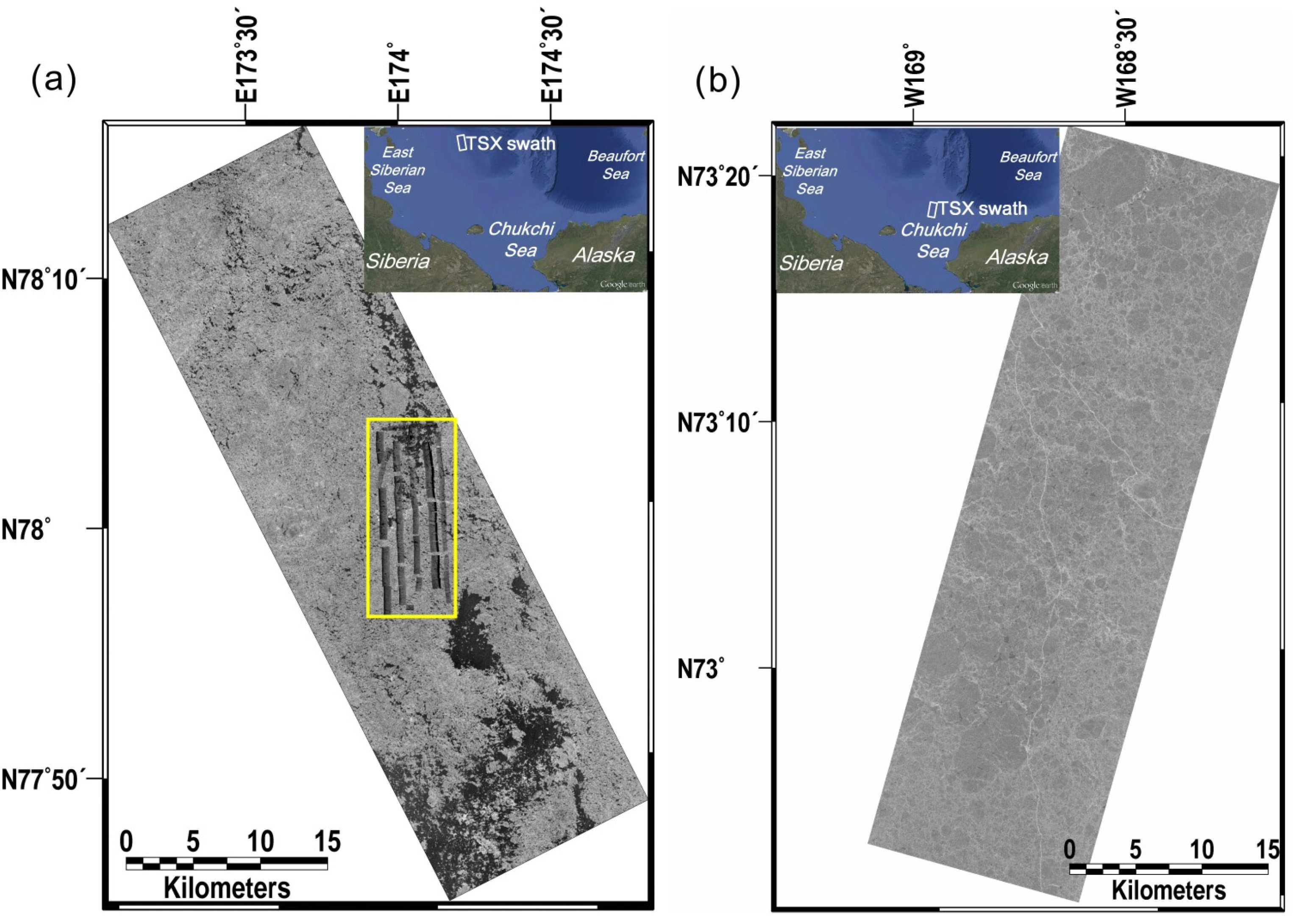
2.1. Airborne SAR Survey Data

Airborne X-band SAR (with a center frequency of 10.25 GHz) images with 0.3-m resolution acquired on 12 August 2011 in the northern Chukchi Sea (Figure 1) were used to construct a reference dataset for developing the melt pond detection models. The airborne SAR system was equipped with a Global Positioning System/inertial measurement units (GPS/IMUs) and a gimbal-mounted phased array antenna, which was mounted on a helicopter (Bell 206 Jet Ranger) and surveyed from 04:48 coordinated universal time (UTC) for 1 h. Due to technical problems, the airborne SAR images could not be combined into a perfectly continuous strip image [28]. Each original airborne SAR image has a size of approximately 600 m in the range direction by 350 m in the azimuth direction. However, the near-range part of the SAR images was cropped, leaving a size of approximately 400 m in the range direction by 350 m in the azimuth direction, due to no backscattered signal in a predetermined time domain [28]. In order to reduce speckle noise, the resolution of the original SAR images was downgraded to 0.6 m.
Figure 1. TerraSAR-X (TSX) amplitude images (HH-polarization) obtained in the Chukchi Sea on (a) 12 August 2011 and (b) 21 July 2010, respectively. The airborne SAR images are overlaid on the 2011 TerraSAR-X amplitude image (yellow box). The TerraSAR-X imaging area corresponds to the white solid box in each map.
Remotesensing 08 00057 g001

2.2. TerraSAR-X Dual-Polarization Data

TerraSAR-X is equipped with X-band SAR, a center frequency of 9.65 GHz, which provides high-resolution images in different imaging modes: 1 m in High-resolution Spotlight (HS), 2 m in Spotlight (SL), 3 m in most of Stripmap (SM) and 18 m in ScanSAR (SC) mode [38,39]. Dual-polarization data can be acquired in the TerraSAR-X imaging modes except for SC. In this study, two TerraSAR-X SM dual-polarization (HH and VV polarization) data with a mid-incidence angle of 32.7° acquired in a descending orbit at 18:15 UTC on 21 July 2010 and in an ascending orbit at 04:55 UTC on 12 August 2011 (the same date as the airborne SAR survey) were used for melt pond detection from summer multiyear sea ice in the northern Chukchi Sea (Figure 1). The swath width of the TerraSAR-X data was about 17 km. The TerraSAR-X data obtained in 2011 (Figure 1a) were used to develop and validate melt pond retrieval models based on machine learning approaches using the airborne SAR images. The other 2010 TerraSAR-X data were used to evaluate the machine learning model developed from the TerraSAR-X data in 2011. The TerraSAR-X data were delivered in a single-look complex (SLC) format. A 5 by 5 Lee filter [40] was applied to the TerraSAR-X SLC data in order to reduce speckle noise. The backscattering coefficients and different polarimetric parameters were derived from the filtered SLC data. The noise equivalent sigma zero (NESZ) of our TerraSAR-X data is −25 dB. A detailed description of the computation of the polarimetric parameters will be presented in Section 3.

2.3. Sea Ice Conditions
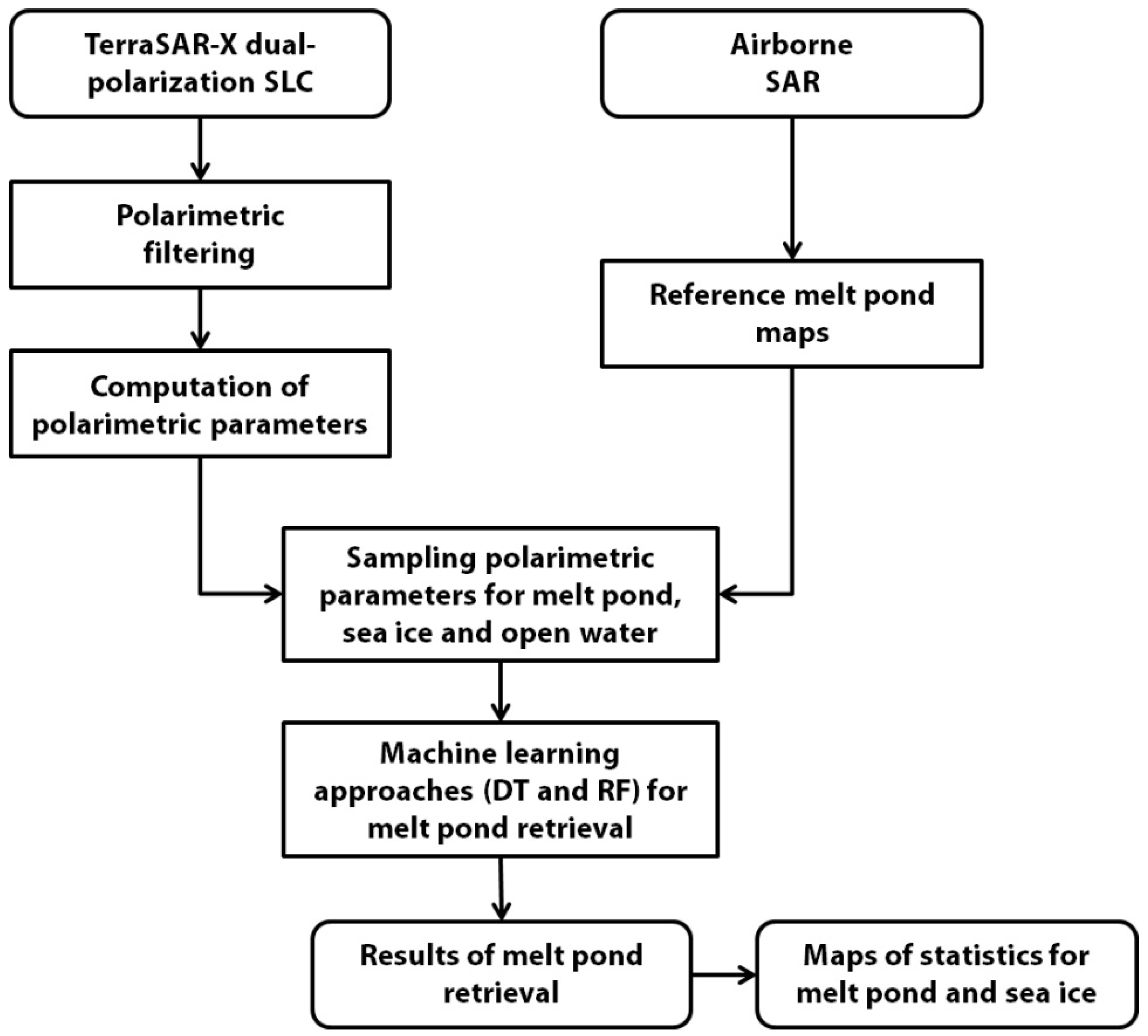
While a field survey of sea ice conditions in the area of TerraSAR-X data in 2010 was not performed, sea ice in the area was visually examined through analyzing the amplitude image (Figure 1a). In the 2010 TerraSAR-X image, large multiyear ice floes that hold numerous melt ponds, seen as dark in small sized and some large and dark open water, were observed. Kim et al. [28] provided sea ice conditions in the area of the TerraSAR-X data obtained in 2011 through the analysis of the aerial photographs acquired coincident with the airborne SAR survey (see Figures 4 and 9 in [28]). The study area consists of two sea ice conditions: one is large and thick multiyear ice floes that hold many melt ponds (more than 1000 per square kilometer) on the surface, while the other is heavily-melted small ice fragments of about 100 m in size that hold few melt ponds on the surface [28]. The aerial photographs showed that most of the melt ponds were interconnected by small channels. Such small channels could not be detected in the airborne SAR images, but would not significantly affect the estimation of the melt pond fraction, pond area and the number density of melt ponds from the SAR images [28]. Melt ponds observed in the airborne SAR images appeared in a very dark tone, which indicates that the wind speed was low, and thus, the surface of the ponds and open water would be smooth. Few shadow areas on the sea ice surface were observed from the airborne SAR images, which implies that the spatial variation of the ice topography was low.

3. Methodology

In this study, machine learning-based classification approaches were used to retrieve melt ponds on multiyear ice, in which the backscattering and polarimetric parameters of the TerraSAR-X dual-polarization data were used as input variables. Figure 2 shows the processing flow of the classification approach. This section presents the construction method of the reference dataset from the airborne SAR images, the computation of different polarimetric parameters and two rule-based machine learning approaches used for the classification of open water, sea ice and melt pond. The computation of various statistics for melt ponds is also described in this section.
Figure 2. Processing flow of the melt pond retrieval from the classification of the TerraSAR-X dual-polarization SAR data based on machine learning approaches. SLC, single-look complex; DT, decision tree; RF, random forest.
Remotesensing 08 00057 g002

3.1. Construction of the Reference Dataset

In order to construct a reference dataset for the classification of open water, sea ice and melt pond, the objects of each class were delineated from the airborne SAR images using a combination of multiscale segmentation and aggregation methods, as described in Kim et al. [28]. First, water and ice were classified from the object extraction procedure. The water objects within the ice were defined as melt ponds, while other water objects were defined as open water. In some airborne SAR images, open water within interconnected ice floes was misclassified as a melt pond. To reduce the misclassification of open water, the melt pond objects with an area larger than 700 m2 were considered to be open water [28]. This filtering process can change some large melt ponds to open water. However, such large melt ponds account for only 4% of the total number of melt ponds [28].
Kim et al. [28] evaluated the results of melt pond extraction from the airborne SAR images by one-to-one visual comparison with the aerial photographs (see Figure 9 in [28]). The shape and the size of melt ponds extracted from the airborne SAR images agreed with those from the aerial photographs. Some melt ponds were interconnected by small channels, which were identified in the aerial photographs. The small channels were not detected in the airborne SAR images, which would affect the estimation of pond circularity. However, the estimation of pond areas would not be significantly affected [28]. This suggests that the classification results of the airborne SAR images were accurate enough to be used as a reference dataset for the classification of the TerraSAR-X data.
The statistics for melt ponds, i.e., melt pond fraction ( F p ), number density of ponds ( N d ), mean pond size ( S p ) and sea ice concentration, were computed from the individual airborne SAR images. F p is defined as the percentage of total ice area covered by melt ponds, which is computed by [14]:
F p = A p / ( A i + A p )
where A p is the fraction of melt ponds within an airborne SAR image and A i is the fraction of sea ice excluding melt pond areas within the image. N d is defined as the number of melt ponds divided by the area of sea ice including melt ponds ( A i + A p ), with units of km−2 [14]. Sea ice concentration is defined as the fraction of sea ice including melt pond areas within the image.

3.2. Polarimetric Parameters

Polarimetric parameters derived from multi-polarization SAR data provide informative descriptions of the scattering mechanism of a target, and thus, can be very useful for the classification of different surface types. In this study, the dual-polarimetric 2 × 2 coherency matrix ( T 2 ) for the TerraSAR-X data was applied as follows [41]:
T 2 = 1 2 [ ( S H H + S V V ) ( S H H + S V V ) * ( S H H + S V V ) ( S H H S V V ) * ( S H H S V V ) ( S H H + S V V ) * ( S H H S V V ) ( S H H S V V ) * ]
where S X X is the scattering matrix complex element and superscript indicates the complex conjugation. Subscript X X indicates polarization. represents the ensemble average of the complex product. The drawback of the T 2 matrix is that it cannot provide information about the cross-polarization correlation coefficient and phase difference as obtainable from fully-polarimetric SAR data. Nevertheless, the dual-polarization SAR data can produce various polarimetric parameters. A total of 8 polarimetric parameters, including HH and VV backscattering coefficients, co-polarization ratio, co-polarization phase difference, co-polarization correlation coefficient, alpha angle, entropy and anisotropy, were derived from the TerraSAR-X dual-polarization data. The backscattering coefficients at HH ( σ H H 0 ) and VV polarization ( σ V V 0 ) in dB were derived from the filtered TerraSAR-X SLC data. The co-polarization ratio ( σ V V 0 / σ H H 0 in dB) was calculated from the backscattering coefficients. The phase difference ( ϕ H H V V ) and the correlation coefficient ( ρ H H V V ) were calculated as:
ϕ H H V V = arg ( S H H S V V * )
ρ H H V V = | S H H S V V * | σ V V 0 σ H H 0
where | | stands for the modulus of the complex product.
The entropy ( H )/anisotropy ( A )/alpha angle ( α ¯ ) decomposition [42] is based on the well-known polarimetric decomposition theorem that is useful in characterizing the scattering properties of various scattering media and, thus, widely used for land cover and land use classification [36,43]. H indicates the randomness of scattering mechanisms. A describes the relative power of secondary and tertiary scattering mechanisms for quad polarization data, but it is not defined for dual polarization data. For dual polarization data, A can be interpreted in terms of the number of scattering mechanisms by explaining with H [44]. α ¯ is an indicator of the type of scattering mechanism. The H / A / α ¯ decomposition was originally proposed for full-polarization data, but Cloude [45] modified the theory for dual-polarization data. H and A were calculated using the eigenvalues λ 1 and λ 2 of the T 2 matrix evaluated from the linear combinations of the scattering matrix elements as follows [45]:
H = P 1 log 2 ( P 1 ) P 2 log 2 ( P 2 )
A = P 1 P 2 P 1 + P 2
where P i ( i = 1 , 2 ) is the probability of each eigenvalue contribution, defined as:
P 1 = λ 1 λ 1 + λ 2 , P 2 = λ 2 λ 1 + λ 2
α ¯ was calculated using the dominant scattering alpha angle ( α ) as follows [45]:
α ¯ = P 1 α + P 2 ( π 2 α ) , α = cos 1 | x 1 | | ν 1 |
where x 1 is the first coordinate of the first eigenvector and | ν 1 | is the norm of the first eigenvector. The detailed evaluation of the coherency matrix, including the eigenvalue-eigenvector analysis, is described in Cloude and Pottier [42], Cloude [45] and Lee and Pottier [41]. All polarimetric parameters were projected into a Universal Transverse Mercator (UTM) projection (Zone 59 North) with a pixel size of 3 m.

3.3. Machine Learning Approaches for Melt Pond Retrieval

The surface type of the study area (open water, sea ice and melt pond) was set to a dependent variable for classification. To train and validate the machine learning-based classification models, a total of 37,152 samples (i.e., pixels) of polarimetric parameters for open water, sea ice and melt pond (12,384 samples for each class) were selected from the TerraSAR-X dual-polarization data by referring to the location of the objects of each class delineated from the airborne SAR images. As melt ponds on sea ice formed in a much smaller size than open water, the average and standard deviation of the polarimetric parameters might contribute to improve the machine learning-based classification models. In this study, the average and standard deviation (texture features) of the polarimetric parameters computed within a moving window with a size ranging from 5 × 5 to 35 × 35 pixels were calculated and used as additional input variables for the machine learning models. As the polarimetric parameters were projected with a pixel spacing of 3 m, objects with a size larger than 3 × 3 m were referred from the airborne SAR images. Eighty percent of the samples for each class (9907 samples) were randomly selected to be used as a training dataset, while the remaining samples (2477 samples for each class) were used as a test dataset in order to validate the models.
Machine learning is a novel approach used in various remote sensing applications, including land cover/land use classification [46,47,48,49,50,51,52], change detection [53,54], geological mapping [55], vegetation mapping [56,57,58,59], hydrological studies [60,61,62] and atmospheric studies [63,64]. In this study, two rule-based machine learning approaches—decision tree (DT) and random forest (RF)—were used for the classification of open water, sea ice and melt pond from the TerraSAR-X dual-polarization data. See5, developed by RuleQuest Research, Inc. (Empire Bay, Australia) [65], was used to carry out the DT-based classification. See5 uses repeated binary splits based on an entropy-related metric to develop a tree. The generated tree can be simplified and converted into a series of if-then rules, which makes it easy to analyze the classification results. RF creates multiple bootstrapped samples of the original training data and builds a set of no pruning classification and regression trees (CART) [66] from each set of bootstrapped samples, which is a rule-based decision tree. The numerous independent trees are grown by randomly selecting a subset of the training samples for each tree and a subset of splitting variables at each node of the tree, which overcomes the well-known limitation of CART that classification results largely depend on the configuration and quality of training samples [67]. For classification, each tree gives a unit vote for the most popular class at each input instance. A final conclusion from the independent decision trees is determined by using either a simple majority voting or weighted majority voting strategy. In this study, RF was implemented using an add-on package in the R software. See5 and RF produce information on the relative importance of input variables with attribute usage and mean decrease accuracy, respectively. The attribute usage information indicates how often each variable is used in the rules, while mean decrease accuracy represents the decrease in the accuracy of the model using out-of-bag data when a variable is randomly permuted. In other words, the attribute usage in See5 is reported by the percentage of the training cases where an attribute (i.e., the input variables) is used in predicting a class. The mean decrease accuracy in random forest is obtained by subtracting the number of correctly-classified cases for the variable-permuted out-of-bag data from the number of cases for original out-of-bag data and averaging the numbers for every tree in the forest. Therefore, the mean decrease accuracy means the average increase in the misclassification rate as a percentage. DT and RF are quickly trained, and it is easy to understand the model that was built for classification. Moreover, in general, RF outperforms artificial neural networks and the maximum likelihood classifier, especially when faced with a limited number of training samples and a large number of input variables [68].
To evaluate the performance of the machine learning models, typical accuracy metrics, including user’s accuracy, producer’s accuracy, overall accuracy and the kappa coefficient of agreement, were computed from a confusion matrix of the test dataset. User’s and producer’s accuracies show how well individual classes were classified correctly. The producer’s accuracy refers to the probability that a certain surface type of an area is correctly classified as such, while the user’s accuracy refers to the probability that a sample labeled as a surface type class is correctly classified as this class. Overall accuracy can be derived from dividing the number of samples that were correctly classified by the total number of samples. The kappa coefficient, another criterion used for the assessment of classification results, measures the degree of agreement between classification and reference data considering change agreement occurring by chance. The overall accuracy and the kappa coefficient have been widely used for accuracy assessment of the classification of remote sensing data [69,70,71]. The statistics for melt ponds were calculated from the results of the machine learning models and compared to those from the airborne SAR images, evaluating the feasibility of obtaining reliable pond statistics from the high-resolution dual-polarization SAR data. Quantitative accuracy assessment was performed on the classification of 2011 SAR data, and only visual assessment based on the SAR amplitude image was conducted for the classification of 2010 SAR data due to the lack of reference data. The melt pond statistics for the swath of the 2011 SAR data were obtained from a melt pond map generated by the machine learning model resulting in the best performance in order to analyze sea ice characteristics in the area.

4. Results and Discussion

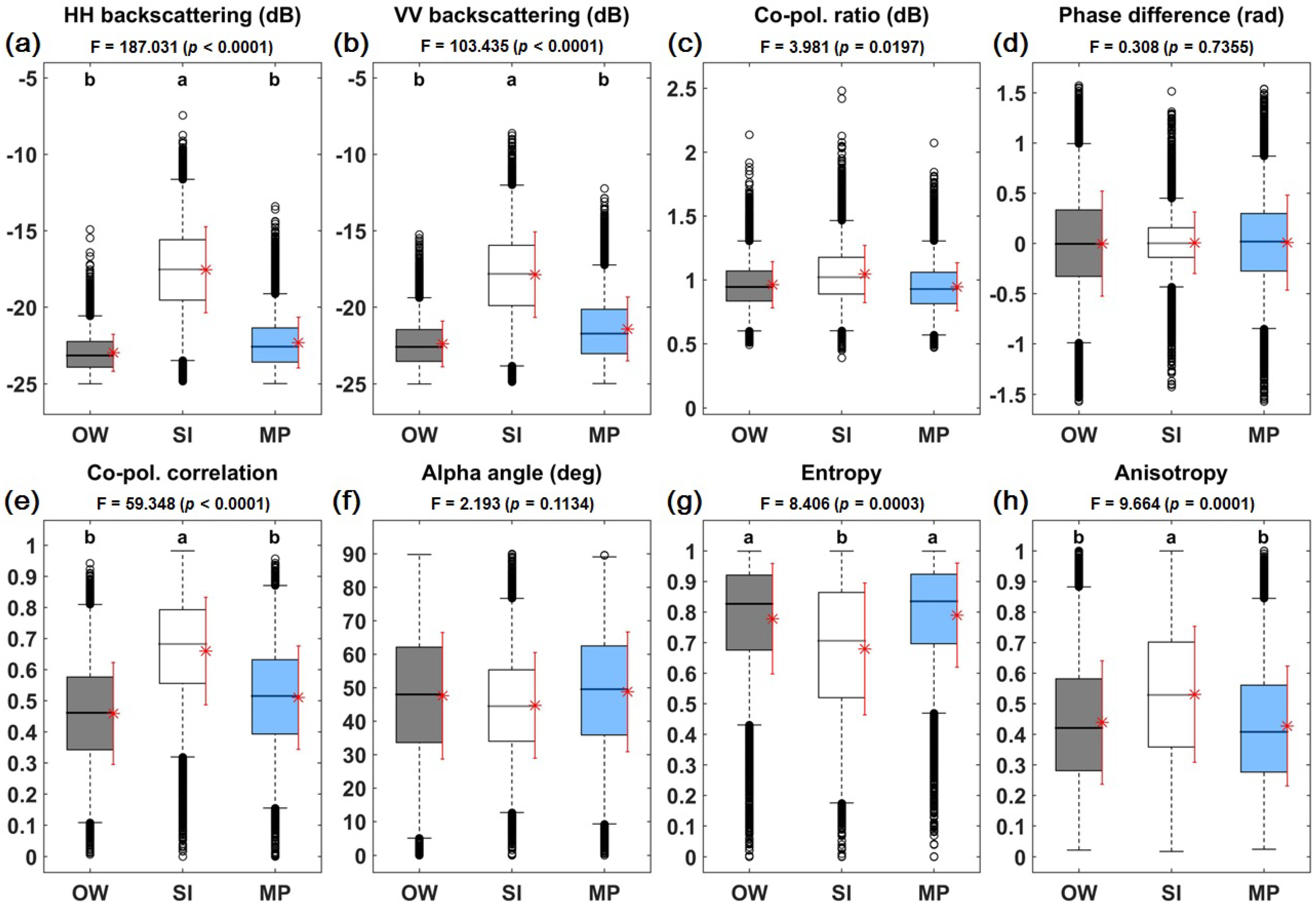
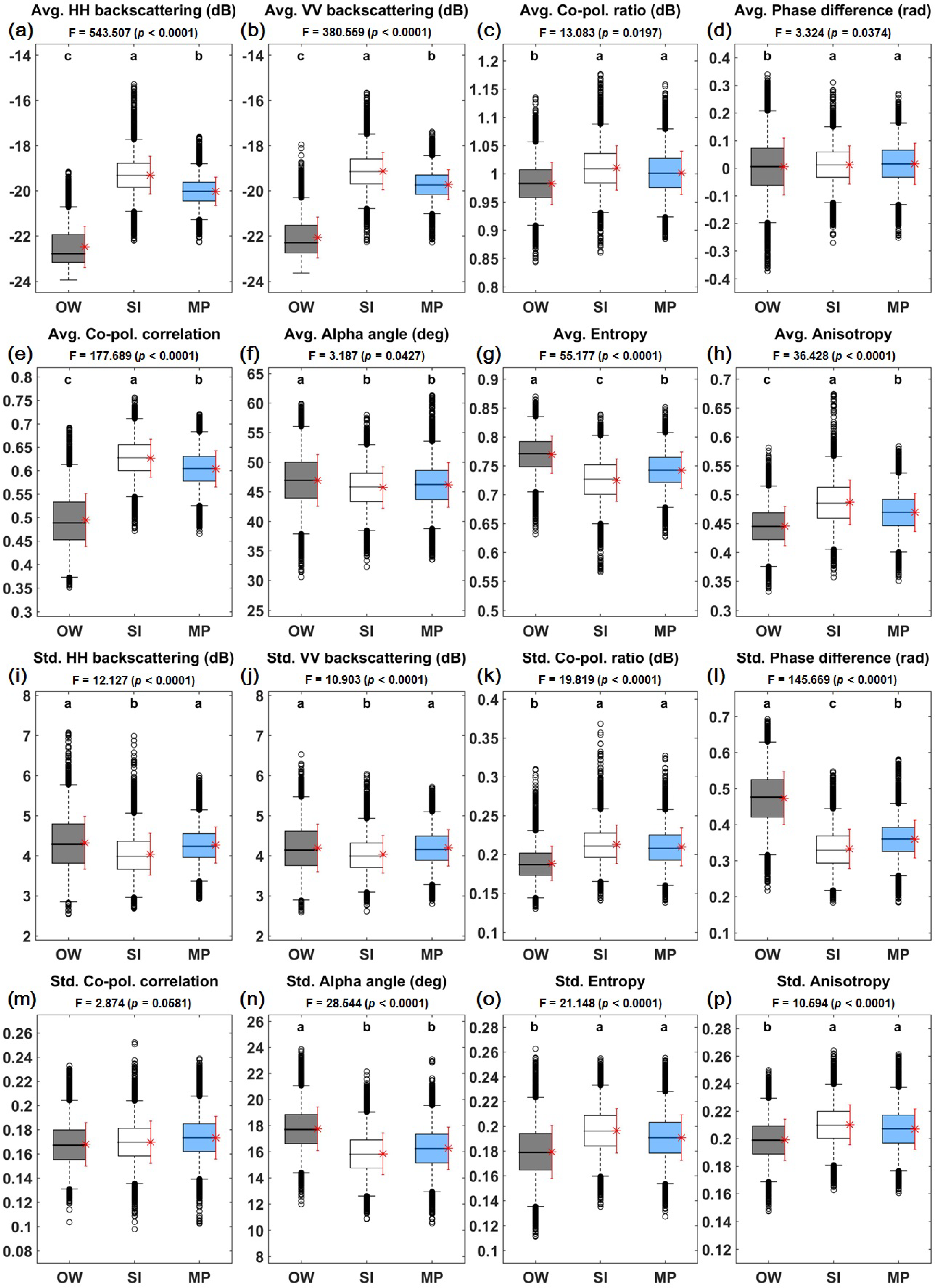
4.1. Polarimetric Signatures

The boxplots in Figure 3 show the characteristics of the polarimetric parameters in the samples of open water, sea ice and melt pond. The F-statistic and p-value in each boxplot were derived from the one-way analysis of variance (ANOVA) at the 95% confidence level. The p-values below 0.05 mean that at least one surface type can be distinguished from the other surface types by the polarimetric parameters. Tukey’s post hoc test at the 95% confidence level was carried out to identify which surface types can be discriminated from other surface types by a specific polarimetric parameter. The results of the post hoc tests are presented in each boxplot. Two surface types that cannot be discriminated from each other by the post hoc tests are denoted by the same lower case letter. The group names of the results of the post hoc tests are ordered according to the mean value of the samples. The ANOVA with post hoc tests was carried out using 300 randomly-selected samples (100 samples for each surface type) from a total of 37,152 samples (12,384 samples for each surface type), because the large sample size can overestimate the F-statistic, flagging the minute differences between the surface types as statistically significant. The sample size of 300 was determined by power analysis for one-way ANOVA with three groups conducted in G*Power [72] using an effect size of 0.25, an alpha of 0.05 and a power of 0.95.
Figure 3. Boxplots of the polarimetric parameters used for the melt pond retrieval: (a) backscattering coefficient at HH polarization; (b) backscattering coefficient at VV polarization; (c) co-polarization ratio; (d) co-polarization phase difference; (e) co-polarization correlation coefficient; (f) alpha angle, (g) entropy; and (h) anisotropy. Colored boxes represent the interquartile range of the samples, while a line inside the box means the median value of the samples. The vertical lines above and below the box represent 1.5-times the interquartile range beyond the lower and upper quartiles, and the dots represent the outliers. The red asterisks on the right side of boxes represent the mean value of the samples, while the red vertical lines above and below the asterisk mean the standard deviation of the samples. Co-pol, OW, SI, and MP indicate co-polarization, open water, sea ice, and melt pond, respectively.
Remotesensing 08 00057 g003
The boxplots in Figure 3 show that the values of the polarimetric parameters for sea ice (i.e., multiyear ice) are distinct from those for open water and melt ponds, except for the co-polarization ratio, the phase difference and the alpha angle, which showed a similar median value and interquartile range for all surface types. The values of HH and VV backscattering coefficients of sea ice were ~8 dB stronger than those of open water and melt ponds. This is because a sea ice surface is typically rougher than a calm open water surface [73,74]. The co-polarization correlation coefficient is close to one for an isotropic scattering medium (e.g., multiyear ice or snow), while it decreases when the scattering medium is anisotropic (e.g., new ice and first-year ice) or the backscattering coefficients are close to the noise level [35]. Sea ice in the study area was composed of multiyear ice floes and snow-covered first-year ice [28], which show larger values of the co-polarization correlation coefficient than open water and melt ponds, which show very low backscattering signals. The sea ice showed lower entropy values and larger anisotropy values than open water and melt ponds. This is possibly caused by the multiple scattering from the isotropic layer of multiyear ice floes and snow on the surface of first-year ice [75,76]. While multiyear ice can be identified from the polarimetric parameters, open water and melt ponds cannot be clearly distinguished from each other by the post hoc tests (Figure 3).

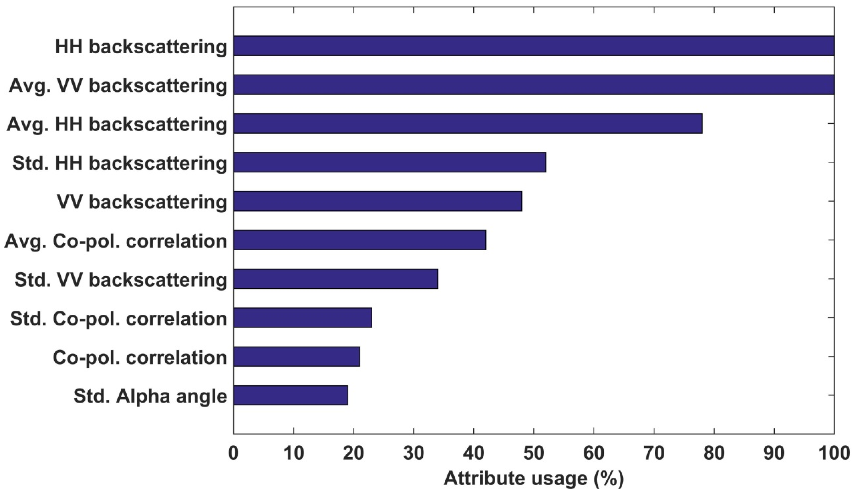
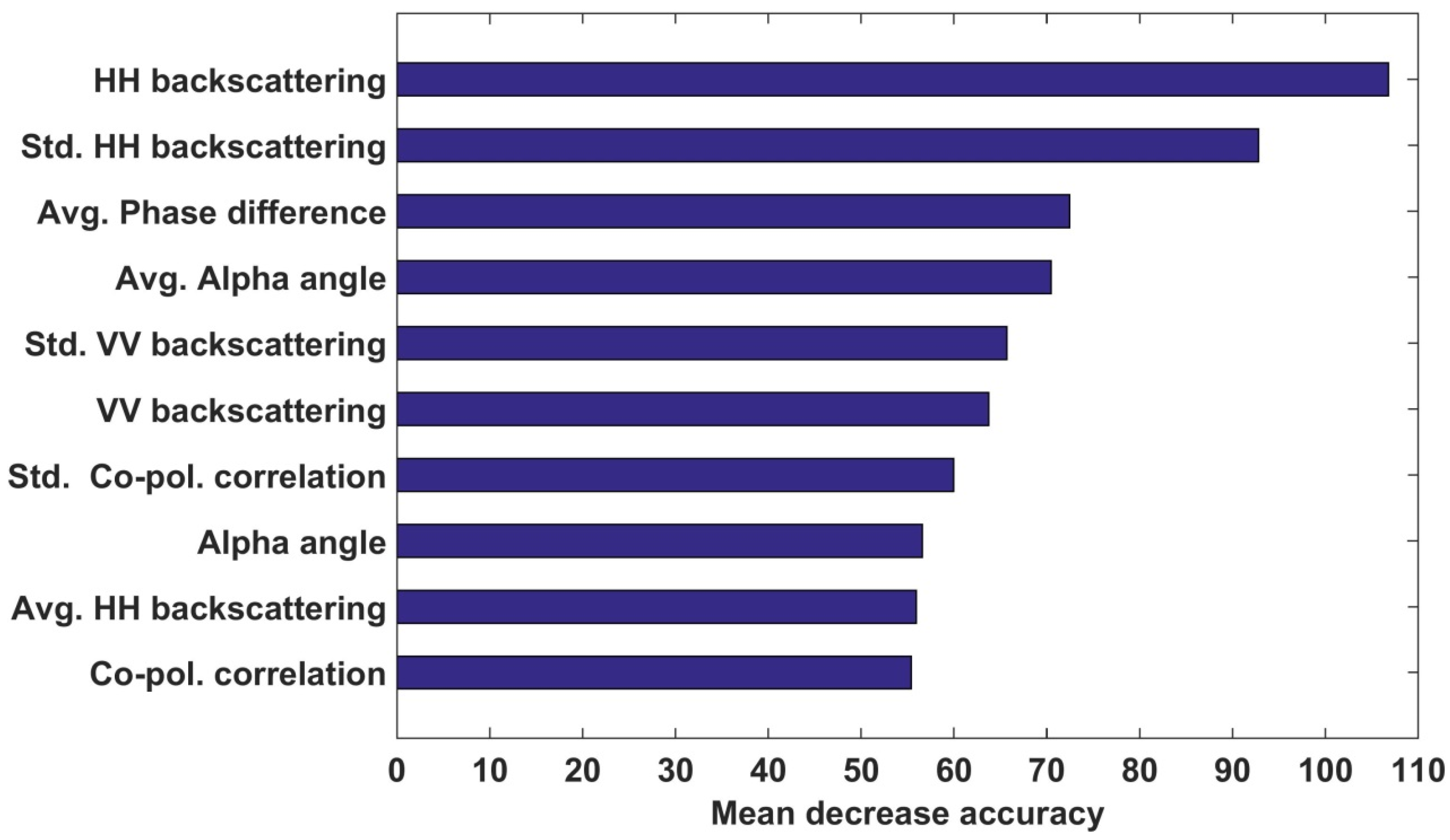
4.2. Performance of Melt Pond Detection Model Using Polarimetric Parameters

The test dataset was used to produce confusion matrices in order to assess the performance of the machine learning models developed using the polarimetric parameters. Both the DT and RF models showed relatively low overall accuracies of 66.56% and 69.88%, respectively, and low kappa coefficients of 49.89% and 54.82%, respectively (Table 1 and Table 2). The user’s and producer’s accuracies of sea ice were higher than 80% for both models, because multiyear ice floes showed distinctive polarimetric characteristics from open water and melt ponds. However, the user’s and producer’s accuracies of open water and melt pond on multiyear ice were very low for both models (Table 1 and Table 2) due to the similarity in the polarimetric characteristics between the two classes. This means that the polarimetric parameters might not be effective for the detection of melt ponds on multiyear ice and suggests the need for supplemental variables for discriminating melt ponds from open water.
Table 1. Accuracy assessment results for the DT model that was developed using the polarimetric parameters.
ReferenceOpen WaterSea IceMelt PondSumUser’s Accuracy
Classified as
Open water1865791197314159.38%
Sea ice542152349255584.23%
Melt pond558246931173553.66%
Sum2477247724777431
Producer’s accuracy75.29%86.88%37.59%
Overall accuracy66.59%
Kappa coefficient49.88%
Table 2. Accuracy assessment results for the RF model that was developed using the polarimetric parameters.
ReferenceOpen WaterSea IceMelt PondSumUser’s Accuracy
Classified as
Open water1955501175318061.48%
Sea ice272222286253587.65%
Melt pond4952051016171659.21%
Sum2477247724777431
Producer’s accuracy78.93%89.71%41.02%
Overall accuracy69.88%
Kappa coefficient54.82%
The melt ponds on multiyear ice and open water showed similar polarimetric characteristics, which resulted in the low performance of the machine learning models evaluated above. In order to discriminate the melt ponds from open water by the polarimetric characteristics, texture features of the polarimetric parameters can be used. Melt ponds on multiyear ice were typically less than 100 m2 [28], while open water formed in much larger areas than the melt ponds and contained few ice fragments. Therefore, within a pixel window larger than melt pond areas, the texture features of a polarimetric parameter computed for the window of which the center is a melt pond can be distinct from those of open water due to the difference of the spatial homogeneity. The average values of the polarimetric parameters within a pixel window for melt ponds would be different from those for sea ice and open water. The standard deviation values of the polarimetric parameters for melt ponds are expected to be larger than those for sea ice and open water. The texture features of the polarimetric parameters can be supplementary to the variables of the machine learning models, which might improve the performance of the retrieval of melt ponds on multiyear ice floes.

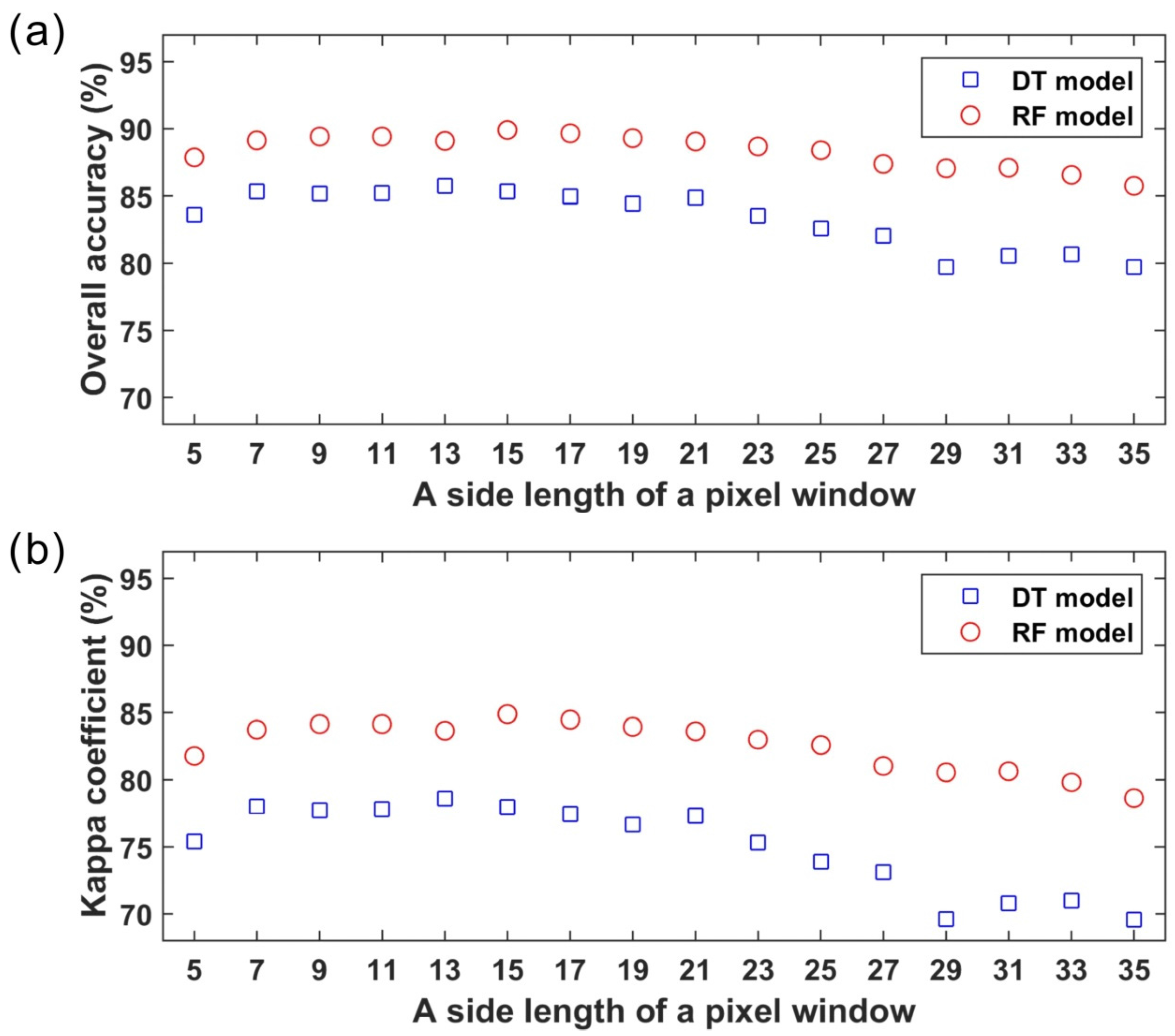
4.3. Performance of the Melt Pond Detection Model Considering the Texture Features of the Polarimetric Parameters

The texture features of the polarimetric parameters were calculated based on a pixel window in a square with a side length ranging from 5–35 pixels of the TerraSAR-X data obtained in a mid-incidence angle (32.7°) and used as the additional input variables for the machine learning models. The overall accuracies and kappa coefficients for the machine learning models were derived from confusion matrices using the test samples (Figure 4) and then assessed in order to find an optimum pixel window for calculating the texture features. The overall performance of the machine learning models was improved, compared to the previously-developed models that used only the polarimetric parameters (Table 1 and Table 2). The DT and RF models showed the highest overall performance when adopting the texture features of the polarimetric parameters based on 13 × 13 and 15 × 15 pixel windows, respectively. The RF models showed higher overall accuracies (85.7%–89.9%) and kappa coefficients (78.6%–84.9%) than the DT models (79.7%–85.7% and 69.6%–78.6%, respectively). The overall accuracy and kappa coefficient produced from the DT model adopting the texture features based on a 15 × 15 pixel window were only 0.7% lower than the best DT model that uses the texture features based on a 13 × 13 pixel window. Therefore, a 15 × 15 pixel window was selected as the optimum window for computing the texture features of the polarimetric parameters.
Figure 4. The variations of the overall accuracy and the kappa coefficient for the DT and RF model that were developed using the polarimetric parameters and their texture features based on a pixel window, ranging from 5–35: (a) the variations of the overall accuracies; and (b) the variations of the kappa coefficients.
Remotesensing 08 00057 g004
Figure 5 shows the boxplots of the texture features of the polarimetric parameters based on a 15 × 15 pixel window using the samples of open water, sea ice and melt pond. The ANOVA with Tukey’s post hoc test at the 95% confidence level was performed for each variable. The melt ponds on multiyear ice were statistically discriminated from the open water and sea ice using the average of the HH and VV backscattering coefficients, the co-polarization correlation, the co-polarization phase difference, the alpha angle, the entropy, the anisotropy and the standard deviation of the phase difference. The other variables of the texture features for melt ponds and open water showed similar mean values.
Figure 5. Boxplots of the texture features of the polarimetric parameters used as the supplementary variables for melt pond retrieval: (ah) the average of the polarimetric parameters based on a 15 × 15 pixel window; and (ip) the standard deviation of the polarimetric parameters based on a 15 × 15 pixel window. Co-pol, Avg, and Std indicate co-polarization, average, and standard deviation, respectively.
Remotesensing 08 00057 g005
The confusion matrices of the DT and RF models developed using the polarimetric parameters and their texture features based on a 15 × 15 pixel window are presented in Table 3 and Table 4, respectively. Both models showed a much improved classification performance, especially for melt ponds and open water, compared to the models developed using only the polarimetric parameters. The overall accuracy and the kappa coefficient of the RF model (90.05% and 85.12%) were higher than the DT model (85.33% and 78.0%). The user’s and producer’s accuracies for the open water, sea ice and melt pond were also higher in the RF model than the DT model, which is possibly due to a superior categorization strategy of RF [48,63].
Table 3. Accuracy assessment results for the DT model that was developed using the polarimetric parameters and their texture features.
ReferenceOpen WaterSea IceMelt PondSumUser’s Accuracy
Classified as
Open water233314210255791.24%
Sea ice152175434262482.89%
Melt pond1292881833225081.47%
Sum2477247724777431
Producer’s accuracy94.19%87.81%74.0%
Overall accuracy85.33%
Kappa coefficient78.0%
Table 4. Accuracy assessment results for the RF model that was developed using the polarimetric parameters and their texture features.
ReferenceOpen WaterSea IceMelt PondSumUser’s Accuracy
Classified as
Open water23667125249894.72%
Sea ice52280304258988.06%
Melt pond1061902048234487.37%
Sum2477247724777431
Producer’s accuracy95.52%92.04%82.68%
Overall accuracy90.08%
Kappa coefficient85.12%
The relative importance of the variables ranked in the top 10 most important variables for the DT and RF models is shown in Figure 6 and Figure 7, respectively. The HH backscattering coefficient was used as the most important variable in both models. The HH backscattering coefficient would be used for the discrimination of sea ice from open water and melt ponds based on the difference of surface roughness under low wind speed conditions [73,74]. In the DT model, the average of the VV backscattering coefficients was also used as the most important variable, and the average of the HH backscattering coefficients was the next important one (Figure 6). The melt pond samples of the average of the backscattering coefficients showed much higher values than the open water samples due to the strong backscattering signals from the surrounding sea ice, but smaller values than sea ice samples (Figure 5). Therefore, the average of the backscattering coefficients in a mid-incidence angle would contribute to the distinction between melt ponds on multiyear ice and open water. The standard deviation of the HH backscattering coefficients in a mid-incidence angle was identified as the second important variable in the RF model (Figure 7), which would contribute to separation of sea ice from open water and melt ponds. The average of the co-polarization phase difference and the alpha angle in a mid-incidence angle were also identified as the important variables in the RF model, which was possibly used in order to distinguish melt ponds on multiyear ice from open water. The average of the co-polarization correlation, entropy and anisotropy and the standard deviation of the phase difference in a mid-incidence angle showed a significant difference between melt ponds and other surface types, but their contributions to the machine learning models were relatively low. This would be because the melt pond samples showed much more distinct characteristics from open water for the texture features of the HH and VV backscattering coefficients compared to other input variables derived in a mid-incidence angle (Figure 5).
Figure 6. Attribute usage of the DT model that was developed using the polarimetric parameters and their texture features based on a 15 × 15 pixel window.
Remotesensing 08 00057 g006
Figure 7. Mean decrease accuracy of the RF model that was developed using the polarimetric parameters and their texture features based on a 15 × 15 pixel window.
Remotesensing 08 00057 g007
Melt pond mapping results from the DT and RF models were compared to the melt pond maps derived from the airborne SAR images. Figure 8 shows a comparison between a reference melt pond map and machine learning results. The open water areas detected by both models were well matched to those from the airborne SAR image. However, the DT model overestimated melt pond areas and underestimated sea ice areas compared to the melt pond map from the airborne SAR image. The RF model detected the areas of melt ponds and sea ice better than the DT model, which may be because the bootstrapping and ensemble strategies of the RF model overcome the problems of overfitting that is the limitation of the DT model [66,67,77].
Since the RF-based melt pond retrieval model using the polarimetric parameters and their texture features based on a 15 × 15 pixel window performed better than the other machine learning models, it was applied to the TerraSAR-X dual polarization data obtained on 21 July 2010. As there was no reference data of melt ponds available over the area of the 2010 TerraSAR-X swath, the melt pond mapping result of the RF model was visually assessed in comparison to the amplitude image. Figure 9 shows comparisons between the amplitude images and melt pond mapping results. The melt ponds and open water detected from the RF model showed close agreement with dark areas observed in the amplitude images. The RF model detected most of the dark and small areas as melt ponds, with discrimination of large and dark areas as open water. Some melt ponds were identified by the model in dark areas of a large size, which appeared as open water (yellow circles in Figure 9). Although it is not clear whether the large and dark areas of the amplitude images are actual open water, it might be possible to say that the RF model did not produce as high performance for melt pond retrievals from the 2010 TerraSAR-X data as that from the 2011 ones, because it would be biased to the 2011 TerraSAR-X data and might not work well for the different sea ice and weather conditions.
Figure 8. The comparison between (a) the airborne SAR- and machine learning results-based melt pond maps: (b) the DT model and (c) the RF model.
Remotesensing 08 00057 g008
Figure 9. Visual comparisons between the 2010 TerraSAR-X HH-polarized amplitude images (a,b) and the RF model-based melt pond maps (c,d).
Remotesensing 08 00057 g009

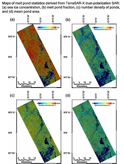
4.4. Retrieved Melt Pond Statistics

As the RF model produced better classification results than the DT model, the RF-derived melt pond map was used to obtain the statistics for melt ponds. The root mean square deviation (RMSD) between the sea ice concentration produced from the airborne SAR-derived maps and the RF-derived map was only 4.9% (a normalized RMSD (NRMSD) of 7.7%) (Figure 10a), which resulted from the high performance of the RF model for discriminating sea ice from open water and melt ponds. The melt pond fractions estimated from the RF-derived map were similar to those from the airborne SAR images (Figure 10b), with an RMSD of 2.4% (an NRMSD of 15.8%). The number density of melt ponds retrieved from the RF-derived map and the airborne SAR images showed an NRMSD of 17.4% (Figure 10c), which is similar to the NRMSD for the melt pond fraction (Figure 10b). However, the range of the number density retrieved from the RF-derived map (1500–2867 km−2) was much smaller than that from the airborne SAR images (1061–3808 km−2), which was clearly attributed to the lower spatial resolution of the TerraSAR-X dual-polarimetric data (3 m) than the airborne SAR data (0.3 m). The melt ponds with a narrow width could not be detected in the RF model, even though the pond areas are larger than 9 m2 due to the spatial resolution of the TerraSAR-X data. The mean pond area retrieved from the RF-derived map showed a relatively large NRMSD (23.9%) compared to that from the airborne SAR-derived melt pond maps (Figure 10d). Such a large deviation can be attributed to the difference of the spatial resolutions between the TerraSAR-X and airborne SAR data.
Figure 10. The comparison between the airborne SAR- and the RF model-derived statistics for melt pond and sea ice: (a) sea ice concentration; (b) melt pond fraction; (c) number density of ponds and (d) mean pond area. NRMSD, normalized RMSD.
Remotesensing 08 00057 g010
The comparison results indicate that the high-resolution dual-polarimetric parameters and their texture features have potential to provide the reliable estimation of melt pond fraction and sea ice concentration in the summer melting peak season of the Arctic sea ice based on the RF approach. However, the RF-derived melt pond map could not estimate the number density or mean pond area accurately due to the existence of small and narrow melt ponds.
The statistics for melt ponds were computed for a 50 by 50 pixel window of the 2011 TerraSAR-X data using the RF-derived melt pond map and gridded at a 150-m grid size (Figure 11). The values of sea ice concentration were close to 100% in the areas of the multiyear ice floes, while less than 90% in the areas of the heavily-melted ice fragments (Figure 11a). The melt pond fractions on the heavily-melted ice fragments were less than 10%, while those on the multiyear ice floes varied from 10%–28% (Figure 11b). The higher melt pond fractions on the multiyear ice floes were attributed to a larger fraction of ice [28]. The number density and the mean area of melt ponds were estimated as ~3800 km−2 (Figure 11c) and ~120 m2 (Figure 11d), respectively, in the areas of both the multiyear ice floes and heavily-melted ice fragments. However, again, note that the number density and mean pond area obtained by the RF model would be inaccurate, because the narrow and small melt ponds (less than 9 m2 in size) would not be detected due to the spatial resolution of the TerraSAR-X data.
Figure 11. Maps of the statistics for melt pond and sea ice generated from the RF model-derived melt pond map: (a) sea ice concentration; (b) melt pond fraction; (c) number density of ponds; and (d) mean pond area.
Remotesensing 08 00057 g011
Kim et al. [28] estimated melt pond fraction by mapping ponds from the same TerraSAR-X data based on the combination of multiscale segmentation and aggregation of the amplitude image. They reported that the melt pond fraction derived by their methodology was significantly underestimated compared to the airborne SAR survey. This implies that the use of the single-polarized backscattering amplitude only might not be sufficient for retrieval of the ponds. Since the RF model in the present study was developed using various polarimetric parameters and their texture features, which provided more abundant information to discriminate melt ponds from sea ice and open water, it was able to provide a more accurate melt pond fraction.
The machine learning models were developed and assessed using only two mid-incidence angle (32.7°) TerraSAR-X dual polarization images of very small swath widths for the summer multiyear ice floes in the Chukchi Sea. The characteristics of the polarimetric parameters for sea ice and melt ponds can change significantly with ice conditions, wind speed and incidence angles [32,34,78]. In particular, the texture features of polarimetric parameters used in the machine learning models are second order statistics, which would change significantly with the variation of incidence angles. Therefore, the melt pond retrieval models developed in this study can be applied to the X-band dual polarization SAR data of a small swath width with mid-incidence angle for detecting melt ponds on multiyear ice in the summer season, but cannot be directly used for other incidence angle data containing other sea ice types in wide areas. In order to develop a general-purpose melt pond retrieval model, it is required to use a number of polarimetric SAR data for various sea ice types with different incidence angles and to construct sufficient reference datasets corresponding to the SAR data. Furthermore, an artificial neural network approach using the texture features of polarimetric parameters is needed to be evaluated for melt pond retrievals, because it might be useful for texture-based classification [79].
The machine learning-based classification of high-resolution dual-polarization X-band SAR data with the mid-incidence angle (32.7°) shows potential to accurately estimate the melt pond fraction on the summer multiyear sea ice in the Chukchi Sea. The proposed models for melt pond detection are only applicable to situations where individual melt ponds are larger than the pixel size of SAR data, which is an important distinction from the previous studies that developed techniques for unmixing the melt pond fraction from mixed pixels [17,32]. The TerraSAR-X dual-polarization data can be effectively used for regular monitoring of the melt pond fraction on a local scale (typically less than 100 km2) based on the revisit time of the satellite, but not enough to observe melt ponds at a regional scale due to the limitation of the swath of the polarimetric SAR data. In order to study the relationship between sea ice ponding and climate change, the melt pond fractions at a much larger spatial scale should be monitored. Satellite optical data, such as MODIS and MERIS, can be used to retrieve the melt pond fraction over a regional scale [17,19,21,22]. However, the prevailing cloudy days in the summer season make it difficult to observe melt ponds using optical data. Passive microwave sensors can be used for monitoring melt ponds in the entire Arctic regardless of cloud conditions because the microwave emissivity of sea ice can vary by the fraction of melt ponds [5,11,80,81].

5. Conclusions

Melt ponds on summer multiyear sea ice in the Chukchi Sea in the Arctic were retrieved using the classification of two TerraSAR-X dual co-polarization data with the mid-incidence angle (32.7°) obtained in July 2010 and August 2011, respectively, based on two machine learning approaches—DT and RF. The reference dataset for the classification of melt ponds, sea ice and open water was constructed from the airborne SAR images obtained coincident with the TerraSAR-X data acquisition in 2011. The machine learning models using only the polarimetric parameters could not discriminate melt ponds on multiyear ice from open water due to their similar polarimetric signatures, while those using the polarimetric parameters and their spatial average and standard deviation based on a 15 × 15 pixel window showed much improved performance for the melt pond retrieval. The RF model produced better performance for retrieving melt ponds than the DT model based on the accuracy assessment. The HH backscattering coefficient, its spatial standard deviation and the average of the co-polarization phase differences and the alpha angles were defined as more contributing variables than the other ones by the RF model. The RF-derived melt pond mapping result from the TerraSAR-X data obtained in 2010 was compared to the dark areas observed in the amplitude image due to lack of reference data. The RF model identified most of the small and dark areas as melt ponds. Melt pond statistics for the 2011 TerraSAR-X data were calculated from the RF-derived melt pond map. The melt pond fraction and sea ice concentration estimated from the RF-derived melt pond map showed RMSDs of 2.4% and 4.9%, respectively, compared to the airborne SAR-derived maps. This means that there is potential to accurately retrieve melt pond fraction and sea ice concentration for multiyear ice in the Arctic summer season from high-resolution mid-incidence angle dual-polarization SAR data. However, the melt pond retrieval models would not be enough to estimate the number density of ponds and mean pond area because of the melt ponds being smaller than the pixel size of the TerraSAR-X data.
The melt pond retrieval models proposed in this study could not be validated for different ice types and incidence angles. The swath of the TerraSAR-X dual-polarization imaging mode is not enough to observe melt ponds on wide-area sea ice. Future research includes: (1) developing pond fraction retrieval models using multi-polarization SAR data in different incidence angles for various ice types and in situ observations of the ponds based on icebreakers; (2) studying the relationship between the polarimetric signatures and microwave emissivity of melt ponds; and (3) monitoring melt pond fractions over the entire Arctic using the ensemble of multi-polarization SAR data and passive microwave observations.

Acknowledgments

This research was a part of the project titled “Korea-Polar Ocean in Rapid Transition (KOPRI, PM15040)”, funded by the Ministry of Oceans and Fisheries, Korea. The TerraSAR-X dataset was provided by the German Aerospace Center (DLR).

Author Contributions

Hyangsun Han led manuscript writing and contributed to the data analysis and research design. Jungho Im supervised this study, contributed to the research design and manuscript writing and served as the corresponding author. Miae Kim contributed to the data analysis and discussion of the results. Sungmoon Sim contributed to data processing and analysis. Jinwoo Kim and Duk-jin Kim provided SAR data and contributed to the discussion of the results and manuscript writing. Sung-Ho Kang contributed to the discussion of the results and manuscript writing.

Conflicts of Interest

The authors declare that there are no conflicts of interest.

References

  1. Cavalieri, D.J.; Parkinson, C.L. Arctic sea ice variability and trends, 1979–2010. Cryosphere 2012, 6, 881–889. [Google Scholar] [CrossRef]
  2. Comiso, J.C. Large decadal decline of the arctic multiyear ice cover. J. Clim. 2012, 25, 1176–1193. [Google Scholar] [CrossRef]
  3. Kay, J.E.; Holland, M.M.; Jahn, A. Inter-annual to multi-decadal Arctic sea ice extent trends in a warming world. Geophys. Res. Lett. 2011. [Google Scholar] [CrossRef]
  4. Screen, J.A.; Deser, C.; Simmonds, I.; Tomas, R. Atmospheric impacts of Arctic sea-ice loss, 1979–2009: Separating forced change from atmospheric internal variability. Clim. Dyn. 2014, 43, 333–344. [Google Scholar] [CrossRef] [Green Version]
  5. Stroeve, J.C.; Kattsov, V.; Barrett, A.; Serreze, M.; Pavlova, T.; Holland, M.; Meier, W.N. Trends in Arctic sea ice extent from CMIP5, CMIP3 and observations. Geophys. Res. Lett. 2012. [Google Scholar] [CrossRef]
  6. Vihma, T. Effects of Arctic sea ice decline on weather and climate: A review. Surv. Geophys. 2014, 35, 1175–1214. [Google Scholar] [CrossRef]
  7. Francis, J.A.; Vavrus, S.J. Evidence linking Arctic amplification to extreme weather in mid-latitudes. Geophys. Res. Lett. 2012. [Google Scholar] [CrossRef]
  8. Gautier, D.L.; Bird, K.J.; Charpentier, R.R.; Grantz, A.; Houseknecht, D.W.; Klett, T.R.; Moore, T.E.; Pitman, J.K.; Schenk, C.J.; Schuenemeyer, J.H.; et al. Assessment of undiscovered oil and gas in the Arctic. Science 2009, 324, 1175–1179. [Google Scholar] [CrossRef] [PubMed]
  9. Hansen, B.B.; Grøtan, V.; Aanes, A.; Sæther, B.-E.; Stien, A.; Fuglei, E.; Ims, R.A.; Yoccoz, N.G.; Pedersen, Å.Ø. Climate events synchronize the dynamics of a resident vertebrate community in the high Arctic. Science 2013, 339, 313–315. [Google Scholar] [CrossRef] [PubMed]
  10. Eicken, H.; Grenfell, T.C.; Perovich, D.K.; Richter-Menge, J.A.; Frey, K. Hydraulic controls of summer Arctic pack ice albedo. J. Geophys. Res. 2004. [Google Scholar] [CrossRef]
  11. Fetterer, F.; Untersteiner, N. Observations of melt ponds on Arctic sea ice. J. Geophys. Res. 1998, 103, 24821–24835. [Google Scholar] [CrossRef]
  12. Perovich, D.K.; Grenfell, T.C.; Light, B.; Hobbs, P.V. Seasonal evolution of the albedo of multiyear Arctic sea ice. J. Geophys. Res. 2002, 107, SHE 20-1–SHE 20-13. [Google Scholar] [CrossRef]
  13. Perovich, D.K.; Richter-Menge, J.A.; Jones, K.F.; Light, B. Sunlight, water, and ice: Extreme Arctic sea ice melt during the summer of 2007. Geophys. Res. Lett. 2008, 35, L11501. [Google Scholar] [CrossRef]
  14. Perovich, D.K.; Tucker, W.B., III; Ligett, K.A. Aerial observations of the evolution of ice surface conditions during summer. J. Geophys. Res. 2002, 107, 194–198. [Google Scholar]
  15. Flocco, D.; Feltham, D.L.; Turner, A.K. Incorporation of a physically based melt pond scheme into the sea ice component of a climate model. J. Geophys. Res. 2010, 115, 488–507. [Google Scholar] [CrossRef]
  16. Schröder, D.; Feltham, D.L.; Flocco, D.; Tsamados, M. September Arctic sea-ice minimum predicted by spring melt-pond fraction. Nat. Clim. Chang. 2014, 4, 353–357. [Google Scholar] [CrossRef]
  17. Istomina, L.; Heygster, G.; Huntemann, M.; Schwarz, P.; Birnbaum, G.; Scharien, R.; Polashenski, C.; Perovich, D.; Zege, E.; Malinka, A.; et al. Melt pond fraction and spectral sea ice albedo retrieval from MERIS data—Part 1: Validation against in situ, aerial, and ship cruise data. Cryosphere 2015, 9, 1551–1566. [Google Scholar] [CrossRef] [Green Version]
  18. Markus, T.; Cavalieri, D.J.; Tschudi, M.A.; Ivanoff, A. Comparison of aerial video and Landsat 7 data over ponded sea ice. Remote Sens. Environ. 2003, 86, 458–469. [Google Scholar] [CrossRef]
  19. Rösel, A.; Kaleschke, L. Comparison of different retrieval techniques for melt ponds on Arctic sea ice from Landsat and MODIS satellite data. Ann. Glaciol. 2011, 52, 185–191. [Google Scholar] [CrossRef]
  20. Rösel, A.; Kaleschke, L. Exceptional melt pond occurrence in the years 2007 and 2011 on the Arctic sea ice revealed from MODIS satellite data. J. Geophys. Res. 2012, 117, 78–91. [Google Scholar] [CrossRef]
  21. Rösel, A.; Kaleschke, L.; Birnbaum, G. Melt ponds on Arctic sea ice determined from MODIS satellite data using an artificial neural network. Cryosphere 2012, 6, 431–446. [Google Scholar] [CrossRef] [Green Version]
  22. Tschudi, M.A.; Maslanik, J.A.; Perovich, D.K. Derivation of melt pond coverage on Arctic sea ice using MODIS observations. Remote Sens. Environ. 2008, 112, 2605–2614. [Google Scholar] [CrossRef]
  23. Zege, E.; Malinka, A.; Katsev, I.; Prikhach, A.; Heygster, G.; Istomina, L.; Birnbaum, G.; Schwarz, P. Algorithm to retrieve the melt pond fraction and the spectral albedo of Arctic summer ice from satellite optical data. Remote Sens. Environ. 2015, 163, 153–164. [Google Scholar] [CrossRef] [Green Version]
  24. Liu, J.; Song, M.; Horton, R.M.; Hu, Y. Revisiting the potential of melt pond fraction as a predictor for the seasonal Arctic sea ice extent minimum. Environ. Res. Lett. 2015. [Google Scholar] [CrossRef]
  25. Lupkes, C.; Gryanik, V.M.; Rösel, A.; Birnbaum, G.; Kaleschke, L. Effect of sea ice morphology during Arctic summer on atmospheric drag coefficients used in climate models. Geophys. Res. Lett. 2013, 40, 446–451. [Google Scholar] [CrossRef]
  26. Yackel, J.J.; Barber, D.G. Melt ponds on sea ice in the Canadian Archipelago 2. On the use of RADARSAT-1 synthetic aperture radar for geophysical inversion. J. Geophys. Res. 2000, 105, 22061–22070. [Google Scholar] [CrossRef]
  27. Mäkynen, M.; Kern, S.; Rösel, A.; Pedersen, L.T. On the estimation of melt pond fraction on the Arctic sea ice with ENVISAT WSM images. IEEE Trans. Geosci. Remote Sens. 2014, 52, 7366–7379. [Google Scholar] [CrossRef]
  28. Kim, D.-J.; Hwang, B.; Chung, K.H.; Lee, S.H.; Jung, H.S.; Moon, W.M. Melt pond mapping with high-resolution SAR: The first view. Proc. IEEE 2013, 101, 748–758. [Google Scholar] [CrossRef]
  29. Mishra, P.; Singh, D. A statistical-measure-based adaptive land cover classification algorithm by efficient utilization of polarimetric SAR observables. IEEE Trans. Geosci. Remote Sens. 2014, 52, 2889–2900. [Google Scholar] [CrossRef]
  30. Sawaya, S.; Haack, B.; Idol, T.; Sheoran, A. Land use/cover mapping with quad-polarization radar and derived texture measures near Wad Madani, Sudan. GISci. Remote Sens. 2010, 47, 398–411. [Google Scholar] [CrossRef]
  31. Sheoran, A.; Haack, B. Classification of California agriculture using quad polarization radar data and Landsat Thematic Mapper data. GISci. Remote Sens. 2013, 50, 50–63. [Google Scholar]
  32. Scharien, R.K.; Landy, J.; Barber, D.G. First-year sea ice melt pond fraction estimation from dual-polarisation C-band SAR—Part 1: In situ observations. Cryosphere 2014, 8, 2147–2162. [Google Scholar] [CrossRef]
  33. Scharien, R.K.; Yackel, J.J.; Barber, D.G.; Asplin, M.; Gupta, M.; Isleifson, D. Geophysical controls on C band polarimetric backscatter from melt pond covered Arctic first-year sea ice: Assessment using high-resolution scatterometry. J. Geophys. Res. 2012. [Google Scholar] [CrossRef]
  34. Scharien, R.K.; Hochheim, K.; Landy, J.; Barber, D.G. First-year sea ice melt pond fraction estimation from dual-polarisation C-band SAR—Part 2: Scaling in situ to Radarsat-2. Cryosphere 2014, 8, 2163–2176. [Google Scholar] [CrossRef]
  35. Dierking, W.; Wesche, C. C-band radar polarimetry—Useful for detection of icebergs in sea ice? IEEE Trans. Geosci. Remote Sens. 2014, 52, 25–37. [Google Scholar] [CrossRef]
  36. Gill, J.P.S.; Yackel, J.J. Evaluation of C-band SAR polarimetric parameters for discrimination of first-year sea ice types. Can. J. Remote Sens. 2012, 38, 306–323. [Google Scholar] [CrossRef]
  37. Barber, D.G.; Yackel, J. The physical, radiative and microwave scattering characteristics of melt ponds on Arctic landfast sea ice. Int. J. Remote Sens. 1999, 20, 2069–2090. [Google Scholar] [CrossRef]
  38. Breit, H.; Fritz, T.; Balss, U.; Lachaise, M.; Niedermeier, A.; Vonavka, M. TerraSAR-X SAR processing and products. IEEE Trans. Geosci. Remote Sens. 2010, 48, 727–740. [Google Scholar] [CrossRef]
  39. Werninghaus, R.; Buckreuss, S. The TerraSAR-X mission and system design. IEEE Trans. Geosci. Remote Sens. 2010, 48, 606–614. [Google Scholar] [CrossRef] [Green Version]
  40. Lee, J.-S.; Grunes, M.R.; de Grandi, G. Polarimetric SAR speckle filtering and its implication for classification. IEEE Trans. Geosci. Remote Sens. 1999, 37, 2363–2373. [Google Scholar]
  41. Lee, J.-S.; Pottier, E. Polarimetric Radar Imaging: From Basics to Applications; CRC Press: Boca Raton, FL, USA, 2009. [Google Scholar]
  42. Cloude, S.R.; Pottier, E. An entropy based classification scheme for land applications of polarimetric SAR. IEEE Trans. Geosci. Remote Sens. 1997, 35, 68–78. [Google Scholar] [CrossRef]
  43. Niu, X.; Ban, Y. Multi-temporal RADARSAT-2 polarimetric SAR data for urban land-cover classification using an object-based support vector machine and a rule-based approach. Int. J. Remote Sens. 2013, 34, 1–26. [Google Scholar] [CrossRef]
  44. Lopez-Sanchez, J.M.; Vicente-Guijalba, F.; Ballester-Berman, J.D.; Cloude, S.R. Polarimetric response of rice fields at C-band: Analysis and phenology retrieval. IEEE Trans. Geosci. Remote Sens. 2014, 52, 2977–2993. [Google Scholar] [CrossRef]
  45. Cloude, S.R. The dual polarization entropy/alpha decomposition: A PALSAR case study. In Proceedings of the 3rd International Workshop on Science and Applications of SAR Polarimetry and Polarimetric Interferometry, Frascati, Italy, 22–26 January 2007.
  46. Duro, D.C.; Franklin, S.E.; Dubé, M.G. A comparison of pixel-based and object-based image analysis with selected machine learning algorithms for the classification of agricultural landscapes using SPOT-5 HRG imagery. Remote Sens. Environ. 2012, 118, 259–272. [Google Scholar] [CrossRef]
  47. Ghimire, B.; Rogan, J.; Galiano, V.R.; Panday, P.; Neeti, N. An evaluation of bagging, boosting, and random forests for land-cover classification in Cape Cod, Massachusetts, USA. GISci. Remote Sens. 2012, 49, 623–643. [Google Scholar] [CrossRef]
  48. Kim, M.; Im, J.; Han, H.; Kim, J.; Lee, S.; Shin, M.; Kim, H.-C. Landfast sea ice monitoring using multisensor fusion in the Antarctic. GISci. Remote Sens. 2015, 52, 239–256. [Google Scholar] [CrossRef]
  49. Long, J.A.; Lawrence, R.L.; Greenwood, M.C.; Marshall, L.; Miller, P.R. Object-oriented crop classification using multitemporal ETM+ SLC-off imagery and random forest. GISci. Remote Sens. 2013, 50, 418–436. [Google Scholar]
  50. Maxwell, A.E.; Strager, M.P.; Warner, T.A.; Zégre, N.P.; Yuill, C.B. Comparison of NAIP orthophotography and RapidEye satellite imagery for mapping of mining and mine reclamation. GISci. Remote Sens. 2014, 51, 301–320. [Google Scholar] [CrossRef]
  51. Qian, Y.; Zhou, W.; Yan, J.; Li, W.; Han, L. Comparing machine learning classifiers for object-based land cover classification using very high resolution imagery. Remote Sens. 2014, 7, 153–168. [Google Scholar] [CrossRef]
  52. Rhee, J.; Park, S.; Lu, Z. Relationship between land cover patterns and surface temperature in urban areas. GISci. Remote Sens. 2014, 51, 521–536. [Google Scholar] [CrossRef]
  53. Demir, B.; Bovolo, F.; Bruzzone, L. Updating land-cover maps by classification of image time series: A novel change-detection-driven transfer learning approach. IEEE Trans. Geosci. Remote Sens. 2013, 51, 300–312. [Google Scholar] [CrossRef]
  54. Tan, B.; Masek, J.G.; Wolfe, R.; Gao, F.; Huang, C.; Vermote, E.F.; Sexton, J.O.; Ederer, G. Improved forest change detection with terrain illumination corrected Landsat images. Remote Sens. Environ. 2013, 136, 469–483. [Google Scholar] [CrossRef]
  55. Abedi, M.; Norouzi, G.-H.; Bahroudi, A. Support vector machine for multi-classification of mineral prospectivity areas. Comput. Geosci. 2012, 46, 272–283. [Google Scholar] [CrossRef]
  56. Li, M.; Im, J.; Beier, C. Machine learning approaches for forest classification and change analysis using multi-temporal Landsat TM images over Huntington Wildlife Forest. GISci. Remote Sens. 2013, 50, 361–384. [Google Scholar]
  57. Lu, D.; Li, G.; Moran, E.; Kuang, W. A comparative analysis of approaches for successional vegetation classification in the Brazilian Amazon. GISci. Remote Sens. 2014, 51, 695–709. [Google Scholar] [CrossRef]
  58. Xun, L.; Wang, L. An object-based SVM method incorporating optimal segmentation scale estimation using Bhattacharyya Distance for mapping salt cedar (Tamarisk spp.) with QuickBird imagery. GISci. Remote Sens. 2015, 52, 257–273. [Google Scholar] [CrossRef]
  59. Zhang, C.; Xie, Z.; Selch, D. Fusing lidar and digital aerial photography for object-based forest mapping in the Florida Everglades. GISci. Remote Sens. 2013, 50, 562–573. [Google Scholar]
  60. Ahmad, S.; Kalra, A.; Stephen, H. Estimating soil moisture using remote sensing data: A machine learning approach. Adv. Water Resour. 2010, 33, 69–80. [Google Scholar] [CrossRef]
  61. Güneralp, I.; Filippi, A.M.; Hales, B.U. River-flow boundary delineation from digital aerial photography and ancillary images using support vector machines. GISci. Remote Sens. 2013, 50, 1–25. [Google Scholar]
  62. Kim, Y.H.; Im, J.; Ha, H.K.; Choi, J.K.; Ha, S. Machine learning approaches to coastal water quality monitoring using GOCI satellite data. GISci. Remote Sens. 2014, 51, 158–174. [Google Scholar] [CrossRef]
  63. Han, H.; Lee, S.; Im, J.; Kim, M.; Lee, M.-I.; Ahn, M.H.; Chung, S.-R. Detection of convective initiation using Meteorological Imager onboard Communication, Ocean, and Meteorological satellite based on machine learning approaches. Remote Sens. 2015, 7, 9184–9204. [Google Scholar] [CrossRef]
  64. Kühnlein, M.; Appelhans, T.; Thies, B.; Nauss, T. Improving the accuracy of rainfall rates from optical satellite sensors with machine learning—A random forests-based approach applied to MSG SEVIRI. Remote Sens. Environ. 2014, 141, 129–143. [Google Scholar] [CrossRef]
  65. Quinlan, J.R. Data Mining Tools See5 and C4.5, Version 2.10. Available online: http://www.webcitation.org/6YgqVwnT9 (accessed on 9 September 2015).
  66. Breiman, L. Random forests. Mach. Learn. 2001, 45, 5–32. [Google Scholar] [CrossRef]
  67. Lawrence, R.L.; Wright, A. Rule-based classification systems using classification and regression tree (CART) analysis. Photogramm. Eng. Remote Sens. 2001, 67, 1137–1142. [Google Scholar]
  68. Cracknell, M.J.; Reading, A.M. Geological mapping using remote sensing data: A comparison of five machine learning algorithms, their response to variations in the spatial distribution of training data and the use of explicit spatial information. Comput. Geosci. 2014, 63, 22–33. [Google Scholar] [CrossRef]
  69. Congalton, R.G. A review of assessing the accuracy of classifications of remotely sensed data. Remote Sens. Environ. 1991, 37, 35–46. [Google Scholar] [CrossRef]
  70. Foody, G.M. Status of land cover classification accuracy assessment. Remote Sens. Environ. 2002, 80, 185–201. [Google Scholar] [CrossRef]
  71. Stehman, S.V. Selecting and interpreting measures of thematic classification accuracy. Remote Sens. Environ. 1997, 62, 77–89. [Google Scholar] [CrossRef]
  72. Faul, F.; Erdfelder, E.; Lang, A.-G.; Buchner, A. G*power 3: A flexible statistical power analysis program for the social, behavioral, and biomedical sciences. Behav. Res. Methods 2007, 39, 175–191. [Google Scholar] [CrossRef] [PubMed]
  73. Deng, H.; Clausi, D.A. Unsupervised segmentation of synthetic aperture radar sea ice imagery using a novel Markov random field model. IEEE Trans. Geosci. Remote Sens. 2005, 43, 528–538. [Google Scholar] [CrossRef]
  74. Liu, C.Y.; Chao, J.; Gu, W.; Xu, Y.; Xie, F. Estimation of sea ice thickness in the Bohai Sea using a combination of VIS/NIR and SAR images. GISci. Remote Sens. 2015, 52, 115–130. [Google Scholar] [CrossRef]
  75. Gill, J.P.S.; Yackel, J.J.; Geldsetzer, T.; Fuller, M.C. Sensitivity of C-band synthetic aperture radar polarimetric parameters to snow thickness over landfast smooth first-year sea ice. Remote Sens. Environ. 2015, 166, 34–49. [Google Scholar] [CrossRef]
  76. Nghiem, S.V.; Kwok, R.; Yueh, S.H.; Drinkwater, M.R. Polarimetric signatures of sea-ice: 1. Theoretical model. J. Geophys. Res. 1995, 100, 13665–13679. [Google Scholar] [CrossRef]
  77. Pal, M. Random forest classifier for remote sensing classification. Int. J. Remote Sens. 2005, 26, 217–222. [Google Scholar] [CrossRef]
  78. Geldsetzer, T.; Mead, J.B.; Yackel, J.J.; Scharien, R.K.; Howell, S.E.L. Surface-based polarimetric C-band scatterometer for field measurements of sea ice. IEEE Trans. Geosci. Remote Sens. 2007, 45, 3405–3416. [Google Scholar] [CrossRef]
  79. Zhang, C.; Xie, Z. Combining object-based texture measures with a neural network for vegetation mapping in the Everglades from hyperspectral imagery. Remote Sens. Environ. 2012, 124, 310–320. [Google Scholar] [CrossRef]
  80. Andersen, S.; Tonboe, R.; Kaleschke, L.; Heygster, G.; Pedersen, L.T. Intercomparison of passive microwave sea ice concentration retrievals over the high-concentration Arctic sea ice. J. Geophys. Res. 2007. [Google Scholar] [CrossRef]
  81. Kongoli, C.; Boukabara, S.-A.; Yan, B.; Weng, F.; Ferraro, R. A new sea-ice concentration algorithm based on microwave surface emissivities—Application to AMSU measurements. IEEE Trans. Geosci. Remote Sens. 2011, 49, 175–189. [Google Scholar] [CrossRef]

