1. Introduction
The launch of NASA’s Terra and Aqua satellites began a new era in remote sensing of Earth’s atmosphere, oceans and land surface. On board these platforms, the MODerate resolution Imaging Spectroradiometer (MODIS) instrument successfully started production and distribution of a variety of products of Earth system parameters [
1]. Among these parameters, Leaf Area Index (LAI) and Fraction of Photosynthetically Active Radiation (0.4–0.7 μm) absorbed by vegetation (FPAR) play an important role in most global models of climate, hydrology, biogeochemistry, and ecosystem productivity by characterizing vegetation canopy structure and energy absorption capacity [
2,
3].
To take full advantage of MODIS’s multi-angular and multi-spectral observation ability, a physical algorithm based on Radiative Transfer (RT) was developed for generating MODIS LAI/FPAR products (MOD15) [
4,
5]. The MODIS science team aims to provide users with better products by updating product cohorts that are called collections. Since the launch of Terra in December 1999, MODIS land data records have been reprocessed four times. Having stage one validation status, Collection 3 (C3) is the first release of MODIS LAI/FPAR products and covered the period of November 2000 to December 2002. The product accuracy of this version has been estimated using ground measurements obtained from some field campaigns [
6]. Collection 4 (C4) covered the period from February 2000 to December 2006 and benefited from the improved inputs and updated look-up-tables (LUTs) [
7]. Aimed at reducing the impact of environmental conditions and temporal compositing period, Collection 5 (C5) combined Terra- and Aqua-MODIS sensor data and generated four LAI/FPAR products from February 2000 to present [
8]. In addition, C5 used a static 8-biome land-cover map instead of previous 6-biome one. Algorithm refinements were carried out over all biomes but with a major focus on woody vegetation for which a new stochastic RT model was utilized [
9].
Collection 6 (C6) represents the latest version and contains the entire time series from February 2000 to the present. This version has been released and distributed free of charge to the public since August 2015 and is expected to benefit from improvements to upstream inputs of the LAI/FPAR algorithm. Before being released, LAI and FPAR products should go through three procedures—algorithm development, product analysis, and validation [
8]. Since C6 inherits the same algorithm from C5, we focus on the last two steps and document them in this two-paper series. Product analysis includes assessment of algorithm performance, version consistency and product uncertainty caused by errors in input data [
6,
7,
8,
10]. A check of the consistency between different versions of products is a good way to make sure that there are no theoretical or artificial errors (bugs) in computing code. Moreover, products users should be aware of the improvements in a new version. In this paper, we compare C6 with C5 to check for consistency in terms of spatial distribution, seasonal variations, inter-annual anomalies and spatial coverage. The impact on algorithm retrievals due to changes in inputs is also investigated. Product validation includes direct validation using field measurements, indirect validation using other related parameters such as climatic variables, and inter-comparison with other existing products [
11,
12,
13,
14]. This part is described in the second paper.
This paper is organized as follows.
Section 2 briefly reviews the MODIS LAI/FPAR algorithm and documents improvements seen in C6.
Section 3 details the consistency between C6 and C5 along four fronts.
Section 4 demonstrates the benefits from improved land-cover and reflectance products that are inputs to the algorithm. A simulation experiment about scale effects is also presented in this section. Concluding remarks are presented in
Section 5.
2. MODIS LAI/FPAR Products
2.1. Algorithm Theoretical Description
The operational MODIS LAI/FPAR algorithm consists of a main algorithm that is based on the three-dimensional radiative transfer (3D RT) equation. By describing the photon transfer process, this algorithm links surface spectral bi-directional reflectance factors (BRFs) to both structural and spectral parameters of the vegetation canopy and soil [
15,
16]. Given atmosphere-corrected BRFs and their uncertainties, the algorithm finds candidates of LAI and FPAR by comparing observed and modeled BRFs that are stored in biome type specific LUTs. All canopy/soil patterns for which observed and modeled BRFs differ within biome-specified thresholds of uncertainties (e.g., 30% and 15% for red and near-infrared bands, respectively, for forest biomes) are considered candidate solutions and the mean values of LAI and FPAR from these solutions are reported as outputs. The law of energy conservation and the theory of spectral invariance are two important features of this main algorithm. The detailed theoretical basis of the algorithm and implementation aspects are documented in references [
1,
5,
17]. The main algorithm may fail to localize a solution if uncertainties of input BRFs are larger than threshold values or due to deficiencies of the RT model that result in incorrect simulated BRFs. In such case, a back-up empirical method based on relations between the Normalized Difference Vegetation Index (NDVI) and LAI/FPAR [
4,
18] is utilized to output LAI/FPAR with relatively poor quality—this is called the backup algorithm.
2.2. Algorithm Inputs
Theoretically, the MODIS algorithm can make use of multiple atmosphere-corrected BRFs and their uncertainties. Currently, the MODIS algorithm only utilizes daily surface reflectance at red (648 nm) and near-infrared (858 nm) bands because of high uncertainties in other bands [
19]. The uncertainty of input BRFs from the calibration and atmospheric correction process will propagate into the products even if the science algorithm is sound. As critical information, reflectance uncertainties as well as model uncertainties are incorporated to set the threshold of difference between observed and modeled BRFs [
5]. Another important input is the biome map, in which global vegetation is classified into eight biomes with different canopy and soil patterns (
Figure S1). The eight biomes are: (B1) grasses and cereal crops; (B2) shrubs; (B3) broadleaf crops; (B4) savannas; (B5) evergreen broadleaf forests; (B6) deciduous broadleaf forests; (B7) evergreen needleleaf forests and (B8) deciduous needleleaf forests. With simplifying assumptions and standard constants (e.g., vegetation and soil optical properties) which are assumed to vary with biome and soil types only, using a biome map as prior-knowledge can reduce the number of unknowns of the “ill-posed” inverse problem [
1,
20].
2.3. Temporal Compositing and Quality Control
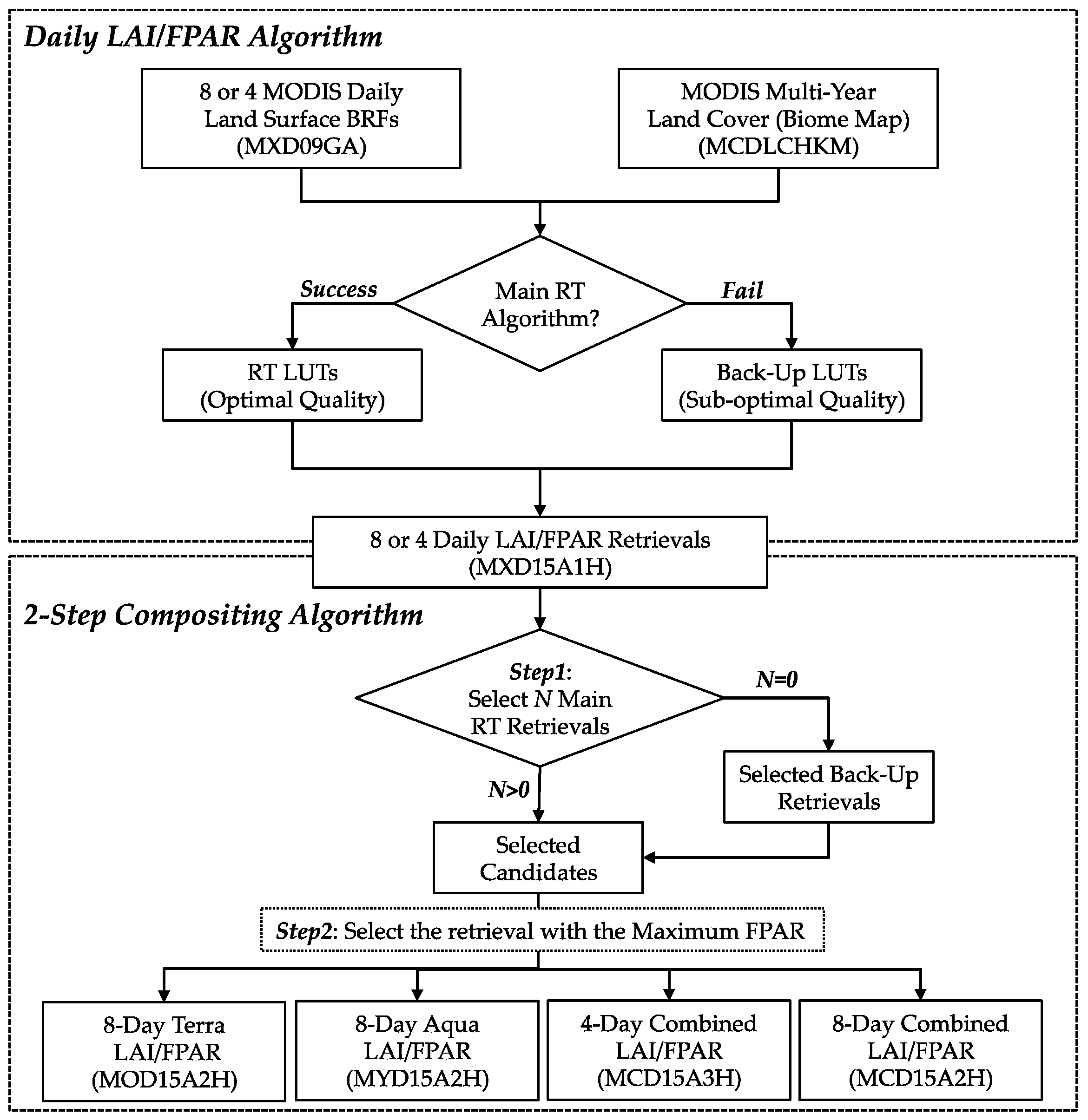
Figure 1 shows the flow of MODIS LAI/FPAR C6 production. The algorithm ingests MODIS daily red and near-infrared (NIR) BRFs and a biome map to generate daily LAI/FPAR retrievals without pre-quality-control on inputs. A temporal compositing approach is used to select the best retrievals and generate 8-day or 4-day products from daily retrievals. The compositing algorithm is a two-step scheme: (1) the retrievals are selected according to algorithm path: main algorithm retrievals have the highest priority, and if none are available, back-up algorithm retrievals are selected; (2) the LAI value is selected based on maximum FPAR value [
8]. Compositing reduces the impact of day-to-day artificial variations in surface reflectance that are due to cloud and residual atmospheric effects and it is effective in removing contaminated retrievals. As well as LAI/FPAR values, MODIS products store the corresponding quality control (QC) data layers and the users are advised to consult the quality flags when using these products [
7]. The key indicator of the quality of retrievals is the algorithm path, which distinguishes the following five categories: (1) main algorithm without saturation; (2) main algorithm with saturation; (3) back-up algorithm due to bad geometry; (4) back-up algorithm due to other problems; and (5) not produced. In addition to algorithm path, the QC layer provides information about presence of clouds, aerosols, and snow, inherited from input reflectance products.
2.4. Improvements of Collection 6
MODIS LAI/FPAR C6 uses the same science algorithm and LUTs as C5. However, this new version can still benefit from improved inputs as discussed below. As the only two inputs, the intermediate data at 1 km resolution of surface reflectances and biome map are replaced by their 500 m version, thus enabling the C6 LAI/FPAR products to have half-kilometer spatial resolution. The significance of this upgrade is two-fold. First, downstream land surface models can benefit from this finer resolution LAI/FPAR products. Second, the LAI/FPAR algorithm uses biome type classification to reduce unknown parameters and each pixel is assumed to belong to only one biome type with some pre-set structural and optical parameters. This assumption is more likely to be satisfied at finer resolutions because of the higher heterogeneity in coarse pixels [
21]. Moreover, the smaller pixel ground coverage can reduce the scale gap between remote sensing pixels and ground point measurements, which will reduce uncertainties and human labor during the process of products validation using ground measurements [
6,
22].
The new version of publicly available MODIS daily surface reflectances (MOD09GA C6) is used to replace the previous intermediate dataset (MODAGAGG) which was generated by aggregating four MOD09GA C5 pixels [
23]. This makes it possible for the community to test their own LAI/FPAR algorithms and compare with MODIS products. Improved aerosol retrieval and correction algorithm are employed in the generation of MOD09GA C6 dataset. Moreover, BRDF database is used to better constrain the thresholds used in the snow/cloud detection algorithm. MODIS land-cover product C5 (as input for LAI/FPAR C6) is also reported to be significantly improved through algorithm refinement and input data revise. Comparison of C5 land-cover with C4 (as input for LAI/FPAR C5) showed substantial differences. Cross-validation accuracy assessment indicates an overall accuracy of 75% in C5 land-cover product [
24]. In addition, C6 LAI/FPAR replaced the static land-cover input with new multi-year land-cover maps generated with three years of C5 land-cover data. Compared with the previous static land-cover, this new biome type source has a three-year temporal resolution and thus can capture the dynamic changes of biome types. According to previous experience [
1,
7], C6 LAI/FPAR products can benefit from the improved upstream reflectance and land-cover products [
25].
3. Consistency between C5 and C6 LAI/FPAR Products
Good consistency between different product versions creates confidence in LAI/FPAR data sets in both product producers and users, while poor consistency such as large differences diverts attention away from both of them. In this paper, we study the consistency between C5 and C6 along four fronts as discussed below. Note that, except for
Section 3.1 and
Section 3.4, we only focus on the retrievals from the main algorithm.
3.1. Global Distribution
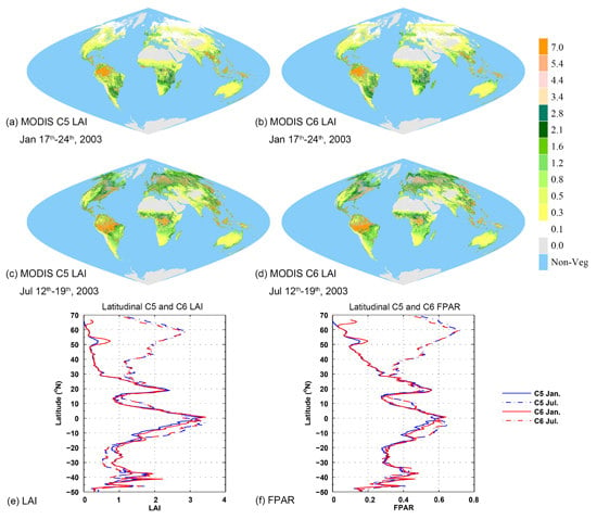
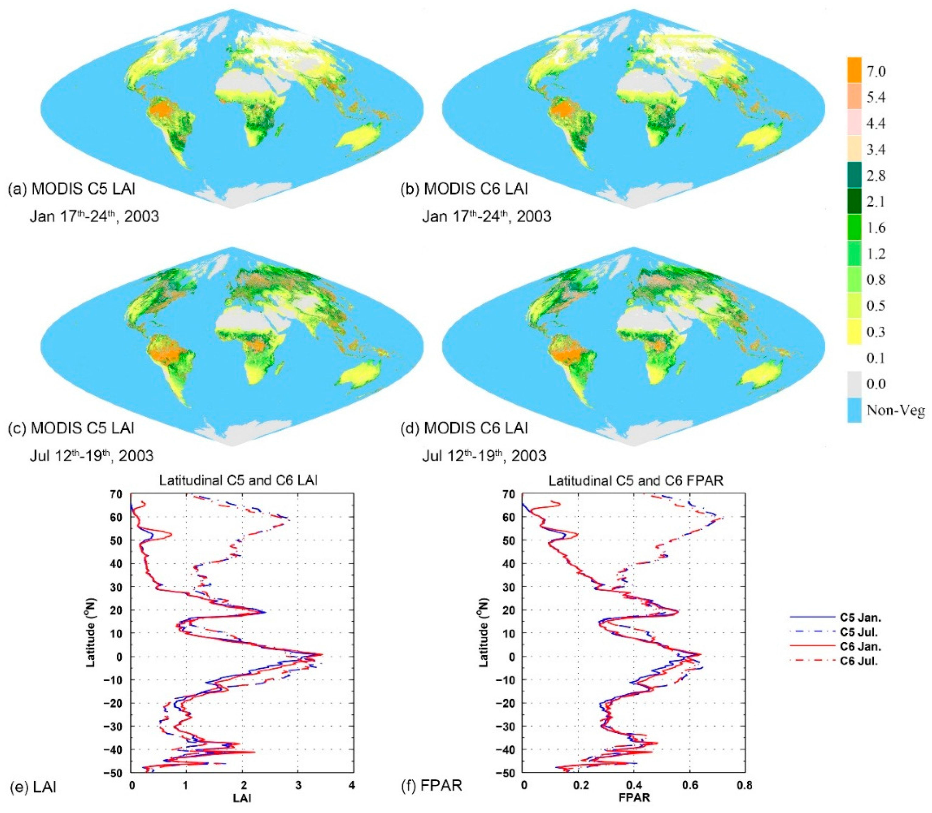
The spatial distribution of LAI and FPAR over the globe during two 8-day composite periods in January and July in the year 2003 are shown in
Figure 2a,d and
Figure S2. For both LAI and FPAR, there is no visually distinguishable difference between C5 and the new C6. The products from two collections exhibit similar spatial patterns. FPAR shows a similar distribution pattern to LAI, which can be explained by radiative transfer theory [
1]. The LAI patterns closely coincide with the biome type distribution (
Figure S1)—high LAI over forests and low LAI over herbaceous vegetation. As expected, tropical evergreen forests (e.g., amazon rain forests) have high LAI values (up to 7); somewhat less green are the middle latitude broadleaf forests (e.g., eastern United States). Except bare land and deserts, regions covered by grasses and shrubs generally have low LAI values. The globe looks greener in boreal summer time because of ample illumination conditions over the northern hemisphere, which has greater land surface.
Figure 2e,f compare the zonal mean LAI and FPAR values from C5 and C6 in January and July. For both LAI and FPAR, the profiles derived from C6 and C5 products match well at most latitude bands and show consistent latitudinal distribution of LAI and FPAR values. There are two obvious peaks in the tropics (23°N–23°S) which can be explained by the dense vegetation coverage in the three tropical rainforests (South America, Africa and Southeast Asia). As illumination is ample, there is no obvious seasonal difference in these latitude bands. In the higher latitudes, the northern hemisphere shows clear seasonal difference than the southern hemisphere. This is because the dominant biome types in the southern hemisphere are savannas, shrubs and grasses that have smaller seasonal variations than the forests that dominate the northern hemisphere [
26] (see
Figure S1). We also notice that C5 underestimates C6 in the bands 50°N–55°N and 63°N–70°N. This is caused by changes in input biome type and will be further discussed in
Section 4.1.
3.2. Spatial Coverage of Main Algorithm
As a key indicator of the quality of retrievals, the algorithm path of each pixel is stored in the LAI/FPAR products. By comparing the retrieval rate of different algorithm paths at global scale, we can evaluate the overall quality of the products from C5 and C6. The main algorithm outputs retrievals at high precision in the case of low LAI and at moderate precision when LAI is high and surface reflectance has low sensitivity to LAI. In the case of main algorithm failure, low-precision retrievals are obtained from the empirical back-up algorithm.
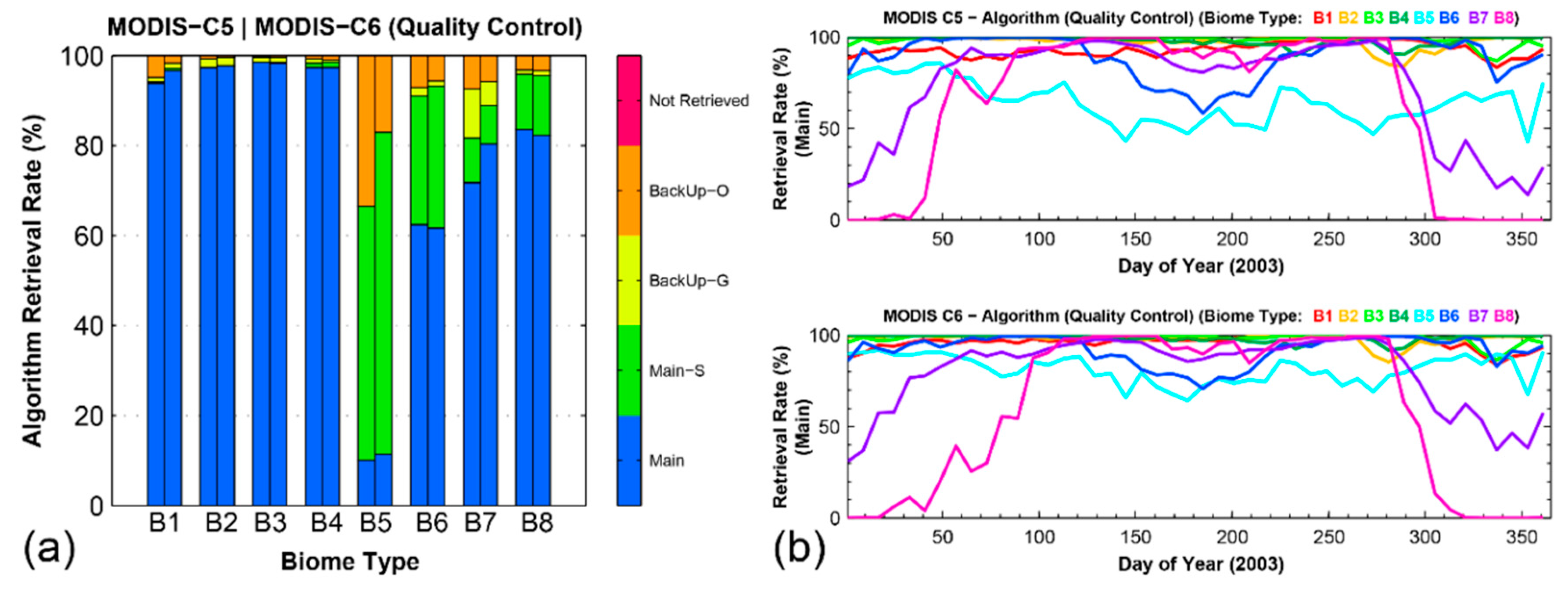
Figure 3a compares the biome-specific yearly and globally averaged retrieval rate of different algorithm paths. C6 and C5 show similar patterns for all biomes except biome 5 (evergreen broadleaf forests) and biome 7 (evergreen needleleaf forest). C6 shows 17% and 7% higher main algorithm retrieval rates than C5 for biomes 5 and 7, respectively. This improvement is due to an updated biome map, which will be discussed in
Section 4.1. As the main algorithm has better performance than the backup algorithm, the success rate of the main algorithm (Retrieval Index, RI) can be seen as a quality indicator. The RI of all biome types except biomes 5 and 7 is higher than 90%. Biomes 1 to 4 have the highest RI (more than 95%). The retrieval rate of main algorithm without saturation is lowest in the case of evergreen broadleaf forests because of reflectance saturation in dense canopies. This means the reflectances do not contain sufficient information to localize a LAI value. The other three forest types also show a large proportion of retrievals under saturation. Because evergreen needleleaf forests are located in the high latitude regions where the solar zenith angles are low in winter season, biome 7 shows obvious backup algorithm retrievals that are due to poor sun-sensor geometry. Nevertheless, C6 shows slightly higher RI than C5.
The seasonal variations of RI in C5 and C6 for all eight biomes in 2003 shown in
Figure 3b indicate that the annual cycles of C6 and C5 are quite consistent. As in
Figure 3a, the RI of biome 5 has been improved from C5 to C6. A strong seasonality is seen in needleleaf forests (biomes 7 and 8) with RI varying from about 90% during the boreal summer to less than 30% during the boreal winter. The RI of deciduous needleleaf forests can even be zero in the boreal winter season. The decrease of RI in the boreal winter results from unsuitable illumination conditions, extreme solar zenith angles, and snow or cloud contamination. The fact that almost all needleleaf forests appear only in the northern hemisphere makes the seasonal variation more obvious.
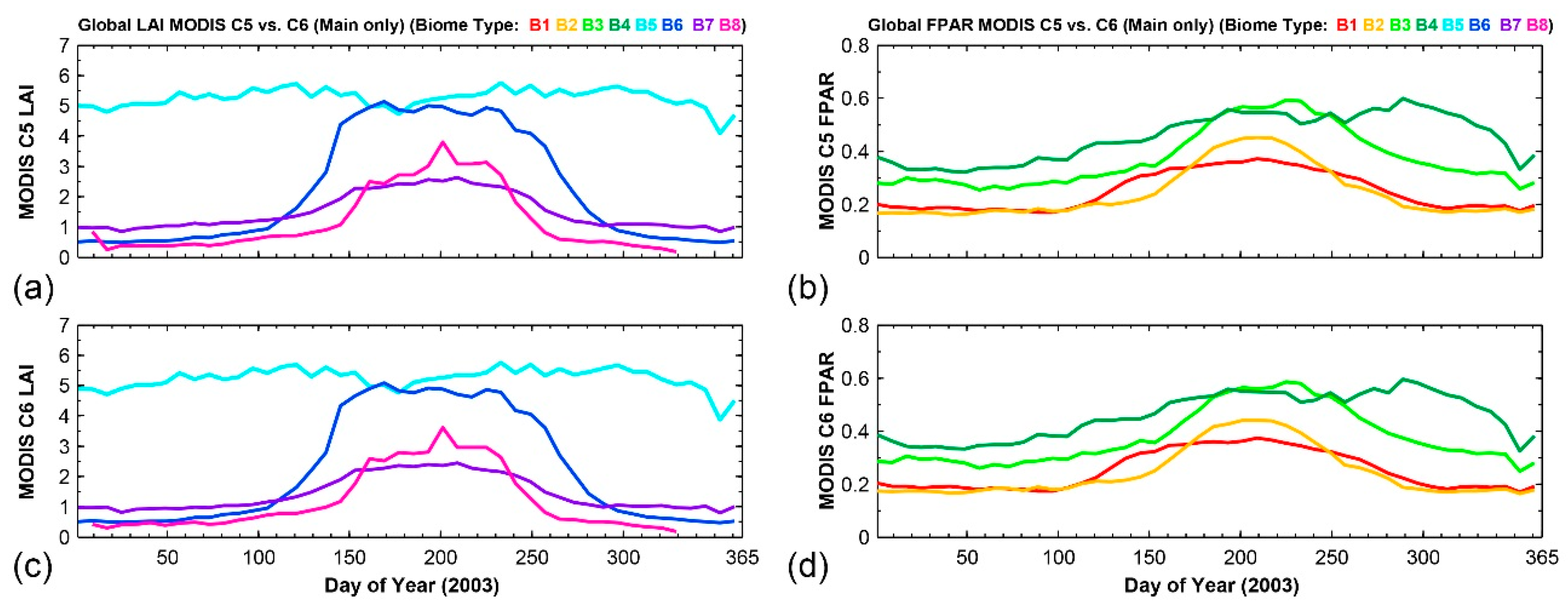
3.3. Seasonal LAI/FPAR Variations
Seasonal variations in C5 and C6 LAI/FPAR retrievals are shown in
Figure 4 and
Figure S3. These lines show globally averaged biome-specific LAI/FPAR values as a function of Julian day in 2003. This analysis only uses retrievals derived by the main algorithm. We note that C5 and C6 products show good consistency of LAI/FPAR seasonal variations. All biome types except for evergreen broadleaf forests and savannas show seasonality at different levels. The retrievals over deciduous forests demonstrate expected obvious seasonality in both LAI and FPAR. LAI of deciduous broadleaf forests (deciduous needleleaf forests) drops from around 5 (3) in boreal summer to around 0.5 (<0.5) in boreal winter. With ample illumination in tropics and subtropics, evergreen broadleaf forests have LAI values of about 5 through the year with negligible seasonal variations. By checking the seasonal variations of the algorithm path (see
Figure S4), we find that the missing part in case of deciduous needleleaf forests is due to unavailable retrievals from main algorithm because of bad sun-sensor geometry (solar zenith angle larger than 52.5° or view zenith angle larger than 67.5°). Seasonal variations of algorithm path can also explain these erratic artifacts in LAI/FPAR variations (e.g., the sudden drop at DOY 10 to 20 and the peak around DOY 200 for deciduous needleleaf forests in
Figure 4a).
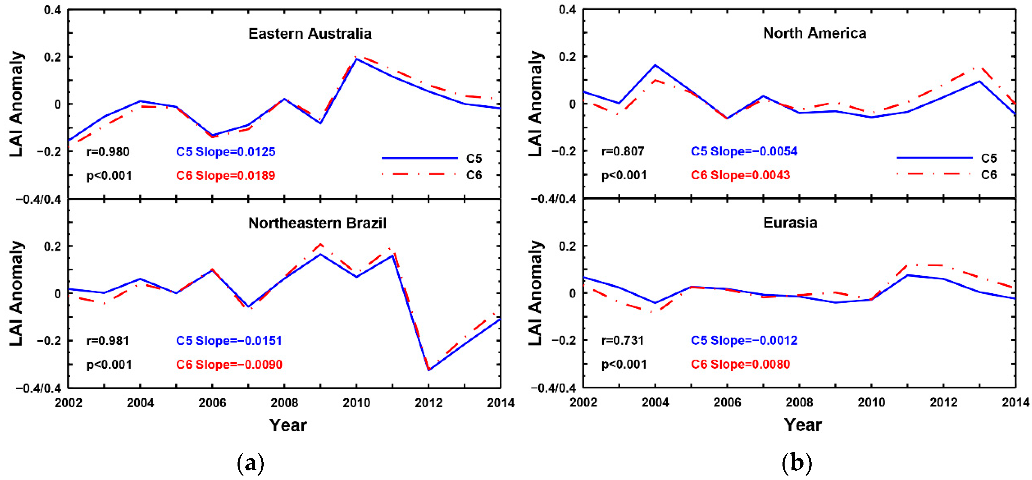
3.4. Inter-Annual LAI Anomalies
In this section, we check the consistency of 13 years (2002–2014) of LAI anomalies from C5 and C6. The importance of this work is two-fold. First, an LAI anomaly represents the difference between LAI values of a specific year and the multi-year mean LAI value, from which we can deduce potential annual variations in carbon, water and energy balances. Second, using independent geographic variables to explain the annual variation of LAI is a good way to validate the products indirectly.
The spatial and temporal averages of LAI anomalies from C5 and C6 during the period from 2002 to 2014 (2000 and 2001 were discarded because of missing data) are compared in
Figure 5. Panel (a) shows the anomaly of annual averaged LAI in two precipitation-limited regions (Eastern Australia and Northeastern Brazil). For both regions, C5 and C6 LAI anomalies match very well. The correlation coefficients between C5 and C6 in the two regions are 0.972 and 0.975, respectively. The LAI in Northeastern Brazil shows a large decrease in 2012, which can be explained by the severe drought in Northeast Brazil in that year [
27]. Panel (b) shows anomaly of growing season (May to September) averaged LAI in two temperature-limited regions (North America and Eurasia). Also for these two regions, C5 and C6 show similar LAI annual variations. We note that the slopes of C6 are slightly higher than C5 in all these plots. This is because the improved sensor calibration of C6 solved the Terra MODIS sensor degradation issue in C5 [
28]. A more detailed explanation for these LAI inter-annual variations will be presented in the second part of this two-paper series.
4. Benefits from Improved Input Data
From the above comparisons, we see there are no significant discrepancies between C5 and C6 products in terms of global distribution, seasonal variations, inter-annual LAI anomalies and spatial coverage of high quality retrievals. However, pixel-to-pixel comparison still shows differences between C5 and C6 at the regional scale. As C6 inherits the algorithm and LUTs from C5 directly, the improvements in input data and change of spatial resolution are the only two sources of LAI/FPAR differences between the two versions. Here we investigate and quantify the impact of input changes and the scale effect of the algorithm.
4.1. Benefits from Biome Map Improvement
As an important prior knowledge about the land surface, a biome map is utilized to reduce the number of unknowns in the inverse problem of LAI/FPAR estimation. In the operational algorithm, structurally and spectrally different parameterization in 3D RT is used for each biome type. Specification of biome type for each pixel is thus critically important to choose the correct RT dependent LUT for LAI/FPAR estimation. Errors in biome classification can therefore propagate into LAI/FPAR retrievals. Numerical experiments suggest that a mismatch in biome specific LUT will result in either a low RI and/or incorrect LAI/FPAR values [
1]. Conversely, increased biome accuracy will help to reduce uncertainty in LAI/FPAR products. As LAI/FPAR production requires prior knowledge of surface biome type, the biome input is generally based on an earlier version of land-cover product. This means C4 and C5 land-cover products have been used for C5 and C6 LAI/FPAR production, respectively. Biome input (based on C5 MODIS land-cover product) for C6 LAI/FPAR production is reported to be substantially improved relative to the biome input (based on C4 MODIS land-cover product) for C5 LAI/FPAR production in terms of accuracy, stability across years due to refinements in the land-cover classification algorithm and ancillary datasets used [
24].
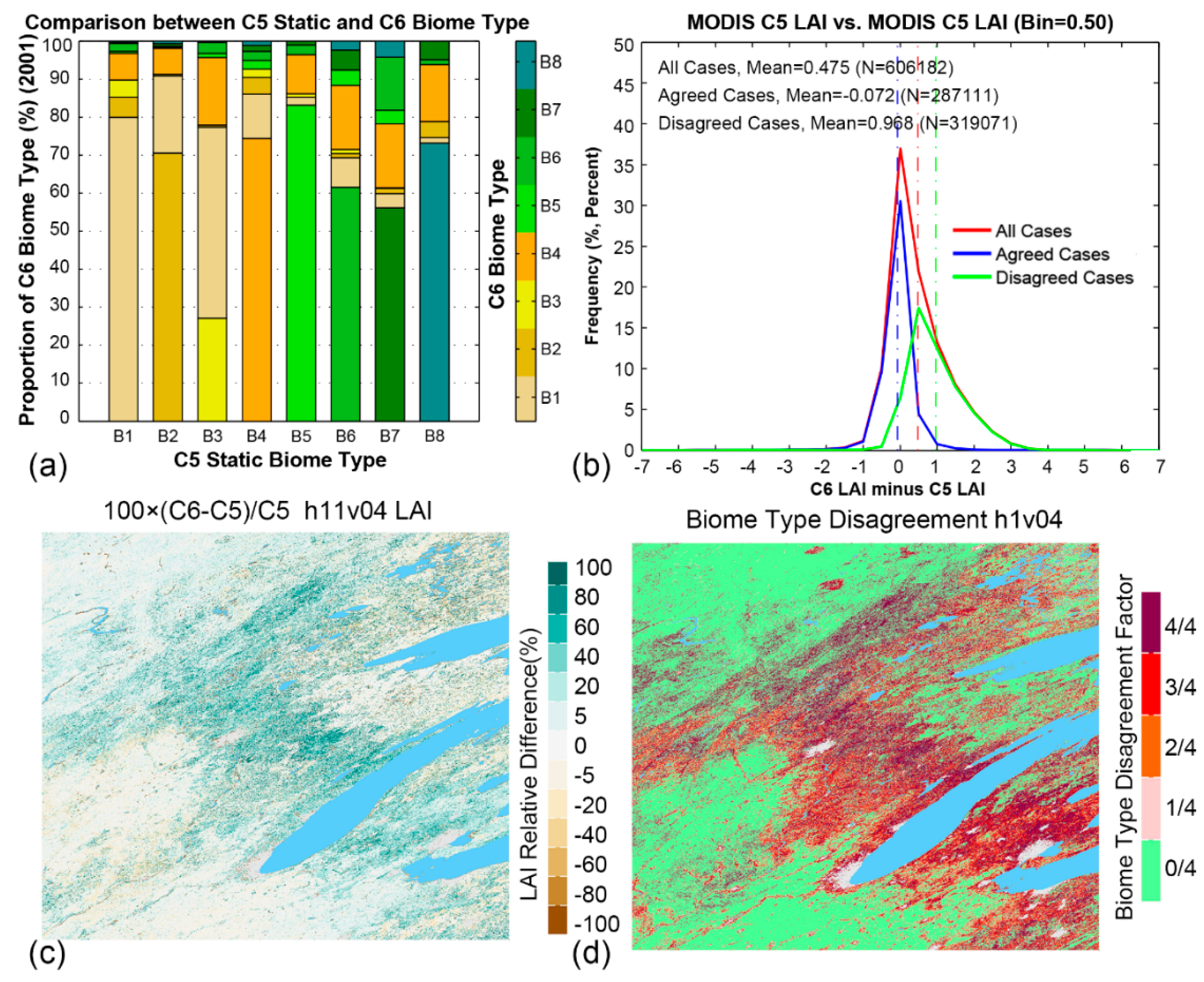
Figure 6a shows the proportion of pixels derived from each biome type in the C6 biome map for each class in the C5 biome type at the global scale during 2001 to 2003. Some biomes in C6, for example biomes 1, 2, 4, 5 and 8, are relatively consistent with C5 (more than 70% consistency). Around 30% of the pixels labeled as biome 6 and biome 7 in C5 change to other biome types in C6. Compared to other biomes, biome 3 has the largest proportion of differently classified biome cases. Around 50% of biome 3 pixels in C5 are classified into biome 1 in C6. We note that most of the differently classified pixels change to their neighboring biome types, which have similar canopy structural characteristics in RT realization. For instance, most of the “changed” pixels in biome 3 (broadleaf crops) are labeled as biome 1 (grass and cereal crop) in C6. This result agrees with [
24].
To quantify the impact of biome type change on LAI retrievals, we investigate the tile (1200 by 1200 km) h11v04 as an example as 53% of this region shows changes between C5 and C6. We divide all pixels into two categories, pixels with consistent and changed biome types, and compare the LAI differences. Histograms of the difference for these two categories and for all pixels are shown in
Figure 6b. The mean difference of all pixels with consistent biome type (about 27% of pixels) is −0.072, which is obviously smaller than that of all pixels with changing biome types (0.968). The mean difference of all pixels in this tile is 0.475. Such biased patterns are depicted in
Figure 6c,d. For further investigation, we define the biome type disagreement factor (BTDF) as the proportion of pixels with changing biome type. As four 500 m C6 pixels compose a 1 km C5 biome type, this factor can be 0, 1/4, 1/2, 3/4 or 1. It can be seen that when there is no biome type change, the relative difference in LAI will be within ±5%. This can be as high as ±100% in pixels with changing biome type. In particular, note that the directionality of observed difference is not uniform across cases of biome change.
The mean value and standard deviation of the difference and RMSE between C5 and C6 LAI are listed in
Table 1 (
Table S1 shows the same for FPAR). When the biome type disagreement factor is small (0/4 or 1/4), C6 retrievals underestimate C5 for most biome type cases. Interestingly, the discrepancy between C5 and C6 gets larger with increasing biome type disagreement factor. With the same biome input (BTDF = 0/4), the mean RMSE of LAI and FPAR are 0.29 and 0.091, respectively, but biome type disagreement worsened the consistency (LAI: 0.39, FPAR: 0.102). Overall C6 estimates global LAI and FPAR by C5-0.01 and C5-0.004, respectively.
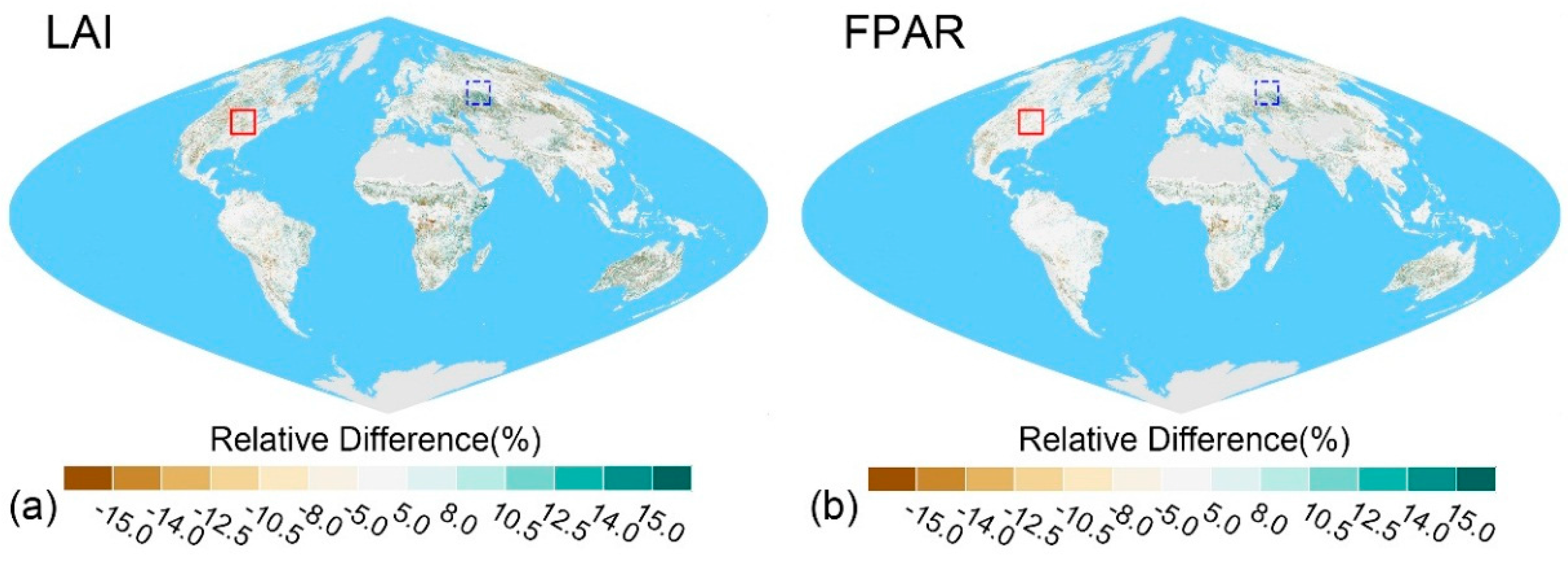
4.2. Benefits from Surface Reflectance Improvement
To elucidate the impact of changes in input surface reflectance, we only focus on pixels with consistent biome type (BTDF = 0). Between
Table 1 and
Table S1, we can see that C6 LAI and FPAR values of all biomes, except biomes 1 and 4 for LAI and biome 4 for FPAR, are smaller than C5.
Figure 7a,b shows the global distribution of relative difference (100 × (C6-C5)/C5) of LAI and FPAR. h11v04 (red box) and h22v03 (blue box) are two example tiles showing lower and higher C6 LAI estimation cases, respectively. As expected, both LAI and FPAR display similar spatial patterns. By only considering biome input consistent pixels, differences in LAI and FPAR between C5 and C6 vary within ±15%. Possible explanations for this discrepancy are two-fold: surface reflectance input changes and scale effect of the algorithm, further discussed below.
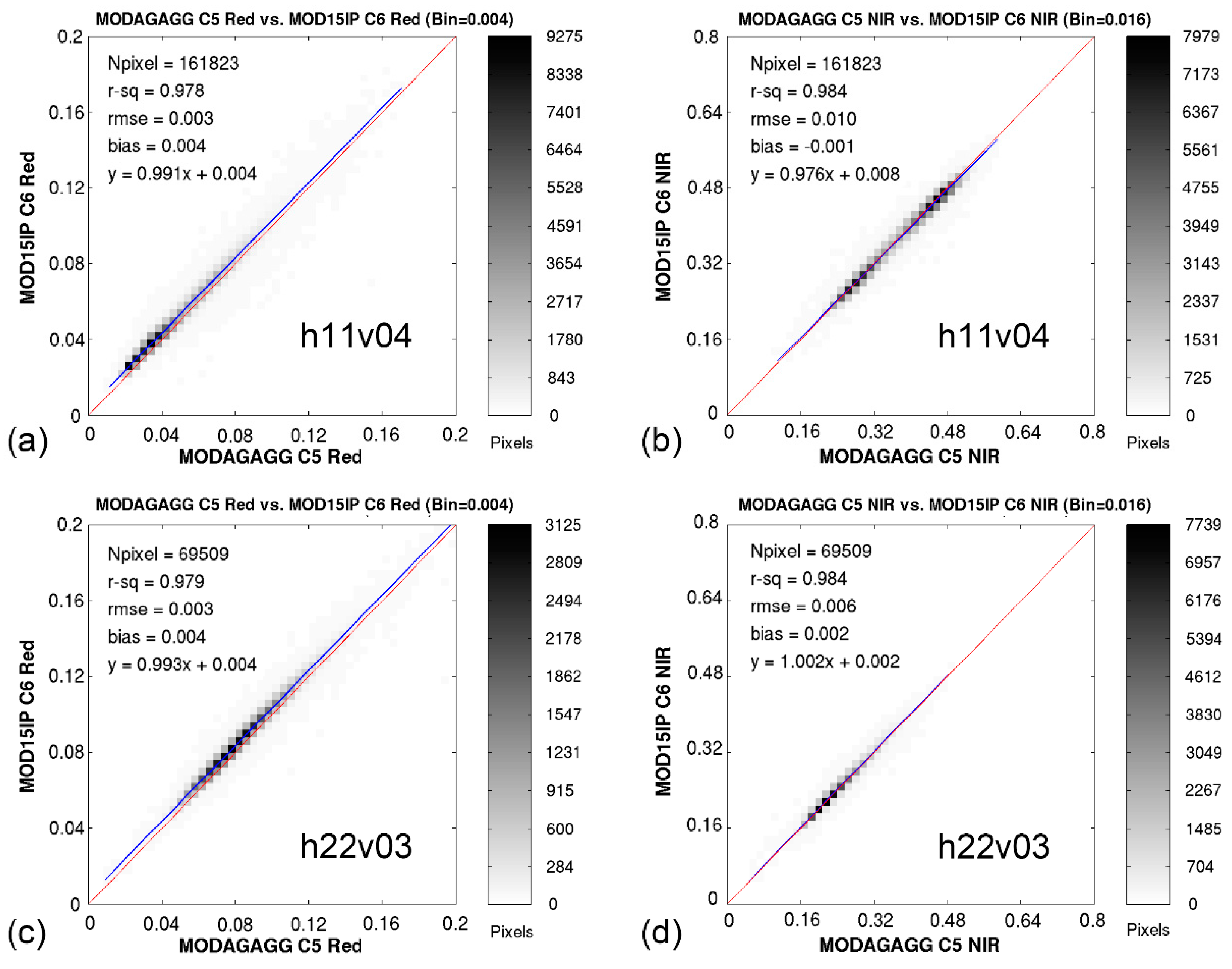
Comparisons of reflectance between C5 and C6 are shown in
Figure 8. Panels (a) and (b) are for tile h11v04 (
Figure 7) in which C6 underestimates C5. Panels (c) and (d) are for tile h22v03 (
Figure 7) in which C6 overestimates C5. In both tiles, NIR (near-infrared) band reflectance shows good consistency between the two versions. However, the red band reflectances in C6 are relatively higher than in C5, especially at the lower range of reflectances. As leaves in the canopy absorb more red photons, higher red reflectances will lead to lower LAI retrievals. These changes in reflectances resulted from refinements to the atmospheric correction algorithm. The overestimation in C6 over the tile h22v03 could be explained by the scale effects which are discussed below.
4.3. Impact of Scale Effect
With the development of quantitative remote sensing, scale effects, as a common phenomenon, have attracted more and more attention from the community. The term “scale” is widely used in many other fields as with as remote sensing and has different meanings in various disciplines [
29]. In this paper, scale effects refer to the discrepancy between two products derived from the same algorithm but at different spatial resolutions. As mentioned above, MODIS LAI/FPAR products improved the spatial resolution from 1 km to 500 m using the same retrieval algorithm, which raises two questions: (1) what is the behavior of the scale effect in LAI/FPAR product and algorithm and (2) is the difference caused by the scale effect negligible?
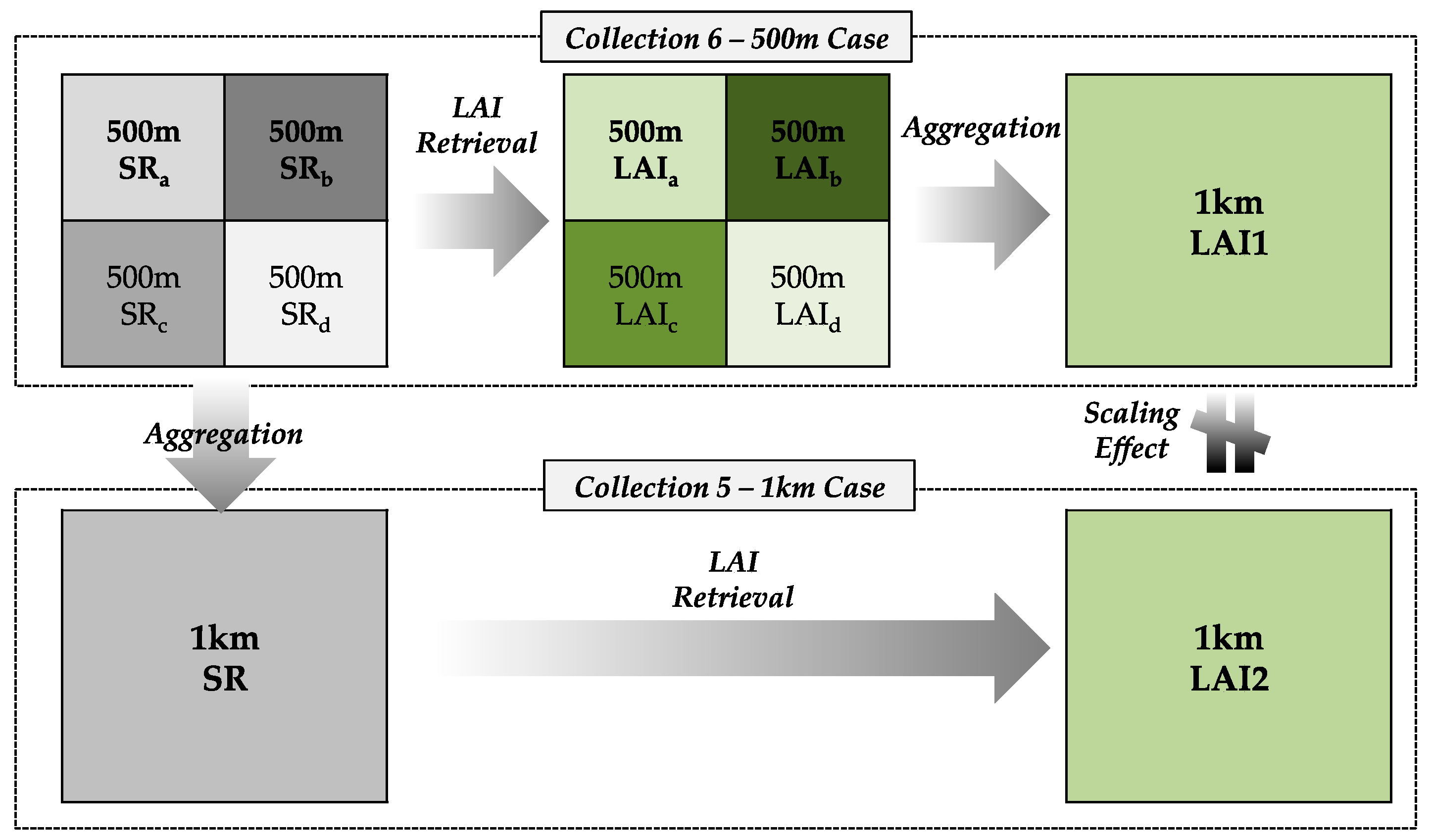
Figure 9 theoretically demonstrates the relationship between the two LAI products (C5 and C6). The discrepancy between LAI1 and LAI2 is caused by both heterogeneity of land surface and nonlinear characteristics of the retrieval models [
29]. On the one hand, landscape homogeneity cannot be assumed especially in the case of a coarser spatial resolution footprint. In other words, a MODIS pixel should be considered as a mosaic of different biome types. On the other hand, the radiative transfer-based algorithm is scale-dependent [
1]. This is because the pixels are likely to contain an increasing amount of radiative contribution from the background [
30]. Thus, the MODIS LAI/FPAR products are scale-dependent and the scale effect could be one of the causal factors introducing a certain level of discrepancy between C5 and C6.
To understand the discrepancy between C5 and C6 products due to scale effects, we conducted a simulation experiment using biome 6 (deciduous broadleaf forests) as an example. Note that the simulation results will not be similar across biome types due to biome-specific RT parameterizations. Only retrievals from the main RT based algorithm were analyzed. We simulated the heterogeneity in one 1 km (C5) pixel by adding 5% or 15% bias on NIR reflectance (red reflectance is fixed) for four 500 m (C6) pixels.
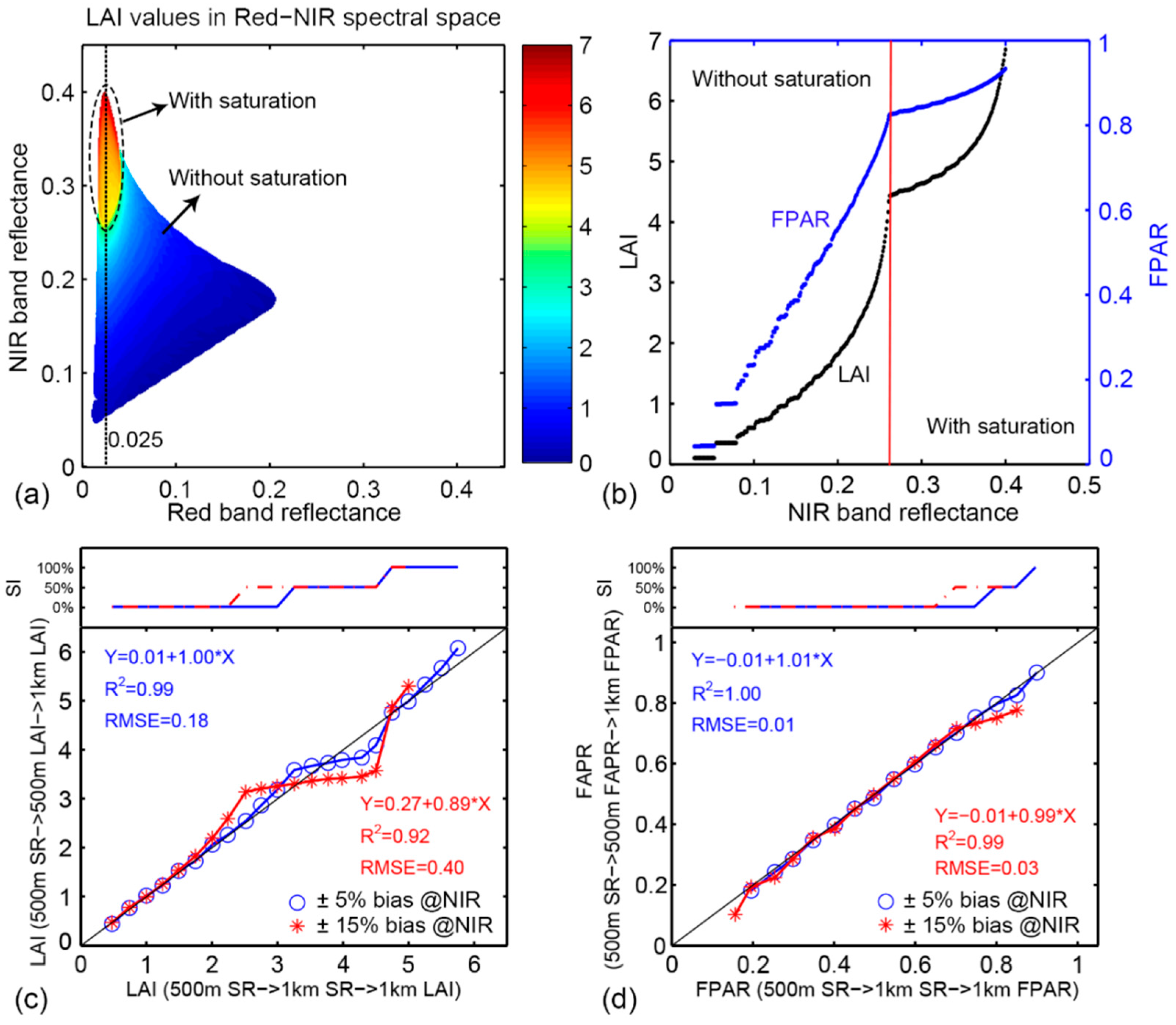
Figure 10 shows the results of this experiment. The LAI values for C5 were selected along the black line in the red-NIR spectral space depicted in
Figure 10a. It is clear that the relationship between LAI and reflectance is nonlinear. Moreover, there is a clear division between the saturated and unsaturated parts. This is more obvious in
Figure 10b where both LAI and FPAR show an inflection point when saturation appears. Irrespective of saturation, the relationship between LAI and NIR reflectance is roughly a concave function. In this relationship, if reflectance SR2 is the mean value of SR1 and SR3, the LAI (SR2) is smaller than the mean value of LAI (SR1) and LAI (SR3). Before saturation, the relationship between FPAR and NIR reflectance is almost linear. When saturation appears, the relationship changes to a concave function as well. The short parallel lines at small LAI and FPAR indicate that LAI or FPAR does not vary with NIR reflectance. This is because of sparse distribution of retrievals in the LUT at low LAI values [
31].
The discrepancy in LAI and FPAR due to scale effects is demonstrated in
Figure 10c,d. The x-axis and y-axis can be seen as C5 products and C6 products, respectively. The four retrievals of C6 pixels can be partially and completely derived from unsaturated or saturated algorithmic conditions because of the bias in NIR reflectance. We define the Saturation Index (SI) as the proportion of unsaturated pixels. When SI equals 0% (all retrievals from the unsaturated part), there is no obvious difference between C5 and C6 LAI values at a low range of LAI values. However, C6 LAI tends to be higher than C5 with an increase in LAI. When SI is about 50% (two retrievals from unsaturated and the other two from saturated part), C6 LAI tends to be smaller than C5. When SI equals 100%, C6 LAI increases again. These changes can be explained by the relationship between LAI and NIR reflectance shown in
Figure 10b. As expected, a 15% bias causes a larger scale effect than a 5% bias (RMSE 0.4
vs. 0.18). Compared to LAI, FPAR shows less and even negligible scale effects with RMSE 0.01 and 0.03 for 5% and 15% bias. This is because the FPAR-reflectance relationship is almost linear, especially prior to saturation conditions. Because of the regional convex relationship when saturation starts to appear, C6 can be lower than C5.
5. Conclusions
This paper presents version consistency and improvements in the latest MODIS LAI/FPAR C6 product. Compared to previous C5, the most important change in C6 is that the products are being produced at 500 m spatial resolution instead of 1 km. In addition, as discussed here, C6 benefited from improved surface reflectances and biome type inputs. The refined C6 atmospheric correction algorithm generates relatively higher red band reflectances, which results in lower LAI/FPAR values. The new multi-year land-cover product provides biome type input to the algorithm with better accuracy. The differences caused by scale effects are found to be negligible for FPAR and in cases where LAI is low. Scale effects can explain some of the discrepancy between 1 km C5 and 500 m C6 products, especially for cases of high LAI values. In view of these changes in inputs and spatial resolution, a consistency check of C6 products with C5 was performed in terms of global distributions, spatial coverage of high quality retrievals, seasonal variations and inter-annual LAI anomalies. From these analyses, we found no significant discrepancies between C5 and C6 LAI/FPAR products. The proportion of main radiative transfer algorithm retrievals in C6 increases slightly in most biome types, notably including 17% improvement in evergreen broadleaf forests. With the same biome input, the mean RMSEs of LAI and FPAR are 0.29 and 0.091, respectively, but biome type disagreement worsens the consistency (LAI: 0.39, FPAR: 0.102). Overall C6 estimates global LAI and FPAR by C5-0.01 and C5-0.004. Moreover, C5 and C6 shows consistent inter-annual LAI anomalies over two temperature-limited regions and two precipitation-limited regions. These results produce confidence in the new C6 products. Further evaluation of MODIS LAI/FPAR C6 products through validation using field measurements and inter-comparison with other exiting products will be presented in the second part of this series.
Supplementary Materials
The following are available online at
www.mdpi.com/2072-4292/8/5/359, Figure S1: Three-year global 500 m eight-biome map used for MODIS LAI/FPAR C6 products from 2001 to 2003; Figure S2: Color-coded maps of MODIS C5 and C6 FPAR for January (17th–24th January) and July (12th–19th July) of 2003; Figure S3: Seasonal variations of globally averaged MODIS LAI and FPAR from C5 and C6 in 2003; Figure S4: Seasonal variations of algorithm path of C5 and C6 in 2003; Table S1: Biome type specific differences between C5 and C6 FPAR for global scale in 2003.
Acknowledgments
Help from MODIS & VIIRS Science team members is gratefully acknowledged. This work is supported by the MODIS program of NASA and partially funded by the National Basic Research Program of China (Grant No. 2013CB733402), the key program of NSFC (Grant No. 41331171) and Chinese Scholarship Council.
Author Contributions
Kai Yan, Yuri Knyazikhin, Ramakrishna R. Nemani and Ranga B. Myneni conceived and designed the experiments; Taejin Park and Kai Yan performed the experiments; Chi Chen, Taejin Park and Bin Yang analyzed the data; Zhao Liu and Guangjian Yan contributed to
Section 3.4 and
Section 4.3, respectively. All authors contributed to the writing of the paper.
Conflicts of Interest
The authors declare no conflict of interest.
Abbreviations
The following abbreviations are used in this manuscript:
| MODIS | Moderate Resolution Imaging Spectroradiometer |
| LAI | Leaf Area Index |
| FPAR | Fraction of Photosynthetically Active Radiation |
| C3 | Collection 3 |
| C4 | Collection 4 |
| C5 | Collection 5 |
| C6 | Collection 6 |
| RT | Radiative Transfer |
| LUT | Look-Up-Table |
| BRF | Bi-directional Reflectance Factors |
| NDVI | Normalized Difference Vegetation Index |
| QC | Quality Control |
| BTDF | Biome Type Disagreement Factor |
| RI | Retrieval Index |
| SI | Saturation Index |
References
- Myneni, R.B.; Smith, G.R.; Lotsch, A.; Friedl, M.; Morisette, J.T.; Votava, P.; Running, S.W.; Hoffman, S.; Knyazikhin, Y.; Privette, J.L.; et al. Global products of vegetation leaf area and fraction absorbed PAR from year one of MODIS data. Remote Sens. Environ. 2002, 83, 214–231. [Google Scholar] [CrossRef]
- Sellers, P.J.; Dickinson, R.E.; Randall, D.A.; Betts, A.K.; Hall, F.G.; Berry, J.A.; Collatz, G.J.; Denning, A.S.; Mooney, H.A.; Nobre, C.A. Modeling the exchanges of energy, water, and carbon between continents and the atmosphere. Science 1997, 275, 502–509. [Google Scholar] [CrossRef] [PubMed]
- Zhu, Z.; Bi, J.; Pan, Y.; Ganguly, S.; Anav, A.; Xu, L.; Samanta, A.; Piao, S.; Nemani, R.; Myneni, R. Global data sets of vegetation leaf area index (LAI)3g and Fraction of Photosynthetically Active Radiation (FPAR)3g derived from Global Inventory Modeling and Mapping Studies (GIMMS) Normalized Difference Vegetation Index (NDVI3g) for the Period 1981 to 2011. Remote Sens. 2013, 5, 927–948. [Google Scholar]
- Knyazikhin, Y.; Martonchik, J.V.; Myneni, R.B.; Diner, D.J.; Running, S.W. Synergistic algorithm for estimating vegetation canopy leaf area index and fraction of absorbed photosynthetically active radiation from MODIS and MISR data. J. Geophys. Res. Atmos. 1998, 103, 32257–32275. [Google Scholar] [CrossRef]
- Knyazikhin, Y.; Glassy, J.; Privette, J.L.; Tian, Y.; Lotsch, A.; Zhang, Y.; Wang, Y.; Morisette, J.T.; Votava, P.; Myneni, R.B. MODIS Leaf Area Index (LAI) and Fraction of Photosynthetically Active Radiation Absorbed by Vegetation (FPAR) Product (MOD15) Algorithm Theoretical Basis Document; Theoretical Basis Document; NASA Goddard Space Flight Center: Greenbelt, MD, USA, 1999; pp. 1–170. [Google Scholar]
- Yang, W.; Tan, B.; Huang, D.; Rautiainen, M.; Shabanov, N.V.; Wang, Y.; Privette, J.L.; Huemmrich, K.F.; Fensholt, R.; Sandholt, I.; et al. MODIS leaf area index products: From validation to algorithm improvement. IEEE Trans. Geosci. Remote Sens. 2006, 44, 1885–1898. [Google Scholar] [CrossRef]
- Yang, W.; Huang, D.; Tan, B.; Stroeve, J.C.; Shabanov, N.V.; Knyazikhin, Y.; Nemani, R.R.; Myneni, R.B. Analysis of leaf area index and fraction of PAR absorbed by vegetation products from the terra MODIS sensor: 2000–2005. IEEE Trans. Geosci. Remote Sens. 2006, 44, 1829–1842. [Google Scholar] [CrossRef]
- Yang, W.; Shabanov, N.V.; Huang, D.; Wang, W.; Dickinson, R.E.; Nemani, R.R.; Knyazikhin, Y.; Myneni, R.B. Analysis of leaf area index products from combination of MODIS Terra and Aqua data. Remote Sens. Environ. 2006, 104, 297–312. [Google Scholar] [CrossRef]
- Shabanov, N.V.; Knyazikhin, Y.; Baret, F.; Myneni, R.B. Stochastic Modeling of Radiation Regime in Discontinuous Vegetation Canopies. Remote Sens. Environ. 2000, 74, 125–144. [Google Scholar] [CrossRef]
- Buermann, W. Analysis of a multiyear global vegetation leaf area index data set. J. Geophys. Res. 2002, 107, D22. [Google Scholar] [CrossRef]
- Ganguly, S.; Samanta, A.; Schull, M.A.; Shabanov, N.V.; Milesi, C.; Nemani, R.R.; Knyazikhin, Y.; Myneni, R.B. Generating vegetation leaf area index Earth system data record from multiple sensors. Part 2: Implementation, analysis and validation. Remote Sens. Environ. 2008, 112, 4318–4332. [Google Scholar] [CrossRef]
- Fang, H.; Jiang, C.; Li, W.; Wei, S.; Baret, F.; Chen, J.M.; Garcia-Haro, J.; Liang, S.; Liu, R.; Myneni, R.B.; et al. Characterization and intercomparison of global moderate resolution leaf area index (LAI) products: Analysis of climatologies and theoretical uncertainties. J. Geophys. Res. Biogeosci. 2013, 118, 529–548. [Google Scholar] [CrossRef]
- Majasalmi, T.; Rautiainen, M.; Stenberg, P.; Manninen, T. Validation of MODIS and GEOV1 fPAR Products in a Boreal Forest Site in Finland. Remote Sens. 2015, 7, 1359–1379. [Google Scholar] [CrossRef]
- Garrigues, S.; Lacaze, R.; Baret, F.; Morisette, J.T.; Weiss, M.; Nickeson, J.E.; Fernandes, R.; Plummer, S.; Shabanov, N.V.; Myneni, R.B.; et al. Validation and intercomparison of global Leaf Area Index products derived from remote sensing data. J. Geophys. Res. 2008, 113. [Google Scholar] [CrossRef]
- Ross, J. The Radiation Regime and Architecture of Plants Stands; Springer Science & Business Media: Medford, MA, USA, 1981. [Google Scholar]
- Myneni, R.B.; Ross, J. Photon-Vegetation Interactions: Applications in Optical Remote Sensing and Plant Ecology; Springer Science & Business Media: Medford, MA, USA, 1991. [Google Scholar]
- Huang, D.; Knyazikhin, Y.; Dickinson, R.E.; Rautiainen, M.; Stenberg, P.; Disney, M.; Lewis, P.; Cescatti, A.; Tian, Y.; Verhoef, W.; et al. Canopy spectral invariants for remote sensing and model applications. Remote Sens. Environ. 2007, 106, 106–122. [Google Scholar] [CrossRef]
- Myneni, R.B.; Williams, D.L. On the relationship between FAPAR and NDVI. Remote Sens. Environ. 1994, 49, 200–211. [Google Scholar] [CrossRef]
- Wang, Y.; Tian, Y.; Zhang, Y.; El-Saleous, N.; Knyazikhin, Y.; Vermote, E.; Myneni, R.B. Investigation of product accuracy as a function of input and model uncertainties: Case study with SeaWiFS and MODIS LAI/FPAR algorithm. Remote Sens. Environ. 2001, 78, 299–313. [Google Scholar] [CrossRef]
- Myneni, R.B.; Ramakrishna, R.; Nemani, R.; Running, S.W. Estimation of global leaf area index and absorbed par using radiative transfer models. IEEE Trans. Geosci. Remote Sens. 1997, 35, 1380–1393. [Google Scholar] [CrossRef]
- Fang, H.; Li, W.; Myneni, R.B. The impact of potential land cover misclassification on MODIS leaf area index (LAI) estimation: A statistical perspective. Remote Sens. 2013, 5, 830–844. [Google Scholar] [CrossRef]
- Garrigues, S.; Shabanov, N.V.; Swanson, K.; Morisette, J.T.; Baret, F.; Myneni, R.B. Intercomparison and sensitivity analysis of Leaf Area Index retrievals from LAI-2000, AccuPAR, and digital hemispherical photography over croplands. Agric. Forest Meteorol. 2008, 148, 1193–1209. [Google Scholar] [CrossRef]
- Vermote, E.F.; Vermeulen, A. Atmospheric Correction Algorithm: Spectral Reflectances (MOD09). Algorithm Theoretical Background Document. Available online: http://dratmos.geog.umd.edu/files/pdf/atbd_mod09.pdf (accessed on 7 March 2016).
- Friedl, M.A.; Sulla-Menashe, D.; Tan, B.; Schneider, A.; Ramankutty, N.; Sibley, A.; Huang, X. MODIS Collection 5 global land cover: Algorithm refinements and characterization of new datasets. Remote Sens. Environ. 2010, 114, 168–182. [Google Scholar] [CrossRef]
- Wolfe, R.E.; Devadiga, S.; Masuoka, E.J.; Running, S.W.; Vermote, E.; Giglio, L.; Wan, Z.; Riggs, G.A.; Schaaf, C.; Myneni, R.B.; et al. Improvements to the MODIS Land Products in Collection Version 6. Available online: http://adsabs.harvard.edu/abs/2013AGUFM.B41D0430W (accessed on 7 March 2016).
- Masson, V.; Champeaux, J.; Chauvin, F.; Meriguet, C.; Lacaze, R. A global database of land surface parameters at 1-km resolution in meteorological and climate models. J. Climat. 2003, 16, 1261–1282. [Google Scholar] [CrossRef]
- Marengo, J.A.; Alves, L.M.; Soares, W.R.; Rodriguez, D.A.; Camargo, H.; Riveros, M.P.; Pabló, A.D. Two contrasting severe seasonal extremes in tropical South America in 2012: Flood in Amazonia and drought in northeast Brazil. J. Climat. 2013, 26, 9137–9154. [Google Scholar] [CrossRef]
- Wang, D.; Morton, D.; Masek, J.; Wu, A.; Nagol, J.; Xiong, X.; Levy, R.; Vermote, E.; Wolfe, R. Impact of sensor degradation on the MODIS NDVI time series. Remote Sens. Environ. 2012, 119, 55–61. [Google Scholar] [CrossRef]
- Wu, H.; Li, Z. Scale Issues in Remote Sensing: A Review on Analysis, Processing and Modeling. Sensors 2009, 9, 1768–1793. [Google Scholar] [CrossRef] [PubMed]
- Tian, Y.; Wang, Y.; Zhang, Y.; Knyazikhin, Y.; Bogaert, J.; Myneni, R.B. Radiative transfer based scaling of LAI retrievals from reflectance data of different resolutions. Remote Sens. Environ. 2003, 84, 143–159. [Google Scholar] [CrossRef]
- Ganguly, S.; Schull, M.A.; Samanta, A.; Shabanov, N.V.; Milesi, C.; Nemani, R.R.; Knyazikhin, Y.; Myneni, R.B. Generating vegetation leaf area index earth system data record from multiple sensors. Part 1: Theory. Remote Sens. Environ. 2008, 112, 4333–4343. [Google Scholar] [CrossRef]
© 2016 by the authors; licensee MDPI, Basel, Switzerland. This article is an open access article distributed under the terms and conditions of the Creative Commons Attribution (CC-BY) license (http://creativecommons.org/licenses/by/4.0/).


 ,
, 


