Soil and Plant Nutrient Analysis with a Portable XRF Probe Using a Single Calibration

Abstract

A portable X-ray fluorescence probe (pXRF) is a tool that is used to measure many elements quickly and efficiently in various samples, without any pretreatment. However, each type of sample generally requires different calibrations to be accurate. To overcome this, our work evaluated the efficacy of determining several elements in forage plant samples using the ‘Soil Nutrient and Metal’ calibration in a commercially available pXRF probe, envisioning that a single calibration can be used to measure samples of different matrixes. For this, the net intensity of the pXRF probe was determined in place of the concentration values that are obtained directly from measurements. Elemental concentrations (P, K, Ca, Mg, S, Cu, Fe, Zn, and Mn) from forage plant samples, collected across Oklahoma, US, were assessed in a representative number of ‘modeling’ and ‘validation’ (independent dataset) samples. Linear regression (LR) associated with the d-index, polynomial regression (PR), and power regression (PwR) were tested for predictions, producing many statistical parameters associated with the models that were used for comparison goals. The pXRF elemental data provided highly reliable predictions of K, S, Zn, and Mn regardless of the regression model. Although all models can be reliable in prediction of Ca and Fe concentrations, the PwR provided better root mean square error (RMSE) values. The predictions of Mg concentrations were less reliable, although highly significant; however, the P and Cu predictions were not acceptable. Our work successfully showed that, once established, a single calibration curve that covers a wide range of concentrations of several elements in soils and plant tissues enables both soil and plant samples to be analyzed. This suggests that manufacturers can develop a new calibration model for a commercially available pXRF probe that covers a wide variety of heterogeneous samples.

1. Introduction

Research on the application of portable X-ray fluorescence probes (pXRF) for agricultural purposes has been very limited, and research regarding their use for plant analysis was nearly nonexistent [1]. Some works [1,2,3,4] have assessed pXRF probe use in determining plant nutrient concentrations, aiming to eliminate the wet chemistry sample preparations that are usually involved during acid digestion [5]. Although some inconsistent findings were reported, the use of pXRF probes on processed plant samples is commonly encouraged to eliminate both the acid digestion step and quantification by an inductively coupled plasma spectroscopy (ICP), since the nutrients concentration of plant tissues can be assessed in a matter of seconds with a pXRF probe. However, most of the calibration methods designed for commercially available pXRF probes are dedicated to soil and mineral samples [6], which makes it necessary to develop another calibration curve that is externally purchased, if the determination of elemental concentration in plant tissues is desired. Therefore, it is important to develop a single calibration curve with multiple purposes, with potential use for heterogeneous samples such as soils and plants. This would gradatively eliminate the costly use of time and resources that is involved in the standard method (wet chemical analysis via acid digestion and quantitative determination via ICP). Our work will be a pioneer in inspiring such a development, since a single calibration curve—originally designed for elemental analyses in soil samples—will be used to determine nutrient concentrations in forage plant tissues.

Foliar diagnosis has been used for a long time to evaluate plant nutritional status [4]. This evaluation is related to fertilizer application responses and access to the mineral composition of forage plant tissues for major ruminant livestock feeds [3]. Since these evaluations are presently a subject matter for study [4], it is important to make accessible the use of instruments that quickly determine the elemental composition. In this context, analysis by pXRF probes can be a superior alternative to wet chemistry in terms of both cost and time effectiveness [7], as well as in the analysis of samples that are not chemically pretreated or are totally non-destructive. Overall, the accurate determination of elemental composition depends on proper sample preparation and placement, instrumental setup of the pXRF probe, the energy level of the element, scanning time, particle size, and the moisture content of the sample [2]. Additionally, penetration and escape depths potentially influence pXRF analyses [3]. The former refers to the depth to which the primary X-ray penetrates the sample; thus, it depends on the sample matrix and the primary X-ray energy. The latter also depends on the sample matrix; however, the emerging fluorescent X-ray energy also becomes relevant. Thus, most of the works referred to previously have made use of software that determine the elemental concentration in plant tissues under their net intensity measurements—even under the specific calibration curves acquired for elemental concentration in plants—and correlates them with actual values from standard methods [1,3]. In this framework, we aimed to use the same technique to determine plant nutrient concentrations from a calibration method that was originally developed for soil analysis, since the range of elemental concentrations of forage plant samples used in our study is within the range of the calibration curve acquired by the pXRF probe. Moreover, the sample processing of forage plants is identical to that of soil, in terms of drying and particle size after grinding.

This study sought to evaluate the efficacy of using a calibration of a pXRF probe that was designed for soils (previously established and validated in the work of Zhang et al. [8]) to quantitatively predict nutrient (P, K, Ca, Mg, S, Cu, Fe, Zn, and Mn) concentrations in plant samples from Oklahoma (OK), US. Specifically, the objectives of the study were to: (1) assess the relationship between pXRF net intensity data and elemental concentration from a standard method, and (2) to establish predictive models that can accurately calculate the concentrations of P, K, Ca, Mg, S, Cu, Fe, Zn, and Mn from pXRF data, by identifying the best possible regression model. It was hypothesized that pXRF probes may be able to accurately predict nutrient contents in forage plant samples, using a single calibration method that was previously developed for soil analyses, since plant elemental concentrations fall within the range of the current calibration curve.

2. Materials and Methods

2.1. Forage Plant Samples Collection and Preparation

Forty plant samples were collected across Oklahoma, US, from field trials belonging to the Oklahoma State University (OSU) (Supplementary Figure S1). Most of the samples were comprised of cool- and warm-season forages such as annual ryegrass, wheat pasture, bermudagrass, and switchgrass. The harvested aboveground biomass (plant shoots) was washed with deionized water and oven-dried to a constant weight at 105 °C. Dried plant materials were ground to ≤2 mm particle size, using a mechanical grinder for further analyses by both wet chemistry and pXRF probe. The ≤2 mm particle size was chosen to simulate the same physical conditions of processed soil samples that can be measured by a pXRF probe, and because of the results of Sapkota et al. [3], who indicated that the heterogeneous nature of the forage plant sample did not affect the quality of results when samples are ground to ≤2 mm sizes. Moreover, after testing particle sizes of ≤1 mm and ≤0.25 mm, we found out that increasing the fineness or specific surface area did not affect the quality of measurements, and changes were either not significant or were negligible among samples (data not shown). Hence, the ≤2 mm particle size was chosen for analysis, since it is easier and faster to obtain in practice.

2.2. Wet Chemical Analysis (Standard Method)

Dried and ground plant materials were analyzed for mineral composition using nitric acid digestion, in which 0.5 g of each sample was predigested for 1 h with 10 mL of trace metal grade HNO₃ in the HotBlock™ Environmental Express block digester. Then, the digests were heated to 115 °C for 2 h and diluted with deionized water to 50 mL [9]. The digested samples were determined for P, K, Ca, Mg, S, Cu, Fe, Zn, and Mn by an inductively coupled plasma atomic emission spectroscopy (ICP-AES).

2.3. pXRF Probe Assays and Analysis

The pXRF measurements were performed using a TRACER 5i portable/handheld XRF spectrometer (Bruker, Kennewick, WA, USA). More details on the pXRF instrument can be found in Zhang et al. [8]. All analyses were performed using the ‘Soil Nutrient and Metal’ calibration provided by the manufacturer. Triplicate readings were taken at 50 kV, 39 µA, with a Duplex 2205 sample over the examination window, and rounded up to the nearest 5 µRem/hr value [8]. Samples were analyzed for 60 s using 2 phase scans for 30 s each phase. Recent results indicated that forage plant samples can be analyzed with as little as 60 s without losing accuracy [3]. Additionally, the 60 s time for elemental concentration determination was used in soil samples by Zhang et al. [8], our use of the same duration ensures the same setup for comparison purposes. Moreover, after testing scan times of 120 s and 180 s, we found that the net intensity (photon counts) increased proportionally, which was also found by Sapkota et al. [3]; therefore, increasing the scan time did not affect the quality of the measurements. Hence, the 60 s duration of analysis was chosen since it further enhances the efficiency of the pXRF probe’s measurements. The net intensity measurements were carried out under laboratory conditions, and the pXRF probe was mounted upside down on a stand. Dried and ground plant samples were packed in the sample holder and then placed on the window for measurements to be taken.

2.4. Quality Control

The analyses included certified checking of samples for quality assurance and quality control (QA/QC) as follows: Reagent blanks and reference samples were analyzed for every nine (9) samples, and if a check sample failed control limits, then the 9 samples analyzed before and after the failure were reanalyzed. A certified alfalfa reference sample and a metal-rich reference sediment (SdAR-M2, International Association of Geoanalysts, Keyworth, Nottingham, UK) were included in the determination of the total elemental concentrations in the plant samples by both ICP-AES and pXRF analyses. Acceptable method blank concentrations of all analyzed elements were below the established instrumental limits of detection (LOD), and the LOD of nutrients was in the range of 0.1–0.2 mg kg⁻¹ for the ICP measurements. The quality control quantitative tests and the LOD of the pXRF probe are shown in

Table 1. Coefficient of variation (CV) from replicated plant samples used for modeling, and CV of the certified reference material (CRM).

Element	Average CV of all Plant Samples (n = 8) %	CV for CRM %	Difference between Mean Standard and CRM Measurement %
	pXRF (net intensity) a	pXRF (mg kg−1) a
P	2.1	11.1	4.5
K	0.7	0.6	3.1
Ca	0.8	0.5	0.7
Mg	9.5	30.2	14.7
S	2.0	5.1	13.5
Cu	14.3	1.9	3.6
Fe	1.2	0.4	0.5
Zn	8.4	1.0	10.2
Mn	3.0	1.5	1.1
	ICP-AES (mg kg−1) b
P	0.9	3.5	2.5
K	5.3	0.0	3.0
Ca	0.8	11.1	6.3
Mg	4.4	8.7	12
S	26.4	19.7	4.3
Cu	19.5	2.4	2.7
Fe	16	17	13.4
Zn	7.3	5.9	15
Mn	0.3	13.2	1.1

^a Samples measured by a pXRF probe, results are from triplicates (n = 3); ^b Samples measured by an ICP-AES in pre-filtered extracts after acid digestion, results are from duplicates (n = 2). The CV from the digested CRM for most elements reported elemental recoveries between 80 and 120% (±20%) according to McLaren et al. [1].

and in Supplementary Table S1, respectively.

2.5. Data Collection and Statiscal Analyses

2.5.1. Descriptive Statistics

Plant sample data from the standard method (n = 40) were first separated into two datasets as follows: ‘excluded’, with n = 32 (80%), and ‘modeling’, with n = 8 (20%) (

Table 2. Summary statistics of plant elemental values, as determined by portable X-ray fluorescence (net intensity) and inductively coupled plasma atomic emission spectroscopy (elemental concentrations) (n = 8) analyses.

Statistic	P	K	Ca	Mg	S	Cu	Fe	Zn	Mn
	pXRF intensity
Mean	17,423	96,167	137,003	1106	7092	2033	27,282	3583	7891
SD	10,238	22,076	106,038	215	3284	445	17,389	2623	7913
SE of mean	3620	7805	37,490	76	1161	157	6148	927	2798
Minimum	5918	48,799	23,960	876	3789	1605	13,114	1022	2375
Median	19,295	105,072	122,531	1046	6579	1946	22,486	2550	3820
Maximum	31,199	114,465	289,205	1406	12,282	2862	64,273	8969	24,302
CV (%)	0.6	0.2	0.8	0.2	0.5	0.2	0.6	0.7	1.0
	Wet chemistry (elemental concentration, mg kg−1)
Mean	4556	9785	15,009	3220	1835	4	511	63	156
SD	8559	2211	15,495	2751	821	5	478	48	163
SE of mean	3026	782	5478	973	290	2	169	17	58
Minimum	1145	5475	1550	850	1075	1	105	21	26
Median	1630	9978	10,835	2810	1620	2	353	46	67
Maximum	25,725	13,410	46,765	9100	2890	15	1452	167	481
CV (%)	1.9	0.2	1.0	0.9	0.4	1.2	0.9	0.8	1.0

SD: standard deviation, SE: standard error.

and Supplementary Figure S2). The 8 data points used for modeling were chosen to best fit in the range, from the limit of detection (LOD) to the maximum values used in the pXRF probe’s ‘Soil Nutrient and Metal’ calibration setup (Supplementary Table S1). The ‘excluded’ dataset for modeling is then justified by the extreme values that were too deviated from the upper-end value in the ‘Soil Nutrient and Metal’ calibration range, which does not happen for the ‘modeling’ dataset (Supplementary Figure S2). Moreover, in the ‘excluded’ dataset, the mean values significantly deviated from the median values.

The representativeness of the 8 samples used for modeling will be reinforced by the significant relationships and by an independent validation dataset (n = 16) with additional forage samples collected across Oklahoma, US (Supplementary Figure S1). Thus, a total of 56 samples (n = 56) were used in this study, where 32 samples were excluded, 8 samples were used to create prediction models using the ‘Soil Nutrient and Metal’ calibration setup of the pXRF probe, and 16 samples were used for validation (Supplementary Figure S2).

2.5.2. Modeling

Initially, only the linear regression (LR) was applied to the ‘modeling’ dataset to verify if the pXRF values could be linearly correlated with the plant nutrient content (from standard method), as it is in soil elemental composition when using the ‘Soil Nutrient and Metal’ calibration setup of the pXRF probe. The LR models were generated considering the net intensity obtained by the pXRF probe as independent variables and the elemental contents were generated via the standard method as dependent variables [1]. The d-index (Equation (1)), which is better at evaluating simple linear regression between two methods, was used to test the proposed method, and was calculated after values of the dependent variable were converted from the slope.

$$d\text{-}\mathrm{index}=1-\left[\frac{{\sum }_{i=1}^n{\left(P_i-O_i\right)}^2}{{\sum }_{i=1}^n{\left(\left|{P_i}^{\prime }\right|+\left|{O_i}^{\prime }\right|\right)}^2}\right] 0\le d\le 1$$

(1)

where n is the sample size; P_i is the proposed method value; O_i is the typical method value; Ō is the overall mean of the proposed method value. P_i’ is P_i–Ō, and O_i’ is O_i–Ō. The d-index varies between 0 and 1, with a value of 1 indicating perfect agreement between typical and proposed methods [10].

2.5.3. Validation

Since some d-index values were in the ‘poor’ category, causing the LR model to fail to predict the plant nutrient content of some elements, the second-degree polynomial regression (PR) and power regression (PwR) were applied for the predictions of plant nutrient contents, as well as comparing other parameters for model testing accuracy. For the assessment of the best model, the following indices were used: coefficient of determination (R²), root mean square error (RMSE) (Equation (2)), normalized RMSE (NRMSE) (Equation (3)), mean absolute error (MAE) (Equation (4)), and the residual prediction deviation (RPD), which was defined as the standard deviation of observed values divided by the RMSE [6]. These indices provided metrics of model validity that are easily comparable across models. RPD values >2.0 indicated good predictive models, values between 1.4 and 2.0 indicated fair models, and RPD values <1.4 indicated poor predictive models [11]. All the generated models were validated with an independent dataset (‘validation samples’, n = 16) falling within the ‘modeling’ dataset range (cross-validation).

Root mean square error as follows:

$$RMSE=\sqrt[]{\frac{{\sum }_{i=1}^n{\left(O_i-P_i\right)}^2}{n}}$$

(2)

where O_i represents observed values, P_i represents predicted values from regression, and n is the sample size.

Normalized root means square error as follows:

$$NRMSE=RMSE/ȳ$$

(3)

where ȳ is the mean of observed values. If the value of NRMSE is less than 10%, the degree of the fitness is considered excellent; if 10% ≤ NRMSE < 20%, the degree of the fitness is considered good; when 20% ≤ NRMSE < 30%, the degree of the fitness is considered common; and if the value NRMSE is larger than 30%, the degree of the fitness is considered poor [12,13].

Mean absolute error as follows:

$$MAE=\frac{1}{n} {\displaystyle \sum }_{i=1}^n|O_i-P_i|$$

(4)

where O_i represents observed values, P_i represents predicted values from regression, and n is the sample size.

3. Results

3.1. Exploratory Data Analysis Variation

In the ‘excluded’ dataset, there was a great variability of values found for P, K, Ca, Mg, and S contents (Supplementary Figure S2). Conversely, such a great data variability when greater CV% are found, could positively contribute to the generation of models with possible application in a wider range of plant nutrient concentrations [6]; however, as previously mentioned, extreme values and median values excessively deviated from the mean values (Supplementary Figure S2) would jeopardize the measurements, since the values would then be too deviated from the concentration range of the ‘Soil Nutrient and Metal’ calibration method. This great variability of concentrations is probably due to the different land uses and soil management practices of the study areas (Supplementary Figure S2), ranging from native vegetation—where nutrient contents are likely to be lower—to experimental areas cultivated over a few to many years—where nutrient contents are higher due to agricultural practices such as liming and fertilization.

3.2. pXRF and ICP Measurements Relationship

As demonstrated in

Table 3. Intercept, slope, coefficient of determination (R²), and d-index of linear regression between values determined by pXRF intensity (net intensity) and ICP-AES (concentrations in mg kg⁻¹). Results are from the ‘modeling’ dataset.

Element	Intercept	Intercept	Slope	Slope	R2	d-Index
	Value	SE	Value	SE		Slope Corrected a
P	−2103	6035	0.38 NS	0.30	0.21	0.58
K	1063	1705	0.09 **	0.02	0.82	0.88
Ca	−1804	5477	0.12 **	0.03	0.71	0.90
Mg	−8719	3160	10.8 **	2.8	0.71	0.37
S	137	229	0.24 ***	0.03	0.92	0.97
Cu	−4.0	9.1	0.004 NS	0.004	0.13	0.34
Fe	−39.8	242	0.02 *	0.007	0.54	0.82
Zn	−1.95	4.04	0.02 ***	0.000	0.98	0.99
Mn	−4.17	17.4	0.02 ***	0.002	0.98	0.99

SE is standard error. Significant at * p < 0.05; ** p < 0.01; *** p < 0.001, or not significant ^NS at p > 0.05; ^a values of dependent variables were converted from the slope to properly calculate d-index values.

, the relationships between pXRF and ICP determination on processed plant samples were first assessed via simple linear regression. This aimed to establish easy first-degree equations to calculate the actual concentration of nutrients via the pXRF probe’s measurements of net intensities, after the software deconvoluted the spectra.

Except for P and Cu, the slope coefficients of all other nutrients were significant (p < 0.05) as shown in the linear regression models (Table 3). Further, to properly measure the d-index, generally used to evaluate the linear relationship between an alternative and a standard method, values obtained by the alternative method were converted from the slope, with the intent of bringing all response variables to the same unit. Thus, as deemed by the obtained d-index values, the relationships were not close to 1:1 (except for Zn and Mn), although most of the nutrients provided a significant slope (p < 0.05). Such a drawback made it necessary to test other common regression models, to evaluate their efficacy and reliability in predicting the nutrient concentration on plant tissues; thus, other statistical parameters were included in the determination of the best model, resulting in an extra evaluation of the linear regression with such parameters.

3.3. Regression Models

Table 4. Evaluation of the regression models through the dataset for predicting nutrient contents in the plant samples. Results are from the ‘modeling’ dataset.

Parameter	P	K	Ca	Mg	S	Cu	Fe	Zn	Mn
	LR
R2	0.21 NS	0.82 **	0.71 **	0.71 **	0.92 ***	0.13 NS	0.54 *	0.98 ***	0.96 ***
RMSE	8222	1013	9085	1598	257	5.16	351	6.45	34
NRMSE	1.80	0.10	0.61	0.50	0.14	1.20	0.69	0.10	0.22
MAE	5285	658	4998	1069	159	2.89	197	4.74	19
RPD	1.04	2.18	1.71	1.72	3.19	0.99	1.36	7.38	4.85
	PR
R2	0.30 NS	0.84 *	0.71 *	0.77 *	0.93 **	0.15 NS	0.68 NS	0.99 ***	0.97 ***
RMSE	8466	1062	9895	1567	251	5.58	318	4.10	33
NRMSE	1.86	0.11	0.66	0.49	0.14	1.30	0.62	0.07	0.21
MAE	4562	706	8694	943	261	2.96	199	2.27	20
RPD	1.01	2.08	1.57	1.76	3.27	0.92	1.50	11.60	4.89
	PwR
R2	0.27 NS	0.82 ***	0.70 **	0.76 ***	0.92 ***	0.12 NS	0.54 **	0.99 ***	0.96 ***
RMSE	6817	883	7901	1260	219	4.49	304	5.14	29
NRMSE	1.50	0.09	0.53	0.39	0.12	1.04	0.60	0.08	0.19
MAE	4681	666	5061	962	157	2.95	213	4.48	21
RPD	1.26	2.50	1.96	2.18	3.74	1.14	1.57	9.27	5.58

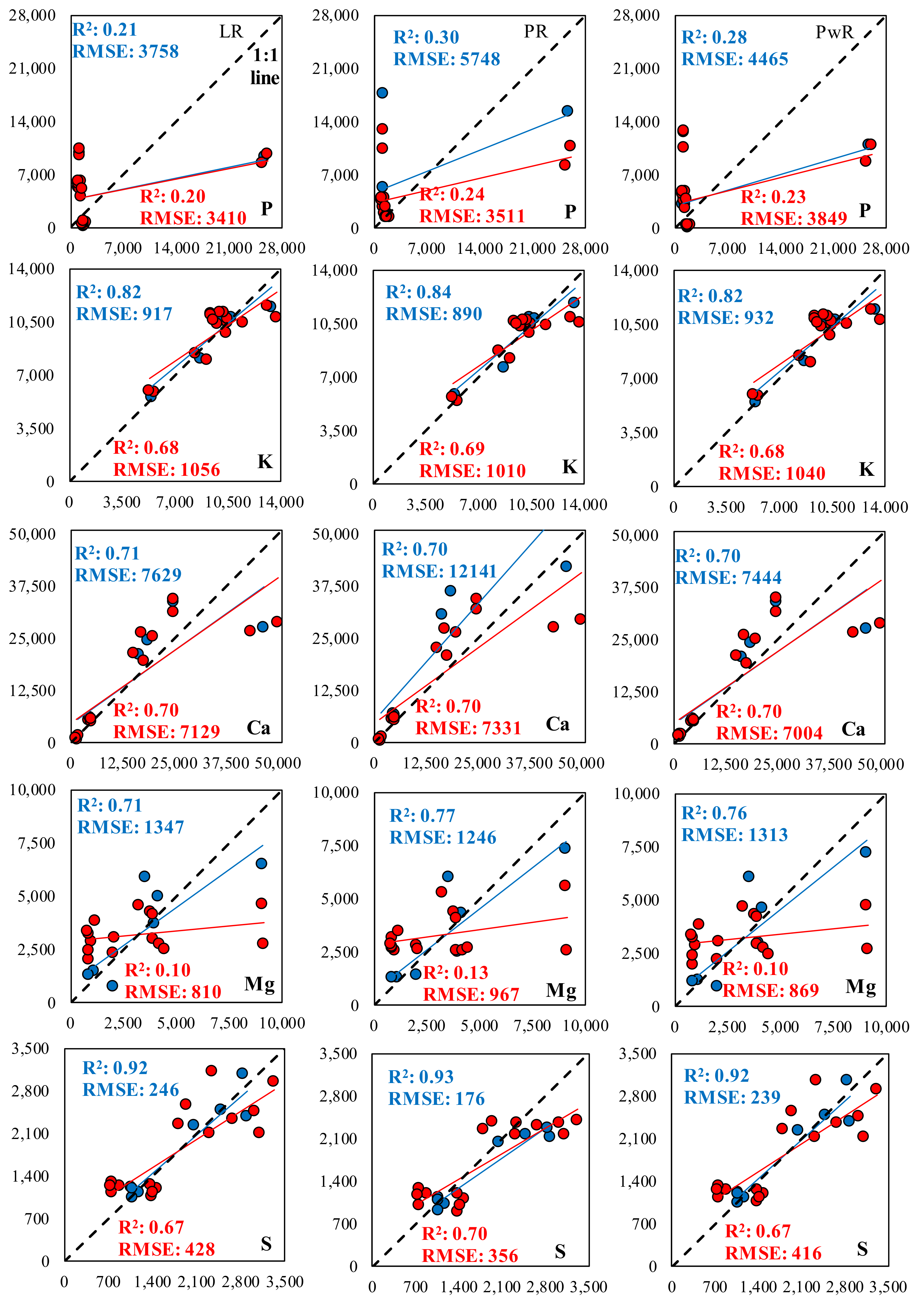
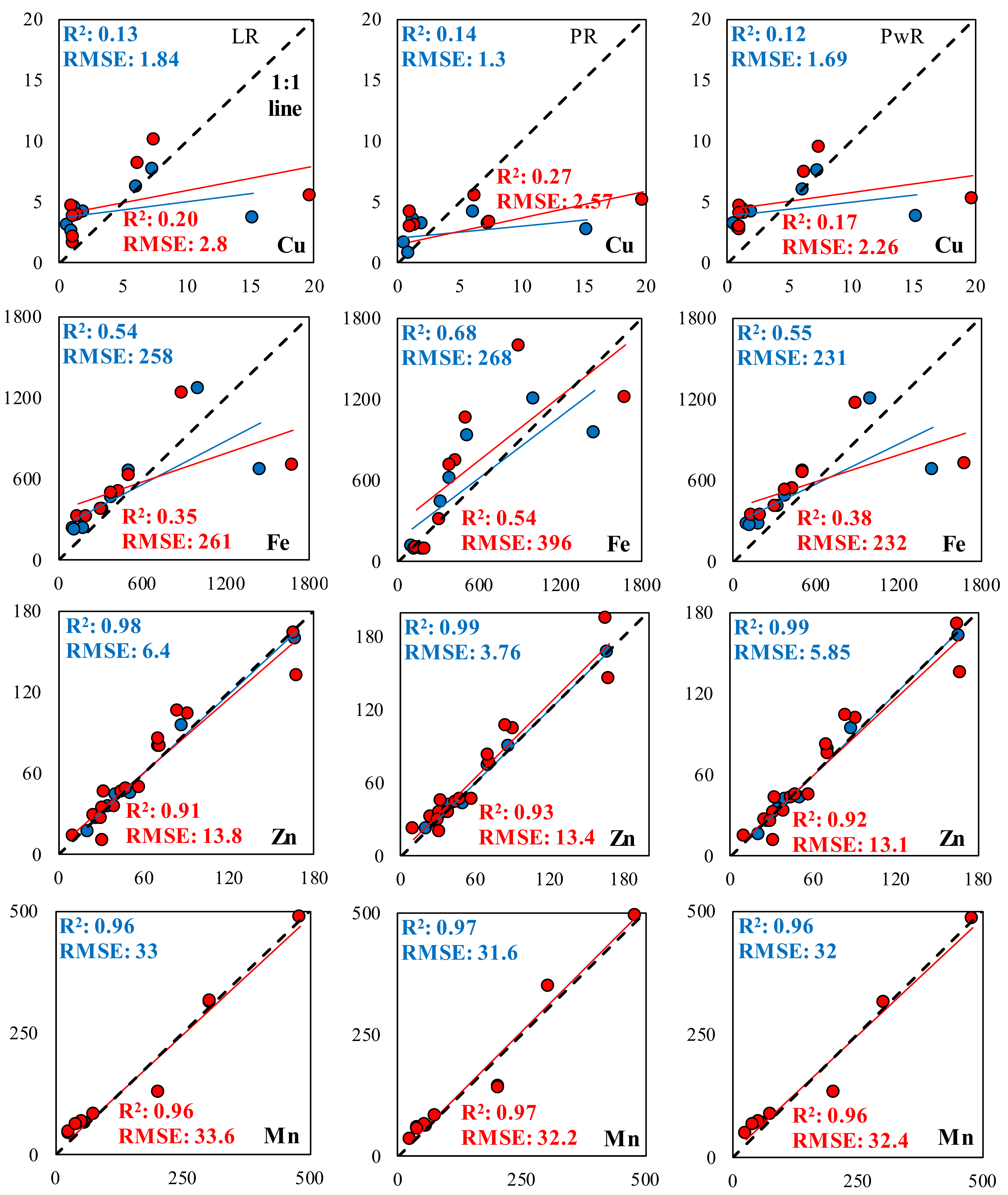
RMSE—root mean square error; NRMSE—normalized RMSE; MAE—mean absolute error; RPD—residual prediction deviation; LR—linear regression; PR—polynomial regression; PwR—power regression; R²—coefficient of determination. Regression models are significant at * p < 0.05, ** p < 0.01, and *** p < 0.001, or are not significant ^NS at p > 0.05.

presents the statistical parameters of regression models used for the prediction of plant nutrient concentrations based on pXRF data via LR, PR, PwR, and their respective R² values. Although all models can be reliable to predict Ca and Fe concentrations, the PwR provided better root mean square error (RMSE) values (Table 4), which is further evidenced in Figure 1, or in Figure 2, when including an independent dataset of measurements. Very high correlations were found between data provided by the pXRF probe and K, S, Zn, and Mn wet chemistry, regardless of the model tested. This is further illustrated in Figure 1; Figure 2 when establishing the relationship between observed and predicted values, where data points are more homogeneously distributed along the 1:1 line. As for Mg, although relationships were less strong, all models provided a good relationship at the same magnitude, at least for the ‘modeling’ dataset. Conversely, none of the regression models were able to establish adequate relations for P and Cu (Table 4 and Figure 1; Figure 2).

In addition to the ‘modeling’ dataset that was used to predict nutrient concentration in plant samples, a completely independent dataset of measurements was included for each regression model, as demonstrated in Figure 1; Figure 2. This has further reinforced the validation and reliability of measurements via the pXRF probe using the ‘Soil Nutrient and Metal’ calibration of the probe, mainly to determine the concentration of K, S, Zn, and Mn in plant samples, since relationships remained strong for the independent samples. Such a dataset was ensured to fall into the concentration range of the ‘modeling’ dataset, as measured by the standard method of acid digestion, and the same approach has been used by Pelegrino et al. [6] in another study using a pXRF probe for agricultural purposes.

4. Discussion

The evaluation of the accuracies and errors of the models is presented in Table 4 (1:1 graphs, between observed and predicted values, are shown in Figure 1; Figure 2). The lowest RMSE value was used as a criterion for selecting the best model for each nutrient’s prediction. According to the data obtained in each model tested, it was observed that for the prediction of Ca and Fe, the best model was the PwR, although LR also presented good results.

According to the statistical analyses of the regressions (Table 4), no model was able to accurately predict P and Cu when using pXRF data. Therefore, to establish reliable correlations with P and Cu contents, further evaluation with other auxiliary variables and different approaches—such as data fusion with other proximal sensors—might become necessary, for example, an approach involving visible near-infrared diffuse reflectance spectroscopy (Vis-NIR) [14,15,16,17]. Moreover, those poor results for P and Cu warrant the evaluation of different models. For example, the use of a stepwise multiple linear regression model (SMLR) could consider all pXRF-reported elements used as independent variables for predicting the nutrient contents. Initially, such a model would incorporate all variables into the model, followed by the removal of the least important/interfering ones, then the remaining variables would constitute the final SMLR. In our experiment, such a model was not evaluated because the ‘Soil Nutrient and Metal’ calibration integrates a total of 47 elements. Among them, several elements are not usually encountered in plant samples; thus, either such elements would need to be replaced by ‘zero’ values, or those commonly present in both soils and plants must be used. This reinforces the need of developing a calibration method for ‘Plant and Soil’, that could cover potential elements present in both materials. However, the use of easier and more accessible models, such as those tested in our experiment, would be more feasible in practice.

Another reason behind the poor measurements of P could be the fact that the maximum concentration found in plants was much higher than the maximum concentration of P in the ‘Soil Nutrient and Metal’ calibration method, even for the ‘modeling’ dataset (Table 2 and Supplementary Table S1); conversely, Cu measurements are within the concentration range of the pXRF probe and provided inadequate predictions (Table 2 and Supplementary Table S1). Additionally, Ca predictions were quite reliable although maximum values were also higher than the maximum concentration in the soil method. Interestingly, in the case of Mg, the independent dataset did not agree with the ‘modeling’ dataset, even when all values were falling into the concentration range of pXRF. These slight drawbacks in the results—with the additional considerations of the interference of auxiliary variables and the fusion of data from multiple proximal sensors—emphasize the importance of defining other prediction models for practical applications and decision making.

For plant samples collected across Oklahoma, US, the net intensities from a pXRF probe can be used to reliably predict the concentration of most elements, such as K, S, Zn, and Mn. For this, the simple linear equations showed in Table 3 can be used. For practicability, Ca and Fe do not require the use of PwR for nutrient concentration predictions (the use of PwR is only needed if higher accuracy is required); thus, equations presented in Table 3 can be used as well. Other regression models were tested, since P and Cu provided very poor linear predictions; however, neither of them succeeded in better predicting their concentrations via a pXRF probe.

For our instrument, since a calibration method of a pXRF probe covered the plant and soil nutrient concentrations, reliable measurements and predictions can be used for both materials. Some refinements would be encouraged in the development of such a calibration method, taking into account the many matrixes and heterogeneities of the different samples. Worst case scenario, soil and plant samples must only be processed, and no acid digestion is required to analyze either total soil nutrient contents or plant nutrient contents, if a pXRF probe is used. In that case, samples would skip the wet chemical digestion involved and would undergo measurements directly from the process. In addition, a positive scenario of measuring samples onsite can be encouraged, since recent literature has shown positive results of a pXRF probe’s measurements on fresh leaves [4]. In this context, studies of environmental concern would be capable of measuring potentially toxic metals (PTMs) in soils in situ, while at the same time measuring the uptake of PTMs by plants—either native or cultivated (for phytoremediation purposes)—using a single calibration method of a pXRF probe. For agricultural purposes, the same could be done for accessing nutrient uptake by plants in order to correlate them with the exchangeable contents of those nutrients in the soil, which can be also predicted from a pXRF probe [6].

References

- McLaren, T.I.; Guppy, C.N.; Tighe, M.K. A rapid and nondestructive plant nutrient analysis using portable X-ray fluorescence. Soil Sci. Soc. Am. J. 2012, 76, 1446–1453. [Google Scholar] [CrossRef]
- Towett, E.K.; Shepherd, K.D.; Lee Drake, B. Plant elemental composition and Portable X-ray Fluorescence (pxrf) spectroscopy: Quantification under different analytical parameters. X-ray Spectrom. 2016, 45, 117–124. [Google Scholar] [CrossRef] [Green Version]
- Sapkota, Y.; McDonald, L.M.; Griggs, T.C.; Basden, T.J.; Drake, B.L. Portable X-ray fluorescence spectroscopy for rapid and cost-effective determination of elemental composition of ground forage. Front. Plant Sci. 2019, 10, 317. [Google Scholar] [CrossRef] [PubMed] [Green Version]
- Costa, G.T., Jr.; Nunes, L.C.; Feresin Gomes, M.H.; Almeida, E.; de Carvalho, H.W.P. Direct determination of mineral nutrients in soybean leaves under vivo conditions by portable x-ray Fluorescence Spectroscopy. X-ray Spectrom. 2020, 49, 274–283. [Google Scholar]
- Kalra, Y.P. Handbook of Reference Methods for Plant Analysis; CRC Press: Boca Raton, FL, USA, 2019. [Google Scholar]
- Pelegrino, M.H.; Silva, S.H.; de Faria, Á.J.; Mancini, M.; Teixeira, A.F.; Chakraborty, S.; Weindorf, D.C.; Guilherme, L.R.; Curi, N. Prediction of soil nutrient content via pXRF spectrometry and its spatial variation in a highly variable tropical area. Precis. Agric. 2021, 22, 1–17. [Google Scholar]
- Reidinger, S.; Ramsey, M.H.; Hartley, S.E. Rapid and accurate analyses of silicon and phosphorus in plants using a portable X-ray Fluorescence Spectrometer. New Phytol. 2012, 195, 699–706. [Google Scholar] [CrossRef] [PubMed]
- Zhang, H.; Antonangelo, J.; Penn, C. Development of a rapid field testing method for metals in horizontal directional drilling residuals with XRF sensor. Sci. Rep. 2021, 11, 3901. [Google Scholar] [CrossRef] [PubMed]
- Westerman, R.L. Soil Testing and Plant Analysis; Soil Science Society of America: Madison, WI, USA, 1990. [Google Scholar]
- Willmott, C.J.; Ackleson, S.G.; Davis, R.E.; Feddema, J.J.; Klink, K.M.; Legates, D.R.; O’Donnell, J.; Rowe, C.M. Statistics for the evaluation and comparison of Models. J. Geophys. Res. 1985, 90, 8995. [Google Scholar] [CrossRef] [Green Version]
- Chang, C.-W.; Laird, D.A.; Mausbach, M.J.; Hurburgh, C.R. Near-infrared reflectance spectroscopy-principal components regression analyses of soil properties. Soil Sci. Soc. Am. J. 2001, 65, 480–490. [Google Scholar] [CrossRef] [Green Version]
- Peng, J.-L.; Kim, M.-J.; Jo, M.-H.; Min, D.-H.; Kim, K.-D.; Lee, B.-H.; Kim, B.-W.; Sung, K.-I. Accuracy evaluation of the crop-weather yield predictive models of Italian ryegrass and forage rye using cross-validation. J. Crop Sci. Biotechnol. 2017, 20, 327–334. [Google Scholar] [CrossRef]
- Rinaldi, M.; Losavio, N.; Flagella, Z. Evaluation and application of the OILCROP–sun model for sunflower in southern Italy. Agric. Syst. 2003, 78, 17–30. [Google Scholar] [CrossRef]
- Andrade, R.; Silva, S.H.; Faria, W.M.; Poggere, G.C.; Barbosa, J.Z.; Guilherme, L.R.; Curi, N. Proximal sensing applied to soil texture prediction and mapping in Brazil. Geoderma Reg. 2020, 23, e00321. [Google Scholar] [CrossRef]
- Benedet, L.; Acuña-Guzman, S.F.; Faria, W.M.; Silva, S.H.; Mancini, M.; Teixeira, A.F.; Pierangeli, L.M.; Acerbi Júnior, F.W.; Gomide, L.R.; Pádua Júnior, A.L.; et al. Rapid soil fertility prediction using x-ray fluorescence data and machine learning algorithms. CATENA 2021, 197, 105003. [Google Scholar] [CrossRef]
- Chatterjee, S.; Hartemink, A.E.; Triantafilis, J.; Desai, A.R.; Soldat, D.; Zhu, J.; Townsend, P.A.; Zhang, Y.; Huang, J. Characterization of field-scale soil variation using a stepwise multi-sensor fusion approach and a cost-benefit analysis. CATENA 2021, 201, 105190. [Google Scholar] [CrossRef]
- Vasques, G.M.; Rodrigues, H.M.; Coelho, M.R.; Baca, J.F.; Dart, R.O.; Oliveira, R.P.; Teixeira, W.G.; Ceddia, M.B. Field proximal SOIL sensor fusion for Improving High-resolution Soil Property Maps. Soil Syst. 2020, 4, 52. [Google Scholar] [CrossRef]
Figure 1.
The relationship between the observed (x-axis) and predicted values (y-axis), shown in mg kg−1, of the nutrient contents (P, K, Ca, Mg, and S) of plant samples. RMSE—root mean square error. The observed values are the actual values obtained, and the predicted values are the values of the variable predicted, based on the regression analysis. Blue and red points are ‘modeling’ and independent (‘validation’ samples) datasets of measurements, respectively. Black dashed lines represent the 1:1 line, and blue and red solid lines represent the actual regression curves from the ‘modeling’ and ‘independent’ datasets, respectively.
Figure 2.
The relationship between observed (x-axis) and predicted values (y-axis), shown in mg kg−1, of the nutrient contents (Cu, Fe, Zn, and Mn) of plant samples. RMSE—root mean square error. The observed values are the actual values obtained, and the predicted values are the values of the variable predicted, based on the regression analysis. Blue and red points are ‘modeling’ and independent (‘validation’ samples) datasets of measurements, respectively. Black dashed lines represent the 1:1 line, and blue and red solid lines represent the actual regression curves from the ‘modeling’ and ‘independent’ datasets, respectively.