Article

Impacts of Biomass Burning Emission Inventories and Atmospheric Reanalyses on Simulated PM10 over Indochina

1
Graduate School of Engineering, Osaka University, 2-1 Yamadaoka, Suita, Osaka 565-0871, Japan
2
Environmental Engineering Department, KANSO CO., LTD., 1-3-5 Azuchimachi, Osaka Chuo-ku, Osaka 541-0052, Japan
*
Author to whom correspondence should be addressed.
Submission received: 19 December 2019 / Revised: 19 January 2020 / Accepted: 24 January 2020 / Published: 4 February 2020

Abstract

:
Biomass burning (BB) is a major source of atmospheric particles over Indochina during the dry season. Moreover, Indochina has convoluted meteorological scales, and regional meteorological conditions dominate the transport patterns of pollutants. This study focused on the impacts of BB emission inventories and atmospheric reanalyses on simulated PM10 over Indochina in 2014 using the Community Multiscale Air Quality (CMAQ) model. Meteorological fields to input to CMAQ were produced by using the Weather Research and Forecasting (WRF) model simulation with the United States National Centers for Environmental Prediction Final (NCEP FNL) Operational Global Analysis or European Centre for Medium Range Weather Forecasts Interim Reanalysis (ERA-interim). The Fire INventory from NCAR (FINN) v1.5 or the Global Fire Emissions Database including small fires (GFED v4.1s) was selected for BB emissions for the air quality simulation. The simulation case with NCEP FNL and FINN v1.5 (FNL + FINN) performed best throughout 2014, including the season when BB activities were intensified. The normalized percentage difference for maximum daily mean PM10 concentrations at Chiang Mai for FNL + FINN and the two simulation cases applying GFED v4.1s for BB emissions (−53% to −27%) was much larger than that between the FNL + FINN and ERA + FINN cases (10%). BB emission inventories more strongly impacted PM10 simulation than atmospheric reanalyses in highly polluted areas by BB over Indochina in 2014.

1. Introduction

Indochina, the peninsular region that includes Cambodia, Laos, Myanmar, Thailand, and Vietnam, has a monsoonal climate with a dry and wet season; the prevailing wind direction and the pattern of precipitation changes seasonally. During the dry season, particulate pollution degrades air quality over Indochina [1]. Outdoor exposure to particulate matter (PM) contributes to ill health, such as cardio- and cerebrovascular disease, respiratory illnesses, lung cancer, and possibly other diseases [2]. A major source of atmospheric particles over Indochina is biomass burning (BB), such as forest fires and agricultural burning. Thailand is surrounded by mountainous areas where BB frequently occurs in the dry season. Chiang Mai, the largest city in northern Thailand, has experienced severe air pollution caused by BB [3,4,5]. Furthermore, measurements of aerosol properties on Dongsha Island in the northeastern South China Sea revealed that smoke originating from BB in Indochina rises and is trapped within the free troposphere (3–4 km above the earth’s surface) in some situations [5,6,7].
As part of NASA’s 2006 Biomass Burning Aerosols in Southeast Asia: Smoke Impact Assessment (BASE-ASIA), regional modeling studies were conducted to assess the impacts of BB in Southeast Asia on atmospheric composition over Asia in 2006 by using the Community Multiscale Air Quality (CMAQ) model [8]. The CMAQ simulations revealed that during two intense episodes in 2006, BB contributed to ground-level CO, O3, and PM2.5 concentrations in the source region of Southeast Asia by as much as 400 ppbv, 20 ppbv, and 80 µg m−3, respectively [9]. The emissions from BB could also be spread over the southeastern parts of East Asia via strong eastward transport in the free troposphere from 2 to 8 km above the earth’s surface [9,10]. It should be noted that the model performance was evaluated using only observed CO concentrations in Thailand, and that discrepancy existed between simulations and measurements due to uncertainty in emission inventories. Amnuaylojaroen et al. [11] reported that BB emissions create a substantial increase for simulated O3 and CO surface mixing ratios by up to 29% and 16%, respectively, for Southeast Asia in 2008. However, particulate matter was not evaluated in the simulations. Li et al. [12] reported that BB contributed 70%–80% of simulated PM2.5 in northern Myanmar, Laos, and Vietnam during March-April 2013.
Several BB emission inventories are available, such as the Fire INventory from NCAR (FINN) [13], the Global Fire Assimilation System (GFAS) [14], and the Global Fire Emissions Database (GFED) [15]. BB emission inventories have substantial uncertainties in their temporal and spatial variabilities because the data to estimate the emissions of BB, such as area, fuel loading, and emission factors, are limited [13,15]. Vongruang et al. [16] reported that PM10 was overestimated in air quality simulation with FINN, whereas PM10 was underestimated with GFAS in the source region of Northern Thailand in March 2012.
Indochina has convoluted meteorological scales, and regional meteorological conditions dominate the transport patterns of pollutants [1]. Atmospheric reanalyses, initial and boundary conditions for a mesoscale model, have great impacts on the simulated meteorological fields. Several atmospheric reanalyses have been developed by different organizations, for example, the European Centre for Medium Range Weather Forecasts (ECMWF) Interim Reanalysis (ERA-interim) [17], the Japanese 55-year Reanalysis (JRA-55) [18] from the Japan Meteorological Agency (JMA), and the United States National Centers for Environmental Prediction Final (NCEP FNL) [19] Operational Global Analysis. These reanalyses employ various forecast models and data assimilation approaches. ERA-Interim has the highest ability to reproduce climate variables of the East Asian summer monsoon, especially precipitation [20,21].
To the best of our knowledge, there are few studies simulating particulate pollution in Indochina for a period of one year that consider the uncertainties of BB emissions and the complexities of the regional meteorology. In one study, two BB emission inventories were assessed by simulating particulate matter using CMAQ during a specific pollution event [16]. This study focused on the impacts of BB emission inventories and atmospheric reanalyses on the simulation of PM10 over Indochina in 2014. From the end of February to early April in 2014, agricultural burning and forest fires in northern Thailand caused severe particulate pollution over the region [5].

2. Materials and Methods

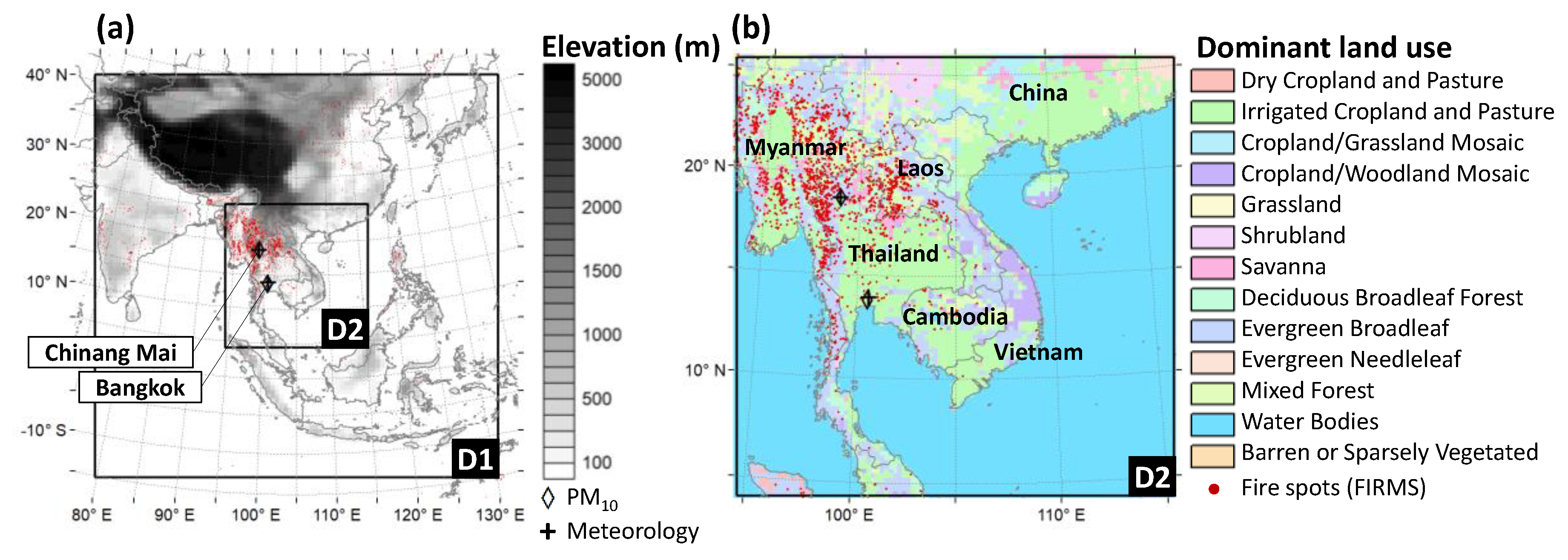
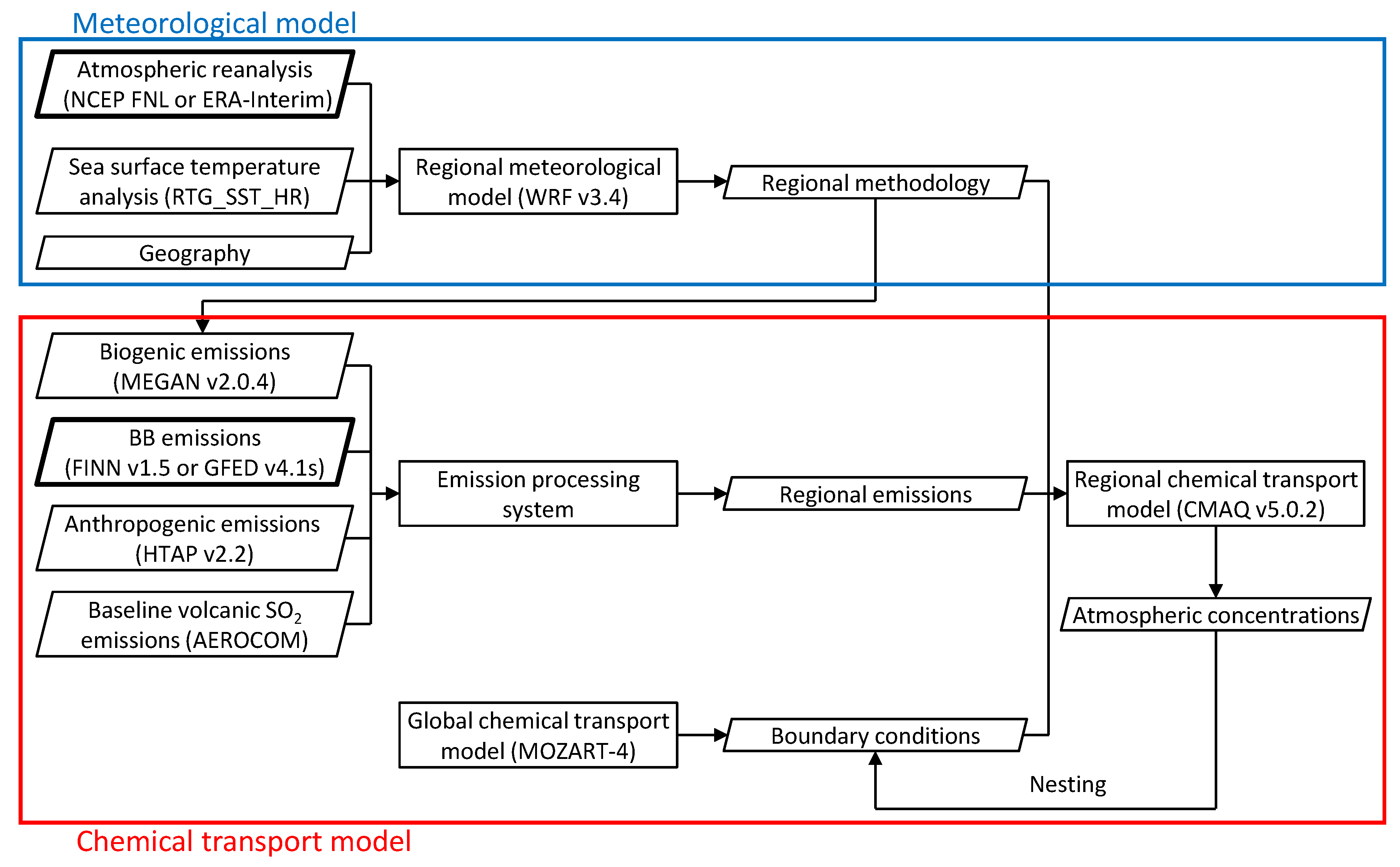
2.1. Simulation Design

Air quality simulations for the year 2014 were conducted by CMAQ v5.0.2 with an initial spin up period of December 2013. The modeling domains covered regions from East Asia (D1) to Indochina (D2) (Figure 1). The horizontal resolutions were 72 km and 24 km, and the number of grid cells were 92 × 92 and 98 × 98 for D1 and D2, respectively. The domains consisted of 30 sigma-pressure coordinate vertical layers ranging from the surface to 100 hPa. Figure 2 shows the procedure of air quality simulation in this study.

2.2. Meteorological Model

Meteorological fields to input to CMAQ were produced by using the Weather Research and Forecasting (WRF) model [22] v3.4. The WRF simulations were conducted using the high-resolution, real-time, global sea surface temperature analysis (RTG_SST_HR) of NCEP, and two atmospheric reanalyses: NCEP FNL or ERA-Interim. The physics options were as follows: Rapid Radiative Transfer Model for General Circulation Models Shortwave and Longwave Schemes [23], planetary boundary layer physics of Asymmetric Convection Model 2 Scheme [24], cumulus parameterization of the Kain–Fritsch Scheme [25], micro physics of Morrison 2-moment Scheme [26], and Pleim–Xiu Land Surface Model [27]. Grid nudging was applied to horizontal wind components at all the vertical layers with a coefficient of 3.0 × 10⁻⁴ s−1 in D1 and 1.0 × 10⁻⁴ s−1 in D2 for the entire period.

2.3. Chemical Transport Model

CMAQ was configured with the Carbon Bond chemical mechanism (CB05) [28] for gas-phase chemistry and the sixth generation CMAQ aerosol module for the aerosol process. The initial and lateral boundary conditions for D1 were obtained from the Model for Ozone and Related Chemical Tracers v4 (MOZART-4) [29]. Several datasets were used to produce emission data. In particular, the Fire INventory from NCAR (FINN) [11] v1.5 or the Global Fire Emissions Database including small fires (GFED v4.1s) [30] was selected for BB emissions. FINN v1.5 provided 1 km-resolution BB emissions estimated from the active fire observations from the Moderate Resolution Imaging Spectroradiometer (MODIS) Terra and Aqua satellite. GFED v4.1s provided 0.25°-resolution BB emissions estimated from the 500 m Collection 5.1 MODIS direct broadcast burned area product plus additional burned area from small fires based on a revised version of the Randerson et al. [31] small-fire estimation approach. Anthropogenic emissions were obtained from the Task Force Hemispheric Transport of Air Pollution (HTAP) v2.2 inventory [32]. The other natural emissions were derived from the Model of Emissions of Gases and Aerosols from Nature (MEGAN) [33] v2.04 for biogenic emissions and the Aerosol Comparisons between Observations and Models (AEROCOM) data [34] for baseline volcanic SO2 emissions. There were differences between the periods of simulations and the reference years in the anthropogenic emission data available for the simulations, and the uncertainties associated with the differences may have affected model performance.
In order to evaluate the impacts of BB emission inventories and atmospheric reanalyses on simulated PM10 concentrations, four cases of simulations (FNL + FINN; FNL + GFED; ERA + FINN; and ERA + GFED) were executed. The first parts of cases’ names indicate the applied reanalysis: FNL and ERA stand for NCEP FNL and ERA-Interim, respectively. The second parts indicate the selected BB emission inventories. Furthermore, simulations without BB emission inventories (FNL + exBB; ERA + exBB) were conducted. The difference between cases with BB emissions and those without BB emissions was calculated to estimate BB contributions to PM10 concentrations in the four simulation cases with BB emissions.
Figure 3 shows spatial distributions of PM10 emissions from FINN v1.5 and GFED v4.1s in March and April 2014. During these two months, PM10 emissions in both BB emission inventories were concentrated in Indochina, especially the mountainous areas in Laos, Myanmar, and Thailand. FINN v1.5 estimated larger emissions in a wider area than GFED v4.1s. Figure 4 shows the variation of the amount of PM10 emissions over D2 and the relative contributions from BB. PM10 emissions from BB produced by FINN v1.5 and GFED v4.1s accounted for 244 mg s−1 km−2 and 91 mg s−1 km−2, respectively, which contributed 93% and 83%, respectively, of the total amount of PM10 emissions in March when burning activities were intensified.
The WRF performance was evaluated through comparison with ground-level air temperature, relative humidity, and wind speed data in Bangkok and Chiang Mai distributed by the University of Wyoming [35]. The CMAQ performance was evaluated through comparison with ground-level PM10 concentration data in Bangkok and Chiang Mai distributed by the Acid Deposition Monitoring Network in East Asia (EANET) [36].

3. Results

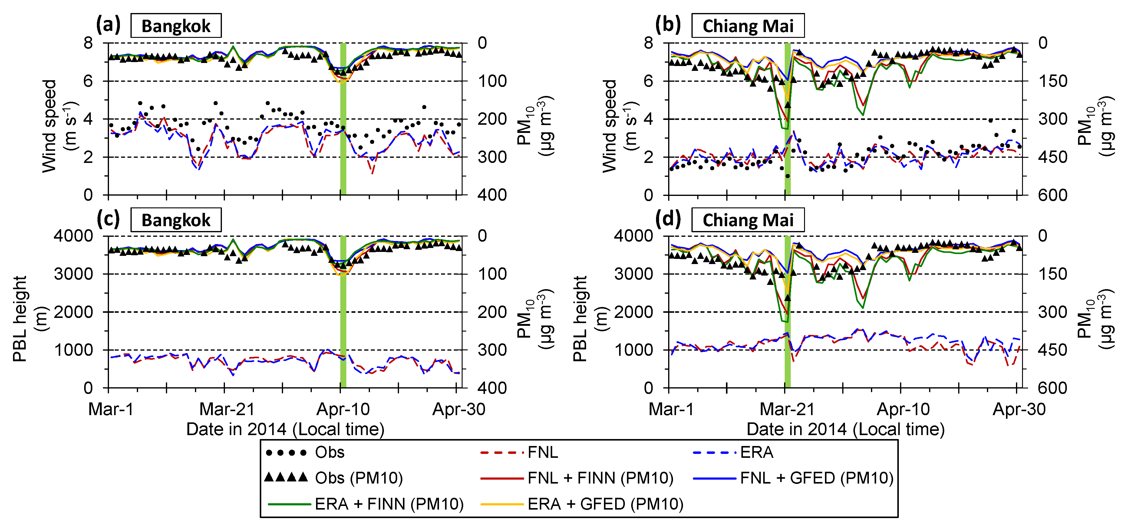
3.1. Daily Meteorological Factors at Observation Sites

The WRF performance was evaluated by using the normalized mean bias (NMB) and the index of agreement (IA) for ground-level air temperature, relative humidity, and wind speed for Bangkok and Chiang Mai (Table 1). More statistics were shown in supplementary data (Table S1). IA is a statistical measure to present the model performance and varies between 0 and 1, where 1 means model performance is perfect [37]. IA values for air temperature, relative humidity, and wind speed were relatively high in both WRF simulations: the models applying both NCEP FNL and ERA-interim simulated spatial and temporal variations of these parameters in the same level.

3.2. Daily Concentrations of PM10 at Observation Sites

The performance of daily mean PM10 concentration simulations in the four simulation cases with BB emissions was evaluated by using NMB and IA for the periods of both the entire year and the two month period from March to April 2014 (Table 2). More statistics were shown in supplementary data (Table S2). The highest PM10 concentrations in 2014 were observed on January 3 at Bangkok (123.9 µg m−3) and on March 21 at Chiang Mai (242.9 µg m−3), respectively. At Chiang Mai, maximum daily mean PM10 concentrations were simulated in all of the four simulation cases on the same day: March 21. The IA value for FNL + FINN was the highest for both the one-year and the two-month periods, indicating that FNL + FINN performed best throughout 2014, including the season when BB activities were intensified.
Figure 5 shows simulated and observed daily concentrations at Bangkok and Chiang Mai. All of the four simulation cases simulated the day-to-day variation patterns well at both sites for the year 2014. Cases applying FINN v1.5 for BB emissions (FNL + FINN; ERA + FINN) showed higher trends of simulated PM10 concentrations at both observation sites compared to those applying GFED v4.1s (FNL + GFED; ERA + GFED), regardless of the atmospheric reanalysis. In particular, the former two cases clearly presented higher trends of PM10 concentrations than the latter cases at Chiang Mai from the end of February to early April, when high PM10 concentrations were observed. Table 3 shows the normalized percentage difference for FNL + FINN and the other three cases for annual mean and maximum daily mean PM10 concentrations in 2014 at the two observation sites. The percentage difference at Bangkok (−9% to −4% for annual mean; −15% to −2% for maximum) was less than that at Chiang Mai (−19%–8% for annual mean; −53%–10% for maximum). At both of the two sites, the percentage difference between the FNL + FINN and ERA + FINN cases was the smallest for annual mean and maximum daily mean PM10 concentrations in 2014. In particular, the difference for maximum daily mean PM10 concentrations at Chiang Mai for FNL + FINN and the two cases applying GFED v4.1s for BB emissions (−53% to −27%) was much larger than that between the FNL + FINN and ERA + FINN cases (10%). Consequently, BB emission inventories more strongly impacted the PM10 simulation than atmospheric reanalyses at the two sites in Indochina.
BB contributions were estimated by the difference between cases with and without BB emissions (Figure 5). The BB contributions to PM10 concentrations of the four simulation cases were 2%–12% at Bangkok and 75%–89% at Chiang Mai for each day that the maximum concentrations were observed. Li et al. [12] reported that BB contributions to simulated PM2.5 was 70%–80% in the BB source regions during March-April 2013 and the contributions were close to 75%–89% at Chiang Mai on 21 March 2014.
Figure 6 shows simulated and observed wind speed, planetary boundary layer (PBL) height, and daily concentrations at Bangkok and Chiang Mai from March to April. At Bangkok, these parameters were on the similar trends among the four simulation cases. At Chiang Mai, the maximum PM10 concentration was observed in weak-wind condition. On the other hand, there was little relationship between PBL height and PM10 concentrations. The simulated spatial distributions on January 3 and March 21 are analyzed in detail in the next subsection.

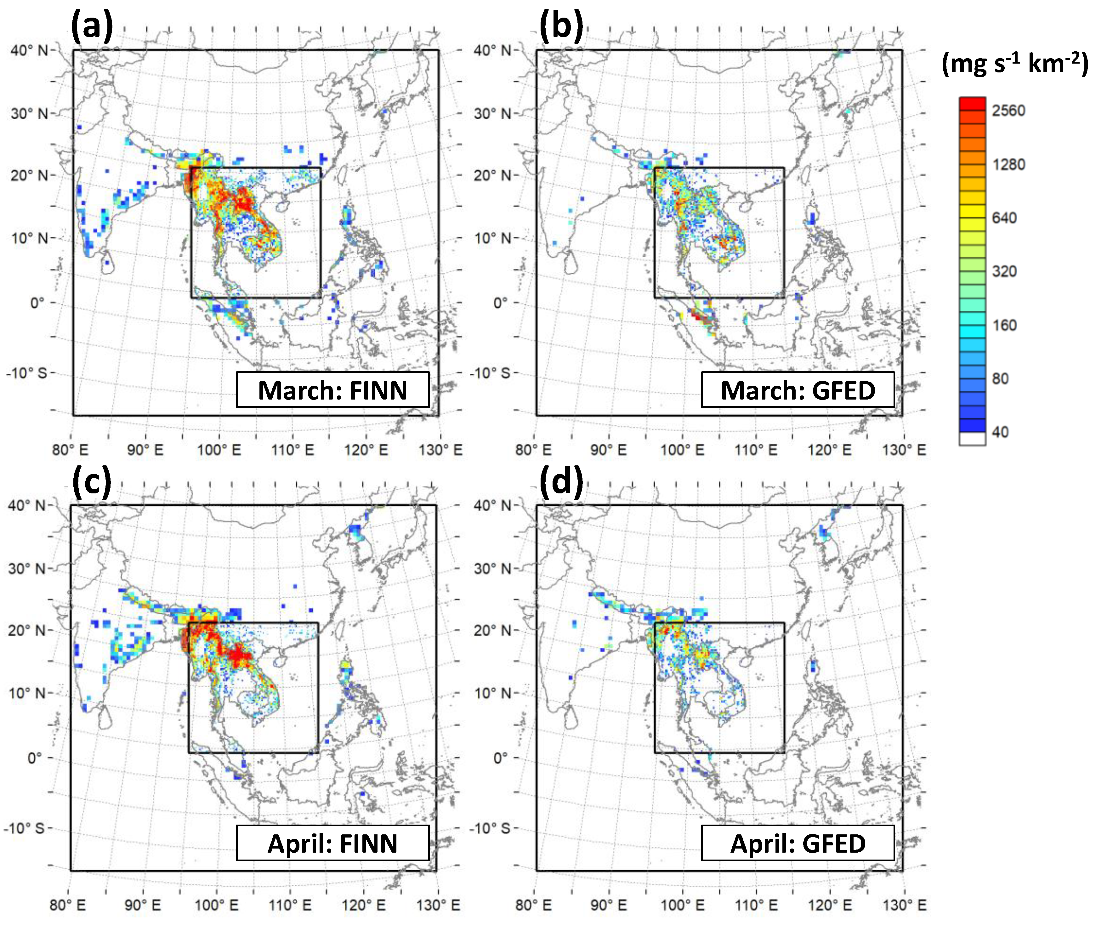
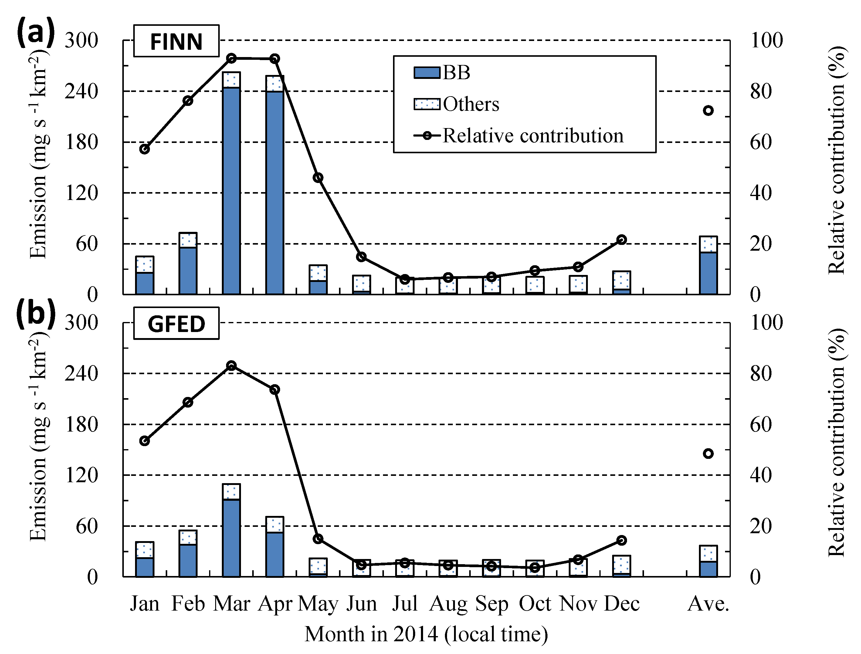
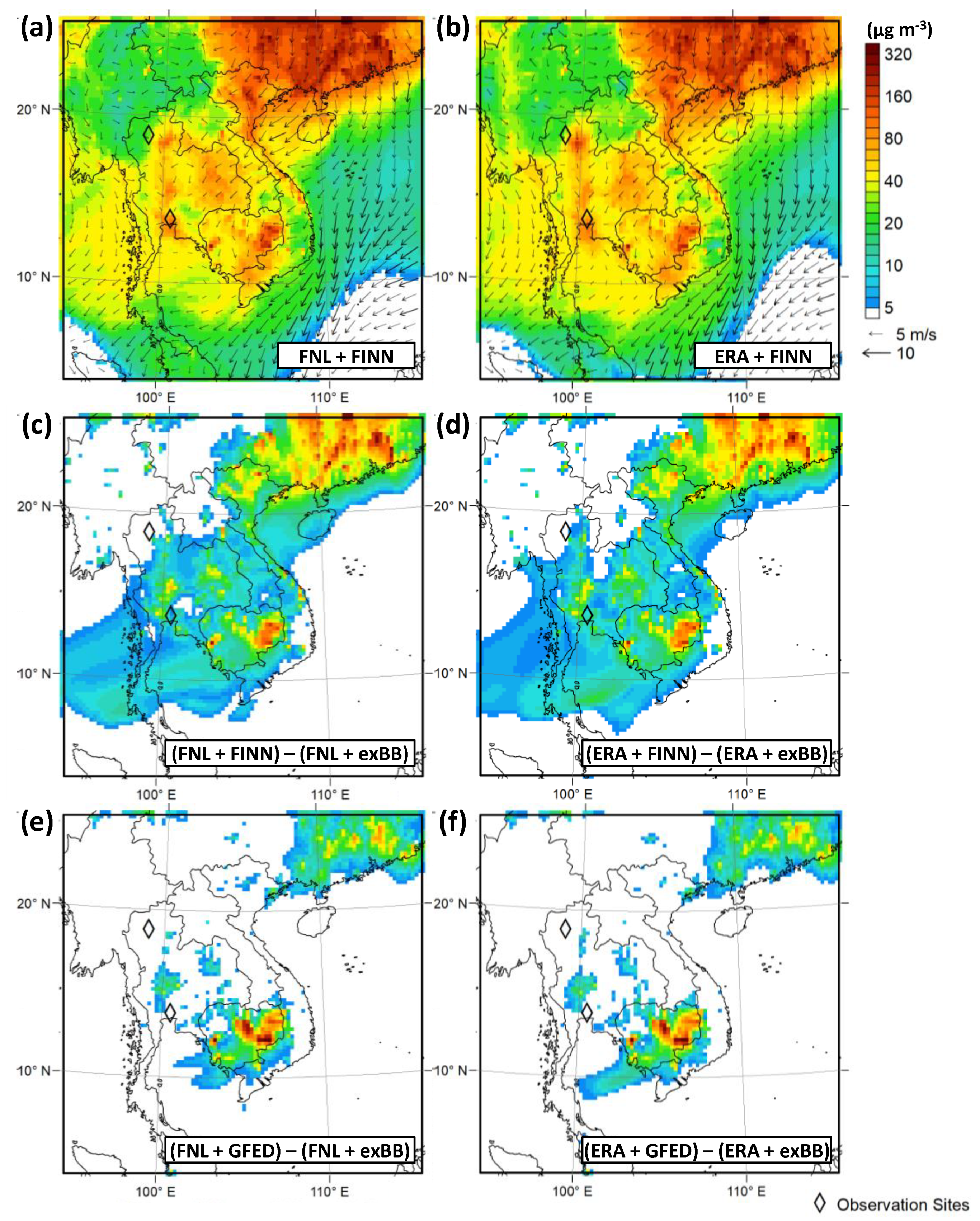
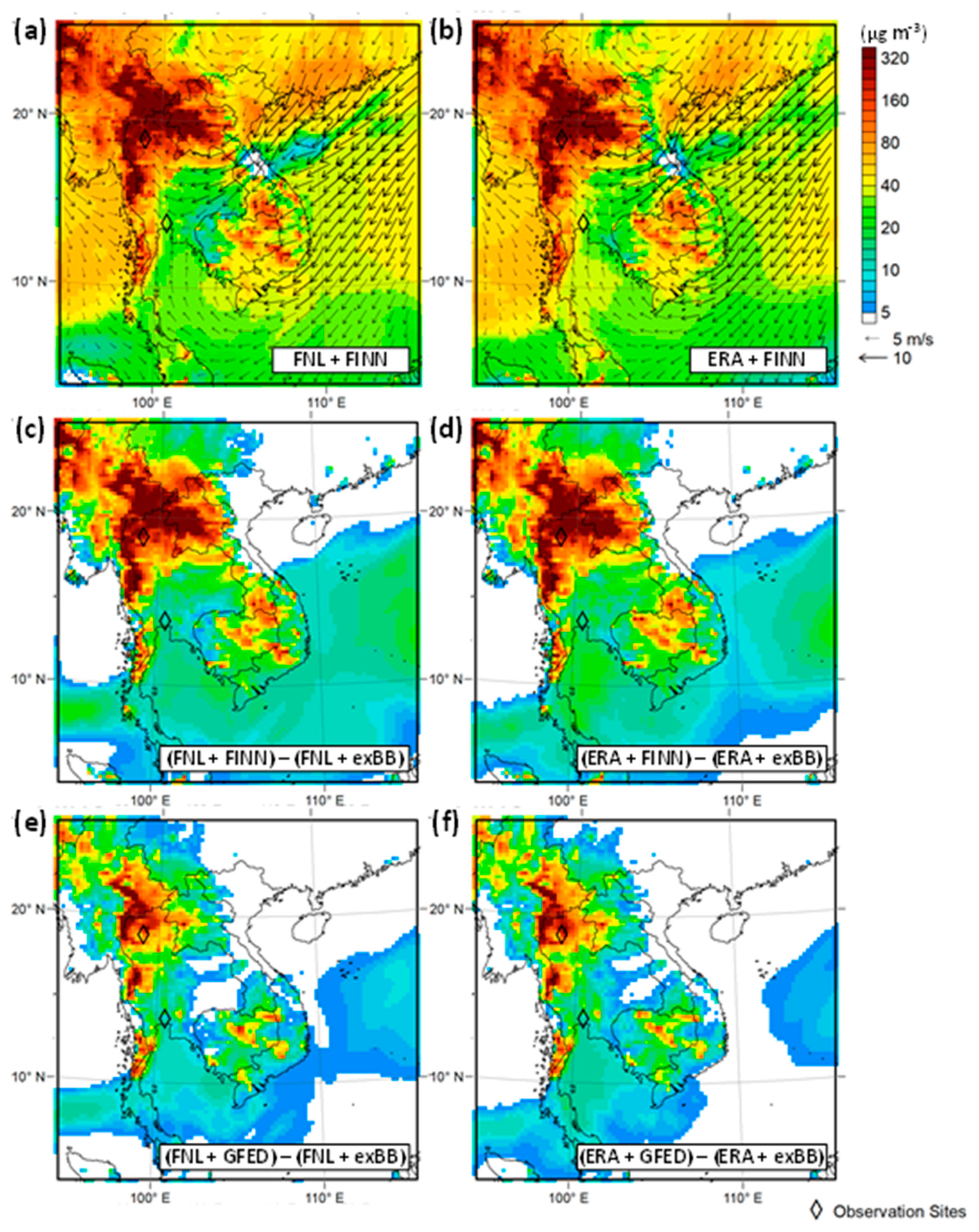
3.3. Spatial Distributions for Daily Concentrations of PM10

Figure 7 shows the spatial distributions of daily PM10 concentrations and wind fields at ground level on January 3, when maximum PM10 concentration was observed in Bangkok. The large BB contribution area was spread out over Southern China and Cambodia. On January 3, ground-level winds were weak over Indochina. The area where simulated PM10 concentrations were around 80 µg m−3 was spread across Thailand, and the BB contributions were relatively small in the four cases; discrepancy among the four cases was small across Thailand.
In March 2014, the largest number of hotspots were detected in Thailand and Myanmar from March 18 to 21 [5]. A large number of fire spots occurred in the mountainous areas of Indochina on March 21 (Figure 1). Figure 8 shows spatial distributions of daily PM10 concentrations and wind fields at ground level on March 21. Ground-level winds blew easterly in the eastern part of Indochina and converged at the Myanmar and Thailand border in all cases. Concentrations of 160 µg m−3 of PM10 were spread over the area along the Myanmar and Thailand border in the four cases with BB emissions; the two cases that FINN v1.5 selected for BB emissions were predicted to have higher PM10 concentrations in and around Northern Laos. In highly polluted areas caused by BB over Indochina, the discrepancy of simulated PM10 concentrations resulting from different BB emission inventories was larger than that resulting from different atmospheric reanalyses.

4. Conclusions

This study focused on the impacts of BB emission inventories and atmospheric reanalyses on the simulation of PM10 over Indochina for the year 2014. Meteorological fields to input to CMAQ were produced by using the WRF model simulation with NCEP FNL or ERA-interim. FINN v1.5 or GFED v4.1s were selected for BB emissions. In order to evaluate the impacts, four cases of simulations (FNL + FINN; FNL + GFED; ERA + FINN; ERA + GFED) were executed.
The performance of CMAQ simulations for PM10 concentrations at ground-level was evaluated at Bangkok and Chiang Mai in Thailand. The FNL + FINN case performed best for both the full year and the two-month period when BB activities were intensified in 2014. To compare the impacts of input data (BB emission inventories and atmospheric reanalyses) on simulated PM10, we introduced the normalized percentage difference for FNL + FINN and the other three cases (FNL + GFED; ERA + FINN; ERA + GFED) for annual mean and maximum daily mean PM10 concentrations in 2014 at the two observation sites. At both of the two sites, the normalized percentage difference for annual mean and maximum daily mean PM10 concentrations in 2014 for FNL + FINN and the two cases applying GFED v4.1s for BB emissions (FNL + GFED; ERA + GFED) was larger than that between FNL + FINN and ERA + FINN cases. In particular, the difference for maximum daily mean PM10 concentrations at Chiang Mai for FNL + FINN and the two cases applying GFED v4.1s (−53% to −27%) was much larger than that between the FNL + FINN and ERA + FINN cases (10%).
BB contributions were estimated by the difference between the cases with BB emissions and those without BB emissions. BB contributions to PM10 concentrations in the four simulation cases at Chiang Mai (75%–89%) were larger than those at Bangkok (2%–12%) on the day when the highest PM10 concentrations were observed in 2014 at each observation site. BB highly contributed on the particulate pollution over Southern china and Cambodia on January 3, and over the area along the Myanmar and Thailand border on March 21 in weak-wind condition. In polluted areas caused by BB, the cases applying FINN v1.5 for BB emission inventories showed higher trends of PM10 concentrations. Selected BB emission inventories more strongly impacted the PM10 simulation than selected atmospheric reanalyses in highly polluted areas by BB over Indochina in 2014.
This approach is applicable to other years and atmospheric pollutants to evaluate the impacts of selected input datasets on air quality simulations in polluted areas caused by BB. For example, GFAS can be used for one of the other BB emission inventories. However, emission factors of global BB emission inventories, such as FINN, GFAS, and GFED, were determined based on generic vegetation types of each fire pixel. BB-emission data focusing on the unique characteristics of BB in the specific region would reduce the uncertainties of BB emissions. We hope that this study will help to improve understanding about the mechanisms that degrade air quality over Indochina.

Supplementary Materials

The following are available online at https://0-www-mdpi-com.brum.beds.ac.uk/2073-4433/11/2/160/s1, Table S1. Model performance for daily mean meteorological factors in the two simulation cases for the periods of one year and two months (from March to April) in 2014. Table S2. Model performance for daily mean PM10 concentrations in the four simulation cases for the periods of one full year (2014) and two months (from March to April 2014).

Author Contributions

Conceptualization, K.T., H.S., and A.K.; methodology, H.S. and K.U.; software, H.S. and K.U.; validation, K.T. and H.S.; formal analysis, K.T. and H.S.; data curation, H.S.; writing—original draft preparation, K.T.; writing—review and editing, H.S., K.U., and A.K.; visualization, K.T.; supervision, A.K.; project administration, H.S. All authors have read and agreed to the published version of the manuscript.

Funding

This research received no external funding.

Conflicts of Interest

The authors declare no conflict of interest.

References

  1. Reid, J.S.; Hyer, E.J.; Johnson, R.S.; Holben, B.N.; Yokelson, R.J.; Zhang, J.; Campbell, J.R.; Christopher, S.A.; Girolamo, L.D.; Giglio, L.; et al. Observing and understanding the Southeast Asian aerosol system by remote sensing: An initial review and analysis for the Seven Southeast Asian Studies (7SEAS) program. Atmos. Res. 2013, 122, 403–468. [Google Scholar] [CrossRef] [Green Version]
  2. IPCC. Climate Change 2014: Impacts, Adaptation, and Vulnerability. Part A: Global and Sectoral Aspects. Working Group II Contribution to the Fifth Assessment Report of the Intergovernmental Panel on Climate Change. Available online: https://www.ipcc.ch/report/ar5/wg2/ (accessed on 19 December 2019).
  3. Pengchai, P.; Chantara, S.; Sopajaree, K.; Wangkarn, S.; Tencharoenkul, U.; Rayanakorn, M. Seasonal variation, risk assessment and source estimation of PM 10 and PM10-bound PAHs in the ambient air of Chiang Mai and Lamphun, Thailand. Environ. Monit. Assess. 2009, 154, 197–218. [Google Scholar] [CrossRef] [PubMed]
  4. Tsai, Y.I.; Soparajee, K.; Chotruksa, A.; Wu, H.C. Source indicators of biomass burning associated with inorganic salts and carboxylates in dry season ambient aerosol in Chiang Mai basin, Thailand. Atmos. Environ. 2013, 78, 93–104. [Google Scholar] [CrossRef]
  5. Duc, H.N.; Bang, H.Q.; Quang, N.X. Modelling and prediction of air pollutant transport during the 2014 biomass burning and forest fires in peninsular Southeast Asia. Environ. Monit. Assess. 2016, 188, 106. [Google Scholar] [CrossRef] [PubMed]
  6. Atwood, S.A.; Reid, J.S.; Kreidenweis, S.M.; Cliff, S.; Zhao, Y.; Lin, N.-H.; Tsay, S.-C.; Chu, Y.-C.; Westphal, D.L. Size resolved measurements of springtime aerosol particles over the northern South China Sea. Atmos. Environ. 2013, 78, 134–143. [Google Scholar] [CrossRef]
  7. Wang, S.H.; Tsay, S.-C.; Lin, N.-H.; Chang, S.-C.; Li, C.; Welton, E.J.; Holben, B.N.; Hsu, N.C.; Lau, W.K.-M.; Lolli, S.; et al. Origin, transport, and vertical distribution of atmospheric pollutants over the northern South China Sea during 7-SEAS/Dongsha experiment. Atmos. Environ. 2013, 78, 124–133. [Google Scholar] [CrossRef]
  8. Byun, D.W.; Schere, K.L. Review of the governing equations, computational algorithms, and other components of the Models-3 community multiscale air quality (CMAQ) modeling system. Appl. Mech. Rev. 2006, 59, 51–77. [Google Scholar] [CrossRef]
  9. Fu, J.S.; Hsu, N.C.; Gao, Y.; Huang, K.; Li, C.; Lin, N.-H.; Tsay, S.-C. Evaluating the influences of biomass burning during 2006 BASE-ASIA: A regional chemical transport modeling. Atmos. Chem. Phys. 2012, 12, 3837–3855. [Google Scholar] [CrossRef] [Green Version]
  10. Huang, K.; Fu, J.S.; Hsu, N.C.; Gao, Y.; Dong, X.; Tsay, S.-C.; Lam, Y.F. Impact assessment of biomass burning on air quality in Southeast and East Asia during BASE-ASIA. Atmos. Environ. 2013, 78, 291–302. [Google Scholar] [CrossRef] [Green Version]
  11. Amnuaylojaroen, T.; Barth, M.C.; Emmons, L.K.G.; Carmichael, R.; Kreasuwun, J.; Prasitwattanaseree, S.; Chantara, S. Effect of different emission inventories on modeled ozone and carbon monoxide in Southeast Asia. Atmos. Environ. 2014, 14, 12983–13012. [Google Scholar]
  12. Li, J.; Zhang, Y.; Wang, Z.; Sun, Y.; Fu, P.; Yang, Y.; Huang, H.; Li, J.; Zhang, Q.; Lin, C.; et al. Regional impact of biomass burning in Southeast Asia on atmospheric aerosols during the 2013 seven South-East Asian studies project. Aerosol Air Qual. Res. 2017, 17, 2924–2941. [Google Scholar] [CrossRef]
  13. Wiedinmyer, C.; Akagi, S.K.; Yokelson, R.J.; Emmons, L.K.; Al-Saadi, J.A.; Orlando, J.J.; Soja, A.J. The Fire INventory from NCAR (FINN): A high resolution global model to estimate the emissions from open burning. Geosci. Model Dev. 2011, 4, 625–641. [Google Scholar] [CrossRef] [Green Version]
  14. Kaiser, J.W.; Heil, A.; Andreae, M.O.; Benedetti, A.; Chubarova, N.; Jones, L.; Morcrette, J.-J.; Razinger, M.; Schultz, M.G.; Suttie, M.; et al. Biomass burning emissions estimated with a global fire assimilation system based on observed fire radiative power. Biogeosciences 2012, 9, 527–554. [Google Scholar] [CrossRef] [Green Version]
  15. Giglio, L.; Randerson, J.T.; van der Werf, G.R. Analysis of daily, monthly, and annual burned area using the fourth-generation global fire emissions database (GFED4). J. Geophys. Res. Biogeosci. 2013, 118, 317–328. [Google Scholar] [CrossRef] [Green Version]
  16. Vongruang, P.; Wongwises, P.; Pimonsree, S. Assessment of fire emission inventories for simulating particulate matter in Upper Southeast Asia using WRF-CMAQ. Atmos. Pollut. Res. 2017, 8, 921–929. [Google Scholar] [CrossRef]
  17. Dee, D.P.; Uppala, S.M.; Simmons, A.J.; Berrisford, P.; Poli, P.; Kobayashi, S.; Andrae, U.; Balmaseda, M.A.; Balsamo, G.; Bauer, P.; et al. The ERA-Interim reanalysis: Configuration and performance of the data assimilation system. Q. J. R. Meteorolog. Soc. 2011, 137, 553–597. [Google Scholar] [CrossRef]
  18. Kobayashi, S.; Ota, Y.; Harada, Y.; Ebita, A.; Moriya, M.; Onoda, H.; Onogi, K.; Kamahori, H.; Kobayashi, C.; Endo, H.; et al. The JRA-55 reanalysis: General specifications and basic characteristics. J. Meteorol. Soc. Jpn. Ser. II 2015, 93, 5–48. [Google Scholar] [CrossRef] [Green Version]
  19. Kalnay, E.; Kanamitsu, M.; Kistler, R.; Collins, W.; Deaven, D.; Gandin, L.; Iredell, M.; Saha, S.; White, G.; Woollen, J.; et al. The NCEP/NCAR 40-year reanalysis project. Bull. Am. Meteorol. Soc. 1996, 77, 437–471. [Google Scholar] [CrossRef] [Green Version]
  20. Huang, D.-Q.; Zhu, J.; Zhang, Y.-C.; Huang, Y.; Kuang, X.-Y. Assessment of summer monsoon precipitation derived from five reanalysis datasets over East Asia. Q. J. R. Meteorol. Soc. 2016, 142, 108–119. [Google Scholar] [CrossRef]
  21. Huang, B.; Cubasch, U.; Li, Y. East Asian summer monsoon representation in re-analysis datasets. Atmosphere 2018, 9, 235. [Google Scholar] [CrossRef] [Green Version]
  22. Skamarock, W.C.; Klemp, J.B. A time-split nonhydrostatic atmospheric model for weather research and forecasting applications. J. Comput. Phys. 2008, 227, 3465–3485. [Google Scholar] [CrossRef]
  23. Iacono, M.J.; Delamere, J.S.; Mlawer, E.J.; Shephard, M.W.; Clough, S.A.; Collins, W.D. Radiative forcing by long-lived greenhouse gases: Calculations with the AER radiative transfer models. J. Geophys. Res. 2008, 113, D13103. [Google Scholar] [CrossRef]
  24. Pleim, J.E. A combined local and nonlocal closure model for the atmospheric boundary layer. Part I: Model description and testing. J. Appl. Meteor. Climatol. 2007, 46, 1383–1395. [Google Scholar] [CrossRef]
  25. Kain, J.S. The Kain-Fritsch convective parameterization: An update. J. Appl. Meteorol. 2004, 43, 170–181. [Google Scholar] [CrossRef] [Green Version]
  26. Morrison, H.; Thompson, G.; Tatarskii, V. Impact of cloud microphysics on the development of trailing stratiform precipitation in a simulated squall line: Comparison of one– and two–moment schemes. Mon. Wea. Rev. 2009, 137, 991–1007. [Google Scholar] [CrossRef] [Green Version]
  27. Xiu, A.; Pleim, J.E. Development of a land surface model. Part I: Application in a mesoscale meteorological model. J. Appl. Meteor. 2001, 40, 192–209. [Google Scholar] [CrossRef]
  28. Yarwood, G.; Rao, S.; Yocke, M.; Whitten, G.Z. Updates to the carbon bond chemical mechanism: CB05. Final Rep. US EPA 2005, 8, 13. [Google Scholar]
  29. Emmons, L.K.; Walters, S.; Hess, P.G.; Lamarque, J.-F.; Pfister, G.G.; Fillmore, D.; Kloster, S. Description and evaluation of the Model for Ozone and Related chemical Tracers, version 4 (MOZART-4). Geosci. Model Dev. 2010, 3, 43–67. [Google Scholar] [CrossRef] [Green Version]
  30. van der Werf, G.R.; Randerson, J.T.; Giglio, L.; van Leeuwen, T.T.; Chen, Y.; Rogers, B.M.; Mu, M.; van Marle, M.J.E.; Morton, D.C.; Collatz, G.J.; et al. Global fire emissions estimates during 1997–2016. Earth Syst. Sci. Data 2017, 9, 697–720. [Google Scholar] [CrossRef] [Green Version]
  31. Randerson, J.T.; Chen, Y.; van der Werf, G.R.; Rogers, B.M.; Morton, D.C. Global burned area and biomass burning emissions from small fires. J. Geophys. Res. 2012, 117, G04012. [Google Scholar] [CrossRef]
  32. Janssens-Maenhout, G.; Crippa, M.; Guizzardi, D.; Dentener, F.; Muntean, M.; Pouliot, G.; Li, M. HTAP-v2.2: A mosaic of regional and global emission grid maps for 2008 and 2010 to study hemispheric transport of air pollution. Atmos. Chem. Phys. 2015, 15, 11411–11432. [Google Scholar] [CrossRef] [Green Version]
  33. Guenther, A.; Karl, T.; Harley, P.; Wiedinmyer, C.; Palmer, P.I.; Geron, C. Estimates of global terrestrial isoprene emissions using MEGAN (model of emissions of gases and aerosols from nature). Atmos. Chem. Phys. 2006, 6, 3181–3210. [Google Scholar] [CrossRef] [Green Version]
  34. Diehl, T.; Heil, A.; Chin, M.; Pan, X.; Streets, D.; Schultz, M.; Kinne, S. Anthropogenic, biomass burning, and volcanic emissions of black carbon, organic carbon, and SO2 from 1980 to 2010 for hindcast model experiments. Atmos. Chem. Phys. Discuss. 2012, 12, 24895–24954. [Google Scholar] [CrossRef] [Green Version]
  35. University of Wyoming, Wyoming Weather Web. Available online: http://weather.uwyo.edu/ (accessed on 19 December 2019).
  36. Network Center for EANET, EANET Data on the Acid Deposition in the East Asian Region. Available online: https://monitoring.eanet.asia/document/public/index (accessed on 14 June 2019).
  37. Willmott, C.J. On the validation of models. Phys. Geogr. 1981, 2, 184–194. [Google Scholar] [CrossRef]
Figure 1. Locations of observation sites for PM10 and meteorology, and fire spots (MCD14DL) provided by Fire Information for Resource Management System (FIRMS) on 21 March 2014 in the modeling domains covering (a) East Asia (D1) and (b) Indochina (D2). Elevation and dominant United States Geological Survey (USGS) 24-category land use are provided in (a) and (b), respectively.
Atmosphere 11 00160 g001
Figure 2. Procedure of air quality simulation by meteorological model and chemical transport model.
Atmosphere 11 00160 g002
Figure 3. Spatial distributions of mean PM10 emissions from biomass burning: (a) FINN v1.5 and (b) GFED v4.1s in March, and (c) FINN v1.5 and (d) GFED v4.1s in April.
Atmosphere 11 00160 g003
Figure 4. Variation of mean PM10 emissions over D2 and the relative contributions from biomass burning (BB): (a) FINN v1.5 and (b) GFED v4.1s.
Atmosphere 11 00160 g004
Figure 5. Time series of simulated and observed daily mean concentrations of PM10 at (a) Bangkok and (b) Chiang Mai and estimated daily mean relative contributions of BB at (c) Bangkok and (d) Chiang Mai.
Atmosphere 11 00160 g005
Figure 6. Time series of simulated and observed daily mean wind speed at (a) Bangkok and (b) Chiang Mai, and simulated daily mean planetary boundary layer (PBL) height at (c) Bangkok and (d) Chiang Mai. The simulated and observed daily mean concentrations of PM10 were also shown. The day when maximum PM10 concentration was observed from March to April 2014 at each site was highlighted.
Atmosphere 11 00160 g006
Figure 7. Spatial distributions of daily mean of PM10 concentrations and wind fields at ground level in (a) FNL + FINN and (b) ERA + FINN cases, and BB contributions to PM10 concentrations in (c) FNL + FINN, (d) ERA + FINN, (e) FNL + GFED, and (f) ERA + GFED cases on 3 January 2014.
Atmosphere 11 00160 g007
Figure 8. Spatial distributions of daily mean of PM10 concentrations and wind fields at ground level in (a) FNL + FINN and (b) ERA + FINN cases, and BB contributions to PM10 concentrations in (c) FNL + FINN, (d) ERA + FINN, (e) FNL + GFED, and (f) ERA + GFED cases on 21 March 2014.
Atmosphere 11 00160 g008
Table 1. Model performance for daily mean meteorological factors in the two simulation cases for the periods of one year and two months (from March to April) in 2014.
SiteFNLERAObservation
YearMar–AprYearMar–AprYearMar–Apr
Temperature
MeanBangkok273027302930
(°C)Chiang Mai263126312628
NMBBangkok−5−1−5−1
(%)Chiang Mai−28−29
IABangkok0.760.750.790.74
Chiang Mai0.860.620.850.60
Relative Humidity
MeanBangkok787077707070
(%)Chiang Mai683766346447
NMBBangkok11090
(%)Chiang Mai6−212−28
IABangkok0.650.570.670.56
Chiang Mai0.780.600.790.54
Wind Speed
MeanBangkok2.42.92.52.93.23.7
(m s−1)Chiang Mai1.72.11.82.11.92.1
NMBBangkok−27−21−22−19
(%)Chiang Mai−110−80
IABangkok0.610.660.620.67
Chiang Mai0.580.640.590.70
Note: Mean—mean value, NMB—normalized mean bias, IA—index of agreement.
Table 2. Model performance for daily mean PM10 concentrations in the four simulation cases for the periods of one full year (2014) and two months (from March to April 2014).
SiteFNL + FINNFNL + GFEDERA + FINNERA + GFEDObservation
YearMar–AprYearMar–AprYearMar–AprYearMar–AprYearMar–Apr
MeanBangkok32.232.230.727.331.035.129.329.337.238.8
(µg m−3)Chiang Mai37.294.130.157.640.1107.332.366.746.687.9
MaximumBangkok107.293.9101.765.7104.9104.991.273.9123.977.1
(µg m−3)Chiang Mai309.5309.5145.8145.8339.5339.5225.4225.4242.9242.9
NMBBangkok−13−17−17−30−17−9−21−24
(%)Chiang Mai−207−35−34−1422−31−24
IABangkok0.880.840.850.780.850.830.820.78
Chiang Mai0.840.770.750.670.830.730.800.74
Note: Mean—mean value, Maximum—maximum daily mean value, NMB—normalized mean bias, IA—index of agreement.
Table 3. Normalized percentage difference for FNL + FINN and the other three cases for daily mean PM10 concentrations for the year 2014.
SiteFNL + GFEDERA + FINNERA + GFED
FNL + FINN
Mean (%)Bangkok−5−4−9
Chiang Mai−198−13
Maximum (%)Bangkok−5−2−15
Chiang Mai−5310−27
Note: Mean—annual mean value, Maximum—maximum daily mean value.

