Article

Diurnal Dynamics of the Umov Kinetic Energy Density Vector in the Atmospheric Boundary Layer from Minisodar Measurements

by
Alexander Potekaev
1,*,
Nikolay Krasnenko
2,3 and
Liudmila Shamanaeva
4,5
1
Faculty of Physics, National Research Tomsk State University, 634050 Tomsk, Russia
2
Radio Engineering Faculty, Tomsk State University of Control Systems and Radioelectronics, 634050 Tomsk, Russia
3
Acoustic Research Group, Institute of Monitoring of Climatic and Ecological Systems of the Siberian Branch of the Russian Academy of Sciences, 634050 Tomsk, Russia
4
Laboratory of Optical Wave Propagation, V.E. Zuev Institute of Atmospheric Optics of the Siberian Branch of the Russian Academy of Sciences, 634021 Tomsk, Russia
5
Faculty of Radiophysics, National Research Tomsk State University, 634050 Tomsk, Russia
*
Author to whom correspondence should be addressed.
Submission received: 1 September 2021 / Revised: 12 October 2021 / Accepted: 12 October 2021 / Published: 14 October 2021

Abstract

:
The diurnal hourly dynamics of the kinetic energy flux density vector, called the Umov vector, and the mean and turbulent components of the kinetic energy are estimated from minisodar measurements of wind vector components and their variances in the lower 200 m layer of the atmosphere. During a 24 h period of continuous minisodar observations, it was established that the mean kinetic energy density dominated in the surface atmospheric layer at altitudes below ~50 m. At altitudes from 50 to 100 m, the relative contributions of the mean and turbulent wind kinetic energy densities depended on the time of the day and the sounding altitude. At altitudes below 100 m, the contribution of the turbulent kinetic energy component is small, and the ratio of the turbulent to mean wind kinetic energy components was in the range 0.01–10. At altitudes above 100 m, the turbulent kinetic energy density sharply increased, and the ratio reached its maximum equal to 100–1000 at altitudes of 150–200 m. A particular importance of the direction and magnitude of the wind effect, that is, of the direction and magnitude of the Umov vector at different altitudes was established. The diurnal behavior of the Umov vector depended both on the time of the day and the sounding altitude. Three layers were clearly distinguished: a near-surface layer at altitudes of 5–15 m, an intermediate layer at altitudes from 15 m to 150 m, and the layer of enhanced turbulence above. The feasibility is illustrated of detecting times and altitudes of maximal and minimal wing kinetic energy flux densities, that is, time periods and altitude ranges most and least favorable for flights of unmanned aerial vehicles. The proposed novel method of determining the spatiotemporal dynamics of the Umov vector from minisodar measurements can also be used to estimate the effect of wind on high-rise buildings and the energy potential of wind turbines.

1. Introduction

Knowledge of the wind kinetic energy flux density transferred per unit area per unit time (the Umov vector [1]) is required for analysis and prediction of the dynamic wind effect on objects. This primarily concerns already existing and erected high-rise buildings (considering their continuously increasing heights) [2] and unmanned aerial vehicles (UAVs) in connection with their revolutionary development [3]. Wind transfers its energy to the UAVs and changes their flight states, causing many accidents about UAVs. The wind kinetic energy flux density vector is also one of the main characteristics determining the energy potential of wind turbines [4,5]. In the vector form, it is represented by the product of the total kinetic energy density by the wind velocity vector.
The total kinetic energy in the atmospheric boundary layer (ABL) and its mean and turbulent components are estimated from measurements of the mean values and variances of the wind velocity vector components using lidars [6,7], radars [8], and sodars [9,10,11], each having its own advantages and disadvantages. It should be noted that the refractive index of sound waves is about 106 times greater than the corresponding values for radio and optical waves, and the sound waves more strongly interact with the atmosphere; therefore, their advantages for analysis and forecast of wind loading on objects in the ABL are evident. This makes acoustic sounding with application of sodars—Doppler acoustic radars—an especially promising method. The sodar data (long time series of continuous observations of vertical profiles of the wind velocity vector components and their variances) provide high spatial and temporal resolution. Statistically reliable profiles of wind velocity vector components are accessible with averaging, as a rule, from 1 to 30 min. Moreover, minisodars allow the vertical resolution to be increased up to 5 m. This enables one to analyze their spatiotemporal dynamics of minisodar data with high spatial and temporal resolution. Based on the foregoing, in [10,11] we used minisodar measurements to estimate the mean and turbulent kinetic energy components at altitudes of 5–200 m.
However, when retrieving the total wind kinetic energy in the atmospheric boundary layer from minisodar data, we faced a number of problems. First of all, long series of heterogeneous data comprised a large number of outliers and unknown distribution of results of measurements. This necessitated preprocessing of big volume of raw minisodar data with application of original statistical data processing algorithms described in [12,13]. The next problem was that the typical sizes of turbulent vortices in the lower layer of the ABL changed from several meters to several tens of meters. The employed minisodar AV4000 (Atmospheric Systems Corporation, Santa Clarita, CA, USA) [14] with vertical resolution of 5 m and pulse repetition period of 4 s allowed us to study the spatiotemporal dynamics of the mean and turbulent kinetic energy components with high spatial and temporal resolution. Finally, the relative contributions of the mean and turbulent wind velocity components to the Umov vector can also be estimated from minisodar measurements of the wind vector components and their variances.
The present work analyses the diurnal hourly dynamics of the total kinetic energy flux density vector (the Umov vector) caused by both the mean wind and its turbulent component in the ABL at altitudes z = 5–200 m and detects altitudes and times of the day with the most and least intensive wind effect.

2. Theoretical Background

By definition [1,15], in the vector representation we can write for the Umov vector at point r = (x,y,z) and time t:
j ( r , t ) = E Σ ( r , t ) V ( r , t )
where E Σ ( r , t ) is the total kinetic energy density and V ( r , t ) is the wind velocity vector. In [8,10], the total wind kinetic energy was represented as the sum of the mean and turbulent components:
E Σ ( r , t ) = ( E MKE ( r , t ) + E TKE ( r , t ) )
from which we obtain
j ( r , t ) = ( E MKE ( r , t ) + E TKE ( r , t ) ) V ( r , t )
that is, the total kinetic energy flux density vector is the product of the sum of the mean and turbulent kinetic energies multiplied by the wind velocity vector. Its average value can be written as follows:
j MKE ( r , t ) = [ E MKE ( r , t ) + E TKE ( r , t ) ] V ( r , t )
where the bar over the symbol denotes ensemble averaging. From the above formula it follows that the modulus of the total kinetic flux density vector is proportional to the cube of the wind velocity, and its direction coincides with that of the wind velocity. Therefore, if the wind velocity is doubled, the kinetic energy flux density will increase by 8 times.

3. Applied Approach

Formula (4) was used to calculate the diurnal dynamics of the Umov vector components by post-processing of big volume of data measured with a commercial triaxial Doppler monostatic minisodar AV4000 (Atmospheric Systems Corporation, Santa Clarita, CA, USA) [13] in the vicinity of Santa Clarita, CA, USA, on 16 September 2006 [15]. The minisodar sensing range was 5–200 m; its vertical resolution was Δ z = 5   m . The acoustic antenna was an array of 50 speakers used to both transmit and receive acoustic signals at a frequency of 4900 Hz. This speaker array was electrically steered to generate three independent beams one vertical and two others at elevation angles of 76° in two mutually orthogonal planes. The minisodar pulse duration was 60 ms, and its pulse repetition period was 4 s. The passport error of the minisodar in measuring wind vector components was <0.5 m/s [14]. The minisodar provided one vertical signal profile in all three channels every 4 s, which were used to calculate the wind vector components V x ( r , t ) , V y ( r , t ) , and   V z ( r , t ) , and their variances σ x 2 ( r , t ) , σ y 2 ( r , t ) , and   σ z 2 ( r , t ) from the well-known formulas for the Doppler frequency shifts. To investigate the diurnal hourly dynamics, we sampled and processed 150 vertical profiles recorded since the beginning of each hour from 00:00 till 23:00 to obtain 10 min averages and to exclude outliers. Formulas for calculating E MKE ( r , t ) and E TKE ( r , t ) are presented in [10]. Results of calculations of the diurnal hourly dynamics of the wind velocity vector, relative contributions of the mean and turbulent components of the wind kinetic energy, and the kinetic energy flux density vector from the data of continuous 24-h minisodar measurements are presented below.
The raw minisodar data series were sampled every hour from 00:00 till 23:00, local time. Series of N = 150 vertical profiles of the wind vector components were processed, which provided data averaging over 10 min periods. Statistical analysis of the results of minisodar measurements of vertical profiles of wind velocity components in the 5–200 m layer of the atmosphere performed in [12] showed that this problem belongs to the class of robust nonparametric problems of mathematical statistics. The raw minisodar data series were preprocessed to exclude outliers using the consecutive nonparametric method of adaptive pendular truncation for outlier detection developed by us and implemented in the censoring algorithm described in detail in [13]. The confidence intervals were found using bootstrap. It was demonstrated that the variances of the wind vector components decreased by 2.5–10 times depending on the sounding altitude. These studies demonstrated the efficiency of the proposed algorithm. Using the algorithm of pendular truncation, outliers of various origins were excluded from the samples, and the truncated estimates of the wind vector components and their variances were then processed.

4. Results and Discussion

The diurnal hourly dynamics of the wind velocity vector, the relative contributions of the mean and turbulent kinetic energy components, and the total kinetic flux energy density vector are presented below.

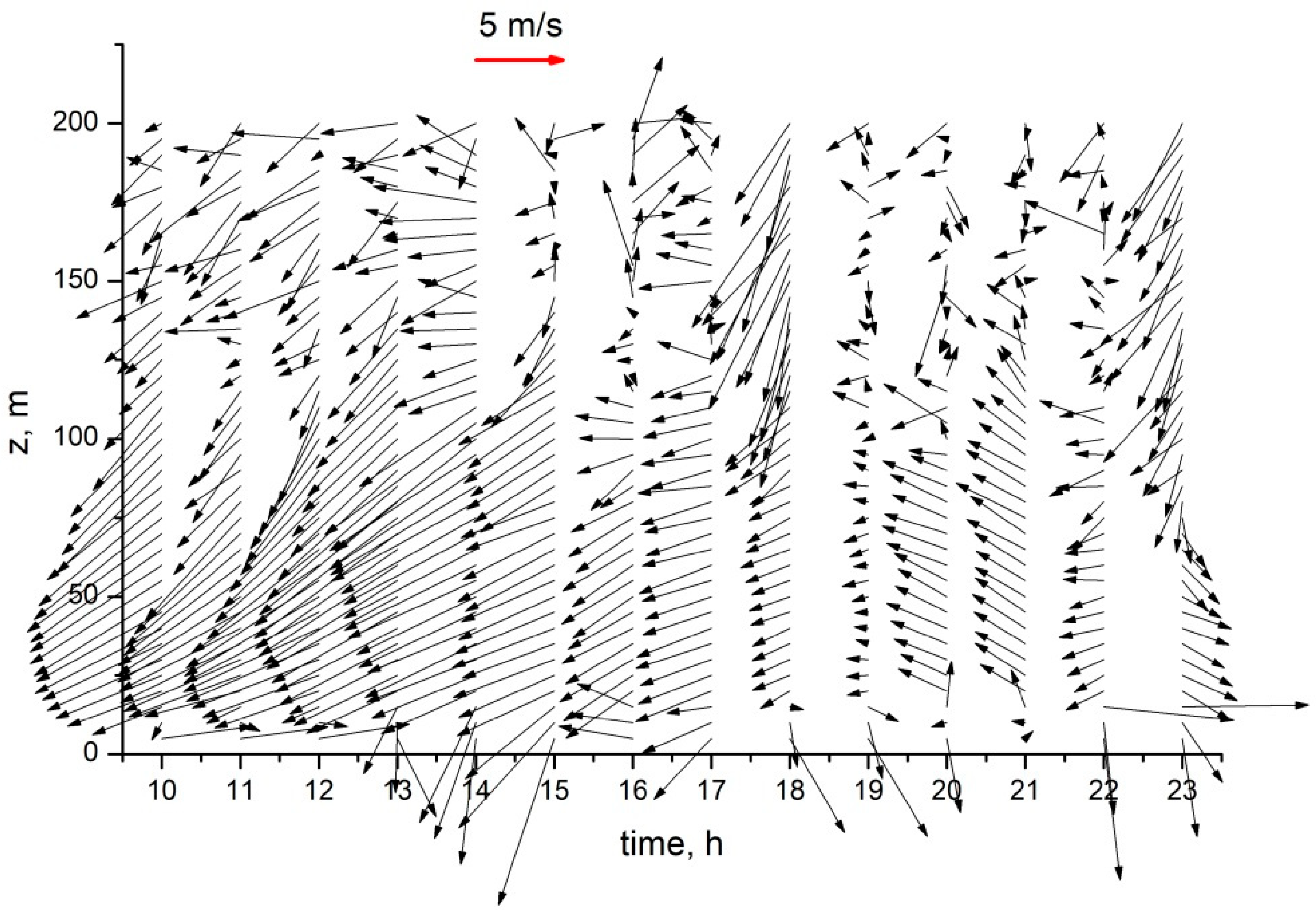
4.1. Diurnal Hourly Dynamics of the Wind Velocity Vector

Figure 1 shows the diurnal hourly dynamics of the wind velocity vector retrieved from minisodar measurements with 10-min averaging. The observations started at 10:00, local time, and finished at 24:00. Here, the length of the vector shows its magnitude, northern direction is upward, southern is downward, east is to the right, and west is to the left. It can be seen that irrespective of the observation time, the wind direction at altitudes up to 100 m undergoes no sharp changes with increasing altitude. At altitudes from 100 m to 200 m, the wind direction undergoes perturbations; moreover, if at 10:00 perturbations started from 150 m, at 14:00, they started already from 200 m. The lower horizon of the layer of enhanced turbulence descended from 16:00 till 17:00. As can be seen, from 10:00 till 17:00, the wind velocity vectors considerably exceeded their corresponding evening values (from 18:00 till 23:00), and a low-level jet was observed the maximum of which increased from 25 m at 10:00 to 75 m at 15:00.
Our analysis of the diurnal hourly dynamics of the x, y, and z wind vector components demonstrated that in the daytime, maximum values of the horizontal components were observed from 10:00 till 16:00–17:00. The minimal values of the horizontal components were observed late in the evening from 20:00 till 23:00. It is essential that at altitudes up to 50–100 m, the wind velocity vector did not experience sharp changes with increasing altitude and smoothly changed with the time of the day. At any time, maximal perturbations were observed at altitudes of 100–200 m; therefore, exactly this altitude range is most dangerous for UAV flights.
The results obtained demonstrated that at altitudes below 100 m, the direction of the wind velocity vector changed slightly depending on the time of the day. At altitudes of 100–200 m, the horizontal wind components increased at any time of the day, whereas the vertical component changed insignificantly. Visual analysis enables us to conclude that during time periods of maximal perturbations of the mean air motion (active turbulent air motion), the linear sizes of turbulent vortices are commensurable with the spatial resolution Δz = 5 m of the employed observation method. This is clearly seen for the observation period from 18:00 till 21:00.

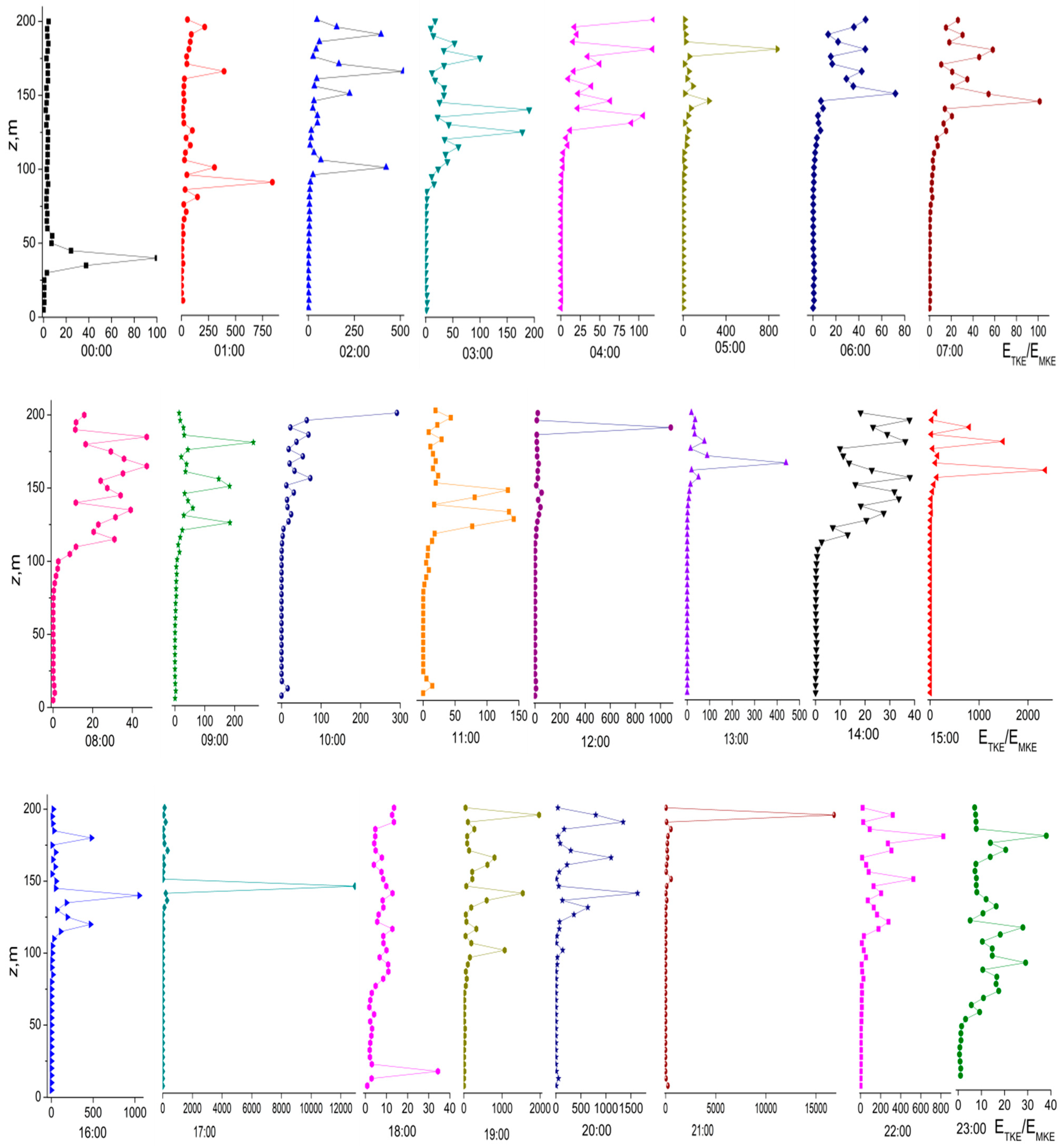
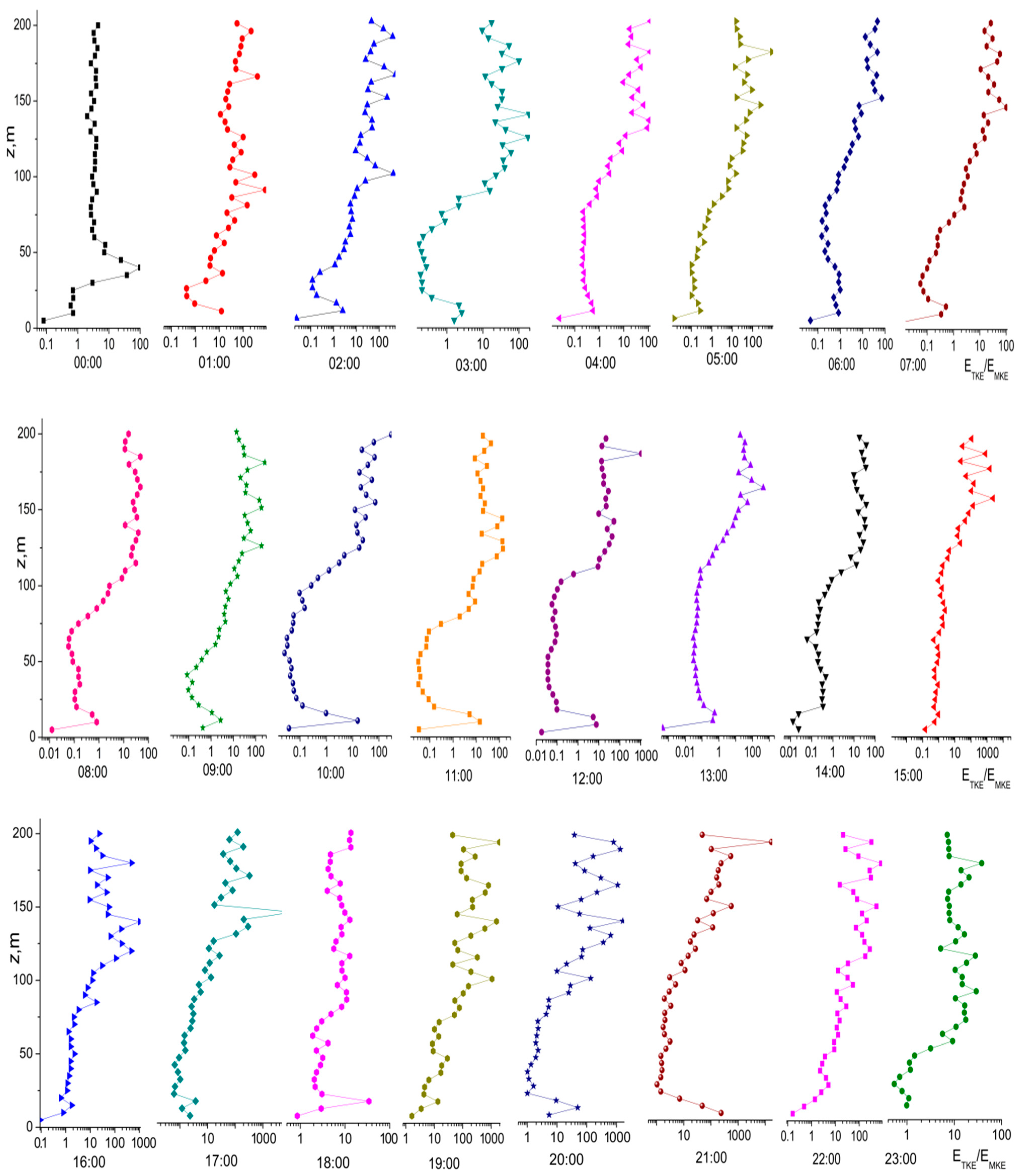
4.2. Diurnal Hourly Dynamics of Relative Contributions of the Mean and Turbulent Kinetic Energy Components

In this section, we analyze the spatiotemporal dynamics of the atmospheric kinetic energy E(z, t) retrieved from minisodar measurements. The components EMКE(zj, tk) and ETKE(zj, tk) in the jth strobe, j = 1, …, N, of the kth measurement series started at time tk, were calculated as follows [16]:
Е MKE ( z j , t k ) = 0.5 N 2 [ ( i = 1 N V x i j ( z j , t k ) ) 2 + ( i = 1 N V y i j ( z j , t k ) ) 2 + ( i = 1 N V z i j ( z j , t k ) ) 2 ] ,
E TKE ( z j , t k ) = 0.5 N 2 [ ( i = 1 N V x i j ( z j , t k ) V x ( z j , t k ) ) 2 + i = 1 N ( ( V y i j ( t k ) ) V y ( z j , t k ) ) 2 + i = 1 N ( ( V z i j ( t k ) ) V z ( z j , t k ) ) 2 ] ,
where V m i j ( z j , t k ) , m = x, y, z, are the wind velocity components measured with a minisodar in the jth range gate at altitude zj in the kth series of minisodar measurements started at time tk, and V m ( z j , t k ) are their 10-min averages. Of particular interest is the ratio δ(zj, tk) = ETKE(zj, tk)/EMКE(zj, tk) of the turbulent kinetic wind energy ETKE(zj, tk), determined by the variances of the wind velocity components, and the kinetic energy EMКE(zj, tk) of the mean motion of air masses, shown in Figure 2. This ratio characterizes situations in which the energy of mean (at δ(zj, tk) < 1) or turbulent (at δ(zj, tk) > 1) motions of air masses dominate. Moreover, its value quantitatively characterizes the dominating regime of air mass motion, which is especially important from the viewpoint of its effect on high-rise buildings and UAVs and on the wind energy potential of wind turbines.
Let us first analyze the time behavior of the ratio δ. Attention is drawn to the layers of enhanced turbulence, which was also indicated in [7]. From Figure 2, it can be seen that at 0:00, the turbulent kinetic energy was concentrated between z1 = 40 and z2 = 50 m, where it exceeded EMКE values by about 100 times. In this case, the turbulent layer thickness was 10 m. At other altitudes, ETКE was much lower than EMКE. At 01:00, two layers of enhanced turbulence were observed at 80 m (δ = 765), and 165 m (δ = 265). Below 80 m, turbulent energy dominated, but at higher and lower altitudes, the contribution of the turbulent kinetic energy becomes low. The situation changed with time. At 02:00, the lower boundary of the layer of enhanced turbulent energy increased to 100 m, and the upper stratified layer was recorded between 150–200 m, where δmax = 500. At 03:00, the stratified structure of the layer of enhanced turbulence was retained, and within this layer, δmax = 200. From 04:00 until 07:00, the lower horizon z1 of the enhanced turbulence layer rose to 130 m, and maximal δ values were observed at the layer bottom. By 04:00, δmax decreased to 100, but was already at the layer top. By 05:00, this tendency was retained, and δmax reached 800 at altitudes of 170–180 m, decreasing toward the layer bottom. From 06:00 to 07:00, the layer of enhanced turbulence was recorded between 150–200 m with δmax values equal to 80 and 100, respectively. At 08:00, δmax = 50, and z1 decreased down to 100 m. At higher altitudes, the δ value changed irregularly with altitude from 10 to 50. The thickness of the turbulent layer considerably increased (from z1 = 100 m to the maximum sounding altitude).
Thus, starting from midnight during night and early morning hours, the lower boundary of the layer of enhanced turbulence changed from 40–50 m at 0:00 to 150 m at 07:00 with nonmonotonic variations of δmax from 800 at 05:00 to 40 at 08:00.
In the morning (from 09:00 till 11:00), z1 slightly increased, and δmax decreased from 300 to 150. The situation changed at noon from 12:00 until 13:00. During this period, the thickness of the turbulent layer significantly decreased (down to 20–30 m), the height of its lower boundary z1 considerably increased, and the δmax value reached 1000 at 12:00. This thin layer of strong turbulence is dangerous for UAVs and high rise buildings due to very high δmax values. However, it is promising for wind energy applications. At 14:00, δmax decreased down to 40, and the thickness of the turbulent layer increased from 125 to 200 m. This was accompanied by nonmonotonic altitude variations of δ. In the afternoon, from 15:00 until 17:00, the thickness of the turbulent layer decreased to 10–20 m, but δmax sharply increased from 100 to 2000.
In the evening at 18:00, no layers of enhanced turbulence were recorded except those at altitudes between 15–20 m with δmax = 35. Here, the contribution of the mean kinetic energy dominated. The observation period from 19:00 till 21:00 was characterized by the maximum contribution of the turbulent kinetic energy. If at the beginning of this period the turbulence dominated starting from z1 = 100 m and non-monotonically changed with altitude, with increase in time, z1 increased, the turbulent layer thickness decreased to 20–15 m, but δmax reached 15,000 by the end of this period. In fact, a very thin turbulent layer was observed near the maximum sensing altitude that had a very high turbulent kinetic energy and hence is very dangerous for the UAVs and high-rise building and promising for wind energy applications. By midnight, from 22:00 till 23:00, the contribution of the kinetic energy decreased. The turbulent layer thickness decreased with increasing time with simultaneous decrease of δmax to 30–40 and decrease of z1.
Practically at any time, except around midnight (from 23:00 till 00:00), the contribution of the mean kinetic energy dominated at altitudes below 100 m; above this altitude, the relative contribution of the turbulent or mean kinetic energy depended on the time of the day and the sounding altitude.
It should be noted that at low δmax values (for example, at 08:00, 14:00, 18:00, and 23:00), the thickness of the layer of enhanced turbulence, as a rule, was large (from z1 = 50–100 m to 200 m). In this case, the turbulent kinetic flux energy density was not so large, but practically in the entire altitude range, the turbulent energy contribution prevailed.
On the other hand, at high δmax values (for example, at 05:00, 12:00, 17:00, and 21:00), the thickness of the layer of enhanced turbulence, as a rule, was small (10–15 m). This thin turbulent air layer transfers a large amount of turbulent kinetic energy and is dangerous for UAVs and high-rise buildings because of the unpredictable effect on them. Thus, based on the results obtained, we can conclude that the air kinetic energy in the lower 100 m layer weakly depends on the altitude z and increases with further increase in z. The diurnal behavior of radiative heating of the underlying surface causes the presence of minima and maxima of the wind kinetic energy whose occurrence depends on the meteorological conditions of observations.
The dependences of the ratio of the turbulent to the mean kinetic wind energy components δ(z) = ETKE(z)/EMKE(z) in linear coordinates visually characterize its behavior at altitudes z above 100 m and have allowed us to identify the layers of enhanced turbulence where the turbulent and mean kinetic wind energy components yield comparable contributions. At lower altitudes, where the contribution of the turbulent kinetic wind energy component is small and the ratio δ(z) lies in the range 0.01–10, the altitude dependence shown in Figure 3 on semi-logarithmic scale is more informative. In particular, four layers are clearly distinguished by the character of the altitude dependence of the ratio of the kinetic wind energy components established by us in [10]: the near-ground layer, the surface layer, the layer with linear increase of the kinetic wind energy components, and the transitive layer.
In the near-ground layer, at altitudes up to 25 m, attention is drawn to sharp changes of the ratio of the kinetic energy components; moreover, its maximum values were observed after midnight (01:00–02:00) and in the morning (09:00–12.00) and evening hours (18.00–22:00). This is explained by the influence of the underlying surface. At altitudes of 25-100 m, the ratio of the turbulent to mean kinetic energy weakly depended on the altitude, except the period after midnight (00:00–02:00). The character of the altitude dependence changed at night (03:00–04:00), in the afternoon (14:00–15:00), and late in the evening (21:00–22:00). In addition, at night and in the morning (00:00–14:00), δ(z) was in the range 0.01–100; in the evening, the span of its values increased to 0.01–1,000, and then from 23:00, it decreased again to 0.01–100.

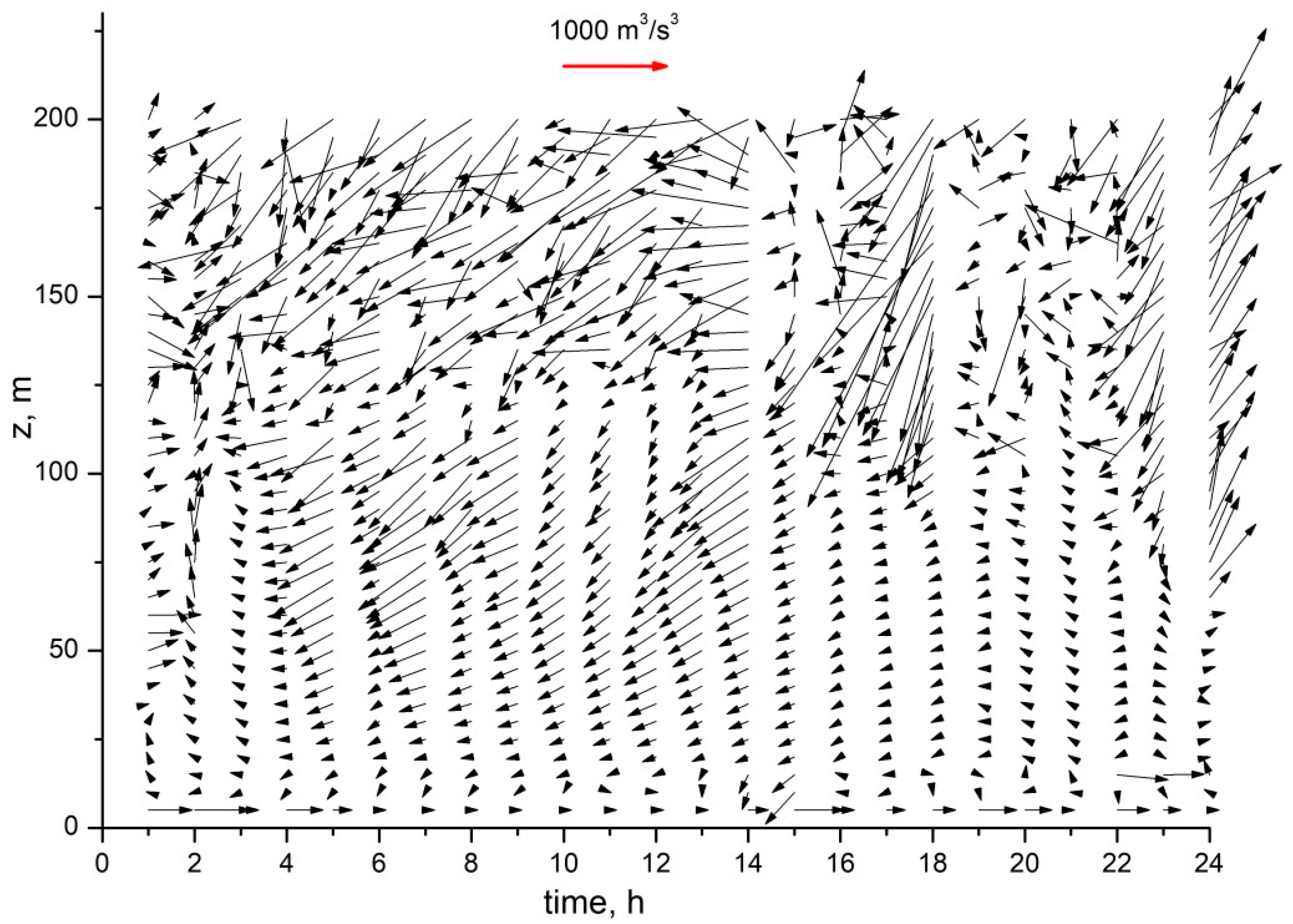
4.3. Diurnal Hourly Dynamics of the Total Kinetic Flux Energy Density Vector (the Umov Vector)

As already indicated in the introduction, the total wind kinetic energy flux density vector is used for an analysis and prediction of the dynamic wind effect. Figure 4 shows the diurnal hourly dynamics of the mean kinetic flux energy density vector j ( z , t ) obtained by postprocessing of minisodar measurements. The minisodar data were averaged over 10 min periods.
It should be underlined that this figure illustrates the total (mean and turbulent) kinetic energy transfer. It can be seen that it depends both on the time of the day and the sounding altitude. Three layers can clearly be distinguished in Figure 3: a near-surface layer at altitudes of 5–15 m, an intermediate layer at altitudes from 15 m to 150 m, and a layer of enhanced turbulence above. The irregular behavior of the kinetic energy flux vector in the near-surface layer is explained by the effect of the underlying surface. In the intermediate layer whose altitude zturb first increased from 25 m at 01:00 to 100 m at 03:00, the energy transfer in the north-western direction prevailed. From 05:00 till 15:00, the direction of energy transfer changed to south-western with simultaneous increase of zturb to 150 m. Then, from 15:00 till 18:00, the direction of energy transfer remained unchanged, but the lower boundary of the layer of enhanced turbulence zturb decreased to 100 m. From 19:00 until 22:00, the direction of energy transfer changed to north-western, and zturb decreased to 75 m.
From 23:00 until 24:00, the energy in the lower layer was transferred in the east-southern direction. Above this layer, in the layer of enhanced turbulence, the character of energy transfer changed radically, the kinetic energy flux density increased sharply, and the direction of energy transfer fluctuated due to a greater contribution of the turbulent kinetic energy component. The maximum kinetic energy flux densities were observed at 18:00, when the kinetic energy was predominantly transferred in the south-western direction. From Figure 3 it can be seen that the altitude range z > zturb and the time period from 06:00 till 18:00 are most dangerous for UAV flights [2]. The wind effect on high-rise buildings becomes most pronounced from 08:00 till 18:00, when the maximum values of the Umov vector were observed for z > zturb [3]. Meanwhile, these high values of the Umov vectors are promising for the wind energy potential of wind turbines directly proportional to the average kinetic energy flux density [4,5,17,18].

5. Conclusions

Based on post-processing of the data of minisodar measurement, a novel method of investigating the spatiotemporal dynamics of the kinetic energy flux density vector—the Umov vector—has been proposed and successfully realized. The diurnal hourly behavior of the vertical profiles of the mean and turbulent kinetic energy components and the wind velocity vector field in the lower 200-m layer of the atmosphere were analyzed together with the ratio of the turbulent to mean kinetic energy components. At night and morning hours (00:00–14:00), δ(z) was in the range 0.01–100; in the evening, the span of its values increased to 0.01–1000, and then since 23:00, it decreased again to 0.01–100. In the near-ground layer, at altitudes up to 25 m, attention is drawn to sharp changes of the ratio of the kinetic energy components; moreover, its maximum values were observed after midnight (01:00–02:00), and in the morning (09:00–12.00) and evening hours (18.00–22:00). This is explained by the influence of the underlying surface. At altitudes of 25–100 m, the ratio of the turbulent to the mean kinetic wind energy weakly depended on the altitude, except the period after midnight (00:00–02:00). The character of the altitude dependence changed at night (03:00–04:00), in the afternoon (14:00–15:00), and late in the evening (21:00–22:00). At altitudes below 100 m, the contribution of the turbulent kinetic wind energy component was small, and the ratio δ(z) was in the range 0.01–10.
The diurnal behavior of the Umov vector depended both on the time of the day and the sounding altitude. Three layers were clearly distinguished: the near-surface layer at altitudes of 5–15 m, the intermediate layer at altitudes from 15 m to 150 m, and the layer of enhanced turbulence above. The irregular behavior of the kinetic energy flux vector in the near-surface layer was explained by the effect of the underlying surface. In the intermediate layer whose altitude first increased from 25 m at 01:00 to 100 m at 03:00, the energy transfer in the north-western direction prevailed. From 05:00 until 15:00, the direction of energy transfer changed to south-western with simultaneous increase of the altitude of the intermediate layer to 150 m. Then, from 15:00 until 18:00, the direction of energy transfer remained unchanged, but the lower boundary of the layer of enhanced turbulence decreased to 100 m. From 19:00 until 22:00, the direction of energy transfer changed to north-western, and the lower boundary of the layer of enhanced turbulence decreased to 75 m. From 23:00 until 24:00, the energy in the lower layer was transferred in the east-southern direction. Above this layer, in the layer of enhanced turbulence, the character of energy transfer changed radically, the kinetic energy flux density increased sharply, and the direction of energy transfer fluctuated due to a greater contribution of the turbulent kinetic energy component. The maximum kinetic energy flux densities were observed at 18:00, when the kinetic energy was predominantly transferred in the south-western direction.
The spatiotemporal dynamics of the Umov vector can be used to elucidate time periods and altitude ranges of its maximal and minimal values as well as prevailing directions of total kinetic energy transfer, that is, to detect times and altitudes most and least favorable for flights of unmanned aerial vehicles, to estimate the effect of wind on high-rise buildings, and to predict the wind energy potential of wind turbines.

Author Contributions

Conceptualization, A.P., N.K. and L.S.; methodology, A.P., N.K. and L.S.; software, A.P., N.K. and L.S.; validation, A.P., N.K. and L.S.; formal analysis, A.P., N.K. and L.S.; investigation, A.P., N.K. and L.S.; resources, A.P., N.K. and L.S.; data curation, A.P., N.K. and L.S.; writing—original draft preparation, A.P., N.K. and L.S.; writing—review and editing, A.P., N.K. and L.S.; visualization, A.P., N.K. and L.S.; supervision, A.P., N.K. and L.S.; project administration, A.P., N.K. and L.S.; funding acquisition, A.P., N.K. and L.S. All authors have read and agreed to the published version of the manuscript.

Funding

This research was carried out with the financial support of the Russian Academy of Sciences within the framework of the State Assignment to the Institute of Monitoring of Climatic and Ecological Systems of the Siberian Branch of the Russian Academy of Sciences, Project No. 121031300155-8, and of the State Assignment to the V.E. Zuev Institute of Atmospheric Optics of the Siberian Branch of the Russian Academy of Sciences, Project No. 121031500227-0.

Institutional Review Board Statement

Not applicable.

Informed Consent Statement

Not applicable.

Data Availability Statement

Not applicable.

Conflicts of Interest

The authors declare no conflict of interest.

References

  1. Umov, N.A. The Equation of Motion for the Energy of a Body. Doctoral Thesis, Odessa University, Odessa, Ukraine, 1874. [Google Scholar]
  2. Fangwei, H.; Mohammad, J. Investigation approaches to quantify wind-induced load and response of tall buildings: A review. Sustain. Cities Soc. 2020, 62, 102376. [Google Scholar]
  3. Wang, B.H.; Wang, D.B.; Ali, Z.A.; Bai, T.T.; Wang, H. An overview of various kinds of wind effects on unmanned aerial vehicle. Meas. Control 2019, 52, 731–739. [Google Scholar] [CrossRef]
  4. Peña, A.; Hasager, C.B.; Badger, M.; Barthelmie, R.J.; Bingöl, F.; Cariou, J.-P.; Emeis, S.; Frandsen, S.T.; Harris, M.; Karagali, I.; et al. Remote Sensing for Wind Energy; DTU Wind Energy: Roskilde, Denmark, 2015; p. 260. [Google Scholar]
  5. Monzikova, A.K.; Kudryavtsev, V.N.; Larsen, E.S.; Chapron, B. Estimation of wind power potential of the Gulf of Finland. Proc. Russ. State Hydrometeorol. Univ. 2013, 30, 116–133. [Google Scholar]
  6. Banakh, V.A.; Smalikho, I.N. Coherent Doppler Wind Lidar; Publishing House of the Institute of Atmospheric Optics of the Siberian Branch of the Russian Academy of Sciences: Tomsk, Russia, 2013; p. 304. [Google Scholar]
  7. Bolbasova, L.A.; Shikhovtsev, A.Y.; Kopylov, E.A.; Selin, A.A.; Lukin, V.P.; Kovadlo, P.G. Daytime optical turbulence and wind speed distributions at the Baikal Astrophysical Observatory. Mon. Not. R. Astron. Soc. 2019, 482, 2619–2626. [Google Scholar] [CrossRef]
  8. Valldecabres, L.; Nygaard, N.G.; Vera-Tudela, L.; von Bremen, L.; Kühn, M. On the use of dual Doppler radar measurements for very short-term wind power forecasts. Remote Sens. 2018, 10, 1701. [Google Scholar] [CrossRef] [Green Version]
  9. Haggagy, M.A. A Sodar-Based Investigation of the Atmospheric Boundary Layer; Berichte des Meteorologischen Institutes des Universität Freiburg: Freiburg, Germay, 2003; p. 235. [Google Scholar]
  10. Potekaev, A.I.; Shamanaeva, L.G.; Kulagina, V.V. Spatiotemporal dynamics of the kinetic energy in the atmospheric boundary layer from minisodar measurements. Atmosphere 2021, 12, 421. [Google Scholar] [CrossRef]
  11. Shamanaeva, L.G.; Potekaev, A.I.; Krasnenko, N.P.; Kapegesheva, O.F. Dynamics of the kinetic energy in the atmospheric boundary layer from the results of minisodar measurements. Russ. Phys. J. 2018, 61, 2282–2287. [Google Scholar] [CrossRef]
  12. Tarasenkov, M.V.; Krasnenko, N.P.; Shamanaeva, L.G. Program for Constructing the Altitude-Temporal Distribution of Wind Velocity Components in the Lower Atmosphere from the Data of Acoustic Sounding; RF Certificate of State Registration of Computer Program, No. 2016619428; Rospatent: Moscow, Russia, 2016.
  13. Krasnenko, N.; Simakhin, V.; Shamanaeva, L.; Cherepanov, O. Robust nonparametric methods of statistical analysis of wind velocity components in acoustic sounding of the lower layer of the atmosphere. Symmetry 2019, 11, 961. [Google Scholar] [CrossRef] [Green Version]
  14. Doppler MiniSoDAR System: Operation and Maintenance Manual. Available online: https://home.chpc.utah.edu/~{}u0035056/5910_2010/Minisodarmanual.pdf (accessed on 30 December 2020).
  15. Yang, X. Atmospheric Acoustics; Walter de Gruyter GmbH: Berlin, Germany, 2016; p. 392. [Google Scholar]
  16. Underwood, K.H.; Shamanaeva, L.G. Turbulence characteristics from minisodar data. Russ. Phys. J. 2010, 53, 526–532. [Google Scholar] [CrossRef]
  17. Potekaev, A.I.; Shamanaeva, L.G.; Kulagina, V.V. Dynamics of the kinetic energy in the atmospheric boundary layer retrieved from the data of minisodar measurements. In Proceedings of the SPIE, 27th International Symposium on Atmospheric and Ocean Optics: Atmospheric Physics (in press), Moscow, Russia, 5–9 July 2021; p. 5. [Google Scholar]
  18. Sklyarov, Y.A. Development of Methods for Climatologic Estimation of the Wind Power Potential at Different Altitudes (on the Example of Southeastern Territory of Russia); Publishing House of Saratov State University: Saratov, Russia, 2012; p. 132. [Google Scholar]
Figure 1. Diurnal hourly dynamics of the wind velocity vector V ( z , t ) (northern direction—upwards, southern—downwards, east—to the right, and western—on the left).
Atmosphere 12 01347 g001
Figure 2. Diurnal hourly dynamics of the ratio of the turbulent to the mean kinetic wind energy components.
Atmosphere 12 01347 g002
Figure 3. Diurnal hourly dynamics of the ratio of the turbulent to the mean kinetic wind energy components on semi-logarithmic scale.
Atmosphere 12 01347 g003
Figure 4. Diurnal hourly dynamics of the kinetic energy flux density vector j ( z , t ) (northern direction—upwards, southern—downwards, east—to the right, and western—to the left). The magnitude of the vector is depicted by its length, and its direction coincides with that of the wind vector V ( z , t ) (see Figure 1).
Atmosphere 12 01347 g004
Publisher’s Note: MDPI stays neutral with regard to jurisdictional claims in published maps and institutional affiliations.

