
Modified Inverse Distance Weighting Interpolation for Particulate Matter Estimation and Mapping


Department of Future & Smart Construction Research, Korea Institute of Civil Engineering and Building Tech., Goyang-daero 283, Goyang-si 10223, Korea
*
Author to whom correspondence should be addressed.
Atmosphere 2022, 13(5), 846; https://0-doi-org.brum.beds.ac.uk/10.3390/atmos13050846
Submission received: 8 April 2022
/
Revised: 9 May 2022
/
Accepted: 19 May 2022
/
Published: 22 May 2022
(This article belongs to the Section Air Quality)
Abstract
:Various studies are currently underway on PM (Particulate Matter) monitoring in view of the importance of air quality in public health management. Spatial interpolation has been used to estimate PM concentrations due to that it can overcome the shortcomings of station-based PM monitoring and provide spatially continuous information. However, PM is affected by a combination of several factors, and interpolation that only considers the spatial relationship between monitoring stations is limited in ensuring accuracy. Additionally, relatively accurate results may be obtained in the case of interpolation by using external drifts, but the methods have a disadvantage in that they require additional data and preprocessing. This study proposes a modified IDW (Inverse Distance Weighting) that allows more accurate estimations of PM based on the sole use of measurements. The proposed method improves the accuracy of the PM estimation based on weight correction according to the importance of each known point. Use of the proposed method on PM10 and PM2.5 in the Seoul-Gyeonggi region in South Korea led to an improved accuracy compared with IDW, kriging, and linear triangular interpolation. In particular, the proposed method showed relatively high accuracy compared to conventional methods in the case of a relatively large PM estimation error.
1. Introduction
Urban air quality affects human life and health [1], and PM (Particulate Matter), one of the most important factors in determining air quality in industrialized countries, has adverse effects on physical and mental health [2,3,4]. PM causes physical health problems, including respiratory diseases, cardiovascular diseases, acute stroke, and fatalities [5,6,7,8,9,10,11,12], and is also known to adversely affect mental health, such as with depression and suicide [13].
As PM emerges as an important factor in public health management, real-time PM monitoring has become critical for PM control and reduction [14,15,16,17]. However, the high costs for installing and managing PM monitoring sensors and the limited detection range of these sensors make it difficult to analyze accurately the spatial variability of PM concentrations [18]. In other words, given that it is difficult to monitor sufficiently dense PM concentrations for an entire region of interest, local PM concentration information cannot be monitored continuously using only sensor measurements. In South Korea, additional PM stations have been installed during the past 20 years to manage public health through PM concentration monitoring. However, despite the continually increasing number of PM monitoring stations, each monitoring station covers an area which is far beyond its detection range. That is, one PM monitoring station is responsible for an area spanning approximately 167 km2 based on the entire country, or an area of 11 km2 based on the capital Seoul, wherein the monitoring stations have been constructed at the highest density. Therefore, it is challenging to observe the variation and spatial distribution of local PM concentrations only based on the monitoring station information, while an accurate prediction of PM concentrations is necessary for unmonitored locations to precisely estimate the public’s exposure to PM [17,19,20,21,22].
Spatial interpolation is one of the most reasonable and effective methods used to provide PM estimates for unknown points. It has been used in many previous studies to mitigate the limitations of monitoring networks [23,24,25]. Interpolation methods for PM estimation can be classified into (i) conventional methods using only relative location between points and (ii) methods with external drift. These two methods have opposite advantages and disadvantages. The conventional methods are relatively simple and easy to implement. However, they cannot reflect meteorological and geographic characteristics in PM estimation. Conversely, the interpolations with external drifts might estimate accurate PM concentration by using meteorological and geographic information, but the implementation is relatively limited because various additional data are required.
IDW (Inverse Distance Weighting) and kriging are representative conventional interpolation methods for PM estimation [18]. One of the most commonly used interpolation algorithms, IDW, is a deterministic interpolation method that uses the inverse distance between points for weighting. Various studies used IDW for PM trend evaluation [2,23,26] and long-term PM exposure analysis [7,8,9], as the process of IDW is fast and easy to use [12,27,28]. However, conventional IDW has limitations in local PM estimation, because it assumes a constant distance decay [27,29,30]. Kriging is a stochastic interpolation method that considers the distance between the measurement point and the prediction location, and the overall spatial arrangement between the points [6,23]. Many previous studies used kriging for macroscopic PM distribution mapping and evaluation [3,21,31,32,33]. The reason is that kriging can produce adequate results even with nonlinear data [14] and take into account variation bias. However, kriging requires care when modeling spatial correlation structures and needs relatively intensive computing [34].
The common disadvantage of conventional interpolation algorithms is that these methods are difficult to use for considering the effects of local or short-term characteristics of a target area in PM estimation [34,35]. This limitation of the conventional methods makes it difficult to perform accurate and stable interpolation for a local area [36] and also to distinguish the optimal algorithm [23,37,38]. In many previous studies, competitive evaluations have been performed to distinguish the best conventional method for PM estimation; however, the best interpolation method was varied in each different study. Some studies suggested that IDW is more suitable for PM estimation than the kriging-based method [6,39,40,41]. Conversely, in the other studies, the accuracy of the estimated PM concentration was the highest in the kriging method [1,20,25,42,43,44].
Interpolation methods with external drifts can reduce the limitation of the conventional method and improve the accuracy of PM estimation by considering the geographic and meteorological characteristics of the target area in PM estimation. In previous studies, the PM interpolation methods with external drifts have shown more accurate results than the conventional methods by using data such as wind, temperature, humidity, visibility, precipitation, transportation network, land use, DEM (Digital Elevation Model), and population [5,14,19,35,45]. However, interpolations with external drifts have the following disadvantages. First, the interpolations with external drifts are more difficult to implement and limited to apply than the conventional methods. The methods with external drifts require various data and corresponding handling processes in each data. Some algorithms use a dozen kinds of data in PM interpolation and occasionally require big data such as DEM, satellite, and aerial imagery [35]. Therefore, additional processes and intensive computing are entailed in PM interpolation with external drifts. Furthermore, the optimal method is unclear because essential drifts vary depending on the characteristics of each target area [18,38,46].
The objective of this study is to suggest a PM interpolation method that solves the limitations of the previous interpolation methods. More specifically, this study aims to develop a PM interpolation method that reflects the comprehensive characteristics of the target area without external drifts. The modified IDW proposed in this study adopts weight adjustment to reflect the effects of characteristics of the target area. The weight adjustment of the proposed method is conducted by means of the correction coefficients, which are derived empirically using only the observations. Therefore, the proposed method requires no variable input in addition to the PM observations and is easier to implement compared with the interpolation methods with external drifts. Additionally, the proposed method may provide accurate estimations compared with the conventional methods that cannot reflect geographic and atmospheric characteristics.
This paper describes the research contents in the following order. First, Section 2.1 describes the PM observations used in the experiment and the preprocessing of the observed values. Section 2.2 explains the conventional interpolation methods (IDW, kriging, linear triangular interpolation) used in the cross validation and a proposed modified IDW. Subsequently, Section 3 describes the comparative analysis of the interpolation results for the subject area. Finally, Section 4 draws conclusions on the findings of this research and looks ahead to upcoming work.
2. Materials and Methods
2.1. Study Area and Preprocessing for Experimental Data
The subject area of this study is the Seoul and Gyeonggi-do regions in Korea. Seoul, the capital of Korea, and the nearby Gyeonggi-do region, are important areas for estimating PM concentrations at the local level because there are densely populated cities with more than 20 million people. Additionally, the study area is suitable for determining the performance of spatial interpolation, as it encompasses various factors that can affect the local distribution characteristics of air quality, such as high-rise buildings, roads, vehicles, and topographical changes.
In this study, the hourly PM2.5 and PM10 concentration data measured at a total of 100 national monitoring stations for 1 year and 6 months (1 January 2020 to 31 May 2021) were used. The PM concentration data were acquired through sensors that employ a β-ray absorption method installed in each monitoring station (Figure 1b). In the subject area of the study, a PM monitoring network, which consisted of a total of 130 national monitoring stations, was operated. While monitoring station data with measurements omitted for more than 100 days during the target period of 1 year and 6 months were excluded from the experiment, PM observation data measured at a total of 100 monitoring stations were used. Figure 1b shows the monitoring stations (locations of PM concentration measurement) used in this study. Among all monitoring stations, observations at 70 monitoring stations (blue dots in Figure 1) were used as reference data, whereas observations at the remaining 30 monitoring stations (red dots in Figure 1) were used for accuracy validation. The average distance from one reference station to the nearest four reference stations is 7.75 km, and the average distance from one validation station to the nearest four reference stations is 5.45 km (Table 1).
In this study, outliers in the PM concentrations were eliminated by preprocessing the data prior to interpolation. Although the hourly PM concentrations used in the study had been passed through a simple screening process depending on whether the sensors were operating normally, and based on the rate of change in the measured values, some outliers still remained. Therefore, the data in this study were preprocessed for data refinement based on (i) a comparison between PM10 and PM2.5 concentrations and (ii) local outlier detection.
In the first step of data refinement, when the PM10 concentration is less than the PM2.5 concentration, both the PM2.5 and PM10 measurements are eliminated. PM2.5 and PM10 indicate Particulate Matter which is smaller than 2.5 μm and 10 μm, respectively, and PM10 includes PM2.5. Therefore, when the PM10 concentration is less than PM2.5, either of these two levels can be considered an erroneous measurement.
In the second step of data refinement, considerably high or low PM concentrations are excluded from the PM concentrations measured continuously at a single location. In this study, “an element that is greater than three scaled media development (MAD)” was regarded as an outlier among the PM concentration values observed for six consecutive hours. Herein, the scaled MAD is calculated based on Equations (1) and (2), where M is an observed PM concentration, k is the scaling factor, median is the median function, and erfcinv is the inverse comprehensive error function.
2.2. Spatial Interpolation Method for PM Estimation
This study proposes a modified IDW method that introduces a distance weighting correction coefficient to conventional IDW to improve the accuracy of PM2.5 and PM10 interpolation. In this section, the proposed modified IDW is described in detail. Prior to the description of the proposed method, the conventional interpolation methods used for cross validation are described briefly, including IDW, kriging, and linear triangular.
2.2.1. Conventional Spatial Interpolation Method for Cross Validation
The first approach used in the cross validation of the proposed interpolation method was IDW. IDW interpolation is based on the assumption that the values at points close to each other are more similar than at points which are further away. That is, IDW is a deterministic interpolation method that assumes a constant spatial distance–attenuation relationship [27,47]. Accordingly, in IDW, a relatively greater weight is assigned to a known point located close to unknown points, and a relatively smaller weight is given to a known point located far away. This concept of IDW is expressed as shown in Equations (3) and (4), where is the estimated value used for the target interpolation location, n is the number of reference (measured) values near the target location, is the weight of the ith reference (measured value), is the distance between the target location and the ith point, and α is a constant power used to adjust the diminishing strength in relationship with increasing distance. In this study, α was set to the value of two based on previous studies. Previous studies on PM interpolation [1,8,48] suggested an α value of two as optimal for PM.
The second conventional interpolation method used in the comparison and validation of the proposed interpolation method is ordinary kriging (OK). The kriging method determines a value based on statistical analysis of the neighboring measured values. In other words, kriging determines the weighting using spatial autocorrelation rather than the inverse distance between data [25]. Kriging is classified into ordinary, simple, universal kriging, etc., depending on the stochastic properties of the random field and the variable degrees of stationarity assumed [40]. Among the different kriging methods, ordinary kriging (OK) was used in this study for the following reasons. OK is one of the most commonly used kriging methods [14] and has been applied for PM interpolation in several previous studies [15,16,25,27,33,36,44,45]. Particularly, a few previous studies [25,36,44] suggested that OK was the most suitable approach among the kriging methods for PM interpolation in Korea. Son et al. [25] identified OK to be the most suitable for PM interpolation according to the cross validation of ordinary, simple, and universal kriging. Kim et al. [44] determined that OK with the Gaussian semivariogram model was the most suitable kriging approach for PM interpolation in Korea. Accordingly, Gaussian model-based OK was applied in this study for the cross validation of the proposed method.
The last interpolation method used for cross validation is linear triangular interpolation. This method uses the nearest three known points to interpolate for the unknown point. That is, the linear triangular method is based on the assumption that x, y, and Z (measurements) of the unknown point should be placed over a three-dimensional (3D) triangular plane with the nearest three known points (, , ) as vertices. This method has the advantage of processing efficiently large-scale data while providing simple calculations and yielding relatively accurate estimates [49]. As an interpolation method that is easy to implement with a very short processing time, the linear triangular method was selected as a method for cross validation in this study.
2.2.2. Proposed Modified IDW Interpolation
The modified IDW proposed in this study does not determine which and how external drifts affect the PM distribution, but only empirically estimates the total amount of the influence of various external drifts on the PM distribution to correct the distance-based weights. In the proposed method, when the observation does not follow the distribution tendency of the other, the observation is considered to be strongly influenced by external drifts. Therefore, the weight of this observation is adjusted to be higher, because it reflects the characteristics of the local area better than other observations. This approach contributes to efficient and accurate interpolation because characteristics of the target area can be reflected comprehensively without external drifts.
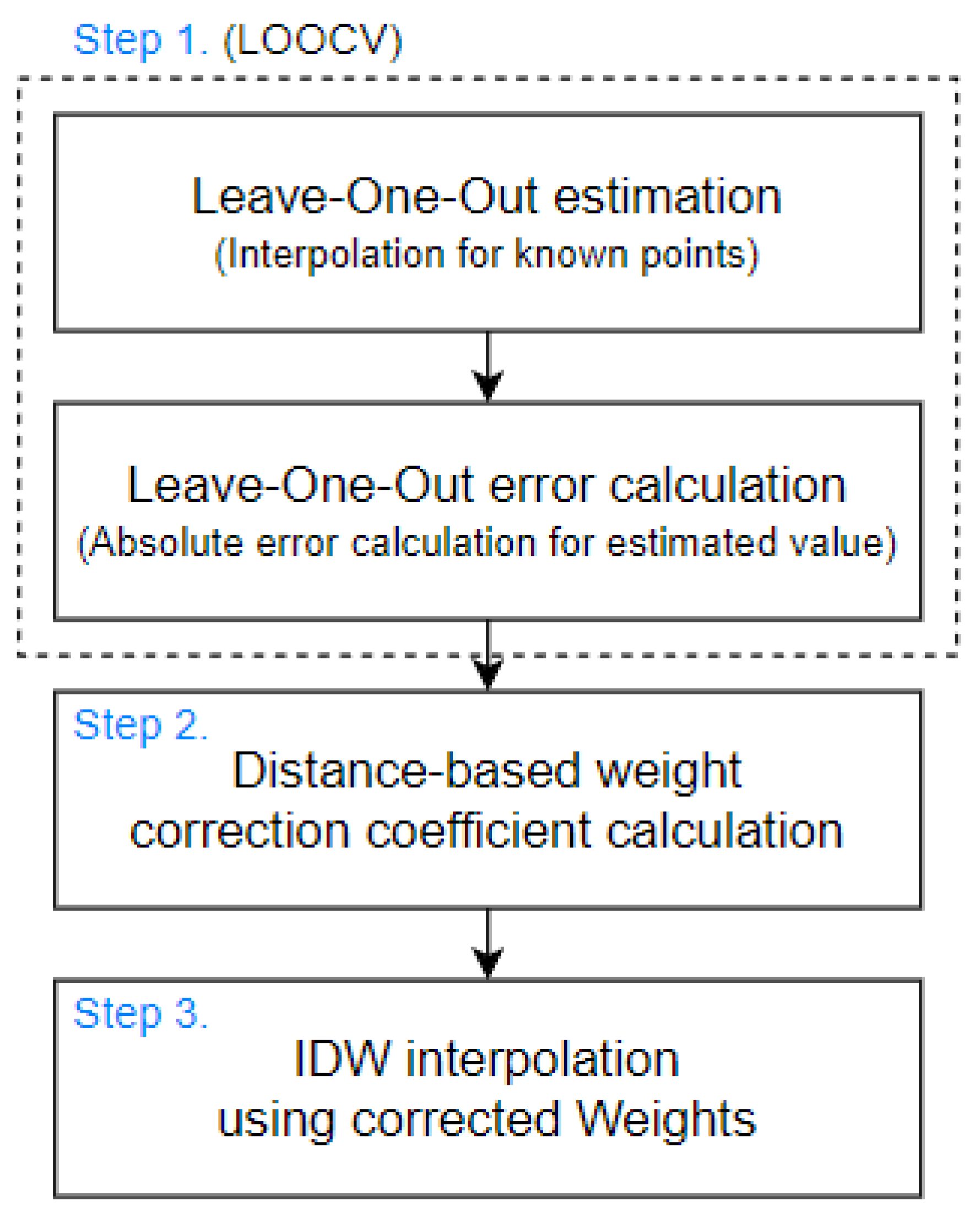
In the proposed method, it is believed that as the estimation accuracy based on the use of neighboring (known) points decreases, the observation at the corresponding point for the estimation of nearby unknown points becomes more important. Conversely, when the estimated PM concentration is very similar to the actual measured value, the PM in the nearby area can be estimated with sufficiently high accuracy using the neighboring known points, and the corresponding point becomes less important. In other words, in the proposed method, known points with relatively low estimation accuracy are considered to have been locally affected by external drifts that are distinctive from other known points, and are thought to be more important for estimating nearby unknown points, thus resulting in a greater distance weight. Figure 2 shows the modified IDW process (Figure 2).
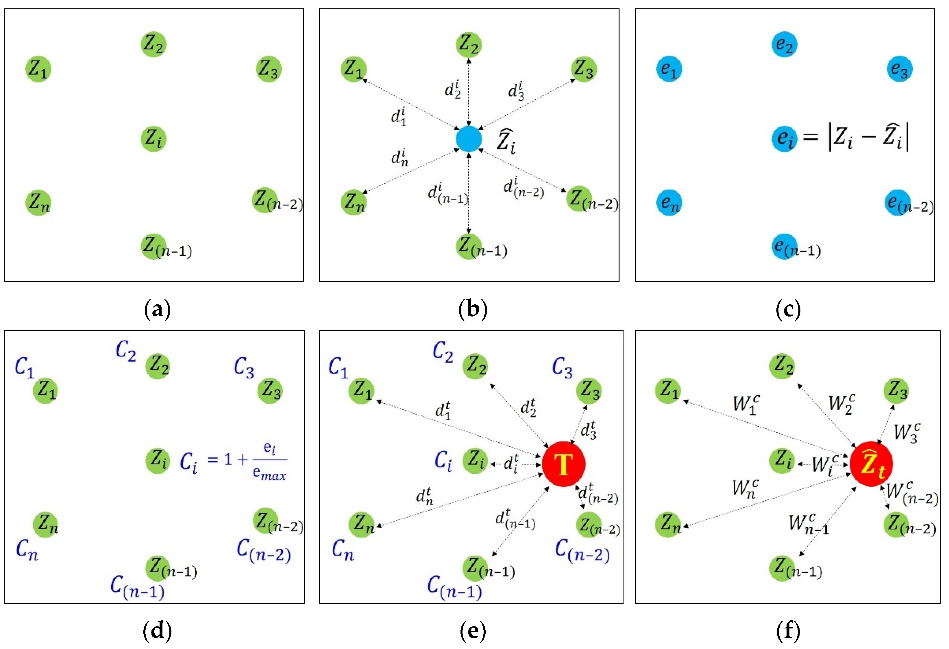
In the first step, the interpolation accuracy for each known point is calculated based on the Leave-One-Out Cross Validation (LOOCV). Given n measurements (Z1, Z2, …, Zn−1, Zn) for n points (green circles in Figure 3a), an estimate ( for the ith point (blue circle in Figure 3b) is calculated based on IDW interpolation using the neighboring observations (Figure 3b). That is, the estimated value for each known point is derived by performing Leave-One-Out interpolation. Subsequently, the absolute error, ei, of LOOCV is calculated using the observed value, Zi, at the ith point. This first step is repeatedly performed until the absolute error of LOOCV is calculated at all known points (Figure 3c).
In the second step, the weight correction coefficient for each known point is calculated by normalizing the absolute error of LOOCV. The normalized absolute error, which is the weight correction coefficient, is calculated by Equation (5). In Equation (5), ci is the weight correction coefficient for the ith known point, and emax is the maximum absolute error of LOOCV. The weight correction coefficient calculated based on this normalization has a value in the range from one to two. That is, the weight correction coefficient is equal to one for the point at which the absolute error of LOOCV is zero, whereas the correction coefficient is equal to two for the point which exhibits the maximum error. This process is repeated until the correction coefficients of all known points are determined (Figure 3d).
In the third step, the weight is adjusted using the correction coefficient, and IDW interpolation is performed. When there is an unknown point T (red circle), as shown in Figure 3e, the interpolation for the corresponding point is calculated based on Equations (6) and (7) (Figure 3f), where is the estimated value of the unknown point calculated based on interpolation, n is the number of neighboring known points, is the corrected weight for the ith known point, and is the distance between the ith known point and point T. In Equation (7), when there is a known point with a correction coefficient of one, the inverse distance of the corresponding point is reflected in the weight calculation as it is. Conversely, in the case of a known point with a correction coefficient of two (maximum error), the inverse distance of the corresponding point is reflected in the weight calculation as a double value. In other words, the known point with the low accuracy associated with LOOCV is considered to be a point reflecting local specificity and is considered important in the interpolation process.
The main difference between the proposed method and conventional IDW is that the proposed method does not depend solely on the distance between points. In the conventional IDW, once the known and unknown points are determined, the distance between the points is identified, and the distance weighting does not change by default. Conversely, given that the weight of the modified IDW is adjusted according to the significance of the observed value at a specific point in time, the characteristics of the observed value at that point are considered in interpolation.
3. Results and Discussion
The modified IDW proposed in this study is comparatively evaluated through estimations for 30 points using the PM10 and PM2.5 data observed at 70 stations in Seoul-Gyeonggi-do, Korea. The methods used for estimating the PM concentration included the proposed modified IDW, IDW, kriging, and linear triangular interpolation. The performance of the method was evaluated with the RMSE (Root Mean Square Error) and MAPE (Mean Absolute Percentage Error) of estimated PM concentrations.
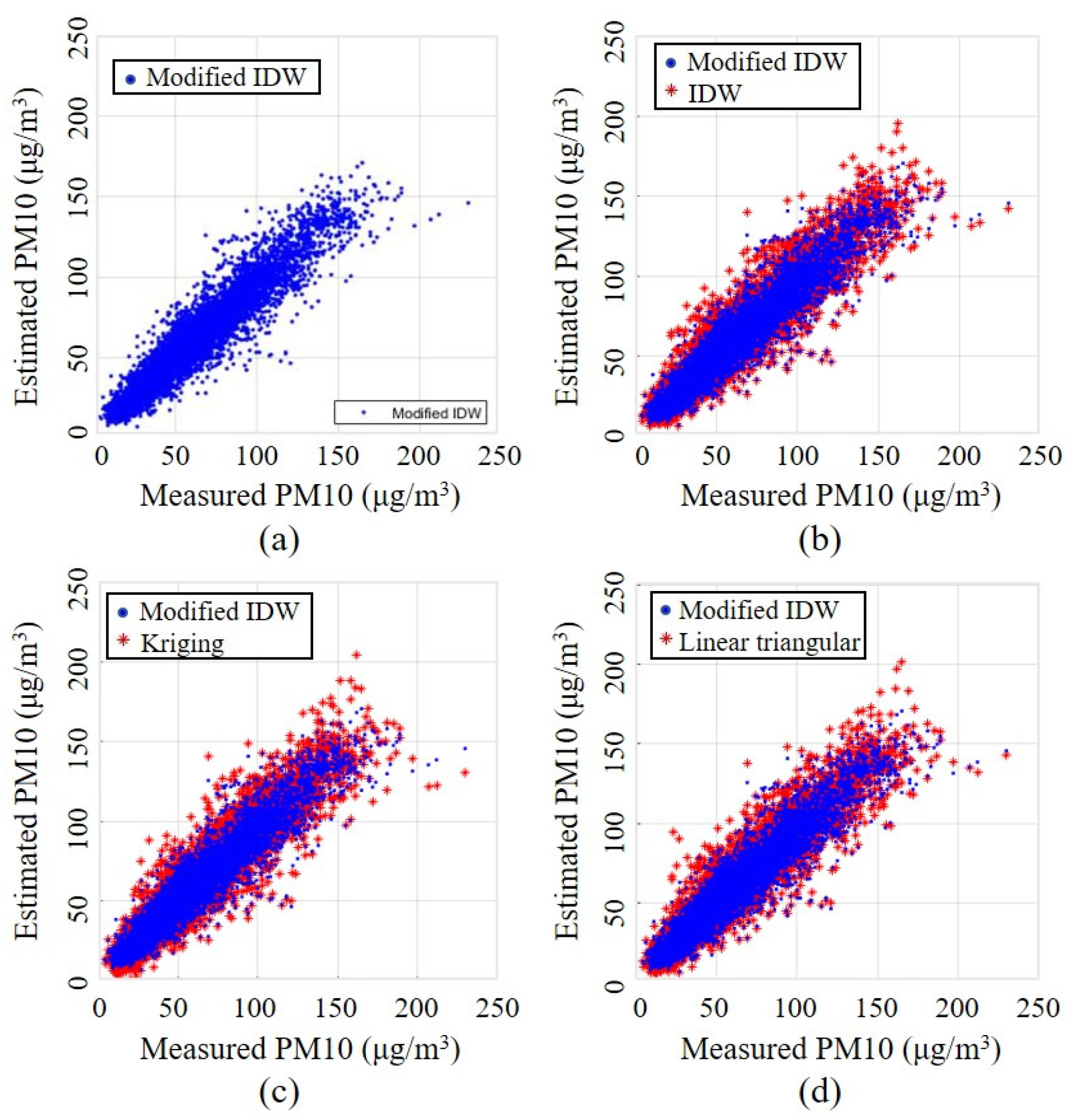
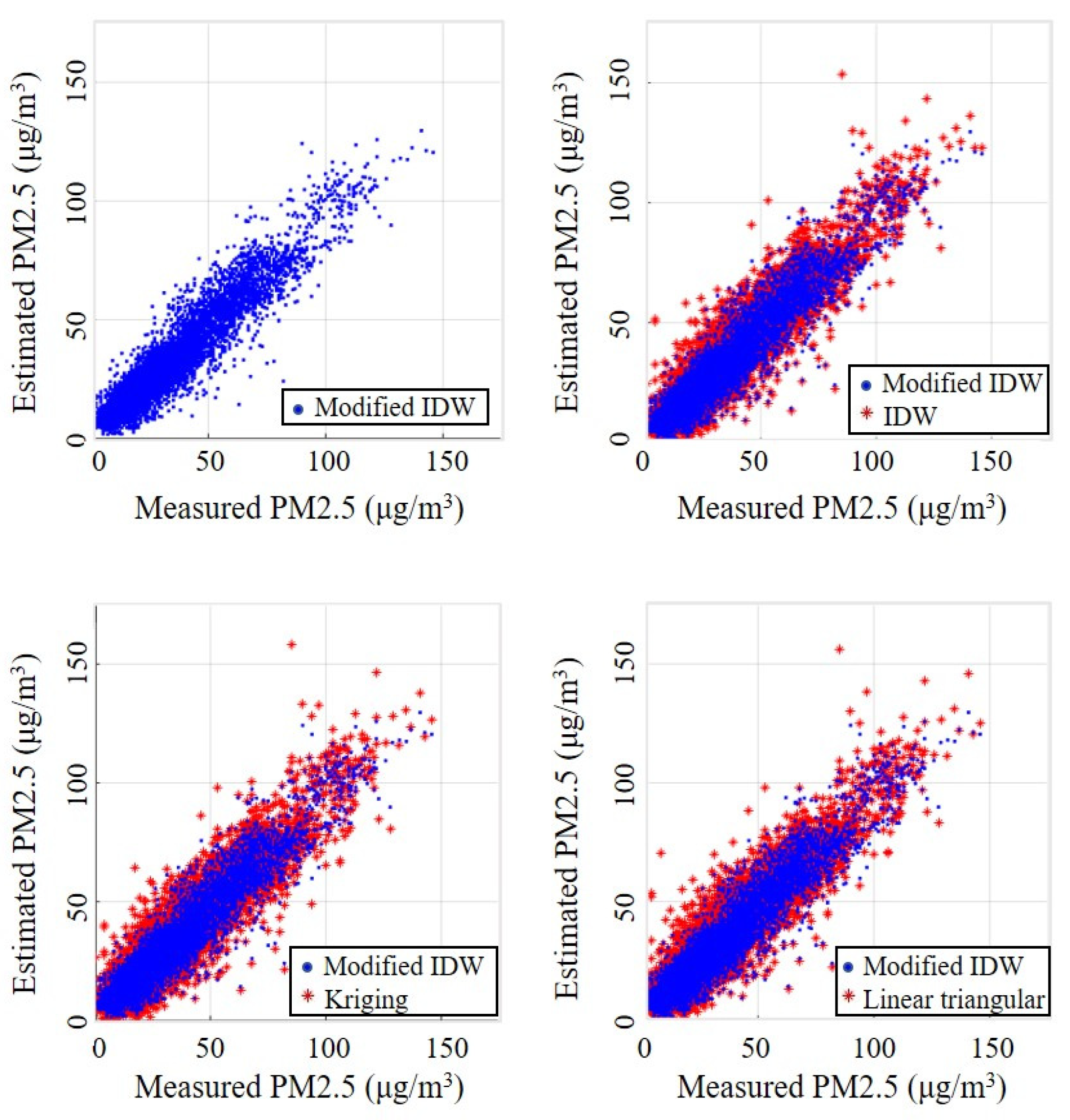
The modified IDW showed better performance than conventional methods for both the PM10 and PM2.5 interpolation. Table 2 shows RMSE and MAPE of interpolations for PM10 and PM2.5. The results of modified IDW achieve the lowest RMSE and MAPE. The accuracy of the interpolation methods in terms of RMSE and MAPE decreased in the order of the modified IDW, IDW, linear triangular, and kriging. Figure 4 and Figure 5 show the comparisons of the PM10 and PM2.5 concentrations estimated with each interpolation method and the observed values. The blue dots in the figures indicate the results of the proposed modified IDW, and the red asterisks indicate the results obtained from the conventional methods. Figure 4 and Figure 5 show that the proposed interpolation method estimates PM10 and PM2.5 more accurately compared with the other methods
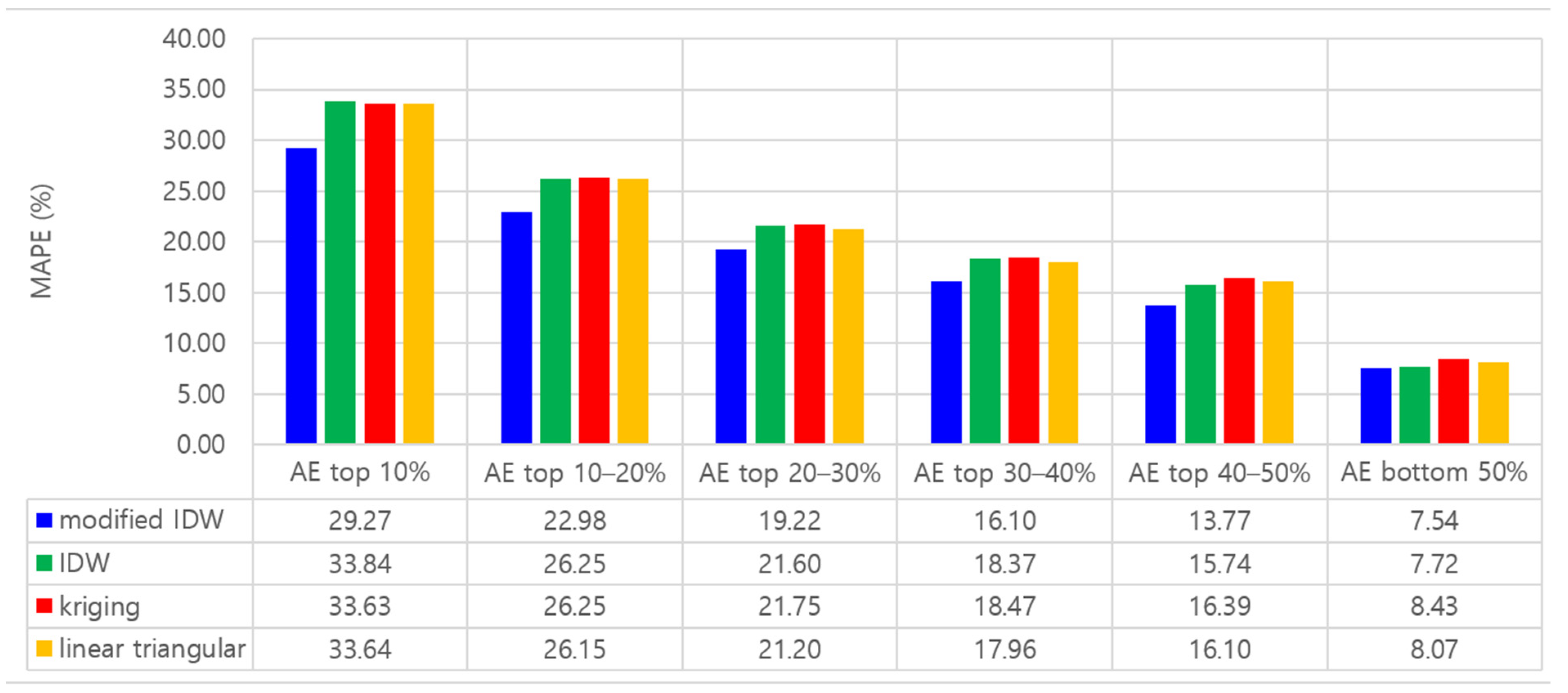
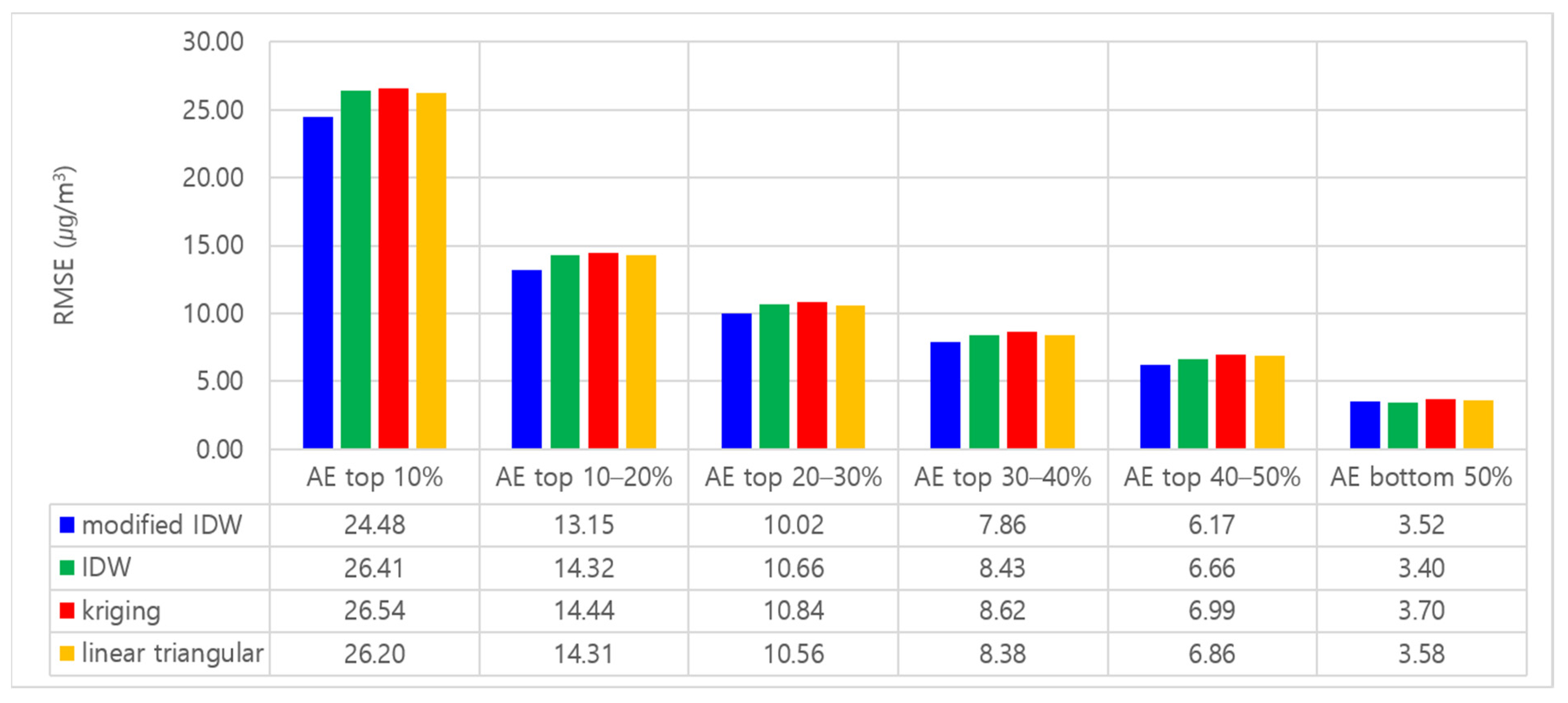
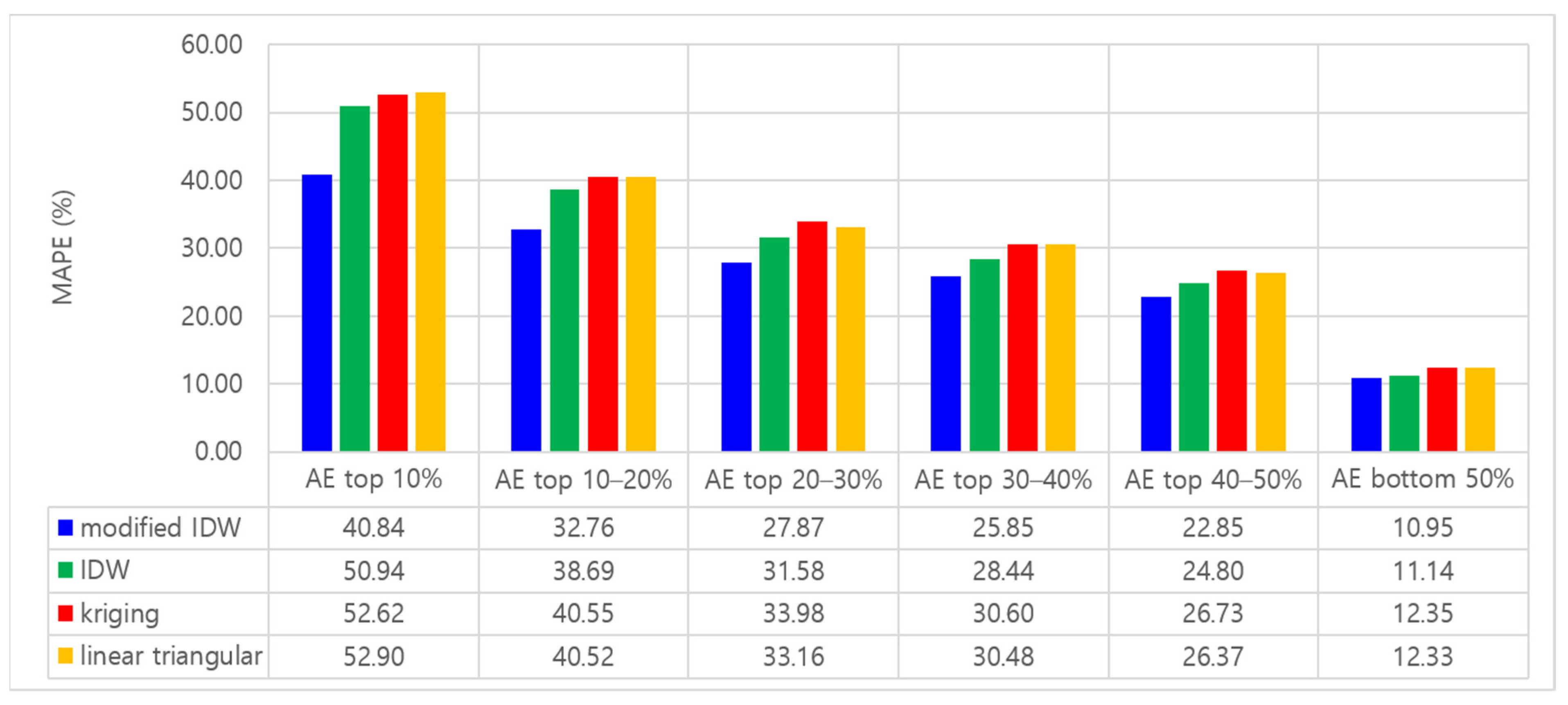
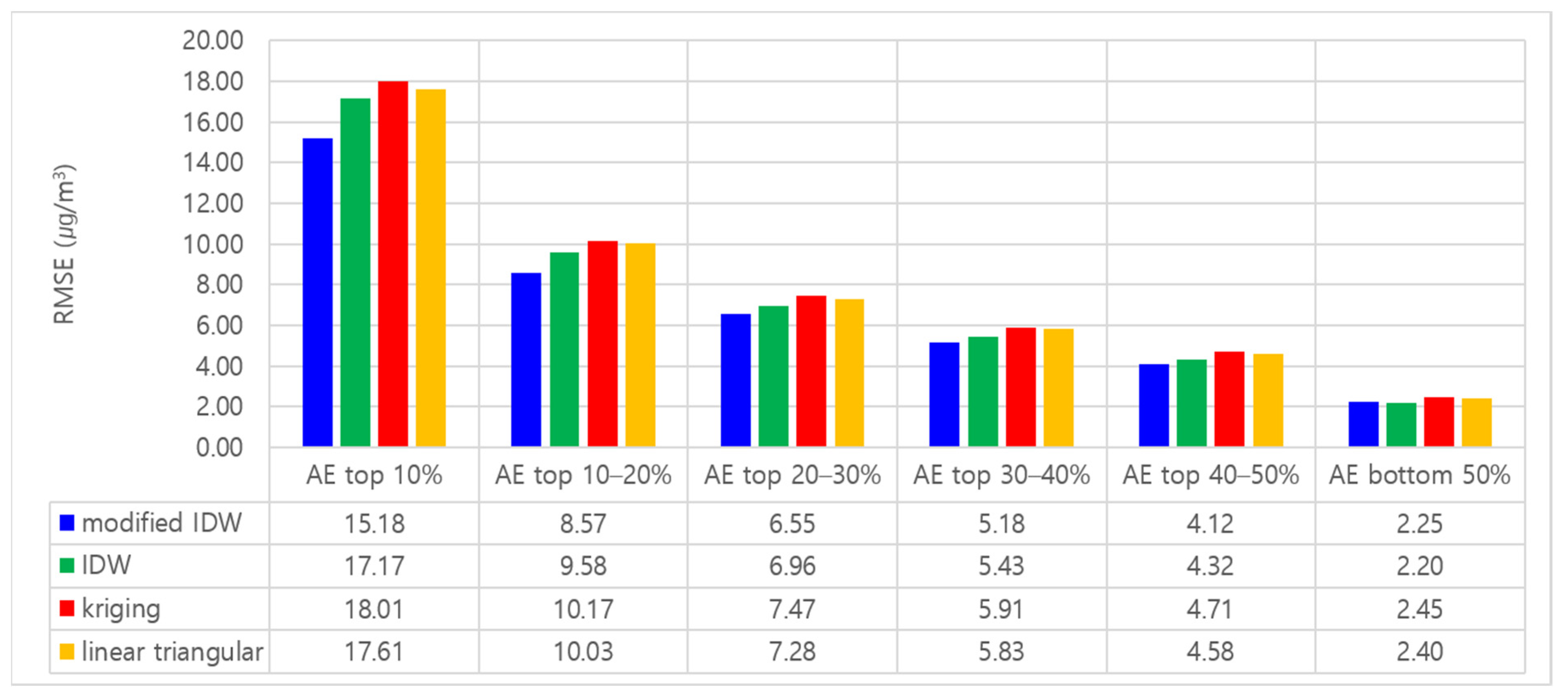
In this study, in order to more clearly confirm the performance improvement of the proposed method that came from the reflection of the local specificity that cannot be explained by the relative positional relationship, the results of interpolations were compared according to the AE (absolute error) level of the PM estimation. To this end, PM estimations were classified into six groups according to AE levels: AE top 10%, 10–20%, 20–30%, 30–40%, 40–50%, and bottom 50%.
The performance of modified IDW was generally better than the conventional methods for all AE groups. In particular, for groups of higher AE, the accuracy differences between the proposed and the conventional methods were increased. Figure 6 and Figure 7 show the MAPE and RMSE of the PM10 interpolation for each AE group. These figures confirm the MAPE and RMSE of PM10 estimations using the proposed method were generally lower than the conventional methods regardless of the AE groups. Additionally, the larger the value of AE, the relatively higher the accuracy is in the case of the modified IDW compared with those of the other algorithms. That is, for the AE top 10% group, the MAPE and RMSE values of the proposed method were 4.36–4.57% and 1.72–1.93 μg/m3 lower than the other methods. Figure 8 and Figure 9 show the MAPE and RMSE of the PM2.5 interpolation for each AE group. The accuracy of the PM2.5 estimation for the AE groups exhibited a similar tendency to that of PM10. That is, the proposed method achieved the lowest MAPE and RMSE values. Furthermore, as the AE increased, the differences between the error of the proposed and other methods increased. In the case of PM2.5, the MAPE and RMSE values of the modified IDW in the AE top 10% group were 10.10–12.06% and 1.99–2.83 μg/m3 lower, respectively, than those of the other methods.
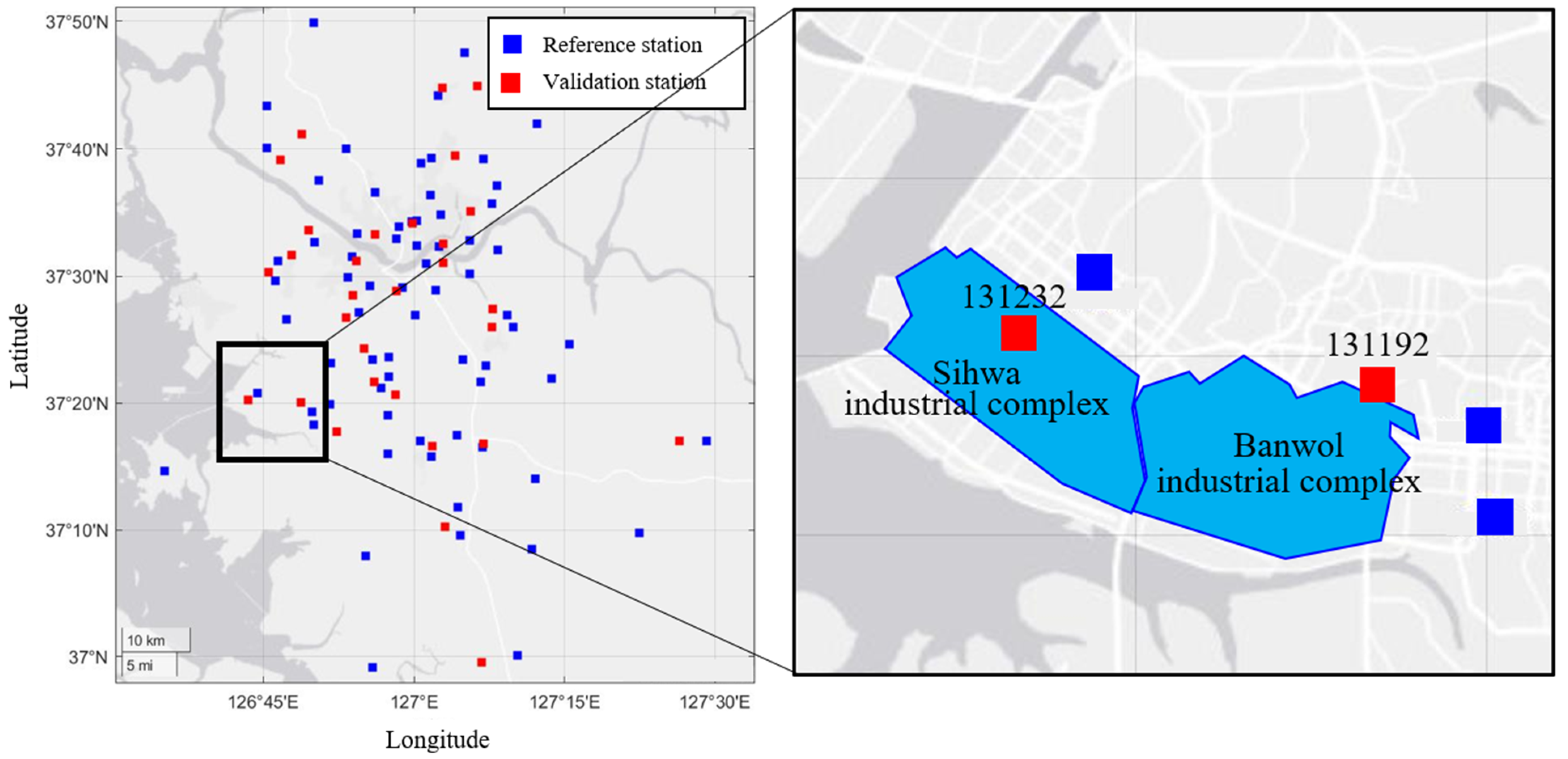
In this study, the error is confirmed for each validation station to evaluate the proposed method precisely (Table 3). Among all the validation stations, those that exhibited the highest error based on RMSE were the stations 131192 (20.98 μg/m3) and 131232 (15.10 μg/m3). The reason that estimations of stations 131192 and 131232 show relatively lower accuracy is as follows. Most spatial interpolation methods, including the proposed method, determine the estimate within the maximum and minimum range of observations. Therefore, without observations for a point showing a significantly different PM concentration, the accuracy of PM estimations can be decreased, where stations 131192 and 131232 are located near the industrial areas (Sihwa and Banwol industrial complex), and the reference stations around them are located in residential areas (Figure 10), and they show consistently higher concentrations of PM10 and PM2.5, respectively. At the time of observation (the year 2020), monthly mean PM10 concentrations of station 131192 were 19–25 μg/m3 higher, and monthly mean PM2.5 concentrations of station 131232 were up to 12 μg/m3 higher than the surrounding reference stations. On the other hand, the PM2.5 concentration of station 131192 and the PM10 concentration of station 131232 did not show a significant difference from those of neighboring reference stations. This tendency of PM distribution explains the reason for the highest errors in the two stations.
4. Conclusions
The aim of this study was to propose an interpolation method to accurately and efficiently estimate PM10 and PM2.5. To this end, this study proposed a modified IDW interpolation method. The proposed method does not require external drifts and has the advantage of performing accurate PM interpolation through IDW weight correction.
In the proposed interpolation method, the inverse distance weight is adjusted using the correction coefficient derived from empirical evaluations for PM observations. The proposed method adjusts the weight of the known point higher, as the accuracy of the corresponding LOOCV is lower. It is based on the assumption that the estimation and observation values show the distinct difference for a point showing PM distribution that is differentiated from the neighbors according to the characteristics of the local area.
In this study, the performance of modified IDW was comparatively evaluated with conventional methods. The proposed method shows better performance in both PM10 and PM2.5 estimations compared with conventional IDW, kriging, and linear triangular interpolation. The MAPE of PM10 and 2.5 estimations using the proposed method were 1.53–1.96% and 2.52–4.13% lower, respectively, than conventional methods. In particular, the performance improvement of the proposed method was confirmed when the conventional methods showed a large error. In the top 10% of the estimation error, the MAPE of PM10 and 2.5 using the proposed method were 4.36–4.57% and 10.10–12.06% lower, respectively, than the other methods. However, the proposed method shows the limitation that the estimated value is determined within the range of the minimum and maximum values of observations, as with many previous spatial interpolation methods. Therefore, when there is no observation for a point showing a significantly higher (or lower) PM concentration than the neighboring area, the accuracy of PM estimations can be decreased.
This study will contribute to air quality monitoring in the following ways. The modified IDW proposed in this study is significant in that it can support efficient spatial-continuous PM monitoring. Next, we believe that the proposed method can be adopted for various substances related to air quality. In future studies, we plan to advance further the proposed method to take into account both spatial and temporal differences. We also intend to develop air quality monitoring and mapping technologies by applying the proposed interpolation method and imagery data.
Author Contributions
Conceptualization, K.C. (Kanghyeok Choi); methodology, K.C. (Kanghyeok Choi); software, K.C. (Kanghyeok Choi); validation, K.C. (Kanghyeok Choi) and K.C. (Kyusoo Chong); formal analysis, K.C. (Kanghyeok Choi) and K.C. (Kyusoo Chong); investigation, K.C. (Kanghyeok Choi); resources, K.C. (Kyusoo Chong); data curation, K.C. (Kanghyeok Choi); writing—original draft preparation, K.C. (Kanghyeok Choi); writing—review and editing, K.C. (Kyusoo Chong); visualization, K.C. (Kanghyeok Choi); supervision, K.C. (Kyusoo Chong); project administration, K.C. (Kyusoo Chong); funding acquisition, K.C. (Kyusoo Chong) All authors have read and agreed to the published version of the manuscript.
Funding
This research was carried out under the KICT Research Program funded by the Ministry of Science and ICT, grant number 20220136-001.
Institutional Review Board Statement
Not applicable.
Informed Consent Statement
Not applicable.
Data Availability Statement
Not applicable.
Conflicts of Interest
The authors declare no conflict of interest. The funder had no role in the design of the study; in the collection, analyses, or interpretation of data; in the writing of the manuscript, or in the decision to publish the results.
References
- Shukla, K.; Kumar, P.; Mann, G.S.; Khare, M. Mapping spatial distribution of particulate matter using kriging and inverse distance weighting at supersites of megacity Delhi. Sustain. Cities Soc. 2020, 54, 101997. [Google Scholar] [CrossRef]
- Abdullah, M. Evaluating Particulate Matter 2.5 in the Yangtze River Delta. Master’s Thesis, Missouri Statement University, Springfield, MO, USA, August 2020. [Google Scholar]
- Pang, W.; Christakos, G.; Wang, J.-F. Comparative spatiotemporal analysis of fine particulate matter pollution. Environmetrics 2009, 21, 305–317. [Google Scholar] [CrossRef]
- Whitworth, K.W.; Symanski, E.; Lai, D.; Coker, A.L. Kriged and modeled ambient air levels of benzene in an urban environment: An exposure assessment study. Environ. Health 2011, 10, 21. [Google Scholar] [CrossRef] [PubMed] [Green Version]
- Ramos, Y.; St-Onge, B.; Blanchet, J.-P.; Smargiassi, A. Spatio-temporal models to estimate daily concentrations of fine particulate matter in Montreal: Kriging with external drift and inverse distance-weighted approaches. J. Expo. Sci. Environ. Epidemiol. 2016, 26, 405–414. [Google Scholar] [CrossRef] [PubMed]
- Li, L.; Zhou, X.; Kalo, M.; Piltner, R. Spatiotemporal interpolation methods for the application of estimating population exposure to fine particulate matter in the contiguous U.S. and a real-time web application. Int. J. Environ. Res. Public. Health 2016, 13, 749. [Google Scholar] [CrossRef] [Green Version]
- Lipsett, M.J.; Ostro, B.D.; Reynolds, P.; Goldberg, D.; Hertz, A.; Jerrett, M.; Smith, D.F.; Garcia, C.; Chang, E.T.; Bernstein, L. Long-term exposure to air pollution and cardiorespiratory disease in the California teachers study cohort. Am. J. Respir. Crit. Care Med. 2011, 184, 828–835. [Google Scholar] [CrossRef]
- Hoek, G.; Fischer, P.; Van Den Brandt, P.; Goldbohm, S.; Brunekreef, B. Estimation of long-term average exposure to outdoor air pollution for a cohort study on mortality. J. Expo. Sci. Environ. Epidemiol. 2001, 11, 459–469. [Google Scholar] [CrossRef] [Green Version]
- Kan, H.; Heiss, G.; Rose, K.M.; Whitsel, E.; Lurmann, F.; London, S.J. Traffic exposure and lung function in adults: The atherosclerosis risk in communities study. Thorax 2007, 62, 873–879. [Google Scholar] [CrossRef] [Green Version]
- Brauer, M.; Lencar, C.; Tamburic, L.; Koehoorn, M.; Demers, P.; Karr, C. A cohort study of traffic-related air pollution impacts on birth outcomes. Environ. Health Perspect. 2008, 116, 680–686. [Google Scholar] [CrossRef] [Green Version]
- Pope III, C.A. Lung cancer, cardiopulmonary mortality, and long-term exposure to fine particulate air pollution. JAMA 2002, 287, 1132. [Google Scholar] [CrossRef] [Green Version]
- Yanosky, J.D.; Paciorek, C.J.; Schwartz, J.; Laden, F.; Puett, R.; Suh, H.H. Spatio-temporal modeling of chronic PM10 exposure for the nurses’ health study. Atmos. Environ. 2008, 42, 4047–4062. [Google Scholar] [CrossRef] [PubMed] [Green Version]
- Johnson, A.L.; Abramson, M.J.; Dennekamp, M.; Williamson, G.J.; Guo, Y. Particulate matter modelling techniques for epidemiological studies of open biomass fire smoke exposure: A review. Air Qual. Atmos. Health 2020, 13, 35–75. [Google Scholar] [CrossRef]
- Zhang, H.; Zhan, Y.; Li, J.; Chao, C.-Y.; Liu, Q.; Wang, C.; Jia, S.; Ma, L.; Biswas, P. Using kriging incorporated with wind direction to investigate ground-level PM2.5 concentration. Sci. Total Environ. 2021, 751, 141813. [Google Scholar] [CrossRef] [PubMed]
- Berman, J.D.; Breysse, P.N.; White, R.H.; Waugh, D.W.; Curriero, F.C. Evaluating methods for spatial mapping: Applications for estimating ozone concentrations across the contiguous United States. Environ. Technol. Innov. 2015, 3, 1–10. [Google Scholar] [CrossRef]
- Janssen, S.; Dumont, G.; Fierens, F.; Mensink, C. Spatial interpolation of air pollution measurements using CORINE land cover data. Atmos. Environ. 2008, 42, 4884–4903. [Google Scholar] [CrossRef]
- Ma, J.; Ding, Y.; Cheng, J.C.P.; Jiang, F.; Wan, Z. A temporal-spatial interpolation and extrapolation method based on geographic long short-term memory neural network for PM2.5. J. Clean. Prod. 2019, 237, 117729. [Google Scholar] [CrossRef]
- Li, J.; Heap, A.D. A review of comparative studies of spatial interpolation methods in environmental sciences: Performance and impact factors. Ecol. Inform. 2011, 6, 228–241. [Google Scholar] [CrossRef]
- Li, L.; Gong, J.; Zhou, J. Spatial interpolation of fine particulate matter concentrations using the shortest wind-field path distance. PLoS ONE 2014, 9, e96111. [Google Scholar] [CrossRef] [Green Version]
- Kumar, A.; Gupta, I.; Brandt, J.; Kumar, R.; Dikshit, A.K.; Patil, R.S. Air quality mapping using GIS and economic evaluation of health impact for Mumbai city, India. J. Air Waste Manag. Assoc. 2016, 66, 470–481. [Google Scholar] [CrossRef] [Green Version]
- Shad, R.; Mesgari, M.S.; Abkar, A.; Shad, A. Predicting air pollution using fuzzy genetic linear membership kriging in GIS. Comput. Environ. Urban Syst. 2009, 33, 472–481. [Google Scholar] [CrossRef]
- Liu, Y.; Paciorek, C.J.; Koutrakis, P. Estimating regional spatial and temporal variability of PM2.5 concentrations using satellite data, meteorology, and land use information. Environ. Health Perspect. 2009, 117, 886–892. [Google Scholar] [CrossRef] [PubMed] [Green Version]
- Li, L.; Losser, T.; Yorke, C.; Piltner, R. Fast inverse distance weighting-based spatiotemporal interpolation: A web-based application of interpolating daily fine particulate matter PM2.5 in the contiguous U.S. using parallel programming and k-d tree. Int. J. Environ. Res. Public. Health 2014, 11, 9101–9141. [Google Scholar] [CrossRef] [PubMed]
- Bell, M. The use of ambient air quality modeling to estimate individual and population exposure for human health research: A case study of ozone in the Northern Georgia region of the United States. Environ. Int. 2006, 32, 586–593. [Google Scholar] [CrossRef] [PubMed]
- Son, J.-Y.; Bell, M.L.; Lee, J.-T. Individual exposure to air pollution and lung function in Korea: Spatial analysis using multiple exposure approaches. Environ. Res. 2010, 110, 739–749. [Google Scholar] [CrossRef]
- Halek, F.; Kavousi-rahim, A. GIS assessment of the PM10, PM2.5 and PM10 concentrations in urban area of Tehran in warm and cold seasons. Int. Arch. Photogramm. Remote Sens. Spat. Inf. Sci. 2014, XL-2/W3, 141–149. [Google Scholar] [CrossRef] [Green Version]
- Lu, G.Y.; Wong, D.W. An adaptive inverse-distance weighting spatial interpolation technique. Comput. Geosci. 2008, 34, 1044–1055. [Google Scholar] [CrossRef]
- Chae, S.; Shin, J.; Kwon, S.; Lee, S.; Kang, S.; Lee, D. PM10 and PM2.5 Real-time prediction models using an interpolated convolutional neural network. Sci. Rep. 2021, 11, 11952. [Google Scholar] [CrossRef]
- Goovaerts, P. Geostatistical approaches for incorporating elevation into the spatial interpolation of rainfall. J. Hydrol. 2000, 228, 113–129. [Google Scholar] [CrossRef]
- Lloyd, C.D. Assessing the effect of integrating elevation data into the estimation of monthly precipitation in Great Britain. J. Hydrol. 2005, 308, 128–150. [Google Scholar] [CrossRef]
- Liao, D.; Peuquet, D.J.; Duan, Y.; Whitsel, E.A.; Dou, J.; Smith, R.L.; Lin, H.-M.; Chen, J.-C.; Heiss, G. GIS Approaches for the estimation of residential-level ambient PM concentrations. Environ. Health Perspect. 2006, 114, 1374–1380. [Google Scholar] [CrossRef]
- Gan, R.W.; Ford, B.; Lassman, W.; Pfister, G.; Vaidyanathan, A.; Fischer, E.; Volckens, J.; Pierce, J.R.; Magzamen, S. Comparison of wildfire smoke estimation methods and associations with cardiopulmonary-related hospital admissions: Estimates of smoke and health outcomes. GeoHealth 2017, 1, 122–136. [Google Scholar] [CrossRef] [PubMed]
- Halimi, M.; Farajzadeh, M.; Zarei, Z. Modeling spatial distribution of Tehran air pollutants using geostatistical methods incorporate uncertainty maps. Pollution 2016, 2, 375–386. [Google Scholar]
- Gentile, M.; Courbin, F.; Meylan, G. Interpolating point spread function anisotropy. Astron. Astrophys. 2013, 549, A1. [Google Scholar] [CrossRef] [Green Version]
- Pearce, J.L.; Rathbun, S.L.; Aguilar-Villalobos, M.; Naeher, L.P. Characterizing the spatiotemporal variability of PM2.5 in Cusco, Peru using kriging with external drift. Atmos. Environ. 2009, 43, 2060–2069. [Google Scholar] [CrossRef]
- Kim, S.-Y.; Yi, S.-J.; Eum, Y.S.; Choi, H.-J.; Shin, H.; Ryou, H.G.; Kim, H. Ordinary kriging approach to predicting long-term particulate matter concentrations in seven major Korean cities. Environ. Health Toxicol. 2014, 29, e2014012. [Google Scholar] [CrossRef]
- Karydas, C.G.; Gitas, I.Z.; Koutsogiannaki, E.; Lydakis-Simantiris, N.; Silleos, G.N. Evaluation of spatial interpolation techniques for mapping agricultural topsoil properties in Crete. EARSeL eProceedings 2009, 8, 26–39. [Google Scholar]
- Adhikary, S.K.; Muttil, N.; Yilmaz, A.G. Cokriging for enhanced spatial interpolation of rainfall in two Australian catchments. Hydrol. Processes 2017, 31, 2143–2161. [Google Scholar] [CrossRef] [Green Version]
- Wu, J.; M Winer, A.; J Delfino, R. Exposure assessment of particulate matter air pollution before, during, and after the 2003 Southern California wildfires. Atmos. Environ. 2006, 40, 3333–3348. [Google Scholar] [CrossRef] [Green Version]
- Sajjadi, S.A.; Zolfaghari, G.; Adab, H.; Allahabadi, A.; Delsouz, M. Measurement and modeling of particulate matter concentrations: Applying spatial analysis and regression techniques to assess air quality. MethodsX 2017, 4, 372–390. [Google Scholar] [CrossRef]
- Jha, D.K.; Sabesan, M.; Das, A.; Vinithkumar, N.V.; Kirubagaran, R. Evaluation of interpolation technique for air quality parameters in Port Blair, India. Univers. J. Environ. Res. Technol. 2011, 1, 301–310. [Google Scholar]
- Xu, M.; Guo, Y.; Zhang, Y.; Westerdahl, D.; Mo, Y.; Liang, F.; Pan, X. Spatiotemporal analysis of particulate air pollution and ischemic heart disease mortality in Beijing, China. Environ. Health 2014, 13, 109. [Google Scholar] [CrossRef] [PubMed] [Green Version]
- Wong, D.W.; Yuan, L.; Perlin, S.A. Comparison of spatial interpolation methods for the estimation of air quality data. J. Expo. Sci. Environ. Epidemiol. 2004, 14, 404–415. [Google Scholar] [CrossRef] [PubMed] [Green Version]
- Kim, H.-J.; Jo, W.-K. Assessment of PM-10 monitoring stations in Daegu using GIS interpolation. J. Korean Soc. Geospatial Inf. Syst. 2012, 20, 3–13. [Google Scholar] [CrossRef]
- Gómez-Losada, Á.; Santos, F.M.; Gibert, K.; Pires, J.C.M. A data science approach for spatiotemporal modelling of low and resident air pollution in Madrid (Spain): Implications for epidemiological studies. Comput. Environ. Urban Syst. 2019, 75, 1–11. [Google Scholar] [CrossRef]
- Dirks, K.N.; Hay, J.E.; Stow, C.D.; Harris, D. High resolution studies of rainfall on Norfolk Island part II: Interpolation of rainfall data. J. Hydrol. 1998, 208, 187–193. [Google Scholar] [CrossRef]
- Hodam, S.; Sarkar, S.; Marak, A.G.R.; Bandyopadhyay, A.; Bhadra, A. Spatial interpolation of reference evapotranspiration in India: Comparison of IDW and kriging methods. J. Inst. Eng. India Ser. A 2017, 98, 511–524. [Google Scholar] [CrossRef]
- de Mesnard, L. Pollution models and inverse distance weighting: Some critical remarks. Comput. Geosci. 2013, 52, 459–469. [Google Scholar] [CrossRef]
- Amidror, I. Scattered data interpolation methods for electronic imaging systems: A survey. J. Electron. Imaging 2002, 11, 157. [Google Scholar] [CrossRef]
Figure 1.
Sensor and station networks for PM monitoring. (a) β-ray absorption PM sensor (BAM 1020 Continuous Beta-attenuation Particulate Monitor), (b) locations of PM monitoring stations used in experiments.
Figure 1.
Sensor and station networks for PM monitoring. (a) β-ray absorption PM sensor (BAM 1020 Continuous Beta-attenuation Particulate Monitor), (b) locations of PM monitoring stations used in experiments.

Figure 2.
Flow chart of modified inverse distance weight (IDW).

Figure 3.
Modified IDW interpolation process. (a) Known points (and observed value at each point), (b) estimated calculation for known points (LOOCV), (c) LOOCV absolute error calculation, (d) correction coefficient determination, (e) weight correction, and (f) interpolation using corrected weight.
Figure 3.
Modified IDW interpolation process. (a) Known points (and observed value at each point), (b) estimated calculation for known points (LOOCV), (c) LOOCV absolute error calculation, (d) correction coefficient determination, (e) weight correction, and (f) interpolation using corrected weight.

Figure 4.
Comparison between estimated and observed PM10 values: (a) modified IDW, (b) IDW and modified IDW, (c) kriging and modified IDW, and (d) linear triangular and modified IDW.
Figure 4.
Comparison between estimated and observed PM10 values: (a) modified IDW, (b) IDW and modified IDW, (c) kriging and modified IDW, and (d) linear triangular and modified IDW.

Figure 5.
Comparison between estimated and observed PM2.5 values: (a) modified IDW, (b) IDW and modified IDW, (c) kriging and modified IDW, and (d) linear triangular and modified IDW.
Figure 5.
Comparison between estimated and observed PM2.5 values: (a) modified IDW, (b) IDW and modified IDW, (c) kriging and modified IDW, and (d) linear triangular and modified IDW.

Figure 6.
MAPE of estimated PM10 for different algorithms based on the AE levels.

Figure 7.
RMSE of estimated PM10 for different algorithms based on AE levels.

Figure 8.
MAPE levels of estimated PM2.5 for different algorithms based on AE levels.

Figure 9.
RMSE levels of estimated PM2.5 for different algorithms based on AE levels.

Figure 10.
Locations of stations exhibiting the highest RMSE in PM estimation using the modified IDW.
Figure 10.
Locations of stations exhibiting the highest RMSE in PM estimation using the modified IDW.


Table 1.
Characteristics of PM monitoring stations used in experiments.
| Number of Reference Stations | 70 | ||
|---|---|---|---|
| Number of Validation Stations | 30 | ||
| Distance | from a reference station to the nearest four reference stations | mean | 7.75 km |
| min | 2.42 km | ||
| max | 22.95 km | ||
| from validation station to the nearest four reference stations | mean | 5.45 km | |
| min | 1.59 km | ||
| max | 15.27 km | ||
Table 2.
PM interpolation errors for different algorithms.
| Modified IDW | IDW | Kriging | Linear Triangular | ||
|---|---|---|---|---|---|
| PM10 | RMSE (μg/m3) | 10.17 | 10.81 | 11.06 | 10.88 |
| MAPE (%) | 13.91 | 15.44 | 15.86 | 15.54 | |
| PM2.5 | RMSE (μg/m3) | 6.45 | 7.12 | 7.56 | 7.40 |
| MAPE (%) | 20.50 | 23.02 | 24.63 | 24.51 | |
Table 3.
RMSE values for different stations for PM estimation with modified IDW.
| PM10 | PM2.5 | ||||||
|---|---|---|---|---|---|---|---|
| Station ID | RMSE (μg/m3) | Station Identify (ID) | RMSE (μg/m3) | Station ID | RMSE (μg/m3) | Station ID | RMSE (μg/m3) |
| 111124 | 6.03 | 131145 | 12.03 | 111124 | 7.45 | 131145 | 7.83 |
| 111142 | 8.44 | 131163 | 13.67 | 111142 | 4.77 | 131163 | 5.80 |
| 111151 | 8.74 | 131192 | 20.98 | 111151 | 2.86 | 131192 | 8.46 |
| 111202 | 5.14 | 131193 | 8.67 | 111202 | 5.48 | 131193 | 7.27 |
| 111213 | 7.28 | 131223 | 9.59 | 111213 | 4.59 | 131223 | 6.56 |
| 111232 | 5.65 | 131232 | 14.49 | 111232 | 2.5 | 131232 | 15.10 |
| 111241 | 5.07 | 131341 | 10.57 | 111241 | 6.69 | 131341 | 6.45 |
| 111261 | 6.55 | 131382 | 14.26 | 111261 | 3.37 | 131382 | 5.66 |
| 111282 | 12.37 | 131383 | 10.66 | 111282 | 5.67 | 131383 | 5.97 |
| 111311 | 5.31 | 131413 | 9.20 | 111311 | 4.44 | 131413 | 6.81 |
| 131116 | 11.77 | 131442 | 11.72 | 131116 | 4.3 | 131442 | 7.34 |
| 131125 | 8.16 | 131502 | 6.58 | 131125 | 6.46 | 131502 | 4.61 |
| 131126 | 6.06 | 131532 | 7.80 | 131126 | 5.14 | 131532 | 5.92 |
| 131132 | 6.81 | 831154 | 6.67 | 131132 | 5.88 | 831154 | 6.55 |
| 131133 | 15.96 | 831155 | 8.16 | 131133 | 7.31 | 831155 | 4.74 |
Publisher’s Note: MDPI stays neutral with regard to jurisdictional claims in published maps and institutional affiliations. |
© 2022 by the authors. Licensee MDPI, Basel, Switzerland. This article is an open access article distributed under the terms and conditions of the Creative Commons Attribution (CC BY) license (https://creativecommons.org/licenses/by/4.0/).
Share and Cite
MDPI and ACS Style
Choi, K.; Chong, K. Modified Inverse Distance Weighting Interpolation for Particulate Matter Estimation and Mapping. Atmosphere 2022, 13, 846. https://0-doi-org.brum.beds.ac.uk/10.3390/atmos13050846
AMA Style
Choi K, Chong K. Modified Inverse Distance Weighting Interpolation for Particulate Matter Estimation and Mapping. Atmosphere. 2022; 13(5):846. https://0-doi-org.brum.beds.ac.uk/10.3390/atmos13050846
Chicago/Turabian StyleChoi, Kanghyeok, and Kyusoo Chong. 2022. "Modified Inverse Distance Weighting Interpolation for Particulate Matter Estimation and Mapping" Atmosphere 13, no. 5: 846. https://0-doi-org.brum.beds.ac.uk/10.3390/atmos13050846
Note that from the first issue of 2016, this journal uses article numbers instead of page numbers. See further details here.