
Forecasts of Opportunity for Northern California Soil Moisture


1
NOAA ESRL/Physical Sciences Laboratory, Boulder, CO 80305, USA
2
National Center for Atmospheric Research, Boulder, CO 80305, USA
3
Cooperative Institute for Research in Environmental Sciences, University of Colorado Boulder, Boulder, CO 80309, USA
*
Author to whom correspondence should be addressed.
Land 2021, 10(7), 713; https://0-doi-org.brum.beds.ac.uk/10.3390/land10070713
Submission received: 27 May 2021
/
Revised: 25 June 2021
/
Accepted: 30 June 2021
/
Published: 6 July 2021
(This article belongs to the Special Issue Advances in Hydrologic and Water Quality Modeling of Water Systems)
Abstract
:Soil moisture anomalies underpin a number of critical hydrological phenomena with socioeconomic consequences, yet systematic studies of soil moisture predictability are limited. Here, we use a data-adaptive technique, Linear Inverse Modeling, which has proved useful as an indication of predictability in other fields, to investigate the predictability of soil moisture in northern California. This approach yields a model of soil moisture at 10 stations in the region, with results that indicate the possibility of skillful forecasts at each for lead times of 1–2 weeks. An important advantage of this model is the a priori identification of forecasts of opportunity—conditions under which the model’s forecasts may be expected to have particularly high skill. Given that forecast errors (and inversely, their skill) can be estimated in advance, these findings have the potential to greatly increase the utility of soil moisture forecasts for practical applications including drought and flood forecasting.
1. Introduction
Soil moisture lies at the heart of a number of societally relevant phenomena, ranging from ecosystem health and agricultural productivity to the frequency of hydrometeorological extremes like floods and droughts. However, it is also an inherently complicated field to understand and predict. Its behavior is governed not only by atmospheric drivers like precipitation and temperature, but also by overlying vegetation and the soil’s own properties (i.e., texture and porosity). As a result, many have approached the problem of predicting soil moisture with the notion that one must have considerable information about each of these factors. A number of studies have thus employed the soil water balance equation to explore the potential predictability of soil moisture based on stochastic rainfall inputs drawn from pre-determined distributions [1,2,3,4,5,6,7]. However, this approach must necessarily rely on a number of assumptions to represent the many controlling factors that act on soil moisture. Parameterizations of the soil’s dry-down characteristics, the depth of the active layer, the rate at which plants remove water from the soil, the amount of precipitation interception by vegetation, and a host of others must be estimated for such a model to function properly.
To their credit, these highly detailed models are firmly rooted in physical theory and perform reasonably well when their parameters are carefully tuned for specific sites [1,2,3,4,5,6,7]. However, as with any model, there are unavoidable downsides to this approach. The observations on which each parameterization is based are often lacking at sufficiently fine spatial resolution, and the process of tuning those parameters for a specific location can be a tedious, imprecise process. These complex models are also often constrained to periods wherein the moisture can be considered in steady-state for numerical tractability—that is, during the well-defined and somewhat homogeneous wet and dry seasons [2,5]. To predict the evolution of soil moisture at a larger, less restrictive scale, a more scalable approach may be necessary.
One alternative to relying on these sorts of numerical models is to develop simpler empirical models built solely on direct measurements of soil moisture and temperature, avoiding the need for numerous parameterizations to characterize each site and maintaining validity year-round. In other words, we might seek to understand and predict soil moisture by using the field itself as a predictor. The empirical model studied here, Linear Inverse Modeling (LIM), is also a dynamical model in that it is based on a specified equation of motion [8]. The specified equation, however, is assumed to be simple enough that all of the relevant parameters can be estimated from measured data. We make the assumption that the dynamical system can be approximated by a linear, multivariate process driven by stochastic forcing. This approach has several advantages. Firstly, the assumption can be verified a posteriori. Next, estimates of forecast error accompany the forecasts. Further, since the linear operator estimated by LIM need not be orthogonal, exponential decay of forecast skill may be preceded by a temporary period of exceptionally skillful forecasts, depending on the initial conditions (ICs). ICs leading to these skillful forecasts can be identified in advance, leading to “forecasts of opportunity” [9,10,11].
There are, of course, disadvantages to this approach, even if the dynamical assumptions are valid. Direct observations of soil moisture are prone to their own shortcomings, chief among them being the length of each record currently available. In-ground measurements of soil moisture and temperature have only been reliably collected for a handful of years now [12,13,14], which limits the range of internal variability that is been captured and can hamper the verification of new models against independent data. Note, however, that the issue of verification period hampers any soil moisture model; numerous studies have been forced to rely on 1–2 years of data or less to validate their own more detailed soil models and explore spatiotemporal trends in the field [3,6,12,15]. Beyond issues surrounding record length, soil observations must also undergo some level of quality control, but the approach used for that can vary across observational networks [14,16] and, returning to the issue of temporal longevity, must be sustained for a number of years to ensure consistently reliable data.
It appears that a two-pronged approach to soil moisture forecasting, one that uses the extensive physical justifications of numerical models and one using the physical reality embodied in an empirical-dynamical model based on in situ observations, would be desirable. Such an approach is too extensive to be contained in a single article. Detailed descriptions of numerical hydrological models are found elsewhere; it is the purpose of this particular study to examine the predictive properties of the other prong, LIM.
This work builds on a long history of studies that have employed LIMs for probabilistic forecasting and diagnosis of global climate models (GCMs). The roots of this approach date back a few decades to when it was proposed [17], with strong foundations in principal oscillation pattern analysis [18,19]. LIM extracts dynamical information about a system from its observed statistics [8,20,21], a fundamentally different approach than deriving such from the governing equations of the field instead. In LIM, the system is subdivided into two components—a slowly evolving portion that is linearly dependent on the field itself, and a more rapidly varying component whose timescale of evolution is sufficiently shorter so as to be described as unresolved stochasticity. The main assumption behind LIM is thus one of dynamical linearity, which is often used in empirical and numerical models alike. Despite the variety of assumptions that underlie this approach, LIM has been shown to have demonstrable skill in predicting tropical sea surface temperature anomalies [8,20,21,22,23] as well as in predicting atmospheric phenomena and the skill of such forecasts on subseasonal scales [9,10,24].
Here, we apply the same methodology to investigate the predictability of soil moisture, using soil moisture itself and soil temperature at specified depth as predictors. It should be noted that the prediction information in other variables, such as vegetation cover, are assumed to be implicitly taken into account by using the statistics of temperature and soil moisture in the development of the prediction model. Though not discussed at length, precipitation itself is considered in the model as stochastic forcing rather than a predictand; the predictable signal in soil moisture due to precipitation is integrated into the soil temperature and soil moisture itself, yielding results that are strongly consistent with a probabilistic description of moisture. As further justification for confining our predictors to soil temperature and moisture alone, we present a test of whether the information contained in these predictors is sufficient, allowing our forecasting model to be as parsimonious as possible.
The treatment of rainfall as a stochastic process is not necessarily unique to the model proposed here, but the proposed modeling approach is structured so as to avoid assumptions regarding the distribution of precipitation frequency and amount that are often included in other soil moisture models [2,4,5,6].
Using variables (temperature and moisture) internal to the subsurface as predictors, we perform LIM forecasts and compare the average observed skill of these forecasts with LIM’s predicted skill. We further show how LIM may be employed to identify ICs for forecasts of opportunity, and provide a benchmark for the skill that could be expected in soil moisture forecasts. This estimate can then be used in the future to diagnose errors in comprehensive numerical hydrological models like those discussed above. Identical diagnostic procedures to the ones established here can be applied to numerical model output as well, with differences and similarities to these observational results used to inform improvements to those models as in previous studies [25,26]. Establishing a baseline predictability estimate from observations alone represents a key first step towards this goal and others.
We choose as our first subject California soil temperature and moisture in an attempt to isolate the internal predictability of these fields from the effects of atmospheric forcing on daily timescales. The soil moisture in California varies with a wet season, with the majority of precipitation occurring from late fall to late spring, and a dry season from late spring to late fall. We have now reached a point where, at least in this region, there exists a number of observing stations with a sufficiently long record of quality-controlled data (5+ years) so as to reasonably capture a range of climate variability. The northern half of the state is of particular interest not only for its economic productivity and high level of instrumentation [27,28], but also for its vulnerability to extremes. California suffered an intense multi-year drought from 2012 to 2015—the worst the state has seen in centuries—with the strongest impacts concentrated near the Sierra Nevada region [29,30]. That dry period was soon followed by a historic water year that ultimately led to the Oroville dam crisis in 2017 [31]. Soil moisture anomaly forecasting has the potential to improve our understanding and the predictability of both drought and flood phenomena such as these.
There is one important contrast between this study and previous applications of LIM: the time series used here are point measurements rather than the spatially averaged values studied in, for example, the analysis of sea surface temperature presented by [8]. Thus, analysis of satellite products of temperature and moisture, which represent characteristics of finite areas, would be more consistent with previous applications of LIM than this study. Further, it may be easier to use LIM applied to satellite products rather than to point measurements to derive physical parameterizations for use in numerical models, since these models represent physical variables as averages over a finite grid size. In fact, the difficult problem of how to develop numerical parameterizations from point measurements is as well-known as the difficulty in deriving predictions at a single location from gridded model results.
Nevertheless, there are compelling reasons to analyze point measurements. First, time series of satellite measurements of soil moisture are often too short to apply LIM, and even when they are long enough, specific depth information and/or corresponding temperatures are unavailable in these data sets. Further, although soil moisture estimations from the Gravity Recovery and Climate Experiment (GRACE) can extend below the surface layer (0–5 cm) [32], other satellite retrievals (e.g., Soil Moisture Active Passive satellite: SMAP, [33]; and Soil Moisture and Ocean Salinity satellite: SMOS, [34]) are confined to the upper 5 cm. Most importantly, operational hydrologists at the American National Weather Service and the water management community in California use station data to monitor drought and for flash flood guidance and require products such as those we investigate here.
Apart from the intrinsic value of better understanding and predicting soil moisture in California, part of the impetus behind this work lies with recent efforts from the National Oceanic and Atmospheric Administration (NOAA) to move towards probabilistic forecasts, outlined in their Forecasting a Continuum of Environmental Threats (FACETs) program [35]. Though FACETs has primarily focused on severe weather in the past [35], there is now a concerted effort to expand into other phenomena and to longer timescales. The forecasting of soil moisture with inherent probabilistic-based skill estimates fits well under this expanding umbrella: it varies on timescales of weeks to months, interacts strongly with other hazards such as floods and droughts, and has potential importance for stakeholders such as reservoir operators and farmers.
The following section describes the process of creating a LIM and subsequent forecasts, as well as a brief description of the data used for this study. In Section 3, we investigate the ability of LIM to describe the field via a stochastic linear equation, and assess the resulting predictability of soil moisture relative to a first order autoregressive (AR1) model. We show skillful forecasts of daily values on the order of 1–2 weeks. As will be seen, that predictability window is longer for ICs satisfying criteria for “forecasts of opportunity”. Section 4 concludes the study with a summary of the key findings, a discussion of their implications, and suggestions for using these results both to diagnose numerical models and to extend analysis of empirical models.
2. Data and Methods
2.1. Soil Data
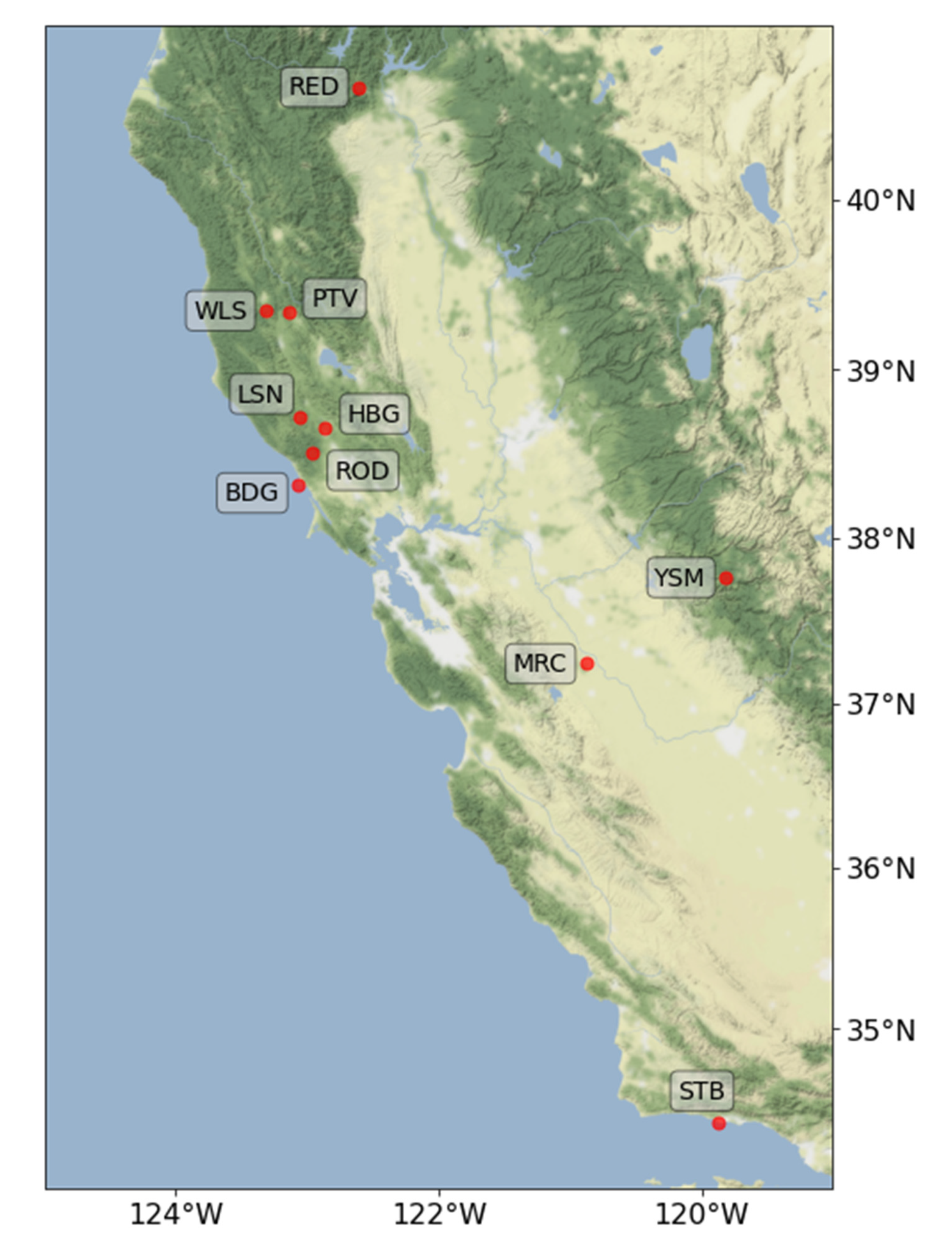
The empirical model we build is based on data from 10 land stations, located primarily in northern California. We draw from two soil networks to maximize coverage in the region: the NOAA Hydrometeorological Testbed (HMT), where five stations are used from the Russian River Valley, and the United States Climate Reference Network (CRN) as provided by the National Soil Moisture Network, which yields five additional stations (see Figure 1 for the locations of each station and Table 1 for their names and aliases). We also include an observing station in Santa Barbara even though it does not fall in the typically defined region of “northern” California as a means to increase data availability. We will see later that this is also a strategic choice for increasing predictability in the model. Both networks have undergone rigorous levels of quality control [16,36,37], and though they use different instruments, their behavior is found to be consistent enough to warrant their combination here.
To maintain consistency between networks, all soil observations were taken at a depth of 10 cm for the period 23 May 2012 to 31 December 2017. Hourly data from the HMT network were averaged to the daily scale so as to match the temporal resolution of the CRN data. The average annual cycles in soil moisture and temperature were then calculated for each of the 10 stations independently and removed linearly from the relevant time series to isolate soil anomalies, which better capture the moisture/temperature variations than the full field itself.
Though our primary interest is in the predictability of soil moisture, soil temperature is used in addition to describe the field evolution. That is, the model we build here is based on a combination of both metrics rather than on soil moisture alone to lend additional predictive capacity. However, since these two characteristics vary with different magnitudes, we make use of their z-scores for the remainder of this analysis to allow similar contributions from each to the empirical model.
Combining soil temperature and moisture in one form or another is not a unique feature of this study; soil temperature has in fact often been used as a means of deriving soil moisture. The novelty here is that we use the moisture to remove redundant information in soil temperature, which is found to improve the predictability of the moisture field itself. A linear regression is thus carried out to isolate only the temperature residual, removing the portion of the field that is already explained by soil moisture. Thus, greater weight is given to the independent information that is found in soil temperature rather than double-counting the variability common to both soil properties. The matrix of daily, anomalous, soil temperature residuals is then combined with soil moisture to build a linear inverse model as described below.
The period of 23 May 2012–31 December 2017 was long enough to allow data denial experiments for some exploration of prediction skill. However, the entire period was employed for diagnosing skillful ICs and for hindcast experiments to measure potential predictability.
2.2. Linear Inverse Modeling: Background
We outline here the key steps used in creating the soil model, but refer the reader to previous studies for a more detailed description of LIM and the theory behind it (e.g., [8,17,20,21], and to Appendix A for more information on the application of it here. To apply LIM, we assume that the system is linear with the relevant dynamics separated on the basis of time scales; one dynamic component—the predictable part—must occur on timescales slow enough relative the rest of the field, which varies on timescales fast enough that it can be described as unresolved stochasticity. This allows the system to be reasonably well approximated by a stochastic differential equation of the form:
where i is the time series of soil temperature or moisture at each station i, and Lij is the linear operator describing the predictability of conditions at station i stemming from knowledge of conditions at stations j. The matrix S contains the coefficients for the vector of white noise forcing, , with the individual components of white noise subscripted α. The second term on the right-hand side of Equation (1) is described in terms of the noise covariance matrix, Q:
For simplicity, we assume in the following that Q is independent of , though this may not be the case everywhere. After all, there is evidence that soil moisture may affect phenomena such as precipitation [38], which are assumed to be included in the stochastic forcing. In any case, the procedure we outline here results from deriving the best linear predictions of in the mean squared sense [18].
Given these assumptions, the matrices L and Q describe the dynamics of the system and its evolution. Their values can be determined by starting with the appropriate Fokker-Plank Equation (FPE) associated with Equation (1):
where describes the conditional probability of finding a value at a certain time, (t), given the initial condition (0). This is also called the forecast probability. When the temporal derivative on the left-hand side of Equation (3) is set to zero, the resulting stationary FPE is satisfied by the stationary probability . Taking the moments of these FPEs allows estimation of the lagged covariance matrix given lag and the contemporaneous covariance matrix , which can be combined to form the Green function as follows:
This matrix is called the Green function because for systems governed by Equation (1) it is equivalent to exp(L) and, when operated on an initial condition (0), provides the vector () at which the forecast probability is maximized. That is, given Equation (1) with constant L and Q, is Gaussian centered on , making the most likely forecast at lead time given initial condition . For long lead times, the forecast probability converges to the centered stationary probability .
Details of how the eigenstructure of can be used to estimate matrices L and Q are given in Appendix A. These matrices are important in diagnosing the dynamical system generating the measured field , and we shall consider them in detail for the system analyzed here in Section 3.4. For now, we turn our attention to the use of LIM for forecasting.
2.3. Linear Inverse Modeling: Forecasts
For many measured quantities, the estimate of the stationary probability distribution given by the histogram of measurements is in fact not Gaussian. We shall see that this is true for soil moisture in which case the forecast probabilities are not Gaussian, either. Nevertheless, it can be shown that the best linear forecast of in the mean square sense [18] is in fact still given by , with estimated as in Equation (4).
However, using Equation (4) to estimate the Green function at every lead time for which a forecast is desired is neither more nor less than forecasting by multiple linear regression. We require more than such forecasts; we require an estimation of how good the approximation in Equation (1) is to the true dynamics of the system and a prioi estimates of the expected forecast error. Appendix A provides a method for estimating Green functions at other leads estimated from the original matrix . If Equation (1) is valid, then is theoretically independent of (the tau test: [8,17]; Appendix A). In practice, issues such as undersampling, Nyquist problems that arise when is roughly half the period of an oscillation internal to the system [39], and omission of relevant variables can all cause failure of the tau test, even when Equation (1) is valid. Nevertheless, the better the tau test is passed (with “better” being defined by the user), the better Equation (1) is as an approximation to the real system.
In this study, we shall apply the tau test and also estimate the expected forecast error by considering the theoretically expected mean-square forecast error using Green functions :
In Equation (5), angle brackets indicate an average over ICs or verifications Note that if is strongly dependent on , then so is , indicating that the tau test fails. In the remainder of Section 2, we shall assume that the tau test is passed and drop the argument from our notation of the estimated Green function, henceforth denoted as .
2.4. Linear Inverse Modeling: Forecasts of Opportunity
Clearly, not all forecasts have equal skill. We note from the last section that in this particular model, the only entity varying from forecast to forecast is the initial condition. Thus, since knowing when soils are likely to be anomalously wet or dry could be linked to increased predictability for floods or droughts, we would like to identify a class of ICs for which forecasts may be expected in advance to be unusually skillful. To look for these “forecasts of opportunity”, we first ask a different question: what initial condition leads to the forecast at lead with the largest amplitude? This initial condition, or “optimal structure” (defined below), has been explored by many authors [8,40,41,42,43,44] as a mechanism for growth, called “optimal growth,” in geophysical systems. A brief description of optimal growth is provided here while a more detailed discussion is provided in Appendix B.
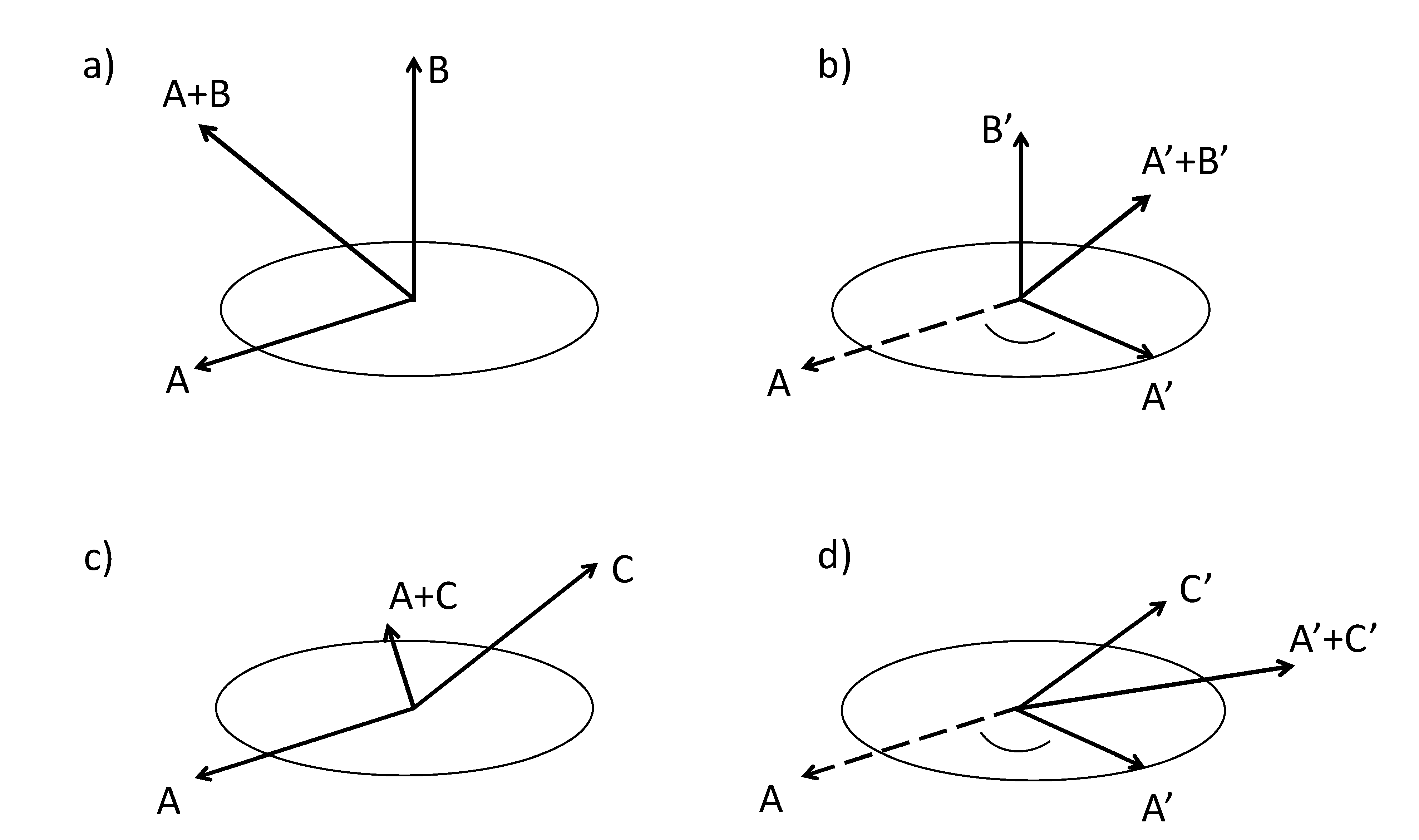
Optimal growth occurs when the eigenvectors of a linear system (i.e., their modes) are not orthogonal. The modes of L in Equation (1) all correspond to eigenvalues with negative real parts. Without forcing, then, the time series coefficients of these modes decay exponentially. However, because the imaginary parts of the eigenvalues are generally nonzero, and modes themselves are not orthogonal, the amplitude of the system as a whole can temporarily grow even without forcing. To illustrate, consider a system with three modes corresponding to a purely decaying eigenvalue and to a complex conjugate pair, as illustrated in Figure 2. The complex conjugate pair of modes is basically the same physical mode, but requires two degrees of freedom to describe it. In Figure 2a, the vector A represents the length of the complex mode and vector B represents the purely decaying mode, orthogonal to A. After some time, A has rotated and decayed to A’, and B has decayed to B’ (Figure 2b). The vector sum A’ + B’ now has a smaller magnitude than the initial condition A + B. Now consider Figure 2c, showing the same complex mode A, but another purely decaying mode C, which is the same length as B but is not orthogonal to A. After some time, C has decayed to C’ having the same length and decay time as B’, and A has decayed to A’ as before (Figure 2d). However, the magnitude of A’ + C’ is now larger than that of the initial condition A + C. Of course, without forcing, the modes will continue to decay and so this growth is only temporary.
In our model, the only forcing is stochastic. Thus, any predictable growth in the system is of this non-normal type. The optimal structure is then the initial condition consisting of the optimal combination of modes leading to the maximum amount of growth. As discussed in Appendix B, the optimal structure 1 for a forecast at lead is the leading eigenvector of , and the variance of the forecast field is amplified over the variance of by a factor given by the corresponding eigenvalue . Typically, a graph of vs. has a maximum at lead time peak; this curve is thus called the Maximum Amplification Curve.
Having estimated an optimal structure, which we normalize to unity, it is possible to generate a histogram of projections of the observed field onto the structure of . In previous studies involving LIM forecasts (e.g., [9,10,11] it has been shown that forecasts based on ICs with strong positive or negative projections onto 1 are also the most skillful. Recalling that each vector in the timeseries is a candidate initial condition, we shall show that ICs in the upper tercile of the histogram of |(t)| are indeed more skillful than other forecasts; forecasts based on this class of ICs are therefore called “forecasts of opportunity in the field norm,” consistent with previous work cited here.
In this study, we are less interested in forecasts of the combined soil temperature and soil moisture field than in forecasts of the soil moisture by itself. We do, however, wish to take advantage of whatever additional predictability soil temperature can give forecasts of moisture. It is possible to find an optimal structure which maximizes the growth of moisture alone, regardless of how soil temperature evolves, by employing a “moisture norm” N that excludes forecasts of temperature from estimation of the optimal structure. That is, we use a procedure identical to that discussed above with the modification that the optimal structure in the moisture norm is the leading eigenvector M of , corresponding to leading eigenvalue . As with the field norm, forecasts of opportunity in the moisture norm are based on ICs with relatively strong values of |(t)|.
3. Results
3.1. Test of the Linearity Assumption and Field-Wide Anomaly Amplification
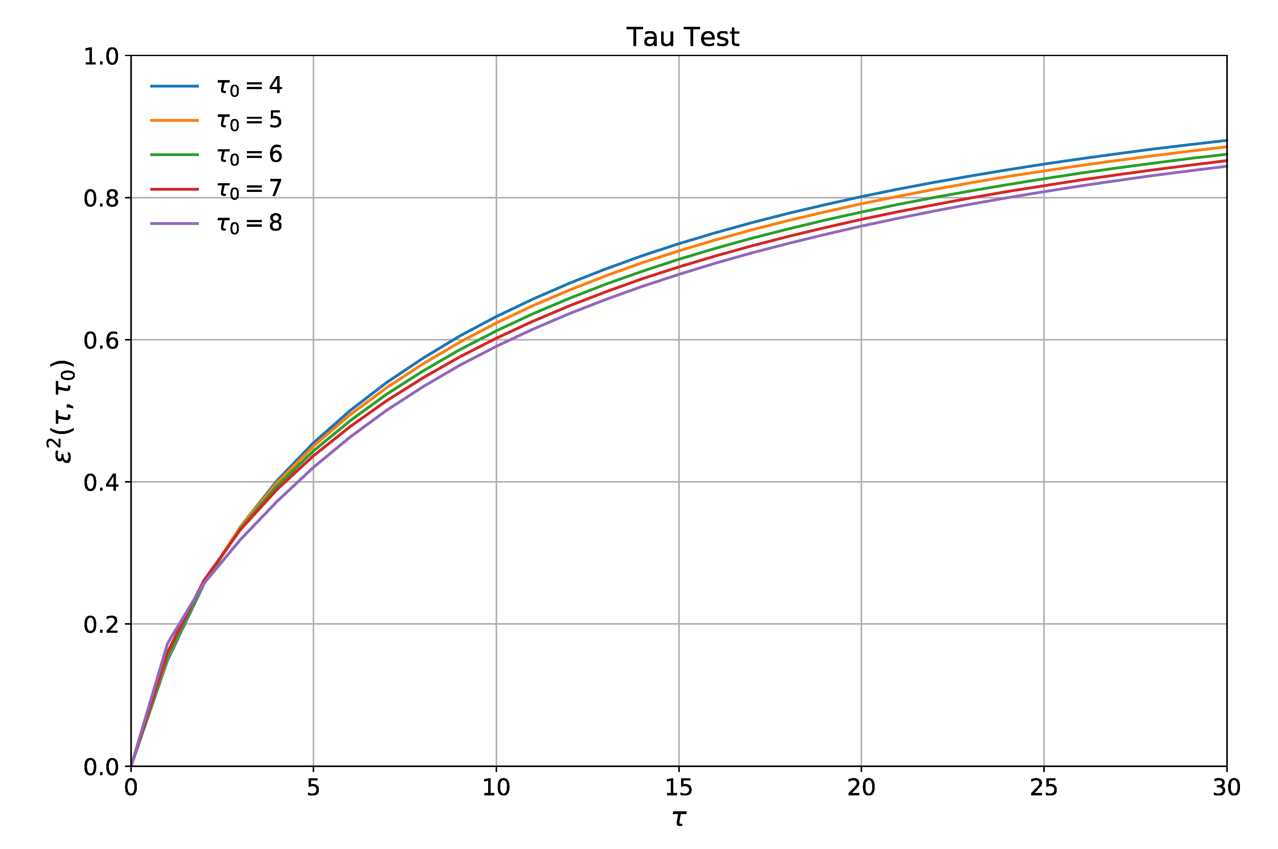
Before assessing the model in detail and its performance relative to observations, we first confirm the validity of applying LIM to the selected set of soil data by employing a tau test as described above (Figure 3; see Section 2.3). We have estimated for lags between four and eight days, and estimated the LIM forecast error as in Equation (5) out to a lead of 30 days (with day zero having zero error). Although there is a small amount of separation between each of the five values as grows, the expected errors remain similar enough that we consider the system to be roughly linear, or at least linearized on these timescales. The choice of a linear model to describe the combined fields of soil temperature and moisture is thus a reasonable one. In order to avoid sensitivities that arise as we approach a Nyquist mode at eight days (see [39]), we will use a value of seven days for moving forward.
Interacting oscillatory modes that can lead to temporary growth in the system (as illustrated in Figure 2) are the eigenvectors of . Characteristics of these modes are given in Table 2. We note that these eigenvectors represent the predictable component of field evolution, as they are identical to those of L. Each mode in this system is noticeably damped; that is, the decay time of the oscillation is much less than its period. This suggests that if each mode acted in isolation from the others and decayed individually, the system as a whole would decay as well. However, their non-normal interactions allow for the field to grow instead.
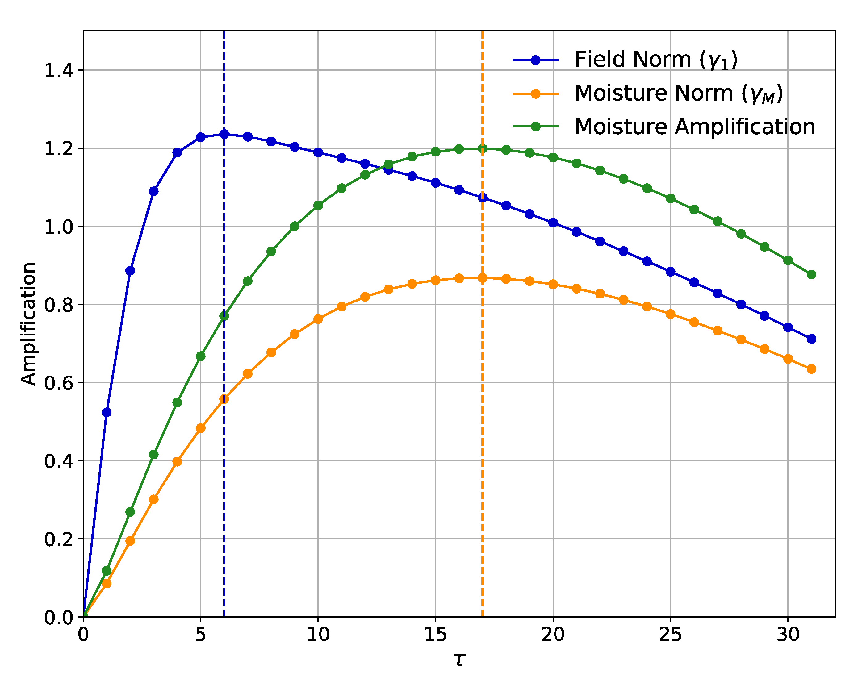
The next step is then to determine the lead time at which the maximum amount of growth in the field occurs, denoted here as , by constructing curves of vs. (the Maximum Amplification Curve) and vs. (Figure 4). We present this curve for both the field and moisture norm, but note that the field norm shows amplification of the full field (soil temperature and moisture) over the initial condition while the moisture norm shows only the variance of the soil moisture prediction compared with the variance of the entire initial condition, including temperature (see Appendix B for details on each norm). Additionally, shown in Figure 4 is the actual amplification of the soil moisture field by itself, i.e., the variance of the soil moisture prediction compared with the variance of soil moisture contribution to the optimal initial structure. Using the moisture norm thus extends predictability of maximum growth from = 6 days to = 17 days. This suggests that given an ideal set of ICs (the “optimal structure”), growth of soil moisture could peak near a two-week lead time. The next question then is what does that set of ICs look like that leads to this level of growth, and does it actually occur in the dataset?
3.2. Optimal Structure and Multi-Week Forecasts of Soil Conditions
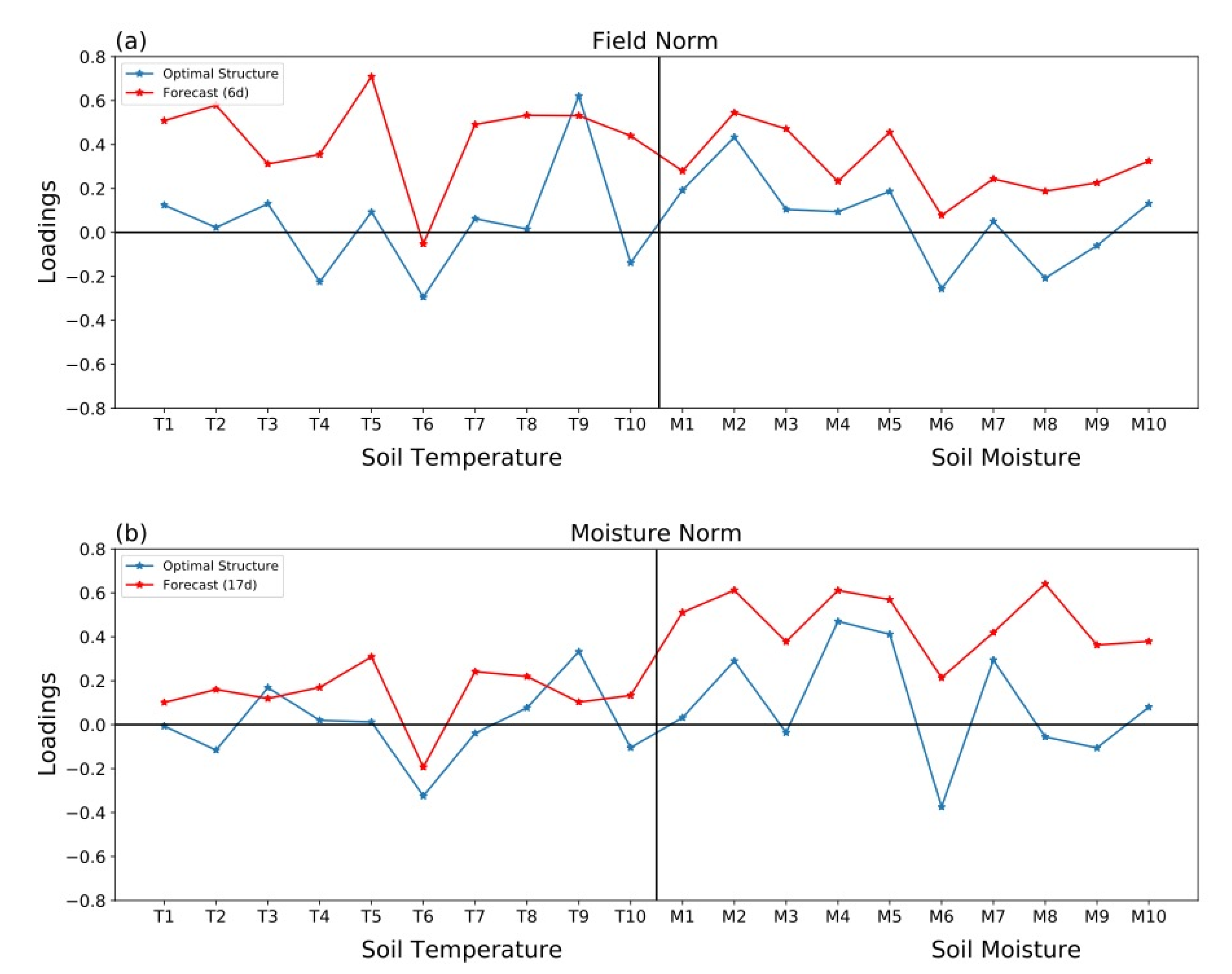
The optimal structure describes the set of ICs that lead to the maximum amount of growth in the field (Figure 5, blue line); when it is operated on by , the forecast soil conditions after days can also be estimated (Figure 5, red line; see Section 2.4 and Appendix B for details). Optimal structures and their evolution after days are presented in Figure 5 for both the field norm (top) and moisture norm (bottom). When interpreting these plots of optimal structures and their evolved structures after days, the sign of the soil anomaly is dependent on the sign of the loading (the station’s contribution to or ), while the absolute value of the loading indicates the magnitude of that anomaly. From this, it becomes clear that not all stations contribute equally to the optimal set of ICs. That is, some stations have larger loadings than others. For example, T9 (STB) stands out in the soil temperature portion of the model as contributing strongly to the optimal structure regardless of whether the field or moisture norm is applied.
A strong contribution to the optimal structure from a certain station does not guarantee that a large amount of actual growth will occur there (the magnitude of which is determined by the distance between the red and blue lines in Figure 5). Let us return for example to T9′s (STB’s) role in soil temperature evolution. Unlike T9, T5 (WLS) is not an important contributor to the optimal set of ICs that prime the field for growth, yet it is the station that experiences the largest change in soil temperature under the field norm. In the moisture norm, T9 (STB) temperature anomalies are actually forecast to decrease after 17 days. Similarly for soil moisture, M4 (ROD) and M5 (WLS) play a strong role in terms of the optimal structure but it is M8 (RED) showing the largest increase after days. We will return to an assessment of station-dependent contributions to the field evolution in Section 3.4, but first we focus on the soil moisture forecasts themselves. We can see in Figure 5 that the forecasts at each site likely vary in magnitude, but this tells us nothing of the forecast skill.
3.3. Forecasts of Opportunity
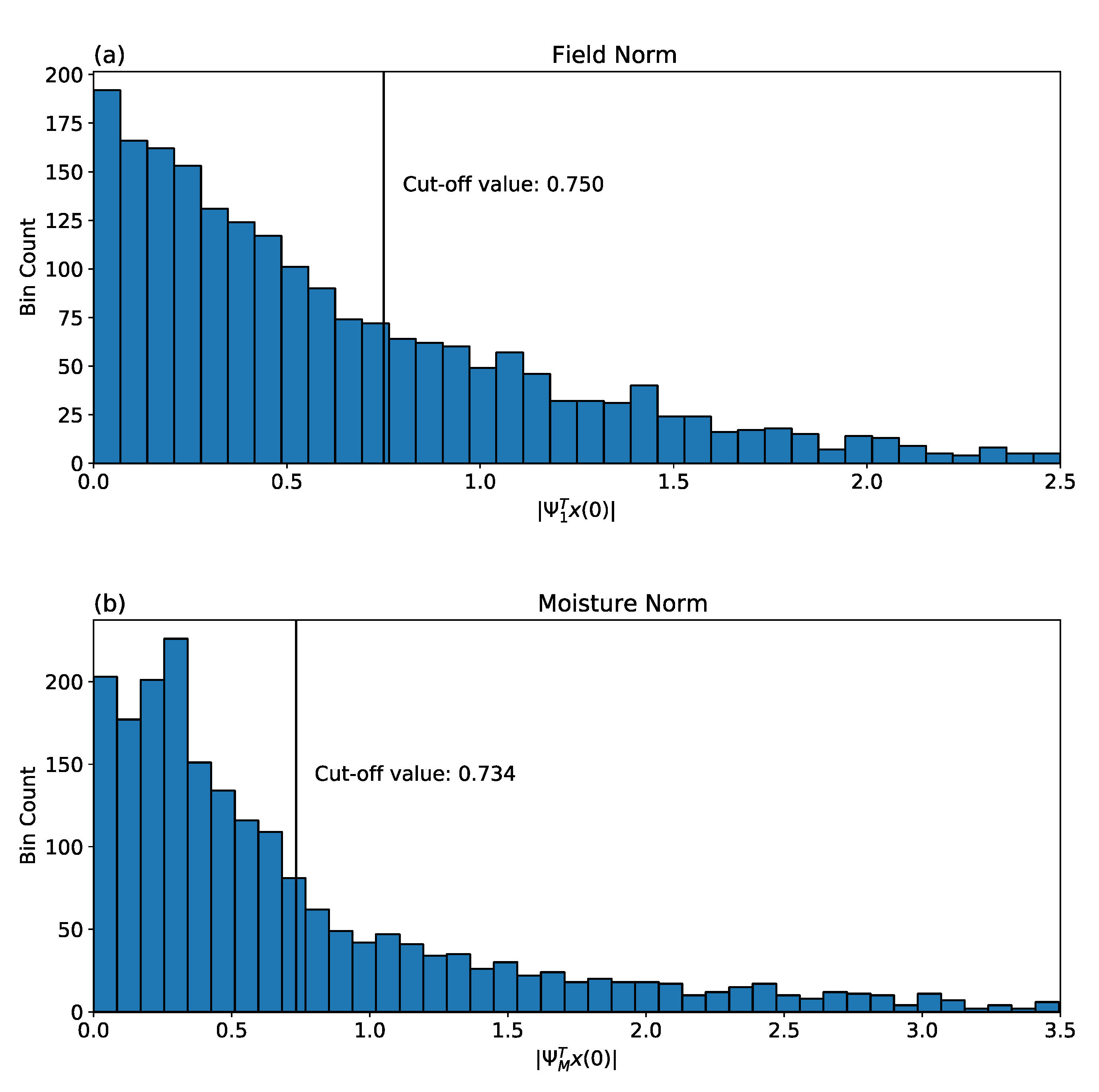
As discussed in Section 2.4, for a forecast to be truly useful it must have some estimate of the confidence associated with it prior to its verification against reality. The LIM approach used here enables just that, as the expected forecast errors are produced a priori as in Equation (5). However, there is another critical benefit of this method—it allows for the identification of forecasts of opportunity based on how strongly the ICs on any given day agree with the optimal structure. We define a value for the projection of (or , depending on which norm is selected) onto the observations (i.e., candidate ICs) above which we expect particularly skillful forecasts. In this case, we define that cutoff as the top tercile of the magnitude of that projection for the field and moisture norms separately (Figure 6). Though the chosen threshold is somewhat arbitrary, we show in Figure 7 that it increases skill as expected.
We assess how well the forecasts of soil moisture, whether conditioned on this upper tercile of ICs or covering the entire record, perform relative to verifications. As explained above, we first look at hindcasts of dependent data and interpret the results as an indication of potential skill. Below, we present data denial experiments to estimate independent skill. Even in hindcast experiments, though, we can compare the potential skill in the LIM-generated forecasts relative to that of an AR1 process whose prediction is based solely on the preceding value of the field at a particular location as some level of performance benchmark.
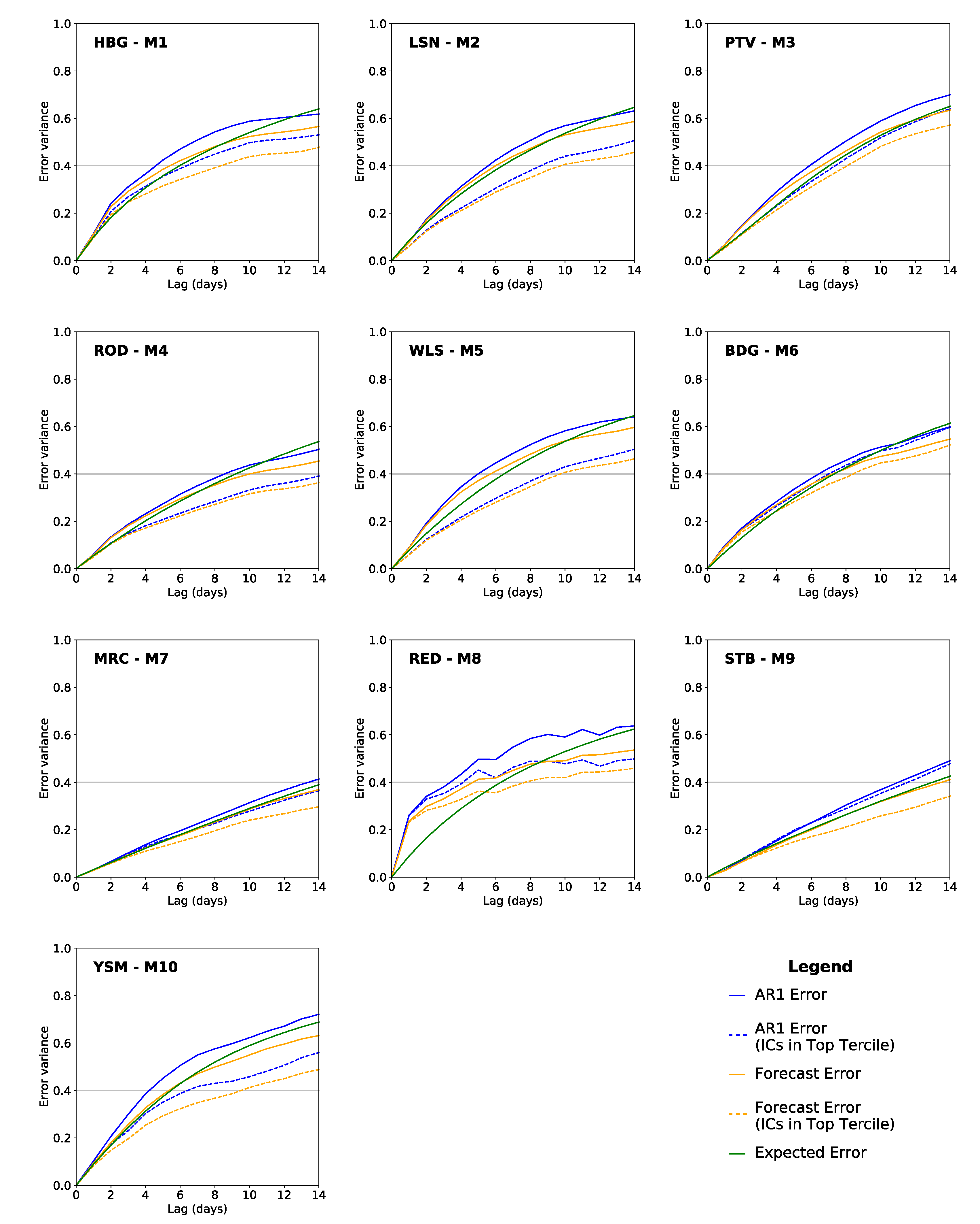
The mean square error (MSE) of these soil moisture hindcasts, normalized to the variance of verifications, as well as the a priori expected error estimates from LIM, are shown in Figure 7 for the moisture norm out to a 2-week lead time. We consider skill to be maintained in the hindcast if the normalized error variance remains below 0.4. This is again a somewhat subjective choice, but is rooted in practical forecasting (not discussed in detail here).
For all 10 stations, the error associated with the soil moisture hindcast in LIM is consistently lower than that associated with an AR1 process from days 2–3 onwards (orange vs. blue lines in Figure 7). In other words, the predictions of soil moisture that are generated in this new empirical model out-perform persistence-style forecasts on time scales of a few days to a few weeks, depending on location.
That performance can increase further by considering forecasts of opportunity (solid vs. dashed lines in Figure 7). With this definition, skill in the hindcasts is maintained for as long as 20 days at MRC, 17 days at STB, and 16 days at ROD (not shown). At minimum, skill is maintained across all stations for 8 days when conditioned on this upper tercile of ICs. Note also that a priori estimates of skill (green lines) provide useful indications of actual skill; i.e., the green line typically agrees with the solid orange line across all stations.
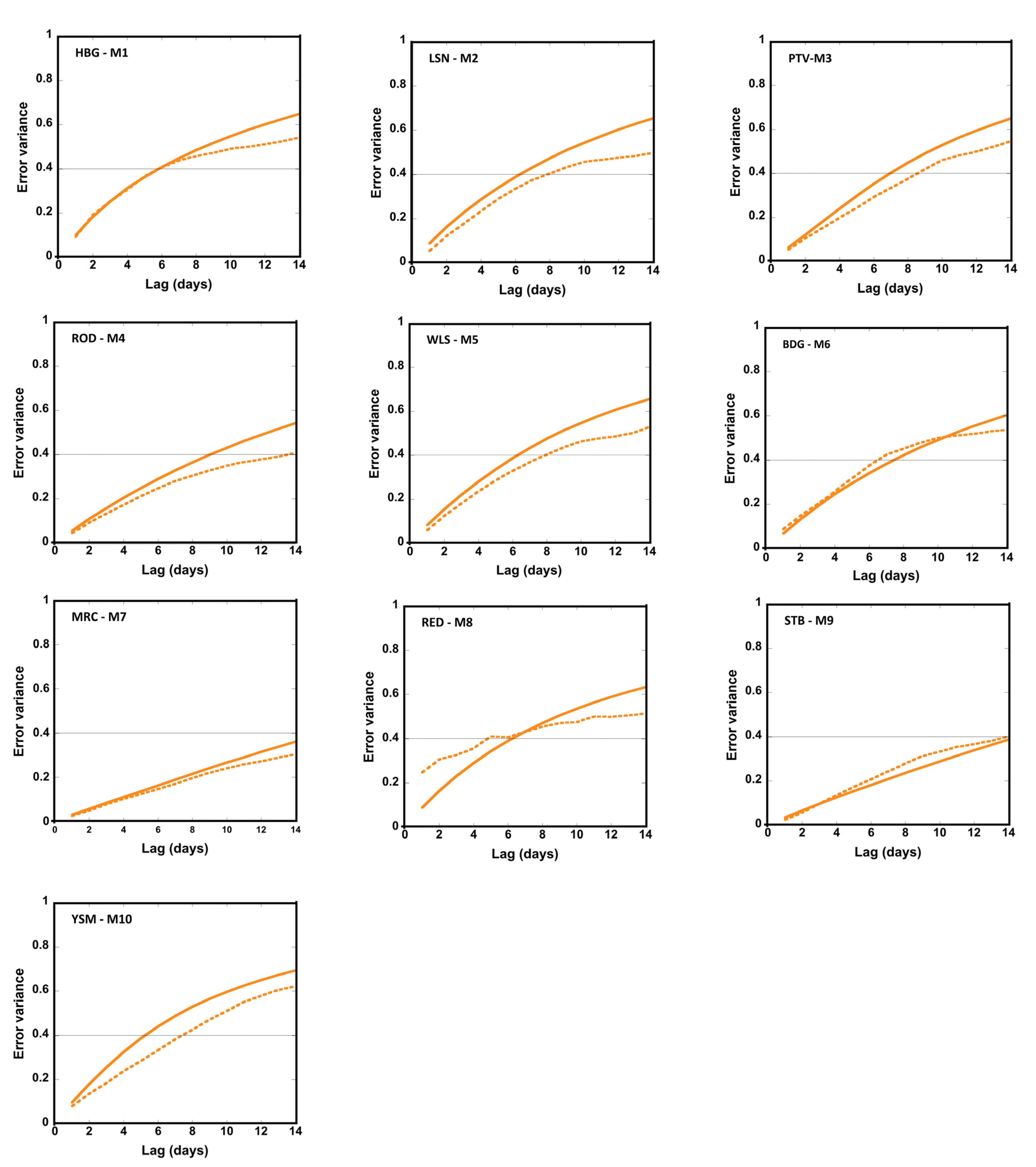
Although the data set is so short that withholding a year of it greatly increases the noise in the results, we require knowing whether independent forecasts are similar to those we have presented thus far for diagnostic purposes. For this reason, we did withhold one year of data at a time, for five years, estimate the Green functions from the retained values for each of the five years, and average the moisture forecast errors estimated from the five verification periods. Recall that the calendar year in California bisects the rainy period, and so our withheld years began on 23rd May and ended on 22nd May. Using the moisture norm, the optimal structures from these analyses (not shown), being highly derived quantities, are extremely noisy. All of them, however, agree in having their largest loadings (absolute value > 0.2) as shown for the entire data set in Figure 5b at T6, T9, M2, M4 and M5. Most of them also have large loadings at M6 and M7. For a field of 20 predictors, randomly distributed loadings of 0.05 to 0.1 would be expected. Given this level of consistency with the optimal structure shown in Figure 5b, we decided to use the same ICs as forecasts of opportunity for moisture as used in Figure 7. We emphasize that although the selection of ICs was based on the entire data set, the forecasts were verified on values independent of data used to estimate the predictor Green functions.
The independent error variance of moisture forecasts, normalized to the variance of the verification field, is shown in Figure 8. With some differences, Figure 8 tells the same basic story as Figure 7; ICs in the upper tercile of the projections onto the optimal structure are consistently more skillful than the others. It is also gratifying to note that the moisture forecast errors in Figure 8 are similar to the hindcast errors verified on dependent data in regard to their temporal evolution.
We have thus far suggested an optimal structure that has the potential to lead to substantial amounts of soil moisture growth on the order of two weeks with hindcasts that maintain skill on similar timescales, but it is also important to determine how often these conditions actually appear in nature. We thus seek to understand how much variance in the field is captured by the optimal structure in Figure 5. We apply a Euclidean norm to the forecast structures based on and individually, and assess the ratio of ) to to isolate the portion of inter-station variance captured by LIM either across the whole field, or modified to consider only soil moisture. When using the field norm, about 27.4% of the variance in soil temperature and moisture can be explained. However, the moisture norm can explain as much as 50.8% of the variance in soil moisture alone. This structure thus captures a non-negligible portion of the variance that has been observed to occur in nature. Given this and the above evidence on the model’s skillful hindcasts of soil moisture, we argue that LIM is a valuable tool for advancing the state of multi-week forecasts of soil conditions.
3.4. Assessing the Predictable and Stochastic Portions of Field Evolution
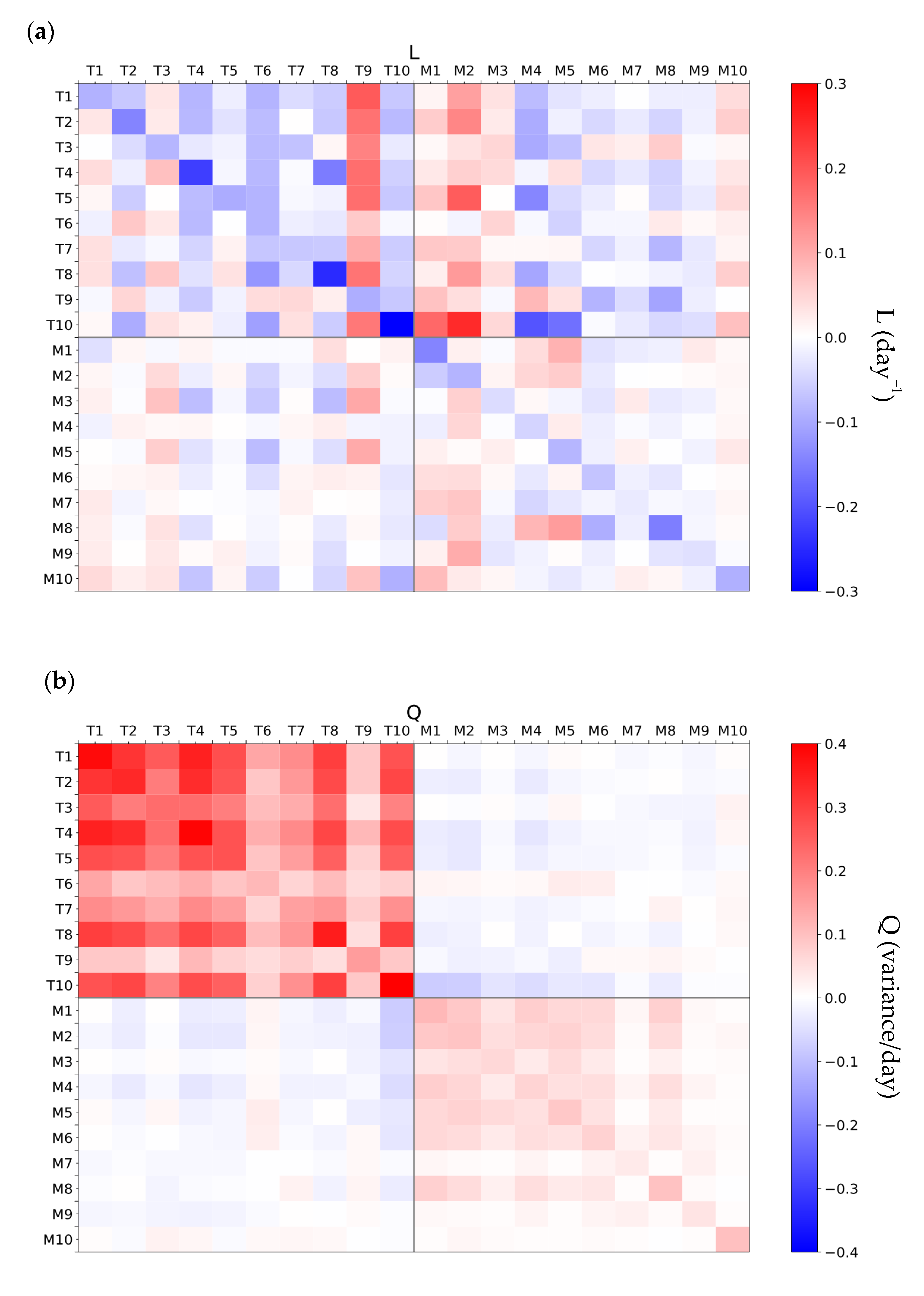
At present, it remains unclear why certain stations play a more dominant role in the optimal structure or respond more strongly in the forecast, though it could be due to a number of factors—distance from the coast and thus exposure to incoming storms, latitude, elevation, soil type, vegetation cover, etc. However, additional information about the system may be gleaned by investigating the model’s L and Q matrices in Equations (1) and (2), corresponding to the predictable component of evolution and the unresolved stochastic portions of the field, respectively. Heatmaps of both are presented in Figure 9. For easing interpretation of these plots: the top left quadrant shows the contribution of temperature at each station to another station’s temperature trends; the top right quadrant shows the contribution of station moisture to station temperature trends; the bottom left shows the contribution of station temperature to the soil moisture trend; and the bottom right shows the contribution of moisture to other stations’ moisture trends.
Let us first consider the slower evolving dynamics of the system characterized by L (Figure 9a). One feature that stands out immediately is the strong negative diagonal component, which is to be expected—each station is most strongly reactive to local influences, and the anomalies at each station tend to decay back to some equilibrium when considered individually. However, less obvious properties emerge as well. T9 (STB) for example, again stands out for the ability of its soil temperature to predict temperature trends at other stations as well, indicated by the vertical column of positive values for T9 in the top left quadrant. For the case of residual soil temperatures then, northern station predictability may stem in large part from considering the conditions to their south. Soil moisture at M2 (LSN) also appears to indicate increasing anomalies in soil temperature trends at a number of stations (mostly positive values for this column in the top right quadrant), though these patterns are somewhat less consistent in magnitude across each station relative to the those of T9. However, strong negative values are important to consider as well. Soil moisture at T6 (WLS), for instance, implies damping of both temperature and moisture anomalies at a number of other stations.
Turning now to the more rapidly evolving dynamics of the system, station dominance in L again does not correspond to similar dominance in Q (Figure 9b). On the contrary, the soil temperature forcing of STB actually stands out for its lack of correlation with stochastic forcing of temperature at other stations (light red column under T9 in the top left quadrant). However, the most apparent facet of Q is that the unresolved stochasticity is generated primarily by the soil temperature portion of the field (largest values in the top left quadrant). Soil moisture contributes more weakly than temperature to the rapidly varying forcing (smaller values in the bottom right quadrant). The off-diagonal quadrants in the upper left and bottom right of Figure 8 are generally weaker as well, and primarily negative. This suggests that the moisture and temperature forcings are anti-correlated so that a higher temperature forcing implies soil moisture forcing in the opposite direction, consistent with our physical understanding of soil evolution.
The contribution of the stochastic forcing to the optimal structure was also examined, and found to be small regardless of whether the field or moisture norm is used (not shown). This leads us to hope that the optimal structure itself may then be predictable to some extent, using a method yet to be developed. If those conditions can be predicted well enough in advance, this could increase the lead time of skillful soil moisture forecasts further.
4. Conclusions and Discussion
Accurate forecasts of soil moisture have the potential to advance the forecasting of floods and flash droughts, and could offer tangible benefits for reservoir and agricultural operations. However, prior attempts to craft these predictions have been hampered by a reliance on imprecise model data, unsatisfying parameterizations of soil and vegetation properties, and/or the necessity of careful site-specific model calibration. Here, we test the predictability of soil moisture using an approach new to the field of terrestrial hydrologic forecasting, linear inverse modeling, which has been used for a number of years in oceanic and atmospheric topics [8,20,21,22,23].
The application of LIM in this context is shown to maintain skill in soil moisture hindcasts for lead times of 1–2 weeks when built on observations of soil temperature and moisture across a network of 10 stations in California. That skill can be extended by utilizing a critical piece of information produced by the model: the optimal structure. This is the set of ICs at each station that would lead to the maximum amount of growth in soil anomalies, and when projected onto the observed ICs can give an estimate of how good the forecast will be at the time of its creation. We thus follow in the footsteps of previous studies [9,10,11] to identify forecasts of opportunity; if the magnitude of that projection is in the upper tercile of all those observed, the forecast is expected to have higher than average skill. Indeed, this approach extends the length of time for which forecast skill can be maintained in an MSE sense, ranging from 8–20 days between stations. Those ICs that fall into this upper tercile offer additional avenues for further exploration to better understand which synoptic conditions tend to create these opportunities and their potential for acting as early warnings of highly anomalous soil moisture conditions.
The timescale of predictability found here when using only direct, in-ground measurements of soil temperature and moisture align well with previous predictability studies. [13], using a soil water balance model and observed forcings (i.e., precipitation, evapotranspiration, etc.), found that soil moisture could be skillfully forecast to a one-week lead time in Switzerland. They also note that incorporating additional information, such as snow melt or seasonal forecasts of relevant moisture forcing, could double that predictability time scale. Incorporating additional environmental variables in this manner may thus improve the predictability estimated by LIM, but we have chosen to focus here on establishing a baseline for the internal predictability of the system without including atmospheric forcing as a predictor.
There are additional opportunities to refine and improve the model introduced here, as well. In the course of assessing the underlying soil temperature and moisture data used to build this LIM, it was found that while soil temperature residuals are roughly Gaussian, soil moisture as a whole is in fact strongly non-Gaussian (not shown). The model created here may thus benefit from accounting for the non-Gaussian nature of moisture itself, potentially through considering combinations of additive and multiplicative noise. This does, however, complicate the model and its implementation and is thus reserved for future analysis.
The results presented above thus represent only the first step in improving our predictions of soil moisture evolution in California. There are a number of features in this model that deserve to be explored more fully. Why do certain stations play a larger role than others in determining the growth of the field? Why do some grow more strongly than others after days? Which environmental factors are the driving forces behind the slow and fast growth components of the model? Additional considerations expand beyond just this region and model—does this type of analysis perform similarly well in other California regions, such as the Sierra Nevada range? Can we expand to different states, and what are the scale limitations on data inclusion in a single application of LIM? Additionally, perhaps most importantly, how can these forecasts be most usefully employed to benefit stakeholders in the region?
As in any modeling study, the above results are limited by a number of factors. The length of each station’s soil record has regrettably hampered some of our efforts to understand soil moisture in the region, and in particular limits model validation efforts. Quality can also be an issue. For this reason, we have been selective (at least to the extent possible in the face of limited data) in which observations are used and rely only on well quality-controlled data. Future studies may benefit by assessing the sensitivity of results when incorporating remotely sensed or modeled data.
By construction, LIM also simplifies the driving forces behind soil moisture growth and decay into two single matrices, L and Q; there is not a quick and easy way to determine when rainfall, soil properties, or plant function are the primary culprit for altering soil conditions. That said, there does exist the potential to diagnose the stochastic forcing, Q, through temporally higher resolution observations and/or model output [45]. Though these are all critical things to consider and a number of tasks remain to be accomplished, we reserve such for future work in the interest of first introducing an innovative method for producing realistic estimates of soil conditions on multi-week timescales.
We suggest that the performance of LIM shown here is a strong argument for further exploring its use in the context of soil moisture predictability. One particularly interesting avenue for future exploration pertains to the ability of numerical models to capture similar features of predictability as those shown here. We hope these initial observational results will inspire researchers to assess soil moisture evolution in numerical models, including NOAA’s National Water Model [46]. By applying the same LIM approach to model output as we did to observations, one has the opportunity to investigate how well the model captures realistic soil moisture growth, at least at a series of point-based measurements. Because of the increased spatial coverage and length of model-derived data, one can also investigate the effects of increasing spatiotemporal resolution on soil moisture predictability in this manner.
Soil moisture forecasting, particularly in the western United States, is a topic likely to continue growing in importance as climate variability increases and the threat of more frequent/intense hydrometeorological extremes looms larger in the coming decades [47,48]. In the face of these changes, LIM is uniquely situated to aid the development of simple and adaptable approaches to understanding soil moisture anomaly growth using observations and/or model output in these critical regions.
Author Contributions
Conceptualization: C.P. and R.C. Methodology: C.P. Software: M.D.F. and C.P. Formal analysis: C.P. and M.D.F. Resources: D.L.J. and R.C. Data curation: D.L.J. and M.D.F. Writing—original draft preparation: M.D.F. and C.P. Writing—review and editing: C.P., M.D.F., D.L.J. and R.C. Visualization: M.D.F. and D.L.J. All authors have read and agreed to the published version of the manuscript.
Funding
This work is supported by the National Oceanic and Atmospheric Administration’s (NOAA) Office of Water and Air Quality (OWAQ) program, forecasting a Continuum of Environmental Threats (FACETs).
Institutional Review Board Statement
Not applicable.
Informed Consent Statement
Not applicable.
Acknowledgments
The authors thank Bob Zamora and Daniel Gottas for their assistance in accessing and processing the soil data used here. We also thank Roger Pulwarty for valuable discussions, for introducing us to the FACETs program, and for assisting with the grant writing. This work is supported by the National Oceanic and Atmospheric Administration’s (NOAA) Office of Water and Air Quality FACETs program.
Conflicts of Interest
The authors declare no conflict of interest in this work.
Appendix A
Review of Linear Inverse Modeling
When applying Linear Inverse Modeling (LIM), we first assume that the dynamics of a zero-mean state vector x(t) is governed by a linear Markov process:
where L is the linear operator that describes the slow evolution of the field (the “predictable” part), and S is the matrix of coefficients for the vector of Gaussian white noise forcing, . Here, both L and S are constant matrices. The second term on the right-hand side of Equation (A1) is described in terms of the noise covariance matrix, Q:
Using the Fokker-Planck equation (Equation (3) in the text), we find that for some time interval
with Equation (A3) equivalent to Equation (4) in the text. Since the solution to Equation (3) for any lead
is Gaussian centered on exp(L), the mean of this forecast probability is also the most likely forecast given initial condition . We therefore identify exp(L) with the Green function, labeling it .
We estimate the Green function at any lead by choosing a particular and estimating from Equation (A3). The set of eigenvectors, or modes, {uα} of correspond to eigenvalues {gα}. The exponential relationship between and L requires that and L have the same set of modes. and LT also have the same set of eigenvectors, called adjoints, {vα}. If a mode uα corresponds to eigenvalue gα, then adjoint vα corresponds to that same eigenvalue. With proper normalization, the modes and adjoints form a biorthogonal set:
Equations (4) and (5) allow us to write and L in terms of their modal decomposition:
Since gα( is a scalar, we may use Equations (A5) and (A6a) to estimate the Green function at any lag from as
Because and L are real, the modes {uα} along with their corresponding adjoints and eigenvalues are either real or occur in complex conjugate pairs. The implications of this are discussed in the text and in Appendix B.
If Equation (A1) is valid, then should be independent of . In practical applications, this “tau test” is sometimes failed even when Equation (A1) is valid. Spurious failure may be due to insufficient data, Nyquist issues (not discussed here; see [39]), or observation errors.
We note that LIM can be partially extended to account for systems like Equation (A1), but where S is a linear function of rather than a constant matrix. That is,
where ηα and are independent Gaussian white noises. Without going into details (but see [49,50]), the matrix L in Equation (A3) is replaced by a matrix M, where M = L + ½. If = 0, then Equation (A8) is equivalent to Equation (A1). If ≠ 0, the forecast probability is no longer Gaussian. Nevertheless, if we identify with exp(M), the best forecast in the mean square sense is still and the tau test is still passed.
It remains to use our empirical estimations to diagnose the nature of the stochastic forcing. In fact, we cannot uniquely identify S, we can only identify Q (Equation (A2)). Taking moments of the stationary FPE when S is constant yields the “fluctuation-dissipation relation”:
If S is a linear function of x as in Equation (A8), then an equation similar to Equation (A9) is obeyed, but with L replaced with M, and with Q having terms involving . In this study, since we do not have enough data to identify the additive and multiplicative noises even if were diagonal, [51], we shall use L and M interchangeably in the results section and confine our attention to the matrix Q when considering the stochastic forcing.
Appendix B
Non-Normal Growth and the Optimal Structure
As stated in the text, forecasts of opportunity are often associated with non-normal growth associated with an optimal initial condition. Identification of this “optimal structure” is made by maximizing the size of the forecast field relative to the size of the initial condition. Since the best forecast at lead using initial condition is G(τ), we maximize T relative to x(0)Tx(0) with respect to a component xm of the initial condition. Thus,
In Equation (A10) we have defined the quantity as the amplification of the squared magnitude of the forecast field over the squared magnitude of the initial condition x, dropping the arguments of x(0) and G(τ) in Equation (A10) for brevity. Evaluating Equation (A10), we find that
which is equivalent to the eigenvalue problem
where Ψ is the initial condition x(0) satisfying the Equation (A11) and γ is the corresponding amplification. The leading eigenvector Ψ1, associated with the largest eigenvalue γ1 and normalized to unity, is the optimal initial structure for growth of field variance by a factor of γ1 over a time interval τ.
G(τ)TG(τ)Ψ = Ψγ,
It is often the case that we wish to see what initial condition maximizes the growth of a subset of the entire state vector. For example, if x consists of components of both temperature and moisture, we may wish to see what combination of temperature and moisture in the initial condition maximizes the predictable growth of moisture, regardless of what happens to the temperature. In this case, we proceed as before, but this time the summation over i in Equation (A10) is performed only over those indices corresponding to moisture variables. This is equivalent to inserting a matrix norm N into Equation (A11) that projects out the forecast of the moisture variables:
G(τ)TNG(τ)ΨM = ΨMγM
We have labeled the eigenvectors and eigenvalues in Equation (A12) with the subscript M to indicated that these quantities are evaluated in the “moisture norm.” Thus, γM indicates the factor by which the moisture variables grow relative to the entire initial condition ΨM. As shown above, Ψ1 is the initial condition leading to the maximum amplification of the entire field. We thus identify the “field norm” with the case where N is equal to the identity matrix.
The leading eigenvalues obtained either with Equations (A11) or (A12) typically increase with lead time τ up to some maximum τpeak, after which they decrease again. While secondary peaks in a graph of γ1 or γM vs. τ (the Maximum Amplification Curve) are generally possible, that is not the case in our study. In the text, it is shown that the ICs projecting strongly onto optimal structures for growth over the interval τpeak are ICs leading to forecasts that are particularly skillful, called “forecasts of opportunity”.
References
- Entekhabi, D.; Rodriguez-Iturbe, I. Analytical framework for the characterization of the space-time variability of soil moisture. Adv. Water Resour. 1994, 17, 35–45. [Google Scholar] [CrossRef]
- Laio, F.; Porporato, A.; Ridolfi, L.; Rodriguez-Iturbe, I. Plants in water-controlled ecosystems: Active role in hydrologic processes and response to water stress: II. Probabilistic soil moisture dynamics. Adv. Water Resour. 2001, 24, 707–723. [Google Scholar] [CrossRef]
- Kim, S.; Jang, S.H. Analytical derivation of steady state soil water probability distribution function under rainfall forcing using cumulant expansion theory. KSCE J. Civ. Eng. 2007, 11, 227–232. [Google Scholar] [CrossRef]
- Feng, X.; Porporato, A.; Rodriguez-Iturbe, I. Stochastic soil water balance under seasonal climates. Proc. R. Soc. A: Math. Phys. Eng. Sci. 2015, 471, 20140623. [Google Scholar] [CrossRef]
- Dralle, D.N.; Thompson, S.E. A minimal probabilistic model for soil moisture in seasonally dry climates. Water Resour. Res. 2016, 52, 1507–1517. [Google Scholar] [CrossRef]
- Chen, Z.; Mohanty, B.P.; Rodriguez-Iturbe, I. Space-time modeling of soil moisture. Adv. Water Resour. 2017, 109, 343–354. [Google Scholar] [CrossRef]
- Suo, L.; Huang, M. Stochastic modelling of soil water dynamics and sustainability for three vegetation types on the Chinese Loess Plateau. Soil Res. 2019, 57, 500. [Google Scholar] [CrossRef]
- Penland, C.; Sardeshmukh, P.D. The optimal growth of tropical sea surface temperature anomalies. J. Clim. 1995, 8, 1999–2024. [Google Scholar] [CrossRef]
- Winkler, C.R.; Newman, M.; Sardeshmukh, P.D. A linear model of wintertime low-frequency variability. Part I: Formulation and forecast skill. J. Clim. 2001, 14, 4474–4494. [Google Scholar] [CrossRef]
- Albers, J.R.; Newman, M. A priori identification of skillful extratropical subseasonal forecasts. Geophys. Res. Lett. 2019, 46, 12527–12536. [Google Scholar] [CrossRef]
- Newman, M.; Sardeshmukh, P.D.; Winkler, C.R.; Whitaker, J.S. A study of subseasonal predictability. Mon. Weather Rev. 2003, 131, 1715–1732. [Google Scholar] [CrossRef]
- Jawson, S.D.; Niemann, J.D. Spatial patterns from EOF analysis of soil moisture at a large scale and their dependence on soil, land-use, and topographic properties. Adv. Water Resour. 2007, 30, 366–381. [Google Scholar] [CrossRef]
- Orth, R.; Seneviratne, S.I. Predictability of soil moisture and streamflow on subseasonal timescales: A case study. J. Geophys. Res. Atmos. 2013, 118, 10963–10979. [Google Scholar] [CrossRef]
- Dirmeyer, P.A.; Wu, J.; Norton, H.; Dorigo, W.; Quiring, S.; Ford, T.W.; Santanello, J.A.; Bosilovich, M.G.; Ek, M.B.; Koster, R.D.; et al. Confronting Weather and Climate Models with Observational Data from Soil Moisture Networks over the United States. J. Hydrometeorol. 2016, 17, 1049–1067. [Google Scholar] [CrossRef] [PubMed]
- Korres, W.; Koyama, C.N.; Fiener, P.; Schneider, K. Analysis of surface soil moisture patterns in agricultural landscapes using Empirical Orthogonal Functions. Hydrol. Earth Syst. Sci. 2010, 14, 751–764. [Google Scholar] [CrossRef] [Green Version]
- Quiring, S.M.; Ford, T.W.; Wang, J.K.; Khong, A.; Harris, E.; Lindgren, T.; Goldberg, D.W.; Li, Z. The North American Soil Moisture Database: Development and Applications. Bull. Am. Meteorol. Soc. 2016, 97, 1441–1459. [Google Scholar] [CrossRef]
- Penland, C. Random forcing and forecasting using principal oscillation pattern analysis. Mon. Weather Rev. 1989, 117, 2165–2185. [Google Scholar] [CrossRef] [Green Version]
- Hasselmann, K. PIPs and POPs-A general formalism for the reduction of dynamical systems in terms of principal Interaction Patterns and Prinicipal Oscillation Patterns. J. Geophys. Res. Space Phys. 1988, 93, 11015–11021. [Google Scholar] [CrossRef] [Green Version]
- Von Storch, H.; Bruns, T.; Fischer-Bruns, I.; Hasselmann, K. Principal oscillation pattern analysis of the 30- to 60-day oscillation in general circulation model equatorial troposphere. J. Geophys. Res. Space Phys. 1988, 93, 11022. [Google Scholar] [CrossRef] [Green Version]
- Penland, C.; Matrosova, L. Prediction of Tropical Atlantic Sea Surface Temperatures Using Linear Inverse Modeling. J. Clim. 1998, 11, 483–496. [Google Scholar] [CrossRef]
- Alexander, M.A.; Matrosova, L.; Penland, C.; Scott, J.D.; Chang, P. Forecasting Pacific SSTs: Linear Inverse Model Predictions of the PDO. J. Clim. 2008, 21, 385–402. [Google Scholar] [CrossRef] [Green Version]
- Penland, C.; Magorian, T. Prediction of Niño 3 sea surface temperatures using linear inverse modeling. J. Clim. 1993, 6, 1067–1076. [Google Scholar] [CrossRef] [Green Version]
- Penland, C. A stochastic model of IndoPacific sea surface temperature anomalies. Phys. D Nonlinear Phenom. 1996, 98, 534–558. [Google Scholar] [CrossRef]
- Penland, C.; Ghil, M. Forecasting Northern Hemisphere 700-mb Geopotential Height Anomalies Using Empirical Normal Modes. Mon. Weather Rev. 1993, 121, 2355–2372. [Google Scholar] [CrossRef] [Green Version]
- Shin, S.-I.; Sardeshmukh, P.D.; Pegion, K. Realism of local and remote feedbacks on tropical sea surface temperatures in climate models. J. Geophys. Res. Space Phys. 2010, 115. [Google Scholar] [CrossRef] [Green Version]
- Newman, M.; Sardeshmukh, P.D. Are we near the predictability limit of tropical Indo-Pacific sea surface temperatures? Geophys. Res. Lett. 2017, 44, 8520–8529. [Google Scholar] [CrossRef]
- White, A.B.; Moore, B.J.; Gottas, D.J.; Neiman, P.J. Winter Storm Conditions Leading to Excessive Runoff above California’s Oroville Dam during January and February 2017. Bull. Am. Meteorol. Soc. 2019, 100, 55–70. [Google Scholar] [CrossRef]
- Johnson, L.E.; Hsu, C.; Zamora, R.; Cifelli, R. Assessment and Applications of Distributed Hydrologic Model -Russian-Napa River Basins, CA. Earth System Research Laboratory, Physical Sciences Division, Eds.; National Oceanic and Atmospheric Administration: Boulder, CO, USA, 2016. [Google Scholar] [CrossRef]
- Griffin, D.; Anchukaitis, K.J. How unusual is the 2012–2014 California drought? Geophys. Res. Lett. 2014, 41, 9017–9023. [Google Scholar] [CrossRef] [Green Version]
- Goulden, M.L.; Bales, R.C. California forest die-off linked to multi-year deep soil drying in 2012–2015 drought. Nat. Geosci. 2019, 12, 632–637. [Google Scholar] [CrossRef]
- White, A.B.; Anderson, M.L.; Dettinger, M.D.; Ralph, F.M.; Hinojosa, A.; Cayan, D.R.; Hartman, R.K.; Reynolds, D.W.; Johnson, L.E.; Schneider, T.L.; et al. A Twenty-First-Century California Observing Network for Monitoring Extreme Weather Events. J. Atmos. Ocean. Technol. 2013, 30, 1585–1603. [Google Scholar] [CrossRef] [Green Version]
- Sadeghi, M.; Gao, L.; Ebtehaj, A.; Wigneron, J.-P.; Crow, W.T.; Reager, J.T.; Warrick, A.W. Retrieving global surface soil moisture from GRACE satellite gravity data. J. Hydrol. 2020, 584, 124717. [Google Scholar] [CrossRef]
- Entekhabi, D.; Njoku, E.G.; O’Neill, P.E.; Kellogg, K.H.; Crow, W.T.; Edelstein, W.N.; Entin, J.K.; Goodman, S.D.; Jackson, T.J.; Johnson, J.; et al. The Soil Moisture Active Passive (SMAP) Mission. Proc. IEEE 2010, 98, 704–716. [Google Scholar] [CrossRef]
- Kerr, Y.H.; Waldteufel, P.; Wigneron, J.P.; Martinuzzi, J.A.M.J.; Font, J.; Berger, M. Soil moisture retrieval from space: The Soil Moisture and Ocean Salinity (SMOS) mission. IEEE Trans. Geosci. Remote Sens. 2001, 39, 1729–1735. [Google Scholar] [CrossRef]
- Rothfusz, L.P.; Schneider, R.; Novak, D.; Klockow-McClain, K.; Gerard, A.E.; Karstens, C.; Stumpf, G.J.; Smith, T.M. FACETs: A Proposed Next-Generation Paradigm for High-Impact Weather Forecasting. Bull. Am. Meteorol. Soc. 2018, 99, 2025–2043. [Google Scholar] [CrossRef]
- Zamora, R.J.; Ralph, F.M.; Clark, E.; Schneider, T. The NOAA Hydrometeorology Testbed Soil Moisture Observing Networks: Design, Instrumentation, and Preliminary Results. J. Atmos. Ocean. Technol. 2011, 28, 1129–1140. [Google Scholar] [CrossRef]
- Bell, J.E.; Palecki, M.A.; Baker, C.B.; Collins, W.G.; Lawrimore, J.H.; Leeper, R.; Hall, M.E.; Kochendorfer, J.; Meyers, T.P.; Wilson, T.; et al. U.S. Climate Reference Network Soil Moisture and Temperature Observations. J. Hydrometeorol. 2013, 14, 977–988. [Google Scholar] [CrossRef]
- Koster, R.D.; Dirmeyer, P.A.; Guo, Z.; Bonan, G.; Chan, E.; Cox, P.; Gordon, C.T.; Kanae, S.; Kowalczyk, E.; Lawrence, D.; et al. Regions of Strong Coupling Between Soil Moisture and Precipitation. Science 2004, 305, 1138–1140. [Google Scholar] [CrossRef] [Green Version]
- Penland, C. The Nyquist Issue in Linear Inverse Modeling. Mon. Weather Rev. 2019, 147, 1341–1349. [Google Scholar] [CrossRef]
- Farrell, B. Optimal excitation of neutral Rossby waves. J. Atmos. Sci. 1988, 45, 163–172. [Google Scholar] [CrossRef] [Green Version]
- Farrell, B.F. Optimal Excitation of Baroclinic Waves. J. Atmos. Sci. 1989, 46, 1193–1206. [Google Scholar] [CrossRef] [Green Version]
- Farrell, B.F. Small Error Dynamics and the Predictability of Atmospheric Flows. J. Atmos. Sci. 1990, 47, 2409–2416. [Google Scholar] [CrossRef] [Green Version]
- Borges, M.D.; Hartmann, D.L. Barotropic instability and optimal perturbations of observed nonzonal flows. J. Atmos. Sci. 1993, 49, 335–354. [Google Scholar] [CrossRef] [Green Version]
- Farrell, B.; Ioannou, P.J. Stochastic dynamics of baroclinic waves. J. Atmos. Sci. 1993, 50, 4044–4057. [Google Scholar] [CrossRef] [Green Version]
- Penland, C.; Hartten, L.M. Stochastic forcing of north tropical Atlantic sea surface temperatures by the North Atlantic Oscillation. Geophys. Res. Lett. 2014, 41, 2126–2132. [Google Scholar] [CrossRef]
- Cosgrove, B.; Gochis, D. The National Water Model: Overview and Future Development. USGS Natl. Hydrogr. Dataset Newsl. 2018, 17, 4–7. Available online: https://prd-wret.s3-us-west-2.amazonaws.com/assets/palladium/production/s3fs-public/atoms/files/NHDNewsletter_17_06_Jun18.pdf (accessed on 5 July 2021).
- Seneviratne, S.I.; Nicholls, N.; Easterling, D.; Goodess, C.; Kanae, S.; Kossin, J.; Luo, U.; Marengo, J.; McInnes, K.; Rahimi, M.; et al. Changes in climate extremes and their impacts on the natural physical environment. In Managing the Risks of Extreme Events and Disasters to Advance Climate Change Adaptation. A Special Report of Working Groups I and II of the Intergovernmental Panel on Climate Change; Field, C.B., Barros, V., Stocker, T.F., Qin, D., Dokken, D.J., Ebi, K.L., Mastrandrea, M.D., Mach, K.J., Plattner, G.-K., Allen, S.K., et al., Eds.; IPCC: Cambridge, UK; New York, NY, USA, 2012; pp. 109–230. [Google Scholar]
- Curtis, J.A.; Flint, L.E.; Stern, M.A. A Multi-Scale Soil Moisture Monitoring Strategy for California: Design and Validation. JAWRA J. Am. Water Resour. Assoc. 2019, 55, 740–758. [Google Scholar] [CrossRef]
- Sardeshmukh, P.D.; Sura, P. Reconciling Non-Gaussian Climate Statistics with Linear Dynamics. J. Clim. 2009, 22, 1193–1207. [Google Scholar] [CrossRef] [Green Version]
- Sardeshmukh, P.D.; Compo, G.P.; Penland, C. Need for Caution in Interpreting Extreme Weather Statistics. J. Clim. 2015, 28, 9166–9187. [Google Scholar] [CrossRef]
- Martinez-Villalobos, C.; Newman, M.; Vimont, D.J.; Penland, C.; Neelin, J.D. Observed El Niño-La Niña Asymmetry in a Linear Model. Geophys. Res. Lett. 2019, 46, 9909–9919. [Google Scholar] [CrossRef] [Green Version]
Figure 1.
Location of land stations identified in Table 1. Station BDG is located on a narrow peninsula obscured by the symbol.
Figure 1.
Location of land stations identified in Table 1. Station BDG is located on a narrow peninsula obscured by the symbol.

Figure 2.
Illustration of how a sum of modes can temporarily grow, even though each of its components is decaying. Case 1, top: (a) Rotating mode A and purely decaying mode B are orthogonal. Their sum is A + B. (b) After some interval, A has decayed and rotated into A’, while B has decayed into B’. Their sum, A’ + B’ has a smaller magnitude than the initial magnitude of A + B. Case 2, bottom: (c) The same rotating mode A is added to a purely decaying mode C. Mode C is initially the same length as B in (a) and also has the same decay time. However, C is not orthogonal to A. (d) After the same interval, A has evolved into A’ as before and C has decayed into C’, which is the same length as B’ in (b). However, the magnitude of A’ + C’ is larger than the magnitude of A + C.

Figure 3.
The tau test showing expected error in LIM forecasts of soil moisture at lead times , with parameters obtained from covariance statistics at . Note that the error is normalized by the variance of the field.
Figure 3.
The tau test showing expected error in LIM forecasts of soil moisture at lead times , with parameters obtained from covariance statistics at . Note that the error is normalized by the variance of the field.

Figure 4.
Maximum Amplification Curves under field (blue) and moisture (orange) norms with set to a week. The amplification of the moisture alone is plotted in green (i.e., the ratio of to the variance of the moisture in ). Each choice of is marked with a circle, and the value of under each norm is also marked by a vertical line.

Figure 5.
The optimal structure (blue) which generates the peak growth at , compared with the forecast structure (red), which represents the growth from these initial conditions (ICs) at each station after days in (a) the field norm and (b) the moisture norm.
Figure 5.
The optimal structure (blue) which generates the peak growth at , compared with the forecast structure (red), which represents the growth from these initial conditions (ICs) at each station after days in (a) the field norm and (b) the moisture norm.

Figure 6.
Histograms of the absolute values of the (a) field norm and (b) moisture norm optimal structure projected onto observations. If the magnitude of the projection of an initial condition is in the top tercile of all values (marked by a vertical line and text on each plot), then the forecast is expected to have particularly high skill and is labelled a “forecast of opportunity”.

Figure 7.
Mean squared error estimates of soil moisture hindcasts normalized to the variance of verifications. At each station, the LIM-based moisture norm hindcast (orange), the expected error derived a priori from LIM (green), and the error of an AR1 moisture hindcast (blue) is included. All ICs from the record are included for cases with a solid line, while only the top tercile of ICs based on Figure 6b are included for dashed lines, based on the projection using the optimal structure from the moisture norm shown in Figure 5b.

Figure 8.
Mean squared error estimates of soil moisture predictions normalized to the variance of verifications in data denial experiments. All ICs from the record are included for cases with an orange solid line, while only the top tercile of ICs based on Figure 6b are included for orange dashed lines.

Figure 9.
Heatmaps of L (a) and Q (b), corresponding to the slowly and quickly evolving portions of the soil model developed here. Grey lines are added to define the four quadrants present in each plot.
Figure 9.
Heatmaps of L (a) and Q (b), corresponding to the slowly and quickly evolving portions of the soil model developed here. Grey lines are added to define the four quadrants present in each plot.


Table 1.
Station names and aliases as used in figures and discussions in the text.
| Station Name | Station Code | Temperature Code | Moisture Code |
|---|---|---|---|
| Healdsburg | HBG | T1 | M1 |
| Lake Sonoma | LSN | T2 | M2 |
| Potter Valley | PTV | T3 | M3 |
| Rio Nido | ROD | T4 | M4 |
| Willits | WLS | T5 | M5 |
| Bodega Bay | BDG | T6 | M6 |
| Merced | MRC | T7 | M7 |
| Redding | RED | T8 | M8 |
| Santa Barbara | STB | T9 | M9 |
| Yosemite | YSM | T10 | M10 |
Table 2.
Properties of the modes of the system (i.e., the eigenvectors of ), representing the evolution of the system. In addition to the period and decay time of each oscillation (given in days), we also provide its variance and its projection onto the optimal structure in the moisture norm. Due to non-orthogonality, the sum of individual modal variances is greater than the variance of the field.
| Mode | Period (Days) | Decay Time (Days) | Variance | |
|---|---|---|---|---|
| 1 | inf | 119.0 | 0.45 | 0.09 |
| 2/3 | 930.7 | 47.6 | 0.42 | 0.24 |
| 4/5 | 523.6 | 32.8 | 0.23 | 0.43 |
| 6 | 22.9 | 0.24 | 0.03 | |
| 7/8 | 576.9 | 17.5 | 0.17 | 0.34 |
| 9 | 13.4 | 0.22 | 0.43 | |
| 10/11 | 151.5 | 11.9 | 0.19 | 0.47 |
| 12/13 | 191.1 | 8.1 | 0.20 | 0.18 |
| 14/15 | 417.5 | 7.5 | 0.35 | 0.18 |
| 16/17 | 266.1 | 5.8 | 0.20 | 0.26 |
| 18 | 3.7 | 0.20 | 0.16 | |
| 19/20 | 73.3 | 3.3 | 0.23 | 0.16 |
Publisher’s Note: MDPI stays neutral with regard to jurisdictional claims in published maps and institutional affiliations. |
© 2021 by the authors. Licensee MDPI, Basel, Switzerland. This article is an open access article distributed under the terms and conditions of the Creative Commons Attribution (CC BY) license (https://creativecommons.org/licenses/by/4.0/).
Share and Cite
MDPI and ACS Style
Penland, C.; Fowler, M.D.; Jackson, D.L.; Cifelli, R. Forecasts of Opportunity for Northern California Soil Moisture. Land 2021, 10, 713. https://0-doi-org.brum.beds.ac.uk/10.3390/land10070713
AMA Style
Penland C, Fowler MD, Jackson DL, Cifelli R. Forecasts of Opportunity for Northern California Soil Moisture. Land. 2021; 10(7):713. https://0-doi-org.brum.beds.ac.uk/10.3390/land10070713
Chicago/Turabian StylePenland, Cécile, Megan D. Fowler, Darren L. Jackson, and Robert Cifelli. 2021. " Forecasts of Opportunity for Northern California Soil Moisture" Land 10, no. 7: 713. https://0-doi-org.brum.beds.ac.uk/10.3390/land10070713
Note that from the first issue of 2016, this journal uses article numbers instead of page numbers. See further details here.