
The Importance of Scale and the MAUP for Robust Ecosystem Service Evaluations and Landscape Decisions


1
School of Geography, University of Leeds, Leeds LS2 9JT, UK
2
Sustainable Agriculture Sciences, Rothamsted Research, North Wyke, Okehampton EX20 2SB, UK
*
Author to whom correspondence should be addressed.
Land 2022, 11(3), 399; https://0-doi-org.brum.beds.ac.uk/10.3390/land11030399
Submission received: 4 February 2022
/
Revised: 1 March 2022
/
Accepted: 3 March 2022
/
Published: 9 March 2022
(This article belongs to the Special Issue Land Use Optimisation)
Abstract
:Spatial data are used in many scientific domains including analyses of Ecosystem Services (ES) and Natural Capital (NC), with results used to inform planning and policy. However, the data spatial scale (or support) has a fundamental impact on analysis outputs and, thus, process understanding and inference. The Modifiable Areal Unit Problem (MAUP) describes the effects of scale on analyses of spatial data and outputs, but it has been ignored in much environmental research, including evaluations of land use with respect to ES and NC. This paper illustrates the MAUP through an ES optimisation problem. The results show that MAUP effects are unpredictable and nonlinear, with discontinuities specific to the spatial properties of the case study. Four key recommendations are as follows: (1) The MAUP should always be tested for in ES evaluations. This is commonly performed in socio-economic analyses. (2) Spatial aggregation scales should be matched to process granularity by identifying the aggregation scale at which processes are considered to be stable (stationary) with respect to variances, covariances, and other moments. (3) Aggregation scales should be evaluated along with the scale of decision making (e.g., agricultural field, farm holding, and catchment). (4) Researchers in ES and related disciplines should up-skill themselves in spatial analysis and core paradigms related to scale to overcome the scale blindness commonly found in much research.
1. Introduction
Spatial scale—the spatial scale of measurement or in geostatistics, spatial support—has huge impacts on spatial analyses, model outputs and, thus, process understanding. The impacts of scale are well understood in quantitative social sciences to the point where any research in this domain is expected to be able to describe the impacts of their choice of aggregation scale on their analysis, results and derived understanding [1]. However, little land use research and related studies of the goods and services provided by land based systems such as agricultural production, biodiversity, flood protection and other elements related to concepts of Natural Capital (NC) and Ecosystem Service (ES) has considered the impacts of spatial data scales on their analyses. In fact, there are many examples of blindness to the analytical impacts of scale, where processes captured at one scale are applied to another without considering the inferential impacts of these differing scales. For example, Spake et al. [2] applied forest models captured over stands (a specific spatial unit in forestry) to 10 km gridded data and Finch et al. [3] used a nutrient delivery model constructed over a 50 m grid to make inferences on 1 km squares. Such scale mismatches affect the robustness of the results and have implications for the reliability of any policy or planning recommendations arising from them. This paper seeks to highlight the importance of considering and evaluating the impact of scale using a hypothetical ES optimisation problem. In so doing, it addresses this key methodological gap in current approaches to landscape, land use, NC and ES evaluations related to scale and specifically the impacts of the Modifiable Areal Unit Problem or MAUP [4,5,6].
In brief, MAUP posits that statistical distributions, relationships and trends exhibit very different properties when the same data are aggregated or combined over different reporting units at different spatial scales. It describes the process of distortion in results or models that is driven by the aggregation scale and generates differences in statistical relationships. In one of the few examples of research that has examined the MAUP in the context of ESs, differences of up to 329% were found when timber production was quantified using data at different spatial scales [7]. For geographers, MAUP is a core consideration when working with spatial data but one that is frequently overlooked by the many disciplines now routinely using such data and making recommendations to decision makers. Through a land use optimization problem, this paper seeks to illustrate the challenges related to analyses of spatial data and to show how representations and understandings of landscape processes are fundamentally affected by MAUP. It shows the need for landscape decisions to take account of scale in order to provide robust evaluations of, for example, NC, ESs or climate-resilient land uses.
2. Background
Ecosystem service evaluations are inherently linked to the spatial data of land use and social and environmental factors. ES evaluations use statistical methods to quantify ES values and to suggest alternative spatial distributions of land use to enhance ES. Data may be from Earth Observation (EO) such as satellite imagery, from surveys and censuses (e.g., population, socio-economic and agricultural) or spatially interpolated data (e.g., soil, water and nutrient status). The inferential robustness of the outputs of models and analyses constructed in this manner is affected by uncertainties derived from the use of data with varying spatial scales. All spatial data (including EO data) are constrained by their spatial sampling scales or the spatial support of their measurements.
All analyses of spatial data are affected by spatial scale and, thus, the MAUP. Spatial scale encompasses spatial support and the spatial extent of analysis [8]. Spatial support is the area that each observation occupies—the space on which an observation is made—and is defined by size, shape, orientation and position [9]. For example, for an EO-derived land use dataset, the spatial support is the spatial resolution of EO data (e.g., 30 m Landsat image data). MAUP-related issues arise from the following: (1) the spatial support of spatial data and (2) the aggregation or interpolation of data to specific scales. The spatial support may be physically constrained but aggregation is not. Under MAUP, the spatial support of data affects statistically determined relationships between them, such as process modelling through some form of regression or characterisation through classification. Thus, statistical analyses of spatial data with different spatial supports will result in different model results, different correlations, different classifications, different coefficient estimates in regressions, etc. [1,5,10,11]. Some research [12,13,14] show the effects of varying spatial support: as support changes (up-scaling and down-scaling or aggregation and disaggregation) statistical and other relationship changes. MAUP is a core geographical consideration. Some domains have extensively investigated the consequences of ignoring its effects, particularly demographics [15] and epidemiology [16], but it is often overlooked in landscape systems modelling or has only recently been discovered [17,18]. In the context of ESs, NC and land use decisions, the support of spatial data affects patterns identified in any analysis for a given spatial extent (e.g., farm field, farm holding and catchment). As of yet, little work has considered the impacts of varying spatial supports in the analyses and evaluations of ESs. Yet MAUP’s implications for any landscape or land use evaluation framework are profound: it results in divergent evaluations [7], mis-specification of ES trade-offs and synergies [17] and the mislocation of hot spots [19] compounding an already difficult task of identifying locally appropriate land use scenarios [20].
3. Methods
This paper uses a land use allocation case study to explore the impact of scale on evaluations of ESs. It provides a novel demonstration of the effects of scale, spatial support and MAUP. A vector land use data set was extracted from commonly available data, which contains real field boundaries and real land use classes. These were aggregated to a set of regular grids at different spatial resolutions. A set of hypothetical ES gradients (grids) were also created at different spatial resolutions. The problem used to exemplify the impacts of scales was the need to reallocate current land use for the study area in order to optimise the delivery of benefits under a single ES.
3.1. Data
Land use data were created from the UK Land Cover Map 2015 vector layer [21] and the Land Cover plus: Crops (2018) layer both at 1:25,000 scale and downloaded from the EDINA Environment Digimap Service (https://0-digimap-edina-ac-uk<.brum.beds.ac.uk/a>, accessed on 16 April 2019). These were merged to ensure that the crop layer populated the agricultural land cover classes and a 2 km square area in the Vale of Belvoir in the East Midlands of the UK was extracted. The original land cover, land use, habitat or land type—the terms are used interchangeably here—were reclassified by using the look-up table in Table 1, as shown in Figure 1.
It is common for land use optimisation analyses to work with gridded data at different scales. Land cover and land use data are frequently derived from remote sensing at different resolutions from medium scale (10–50 m) to coarse scale (500 m to 1 km). An example includes the UK Land Cover maps that are available as a vector product (as in Figure 1), as a 25 m raster grid [22] and at 1 km summaries [23]
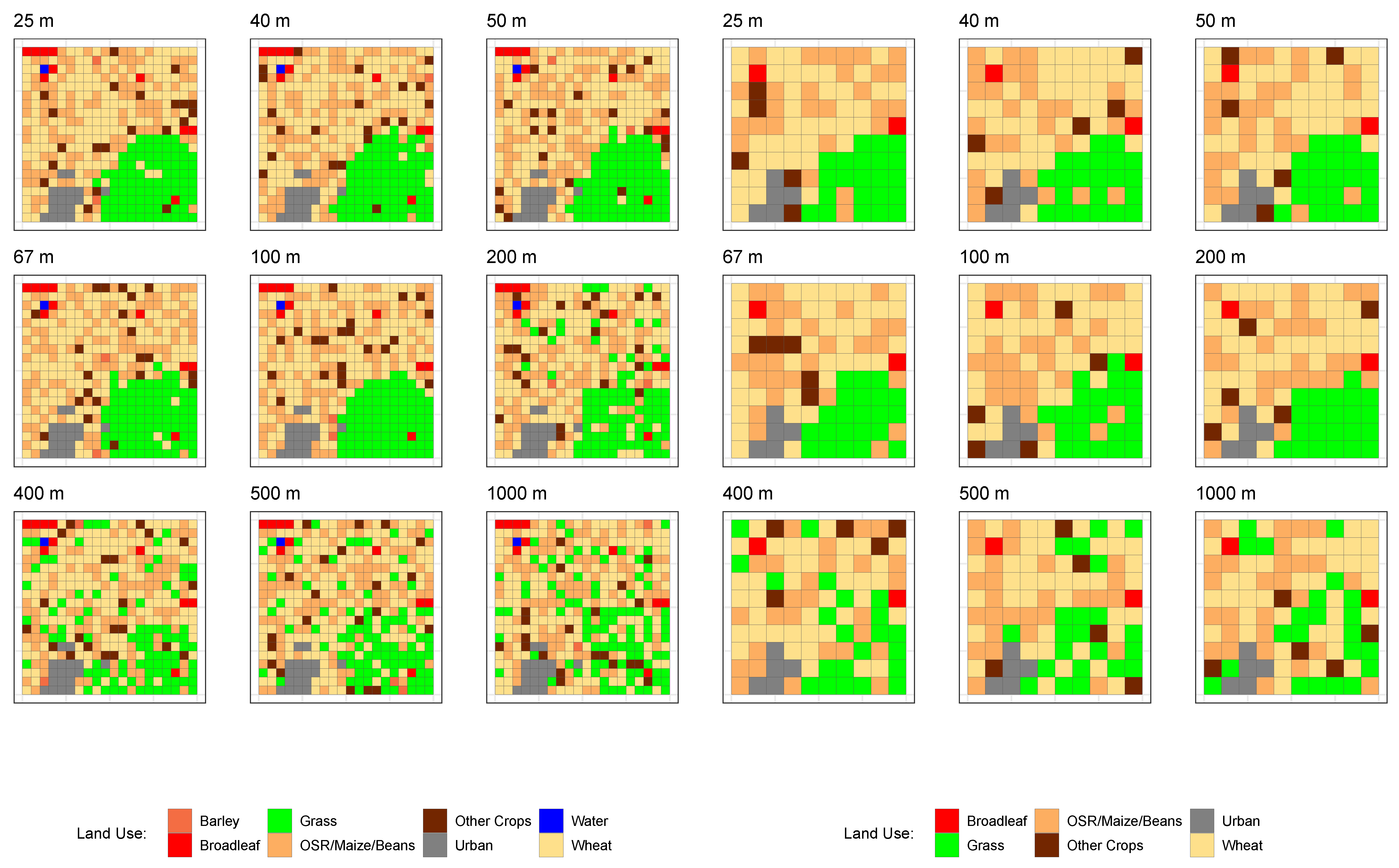
To evaluate the impacts of variations in scale, a series of land use optimisations was undertaken using the land use data in Figure 1 and aggregated to 40, 50, 67, 100, 200, 400, 500 and 1000 m resolutions, some of which are illustrated in Figure 2. These resolutions were chosen to illustrate a range of aggregation scales. The land use class for each grid cell was determined from the field data in Figure 1 using a spatial intersection in which the grid cell was labelled with the land use class with the greatest intersecting area. Notice how smaller land use parcels are excluded at coarser scales—the Barley and Water parcels at 200 m, for example.
In ES analyses, different land use types are conceptualised as supporting any given ES to differing degrees. In this study, ES scores were assigned to each land use class as in Table 2. These were derived from a local ES study [24] and are broadly related to some sort of regulating ES.
In order to examine the interactions of land use with ES, an ES gradient, , was also defined. This has greater intensity in the south and the east and uses a nonlinear decay function to create ES values:
where X and Y are the relative locations of each grid cell on a scale . The resulting ES gradient was aggregated over different scales, as shown in Figure 3. These surfaces could represent Provisioning, Regulating or Cultural ESs, such as Soil Fertility, Flood Risk or Wilderness, respectively.
3.2. Land Use Optimisation
The aims of the analyses described and undertaken below is to determine land use configurations that maximise ES provision to support some land use allocation decision and to examine how these are affected by data aggregation scales. In the allocation, the counts of the existing land use objects—the field parcels in Figure 1 or the grid cells or pixels in Figure 2—were retained, and the task is to identify the best set of locations for each land use object. This is a high dimensional search space: Each land use object can be allocated to each location, which in the case of the 200 m grid with 100 cells requires permutations to evaluate and in the case of the 100 m grid with 400 cells involving permutations.
A Genetic Grouping Algorithm (GGA) was used to explore this search space. GGAs were first proposed by [25] as an extension of classic Genetic Algorithms (GAs).
Optimisation with a GA first creates a set of potential solutions or chromosome, which are composed of genes, which in this case represents a set of specific locations (grid cells or fields) for specific land uses. The chromosomes or individual is then evaluated using some fitness criteria to assess the performance of the individual. Genes (locations) from successful individuals are interchanged in a crossover operation which combines two chromosomes to create new individuals, which are, in effect, offspring or children. To avoid stagnation, some gene mutation is introduced and, in this manner, the idea behind GAs is that they breed optimal solutions by creating and selecting fitter generations and, hence, the analogy with natural selection: Crossover creates new chromosomes from successful ones, and mutation ensures diversity. GGAs are a modification to classical GAs. They evaluate groups or subsets of individuals rather than only individuals and maintain group membership during the crossover operation for members that may have been displaced by other operations. GGAs have been found to be suited to location problems [26] due to the manner that GGAs approach the search space and the partitioning of potential solutions. Overviews of GGAs can be found in Comber et al. and Sasaki et al. [26,27], and comparisons of GAs and GGAs can be found in [28]. In this work, the algorithm described in Comber et al. and Sasaki et al. [26,27], itself based on the genalg R package [29], was further modified for land use allocation.
The key to any optimisation or search heuristic is the evaluation function. Here, this was to maximise the overall ES score. The reallocated land uses were evaluated by calculating the area weighted ES score using the land use specific scores in Table 2, the intersecting area weighted mean ES gradient values as in Figure 3 and the area of the field or grid cell as in Figure 1 and Figure 2. Thus, the objective was to maximise the following:
where i indexes the grid cells or fields G with allocated land use class, S is the ES score associated with land use as in Table 2, W is the underlying ES gradient value as in Figure 3 calculated from the area weighted mean of the intersection between the land use data (field or gridded) and ES gradients and A is the area of the field or grid cell in metres.
Land use reallocation analyses were undertaken using field (vector) data in Figure 1 and gridded (raster) data in Figure 2. In this case, no new land uses were introduced, rather, existing land use counts could be allocated to different fields or grid cells. In all analyses, a degree of elitism was used in which the top 30% of the current population was carried forward to the next and the probability of mutation was set at . Initial populations of the number of observations (fields as in Figure 1 or grid cells as in Figure 2) were created, from which the optimised set of land use reallocations was bred to allow the selection of a stronger population. The number of iterations was set to 3000 in each case, which was sufficient to ensure convergence for each reallocation. In each analysis, observations pertaining to Urban, Broadleaf and Water land uses were held in fixed locations and not reallocated as these classes cannot be easily transposed to another location.
The ES gradients in Figure 3 were used to optimise (re-allocate) the spatial distribution of land use using both the field data in Figure 1 and the gridded land use data in Figure 2. Thus, the analysis sought to optimise the field data and gridded land use data aggregated to 50, 67 100, 200, 400, 500 and 1000 m, with ES gradients at 25, 40 50, 67, 100, 200, 400, 500 and 1000 m.
Full details of the code, the data and functions used to undertake the analysis and to generate and map the results can be found at https://github.com/lexcomber/lu_maup/.
4. Results
4.1. Vector (Field) Land Use Data with Gridded ES Surfaces
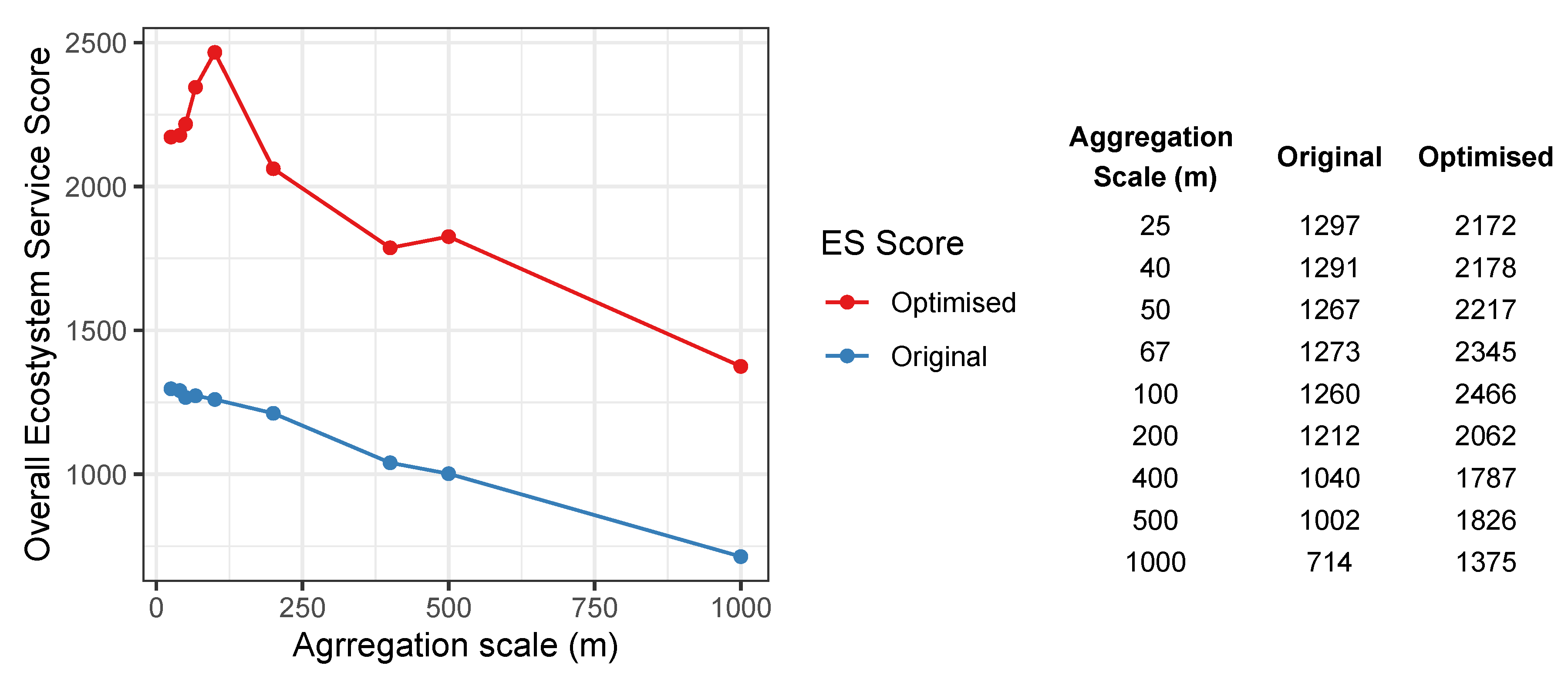
A series of optimisation analyses were undertaken that allocated land use in Figure 1 using ES aggregations illustrated in Figure 3. The original and optimised ES scores generated from ES gradients aggregated to different scales are shown in Figure 4 for field (vector) data. The original and optimised ES scores on the y axis are the sum of the land use scores in Table 2, multiplied by the area weighted mean of the intersecting ES gradients illustrated in Figure 3 and the area of the land use parcel, as in Equation (2). Optimised ES scores are consistently higher than the original ES scores.
Unsurprisingly, both original and optimised overall ES scores generally decline with increasing aggregation scale. This is because the information content and granularity of the ES gradient reduces as resolution increases. For example, the 400 m ES grid has 25 cells (see Figure 3), with a ES mean value of 2.44, compared to the 50 m grid with 1600 cells and an ES mean value of 2.69 and, in the extreme case, the 1000 m grid, with four cells with ES values of 0.05, 0.12, 1.84 and 5 and a mean ES value of 1.75. The result is that ES scores generated over gradients at coarser resolutions will necessarily result in coarser, less nuanced evaluations of ES, whether used for original land use configurations or optimised ones, regardless of whether the land use is in field (vector) format or gridded.
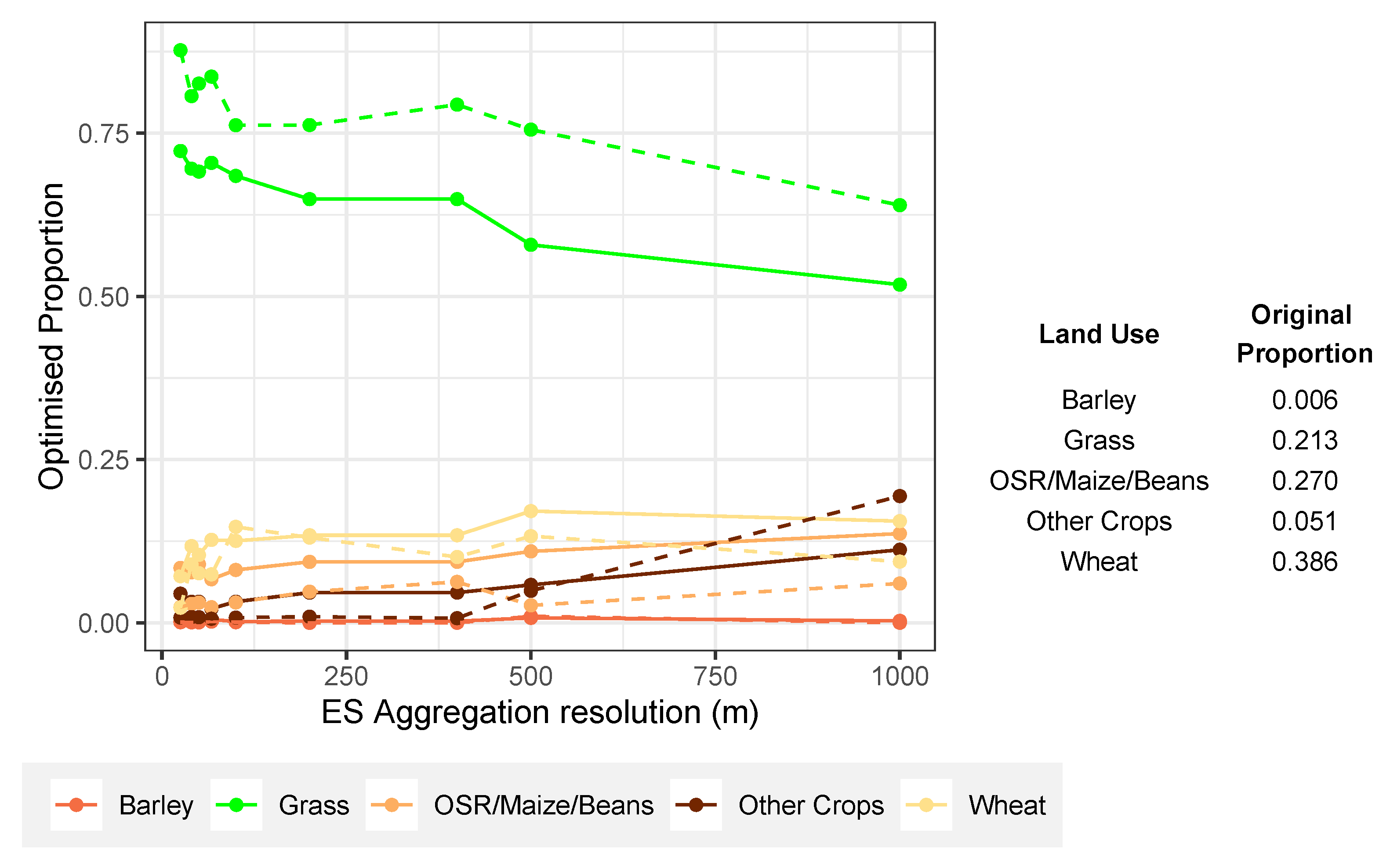
The second feature evident in Figure 4 is the distinct peak in the optimised ES scores when they are evaluated using the 100 m grid. This perfectly highlights aggregation effects associated with MAUP, for which its effects are frequently non-nested and non-hierarchical and intrinsically related to the scales of assessment and evaluation. It is possible to hypothesise that the peak in ES score at 100 m may be due to the combined impacts of land use reallocation driven by the aggregation of the ES gradient. To unpack this a bit more, Figure 5 shows the proportions of the case study area occupied by reallocated land use and the contribution of each land use class to the overall ES score. Here, the influence of reallocating the Grass class is evident, particularly at ES aggregation scales between 67 and 200 m. Of the arable related classes that were subject to reallocation (recall that Urban, Broadleaf, Water and Coniferous land uses were not reallocated), the Grass class has the highest degree of ES provision, and this is reflected in reallocation across scales, where essentially Grass replaces Wheat. Interestingly, the peak for Grass proportions is not at 100 m but at 25 m and the effect of the ES grid resolution can be seen in the decline in Grass proportions after 400 m and an associated increase in Wheat allocations.
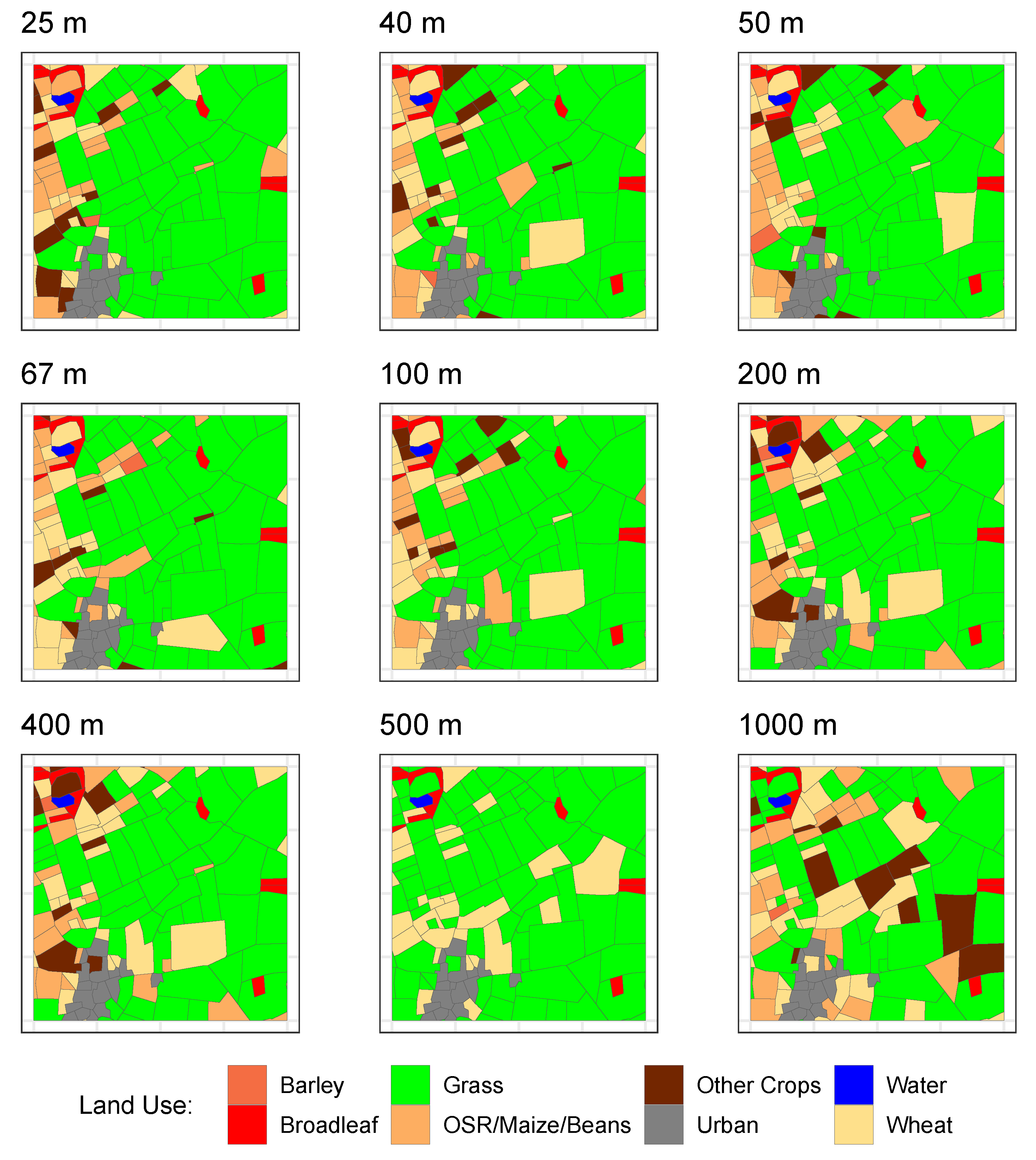
These scale effects are reflected in the different optimised land use configurations when undertaken using ES gradients at different scales (Figure 6). This also reflects the effects of MAUP: the aggregated ES gradients at coarser resolutions are not sufficiently granular to ’pull’ land uses with higher degrees of ES benefit towards the area to the south and east with high value areas of the ES gradient.
The results in Figure 4 and Figure 6 highlight the importance of understanding the influence of aggregation scales in the way that processes are represented in models and the need to match process with measurement scale. This is a key point. For example, agricultural land use data recorded for each field parcel have an inherent grain where the fundamental unit of analysis is the field parcel itself. The concept of granularity or grain in this context includes the inherent properties of objects, which in the case of a field includes the boundary (in the UK fields are commonly demarked by hedges, fences and or ditches), access via gates, etc.
4.2. Aggregated Land Use Data with Gridded ES Surfaces
A second set of land use optimisation analyses was undertaken by using aggregated land use data in Figure 2 and aggregated ES data in Figure 3. The aim here was to examine the effects of aggregation scale when analysing land use data in a regular gridded format, as is commonly the case in many ES and land cover/land use analyses. Evidently, there is some information loss with conversion from vector data in Figure 1, as each grid cell is allocated to a single land use class. However, many land use datasets and analyses adopt this ’pixel’ view of the world [30].
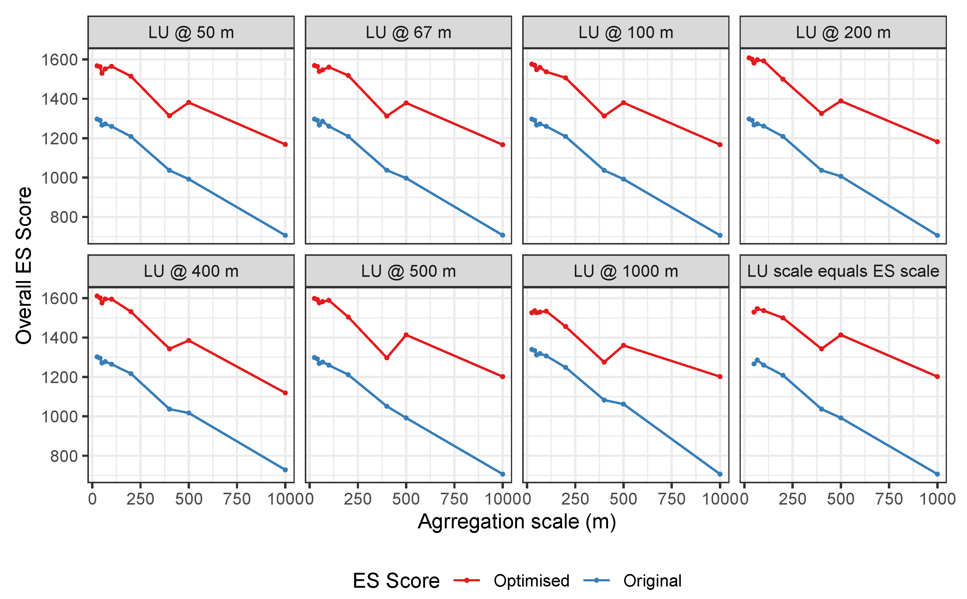
The optimisation scores using data aggregated to different scales are shown in Figure 7. Interestingly, the patterns are similar for each of the analyses:
- The ES score trends for the different scales of land use aggregation are similar under each ES gradient aggregation scale;
- The ES scores generally decline with increased ES gradient aggregation scale, for both the original and optimised allocations;
- These overall decreasing trends in ES score for optimised land use allocation are disturbed under the ES grids of 100 m and 500 m (sharp increase);
- These patterns are replicated when optimisation is undertaken using land use data and ES gradients are aggregated to the same spatial scales.
The results in Figure 7 strongly indicate that the variations in ES scores are generally being driven by ES aggregation rather than land use aggregations as similar trends are observed for each land use aggregation scale with ES aggregation as well as the trends in Figure 4. However, they also indicate the presence of scale related processes when ES gradients are aggregated to 100 m and 500 m that may be specific to this land use dataset and to these aggregation scales. These are also suggested in Figure 5. To investigate these, Figure 8 summarises the distributions of land use parcel perimeters (boundaries) and the square root of the parcel areas. It shows that the most frequent values in the distributions are land use parcels with an area of 10,000 m (1 ha) and a boundary of around 500 m. These indicate the origins of peak ES scores when ES gradients are aggregated to 100 m and 500 m in Figure 7, and thereby the impact of the specific spatial configuration of the field parcels on ES evaluations.
It is instructive to examine the allocated land use distributions. Figure 9 and Figure 10 show optimised land uses for the land use grids at 100, 200 and 500 m, using all nine of the ES gradients aggregated at different scales. The same trends as in Figure 7 are evident: the overall efficacy of the optimisation and the ES score both decreased as the ES gradient aggregation scale increased. This is because as ES granularity decreases (i.e., aggregation scale increases), they are increasingly unable to generate ES scores for land use objects that allow them to be reallocated, for example, by pulling the Grass land use objects (with high ES scores) towards the southeast corner of the study area (the region with high ES gradient values).
It important to recall what is being shown and what is being performed with the data. Land use data are at single aggregated scale, as shown by the grid cells in Figure 9 and Figure 10. The ES score for each object is generated from an area weighted mean of the intersection between the land use and the ES gradient. Thus, in Figure 10 there are 16 land use cells, for which its ES score is evaluated by 1600 ES gradient cells at 25 m (top left in Figure 10) but by four ES gradient cells at 1000 m (bottom right in Figure 10).
Consider the allocations in Figure 10 for the ES gradients aggregated to 25 m, 100 m and 500 m. These have the the same ES configurations but have different overall ES scores. They would have the same scores if they were evaluated over the same ES gradient, but they do not, as shown by the grid cell values in Figure 10. This illustrates the context of the better performance of land use allocations under the 500 m ES gradient in Figure 7 compared to 400 m; for example, it highlights the non-nested, non-hierarchical behaviours of scale under MAUP and the unpredictable nature of aggregation effects.
5. Discussion
The results of the case studies in this paper demonstrate the impacts of decision making on different scales of spatial aggregation and spatial support. The analyses reallocated land use in order to improve (optimise) the delivery of a single hypothetical ES over a small case study area. In this context, the land use reallocation and ES optimisation procedure illustrate issues associated with different scales of spatial support. A search heuristic (in this case a Grouping Genetic Algorithm) was used to optimise the spatial configurations of land use parcels in vector format and aggregated to grids of different resolutions. The land use reallocations and configurations were evaluated using an ES gradient aggregated over varying spatial supports and the GGA sought to maximise the overall ES score for the case study area. The aim of the analyses was to illustrate the effect of different scales of spatial support on decision making. For this reason, the case study was small and only a single ES was evaluated. In reality, ES evaluations were undertaken over larger scales (e.g., catchments) and considered multiple ES objectives (e.g., provisioning, cultural and regulating) and their interactions. To support such evaluations, ESs are commonly bundled [31,32] into groups of synergistic ESs, which co-vary to social and ecological pressures [33].
The results of this paper show first that, generally, as the scale of ES gradient aggregation increases (becomes coarser), the allocation evaluations are less effective due to the decreased resolving power and granularity of the ES gradient at increased aggregation scales. This overall trend was evident for land use in vector format (Figure 4) and grid formats (Figure 7) when reallocated using ES gradients aggregated to different scales to evaluate potential allocations.
A second feature of the reallocation results was that the overall trends of decreasing ES evaluation with increasing ES gradient aggregation were interrupted when the ES gradients were aggregated to 100 m and 500 m, as shown in Figure 4 and Figure 7 for vector and gridded land use. For this case study, the highest ES score results were generated under ES gradients aggregated to 100 m. There is the possibility that this non-hierarchical behaviour may be due to the arbitrary positioning of ES grids, although the same trends were observed in the analyses of both field (vector) and gridded land use data, suggesting that the agriculture-related processes in this study are best captured at that resolution.
Third, these trend discontinuities were shown to be due to the spatial interaction of the original land use data and the gridded ES gradients at these scales, as shown in Figure 8. This indicates that the “best” aggregation scale is driven by the spatial scale (support) of the underling case study data. It suggests that a different case study, containing field parcels with different typical spatial properties would be expected to show the same overall trends (of declining allocation effectiveness with increasing ES gradient aggregation) but with trend discontinuities at aggregation scales specific to case study data. However, this has not been substantiated in this study and suggests an area for further investigation.
Together, these results clearly indicate how decisions around land allocation and ES, whether at the field, grid, catchment or landscape scale, are mediated by the spatial support of data. The effects of the spatial support were shown to be nonlinear, non-nested and non-hierarchical and sensitive to the spatial properties and grain of the underlying objects (e.g., agricultural fields) and the data used to represent them in ES analyses (as shown in the trends in Figure 4 and Figure 7). In turn, this makes the impacts of scale difficult to predict. It indicates that the evaluations of process spatial scale (in this case land use) should be undertaken at different scales of aggregation as part of any ES analyses and evaluation.
Extending this further, this also suggests that land use evaluations may benefit from locally varying scales of aggregation to reflect the spatial variation in the processes that are examined—in this case, land use. Figure 11 shows a quadtree representation of the data in Figure 1, suggesting how scales of aggregation could be locally determined to reflect locally varying spatial proprieties of the objects being evaluated. However, this is very much an area for further research.
6. Conclusions
There are a number of recommendations arising from this work for research that incorporates analyses of land use, ES and NC evaluations:
- MAUP should always be tested for. Any analysis of spatial data should routinely test for MAUP in order to understand the specific impacts of aggregations scales relative to the spatial support of the process being investigated. This is a common consideration in socio-economic analyses of spatial data [1] but has yet to be adopted in the ES domain and in work seeking to evaluate NC and to inform landscape decisions, land use planning and ES delivery.
- The scale of spatial data aggregations should be matched to the granularity of the processes being evaluated. This requires the identification of spatial scales at which the processes being investigated are considered to be stationary (stable) with respect to their variances, covariances and other moments in order to ensure that the results of any analyses, such as land use allocation in this study, are not affected by inherent scale mismatches. Here, these were observed under ES gradients aggregated to scales other than 100 and 500 m and can be determined by using local indicators of spatial association [34,35] or local spatial covariances [36].
- The impact of MAUP and aggregation scales should be evaluated alongside the scale of decision making. The support size and shape of the spatial units being used in spatial data analysis affect the patterns identified in the evaluations of ES and related concepts such as NC for a given spatial extent such as an agricultural field, a farm holding or river catchment.
- ES researchers and those in related disciplines (land use planning, landscape-scale decisions, etc.) should up-skill themselves in spatial analysis techniques. It is important that those undertaking research in these domains understand core paradigms associated with working with spatial data and understand techniques that are frequently used in spatial statistics. Scale blindness is commonly found in published ES research (as indicated above), where, for example, models constructed over one scale of spatial support are applied to data over another. Up-skilling is needed because powerful analytical tools that were previously the reserve of domain experts are now included in many off-the-shelf software environments and are easily applied in a naive manner. Such tools include those for spatial data aggregation (both up and down scaling), location allocation and spatial data integration. They will generate results without requiring the user to understand how to best parameterise them. Examples of similar misuse have been observed in the renewable energy literature with respect to land use [37].
The dangers of not undertaking such investigations into these MAUP and scale related considerations are erroneous inference and decision making. In the realm of ES and landscape decision making, there is a need to examine cross-scale sensitivities driven by the size and shape of areal units, as these relate to the scale component and aggregation or zoning component of the MAUP, respectively. Such investigations are needed to explicitly mitigate MAUP and to better handle different scales of decision making and response in models and decision tools. To perform this, there is a need to transfer and adapt concepts and methods from (i) Geostatistics [38,39], (ii) Spatial Ecology [35] and (iii) Quantitative Geography [40,41]. MAUP can be mitigated against by analysing data at the finest possible meaningful scale or unit [42]. Here, Geostatistics provides predictive tools to down-scale with an associated variance [43] and statistical tests of sensitivity relative to MAUP can inform on this ideal scale [44].
However, a ‘solution’ to the MAUP poses a very different challenge: spatial scales need to be identified where the study processes are considered stable with respect to their variances, covariances and higher moments in context of the intended data analysis. Such local scale stability has strong links to the notion of process non-stationarity, where investigations, for example, by using local indicators of spatial association [34,35] or local spatial covariances (variograms) [36] have the potential to provide ‘solutions’ to MAUP.
Author Contributions
Conceptualization, A.C. and P.H.; methodology, A.C.; software, A.C.; formal analysis, A.C.; writing—original draft preparation, A.C; writing—review and editing, A.C. and P.H. All authors have read and agreed to the published version of the manuscript.
Funding
This research was funded by UK Natural Environment Research Council grant numbers NE/S009124/1 (A.C.) and NE/N007433/1 (P.H.). The APC was funded by UK Natural Environment Research Council.
Institutional Review Board Statement
Not applicable.
Informed Consent Statement
Not applicable.
Data Availability Statement
The code and data used in this analysis are available from https://github.com/lexcomber/lu_maup/.
Acknowledgments
The authors would like to acknowledge the following data sources: CEH Land Cover® Plus: Crops 2018 © NERC (CEH) 2018. © RSAC. © Crown Copyright 2007, Licence number 10001757; Land Cover Map 2015 [FileGeoDatabase geospatial data], Scale 1:2500, Tiles: GB, Updated: 26 May 2017, CEH, Using: EDINA Environment Digimap Service, https://0-digimap-edina-ac-uk<.brum.beds.ac.uk/a>, Downloaded: 2019-04-26 14:47:27.28; Land Cover plus: Crops (2018) [GeoPackage geospatial data], Scale 1:2500, Tiles: GB, Updated: 4 December 2018, CEH, Using: EDINA Environment Digimap Service, https://0-digimap-edina-ac-uk<.brum.beds.ac.uk/a>, Downloaded: 2019-04-26 15:16:52.69. We thank the anonymous reviewers of this manuscript whose comments and suggestions considerably improved the paper.
Conflicts of Interest
The authors declare no conflict of interest. The funders had no role in the design of the study; in the collection, analyses or interpretation of data; in the writing of the manuscript; or in the decision to publish the results.
References
- Brunsdon, C.; Comber, A. Opening practice: Supporting reproducibility and critical spatial data science. J. Geogr. Syst. 2021, 23, 477–496. [Google Scholar] [CrossRef]
- Spake, R.; Bellamy, C.; Gill, R.; Watts, K.; Wilson, T.; Ditchburn, B.; Eigenbrod, F. Forest damage by deer depends on cross-scale interactions between climate, deer density and landscape structure. J. Appl. Ecol. 2020, 57, 1376–1390. [Google Scholar] [CrossRef]
- Finch, T.; Day, B.H.; Massimino, D.; Redhead, J.W.; Field, R.H.; Balmford, A.; Green, R.E.; Peach, W.J. Evaluating spatially explicit sharing-sparing scenarios for multiple environmental outcomes. J. Appl. Ecol. 2021, 58, 655–666. [Google Scholar] [CrossRef]
- Openshaw, S. The Modifiable Areal Unit Problem, CATMOG 38; Geo Abstracts: Norwich, UK, 1984. [Google Scholar]
- Openshaw, S. Ecological fallacies and the analysis of areal census data. Environ. Plan. A 1984, 16, 17–31. [Google Scholar] [CrossRef] [Green Version]
- Dungan, J.L.; Perry, J.; Dale, M.; Legendre, P.; Citron-Pousty, S.; Fortin, M.J.; Jakomulska, A.; Miriti, M.; Rosenberg, M. A balanced view of scale in spatial statistical analysis. Ecography 2002, 25, 626–640. [Google Scholar] [CrossRef] [Green Version]
- Grêt-Regamey, A.; Weibel, B.; Bagstad, K.J.; Ferrari, M.; Geneletti, D.; Klug, H.; Schirpke, U.; Tappeiner, U. On the effects of scale for ecosystem services mapping. PLoS ONE 2014, 9, e112601. [Google Scholar] [CrossRef]
- Atkinson, P.M.; Graham, A. Issues of scale and uncertainty in the global remote sensing of disease. Adv. Parasitol. 2006, 62, 79–118. [Google Scholar]
- Comber, A.J.; Harris, P.; Lü, Y.; Wu, L.; Atkinson, P.M. The Forgotten Semantics of Regression Modeling in Geography. Geogr. Anal. 2021, 53, 113–134. [Google Scholar] [CrossRef] [Green Version]
- Jones, K.; Manley, D.; Johnston, R.; Owen, D. Modelling residential segregation as unevenness and clustering: A multilevel modelling approach incorporating spatial dependence and tackling the MAUP. Environ. Plan. Urban Anal. City Sci. 2018, 45, 1122–1141. [Google Scholar] [CrossRef] [Green Version]
- Arbia, G.; Espa, G. Effects of the MAUP on image classification. Geogr. Syst. 1996, 3, 123–141. [Google Scholar]
- Gotway, C.A.; Young, L.J. Combining incompatible spatial data. J. Am. Stat. Assoc. 2002, 97, 632–648. [Google Scholar] [CrossRef] [Green Version]
- Zhang, J.; Atkinson, P.; Goodchild, M.F. Scale in Spatial Information and Analysis; CRC Press: Boca Raton, FL, USA, 2014. [Google Scholar]
- Murakami, D.; Tsutsumi, M. Area-to-point parameter estimation with geographically weighted regression. J. Geogr. Syst. 2015, 17, 207–225. [Google Scholar] [CrossRef] [Green Version]
- Fotheringham, A.S.; Wong, D.W. The modifiable areal unit problem in multivariate statistical analysis. Environ. Plan. A 1991, 23, 1025–1044. [Google Scholar] [CrossRef]
- Navas, A.L.A.; Osei, F.; Magalhães, R.J.S.; Leonardo, L.R.; Stein, A. Modelling the impact of MAUP on environmental drivers for Schistosoma japonicum prevalence. Parasites Vectors 2020, 13, 1–18. [Google Scholar]
- Zen, M.; Candiago, S.; Schirpke, U.; Vigl, L.E.; Giupponi, C. Upscaling ecosystem service maps to administrative levels: Beyond scale mismatches. Sci. Total Environ. 2019, 660, 1565–1575. [Google Scholar] [CrossRef]
- Frazier, A.E.; Kedron, P. Landscape metrics: Past progress and future directions. Curr. Landsc. Ecol. Rep. 2017, 2, 63–72. [Google Scholar] [CrossRef] [Green Version]
- Hellsten, S. A Spatio-Temporal Ammonia Emissions Inventory for the UK. Ph.D. Thesis, University of Edinburgh, Edinburgh, UK, 2006. [Google Scholar]
- Harper, A.B.; Powell, T.; Cox, P.M.; House, J.; Huntingford, C.; Lenton, T.M.; Sitch, S.; Burke, E.; Chadburn, S.E.; Collins, W.J.; et al. Land-use emissions play a critical role in land-based mitigation for Paris climate targets. Nat. Commun. 2018, 9, 2938. [Google Scholar] [CrossRef] [Green Version]
- Rowland, C.; Morton, D.; Carrasco Tornero, L.; McShane, G.; O’Neil, A.; Wood, C. Land Cover Map 2015 (Vector, GB); NERC Environmental Information Data Centre: Gwynedd, UK, 2017. [Google Scholar] [CrossRef]
- Rowland, C.; Morton, D.; Carrasco Tornero, L.; McShane, G.; O’Neil, A.; Wood, C. Land Cover Map 2015 (25 m Raster, GB); NERC Environmental Information Data Centre: Gwynedd, UK, 2017. [Google Scholar] [CrossRef]
- Rowland, C.; Morton, D.; Carrasco Tornero, L.; McShane, G.; O’Neil, A.; Wood, C. Land Cover Map 2015 (1 km Dominant Target Class, GB); NERC Environmental Information Data Centre: Gwynedd, UK, 2017. [Google Scholar] [CrossRef]
- Smith, A.; Dunford, R. Land-Cover Scores for Ecosystem Service Assessment. 2018. Available online: https://www.eci.ox.ac.uk/research/ecosystems/bio-clim-adaptation/downloads/bicester-2018-Land-cover-scoring-method%20.pdf (accessed on 26 April 2019).
- Falkenauer, E. Genetic Algorithms and Grouping Problems; John Wiley & Sons Inc.: Hoboken, NJ, USA, 1998. [Google Scholar]
- Comber, A.J.; Sasaki, S.; Suzuki, H.; Brunsdon, C. A modified grouping genetic algorithm to select ambulance site locations. Int. J. Geogr. Inf. Sci. 2011, 25, 807–823. [Google Scholar] [CrossRef] [Green Version]
- Sasaki, S.; Comber, A.J.; Suzuki, H.; Brunsdon, C. Using genetic algorithms to optimise current and future health planning-the example of ambulance locations. Int. J. Health Geogr. 2010, 9, 4. [Google Scholar] [CrossRef] [Green Version]
- Brown, E.C.; Sumichrast, R.T. Evaluating performance advantages of grouping genetic algorithms. Eng. Appl. Artif. Intell. 2005, 18, 1–12. [Google Scholar] [CrossRef]
- Willighagen, E. R Based Genetic Algorithm, R Package Version 2005; p. 1. Available online: https://cran.r-project.org/web/packages/genalg/index.html (accessed on 26 April 2019).
- Fisher, P. The pixel: A snare and a delusion. Int. J. Remote Sens. 1997, 18, 679–685. [Google Scholar] [CrossRef]
- Raudsepp-Hearne, C.; Peterson, G.D.; Bennett, E.M. Ecosystem service bundles for analyzing tradeoffs in diverse landscapes. Proc. Natl. Acad. Sci. USA 2010, 107, 5242–5247. [Google Scholar] [CrossRef] [PubMed] [Green Version]
- Mouchet, M.A.; Lamarque, P.; Martín-López, B.; Crouzat, E.; Gos, P.; Byczek, C.; Lavorel, S. An interdisciplinary methodological guide for quantifying associations between ecosystem services. Glob. Environ. Chang. 2014, 28, 298–308. [Google Scholar] [CrossRef]
- Spake, R.; Lasseur, R.; Crouzat, E.; Bullock, J.M.; Lavorel, S.; Parks, K.E.; Schaafsma, M.; Bennett, E.M.; Maes, J.; Mulligan, M.; et al. Unpacking ecosystem service bundles: Towards predictive mapping of synergies and trade-offs between ecosystem services. Glob. Environ. Chang. 2017, 47, 37–50. [Google Scholar] [CrossRef] [Green Version]
- Anselin, L. Local indicators of spatial association—LISA. Geogr. Anal. 1995, 27, 93–115. [Google Scholar] [CrossRef]
- Hui, C. A Bayesian solution to the modifiable areal unit problem. In Foundations of Computational Intelligence; Springer: Berlin/Heidelberg, Germany, 2009; Volume 2, pp. 175–196. [Google Scholar]
- Harris, P.; Charlton, M.; Fotheringham, A.S. Moving window kriging with geographically weighted variograms. Stoch. Environ. Res. Risk Assess. 2010, 24, 1193–1209. [Google Scholar] [CrossRef] [Green Version]
- Comber, A.; Dickie, J.; Jarvis, C.; Phillips, M.; Tansey, K. Locating bioenergy facilities using a modified GIS-based location–allocation-algorithm: Considering the spatial distribution of resource supply. Appl. Energy 2015, 154, 309–316. [Google Scholar] [CrossRef] [Green Version]
- Cressie, N.A. Change of support and the modifiable areal unit problem. Geogr. Syst. 1996, 3, 159–180. [Google Scholar]
- Young, L.J.; Gotway, C.A. Linking spatial data from different sources: The effects of change of support. Stoch. Environ. Res. Risk Assess. 2007, 21, 589–600. [Google Scholar] [CrossRef]
- Dark, S.J.; Bram, D. The modifiable areal unit problem (MAUP) in physical geography. Prog. Phys. Geogr. 2007, 31, 471–479. [Google Scholar] [CrossRef] [Green Version]
- Parenteau, M.P.; Sawada, M.C. The modifiable areal unit problem (MAUP) in the relationship between exposure to NO2 and respiratory health. Int. J. Health Geogr. 2011, 10, 58. [Google Scholar] [CrossRef] [PubMed] [Green Version]
- Tuson, M.; Yap, M.; Kok, M.; Murray, K.; Turlach, B.; Whyatt, D. Incorporating geography into a new generalized theoretical and statistical framework addressing the modifiable areal unit problem. Int. J. Health Geogr. 2019, 18, 6. [Google Scholar] [CrossRef] [PubMed] [Green Version]
- Kyriakidis, P.C. A geostatistical framework for area-to-point spatial interpolation. Geogr. Anal. 2004, 36, 259–289. [Google Scholar] [CrossRef]
- Duque, J.C.; Laniado, H.; Polo, A. S-maup: Statistical test to measure the sensitivity to the modifiable areal unit problem. PLoS ONE 2018, 13, e0207377. [Google Scholar] [CrossRef]
Figure 1.
The land use data projected to OSGB 1936 (CRS 27700).

Figure 2.
Examples of the land use data aggregated to different scales.

Figure 3.
Examples of an ecosystem service gradient aggregated to different scales.

Figure 4.
Examples of an Ecosystem Service gradient aggregated at different scales.

Figure 5.
The proportions of different land use classes in the study area (solid line) and the proportion of the total ES score associated with each land use (dashed line) when optimised using an ES gradient aggregated to different resolutions.
Figure 5.
The proportions of different land use classes in the study area (solid line) and the proportion of the total ES score associated with each land use (dashed line) when optimised using an ES gradient aggregated to different resolutions.

Figure 6.
The land use allocations arising from ES gradients aggregated to different scales.

Figure 7.
The original and optimised ecosystem service scores (y-axis) of the gridded land use data, evaluated over different ES gradients (x-axis) aggregated over different scales.
Figure 7.
The original and optimised ecosystem service scores (y-axis) of the gridded land use data, evaluated over different ES gradients (x-axis) aggregated over different scales.

Figure 8.
Histograms of the square root of area and boundary length of the original land use parcels.
Figure 8.
Histograms of the square root of area and boundary length of the original land use parcels.

Figure 9.
Optimised land use allocations for the 100 m land use grid (right hand side) and 200 m land use grid (left hand side) under different scales of ES gradient aggregation.
Figure 9.
Optimised land use allocations for the 100 m land use grid (right hand side) and 200 m land use grid (left hand side) under different scales of ES gradient aggregation.

Figure 10.
Optimised land use allocations for the 500 m land use grid under different scales of ES gradient aggregation. The cell values are the land use grid cell ES scores that are summed to generate the overall ES score.
Figure 10.
Optimised land use allocations for the 500 m land use grid under different scales of ES gradient aggregation. The cell values are the land use grid cell ES scores that are summed to generate the overall ES score.

Figure 11.
A simple quadtree representation of the parcel data, indicating the spatial variation and distribution of potentially ’appropriate’ scales of aggregation (grid cell dimensions).
Figure 11.
A simple quadtree representation of the parcel data, indicating the spatial variation and distribution of potentially ’appropriate’ scales of aggregation (grid cell dimensions).


Table 1.
The look-up table used to reclassify land cover and crop data.
| Original Classes | New Label |
|---|---|
| Spring barley, Winter barley | Barley |
| Broadleaf woodland | Broadleaf |
| Coniferous woodland | Coniferous |
| Grass, Improved grassland | Grass |
| Neutral grassland | Natural Grass |
| Field beans, Maize, Oilseed rape | OSR/Maize/Beans |
| Arable and horticulture, pother crops, Potatoes | Other Crops |
| Suburban, Urban | Urban |
| Freshwater | Water |
| Spring Wheat, Winter wheat (includes winter oats) | Wheat |
Table 2.
The degree of Ecosystem Service provided by each land use class.
| Land Use | ES Score |
|---|---|
| Barley | 1 |
| Broadleaf | 5 |
| Grass | 2 |
| Natural Grass | 3 |
| OSR/Maize/Beans | 1 |
| Other Crops | 1 |
| Urban | 1 |
| Water | 3 |
| Wheat | 1 |
Publisher’s Note: MDPI stays neutral with regard to jurisdictional claims in published maps and institutional affiliations. |
© 2022 by the authors. Licensee MDPI, Basel, Switzerland. This article is an open access article distributed under the terms and conditions of the Creative Commons Attribution (CC BY) license (https://creativecommons.org/licenses/by/4.0/).
Share and Cite
MDPI and ACS Style
Comber, A.; Harris, P. The Importance of Scale and the MAUP for Robust Ecosystem Service Evaluations and Landscape Decisions. Land 2022, 11, 399. https://0-doi-org.brum.beds.ac.uk/10.3390/land11030399
AMA Style
Comber A, Harris P. The Importance of Scale and the MAUP for Robust Ecosystem Service Evaluations and Landscape Decisions. Land. 2022; 11(3):399. https://0-doi-org.brum.beds.ac.uk/10.3390/land11030399
Chicago/Turabian StyleComber, Alexis, and Paul Harris. 2022. "The Importance of Scale and the MAUP for Robust Ecosystem Service Evaluations and Landscape Decisions" Land 11, no. 3: 399. https://0-doi-org.brum.beds.ac.uk/10.3390/land11030399
Note that from the first issue of 2016, this journal uses article numbers instead of page numbers. See further details here.