
Optimization of Production–Living–Ecological Space in National Key Poverty-Stricken City of Southwest China


1
School of Management, Tianjin University of Commerce, Tianjin 300131, China
2
Institute of Geographic Sciences and Natural Resources Research, Chinese Academy of Sciences, Beijing 100101, China
3
College of Resources and Environment, University of Chinese Academy of Sciences, Beijing 100049, China
4
Key Laboratory of Carrying Capacity Assessment for Resource and Environment, Ministry of Land & Resources, Beijing 100101, China
*
Author to whom correspondence should be addressed.
Land 2022, 11(3), 411; https://0-doi-org.brum.beds.ac.uk/10.3390/land11030411
Submission received: 28 February 2022
/
Revised: 7 March 2022
/
Accepted: 9 March 2022
/
Published: 11 March 2022
(This article belongs to the Special Issue Land Use Conflict Detection and Multi-Objective Optimization Based on the Productivity, Sustainability, and Livability Perspective)
Abstract
:Trade-offs and conflicts among different sectors of production, living, and ecology have become important issues in regional sustainable development planning due to both the versatility and limitation of land resources, especially in poverty-stricken mountainous areas. This study builds an optimization model to assist policymakers in simulating land demand and allocation in the future. The model takes socioeconomic and demographic development into consideration and couples local planning policy with land use data from the perspective of system integration. The model was employed for a case study of Zhaotong city to optimize production–living–ecological (PLE) space. The results show that the model provides a feasible method to explore the sustainable development pattern of territorial space, especially in distressed regions.
1. Introduction
Interactions between human and the environment have attracted increasing attention [1]. In general, cross-sectoral issues involve a variety of social and natural knowledge [2]. Gaps between natural and social sciences imply that understanding the mechanisms underlying human–environment systems from a systematic perspective is crucial to sustainable development [3]. To a certain extent, several studies have reflected the fact that the problems are multi-scale and complex while the solutions are diverse [4,5]. Effective domestic policymaking hinges on diverse stakeholders, which plays a critical role in accelerating the localization of the SDGs (Sustainable Development Goals, proposed by the United Nations in 2015) [6]. National development plans for the 2030 Agenda in many countries try to position human, social, environmental, economic, and institutional objectives at the same level [7,8,9]. However, a scientific challenge that obviously exists in sustainable issues is trade-offs and compensation. The achievement of one SDG is often at the cost of sacrificing or assisting another [10,11,12,13].
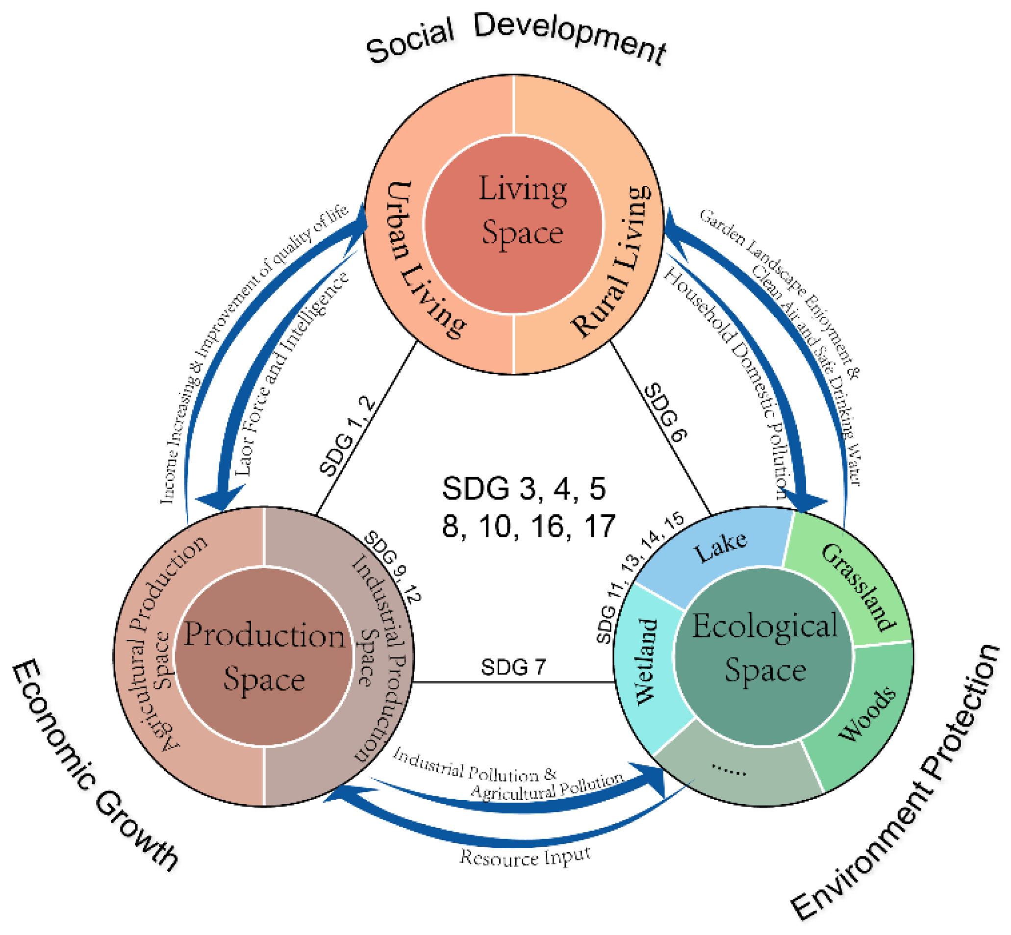
By 2020, China achieved the goal of eliminating poverty, which was accompanied by economic growth and rapid urbanization and contributed to SDG 1 [14,15]. Unfortunately, inconsistent and rough terrestrial land development patterns in production space and living space have placed pressure on ecological protection and resource security for ecological spaces [16,17,18,19]. To control the intensity of terrestrial land development and adjust the spatial structure, the concept of PLE (production–living–ecology) space was proposed in the report of the 18th National Congress of the Communist Party of China. The objective is to construct intensive and efficient production space, livable and appropriate living space, and protected and beautiful ecological space with beautiful mountains and clear water based on the principle of balancing economic, social, and ecological benefits. It aims to delimit the boundaries of multi-function terrestrial land development and establish a system for future sustainable land development [20]. To a certain extent, PLE space can be considered a combination of SDG indicators from a land function point of view (Figure 1). It is highly relevant to the 17 SDGs that involve environmental integrity, social equity, and economic prosperity, which comprise the triple bottom line approach of human wellbeing [21,22].
International academic research has discussed food security [23], tourism [24], agriculture [25], and urban regeneration [26] under the background of urban sustainability but rarely focuses on PLE space. After all, the concept has been proposed by the Chinese government in the context of China. Most studies are conducted on a domestic scope. Huang et al. claimed that the assessment of regional spatial carrying capacity and suitability is an important guideline for PLE space optimization [20]. Wu et al. indicated that the carrying capacity determines the upper limit of the PLE space in quantity, while suitability evaluation is related to the spatial layout structure [27]. Some studies have provided qualitative and empirical optimization suggestions based on the results of the carrying capacity and suitability evaluation [28,29,30]. In general, the suggestions point out that rules and regulations should be further enhanced and technology standards need to be improved in the future. However, it is uncertain whether these suggestions are feasible and effective. It is necessary to develop quantified and visualized tools to simulate future scenarios, especially for policymakers who face the difficulty of applying social and ecological approaches to decision-making [31].
Land resources are the most constrained factor for PLE space optimization. One parcel of land may be used as production space or as living space. In addition, land policy has become an indispensable means of macroeconomic regulation under China’s national policies because land resources have both natural and economic properties. Therefore, some studies approach PLE space optimization as a mathematical problem of multi-objective optimization, guiding maximum economic benefits, social benefits, and ecological benefits [32]. However, two major gaps remain in the literature. Firstly, multi-objective optimization algorithms still face some challenges in flexibility and convergence, especially in preference adaptation for various formulations [33,34]. Secondly, difficulty and complexity increase when referencing spatial data, although addressing quantitative issues has significant advantages.
The system dynamics model seeks opportunities and ways to optimize the structure of the system from a holistic perspective based on the feedback characteristics of the internal components [35,36,37]. It fills the first gap presented above. In contrast to multi-objective optimization equations, the system dynamics model simulates the real world by establishing relationships between social and economic factors. This method can introduce more factors and equations and perform dynamic simulations. SD models have been used in resource management, such as future urbanization and water scarcity [16], energy consumption [38], and water resource management systems [39]. However, the ability of the SD model to be applied in spatial allocation is very weak.
As for the other gap, the FLUS (Future Land Use Simulation) model (https://geosimulation.cn/FLUS.html, accessed on 15 February 2022) is used to simulate human activities and natural influences on land-use change and future scenarios. The model introduces an artificial neural network algorithm (ANN)-based probability calculation of suitability for various land use types based on traditional meta-automata. It proposes an adaptive inertial competition mechanism based on roulette selection (a stochastic selection method) [40], which can effectively deal with the uncertainty and complexity of multiple land-use types when they are transformed under the joint influence of natural effects and human activities, meaning the FLUS model has high simulation accuracy and can obtain similar results to the real land-use distribution [41]. To date, the model has been successfully applied in many cases, such as the simulation of future urban sprawl boundaries [42,43] and the simulation of flooding risks in rapid urbanization [44]. Furthermore, the input of future demand for land in the FLUS model can be determined by SD models, which means that the two can be well coupled. Sustainable development issues require a systematic approach to integrate various socioeconomic and environmental components that interact across regional levels, space, and time [45]. Some studies have integrated the idea of system science into the optimization of resource allocation [46,47,48] but rarely have focused on PLE space optimization. This paper aims to build an optimization model based on the SD and FLUS models, in which PLE space can be planned quantitatively and spatially under future scenarios.
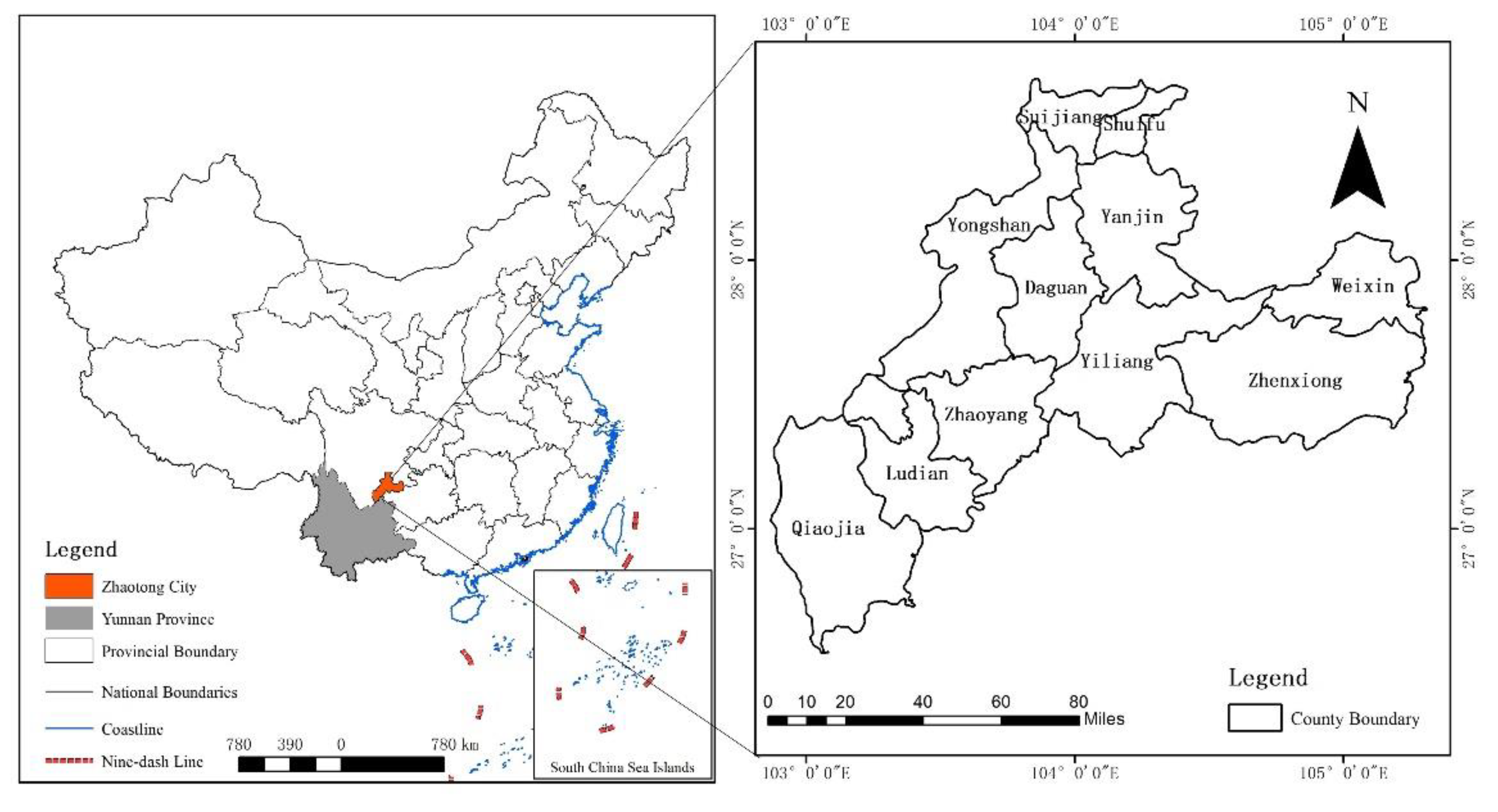
Trade-offs and conflicts of the PLE function are more obvious and intense in the poor areas of southwest China. Yunnan Province has the highest number of poverty-stricken counties and includes Zhaotong city, which is located in Wumeng Mountain and was one of the 14 concentrated contiguous poverty-stricken areas in China until 2020 (Figure 2). The GDP per capita is far below the national average level. People’s living standards and social development are limited by natural geographical conditions and ecosystem protection [49,50]. It is necessary to balance development and conservation when making future policies [51]. This paper has two main tasks, one is to develop a model applicable to the problem, and the other is to use the model to provide solutions for the future development of Zhaotong city, and attempt to answer the following questions: (1) In this impoverished region, what is the main trend in PLE space changes over the past few years? (2) Which scenario can meet the planning target of 2030? (3) How can the development pattern be optimized?
2. Methods and Data
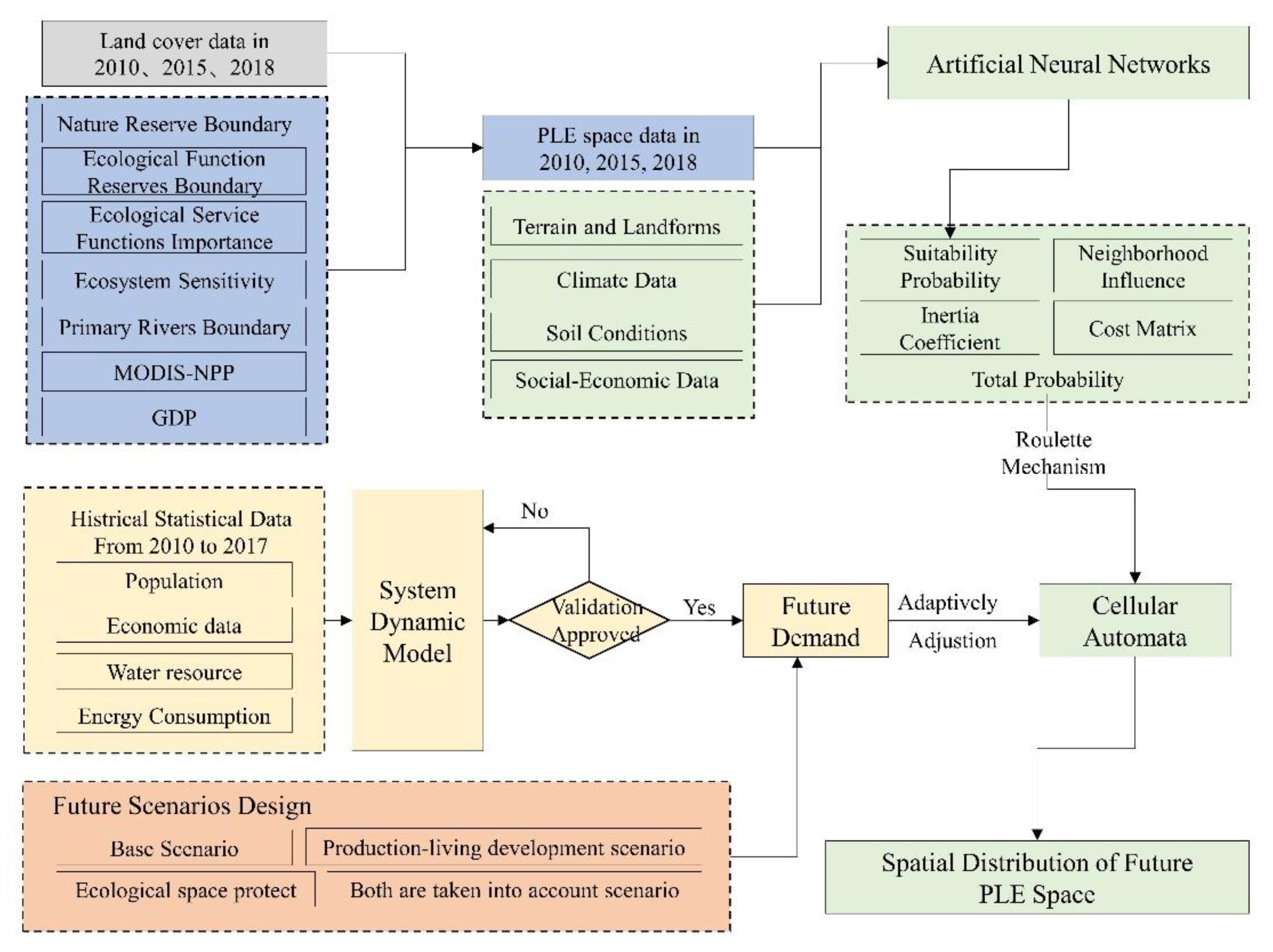
This paper aims to build an optimization model based on system dynamics and FLUS in which land resources can be planned quantitatively and spatially in terms of PLE space. A system dynamics model is employed to simulate the structure of the PLE space system and predict quantitative demand in 2030. FLUS is applied to allocate the land parcels at the spatial scale. The workflow is shown in Figure 3. The work consists of 4 main parts:
- (1)
- Classification of PLE space. PLE space is divided into production, living, and ecological space based on land-use data. Then, space is further divided into subclasses according to the function assessment, which serves as the basis for the subsequent PLE space optimization.
- (2)
- Establishment of the SD Model. We simulate the demand quantity of each PLE space and piece of land in 2030 by constructing a dynamic system model of PLE space, including the population, economy, and land system.
- (3)
- FLUS Model Settings. We take the quantity of demand obtained by (2) as the input data of the FLUS model and carry out spatial allocation of various PLE classes.
- (4)
- Constrained scenario design and analysis. Based on verifying the accuracy of the models in (2) and (3), a variety of future optimization scenarios are designed for simulation, and the simulation results are evaluated from multiple perspectives.
2.1. Classification of PLE Space
The classification of PLE space is the basis for the optimization of space layout. For PLE space optimization, it is necessary to clarify the priority. This study proposes a new classification system. According to the production–living–ecological function, the first level of classification was carried out, and then the second category was determined based on the land-use data from 2010, 2015, and 2018.
2.1.1. Detailed Data Sources
Based on the dataset of the multiperiod land cover dataset of China (MLC), the classification system of the “PLE space” is established. Detailed data sources are shown in Table 1. The MLC dataset was obtained by manual visual interpretation using Landsat remote sensing image data from the US. The land-use types include the six primary types of cropland, forestland, grassland, water, residential land, and unused land, and 25 secondary types. All raster datasets were resampled to 30 m by software Arcgis 10.2. As shown in Table 1, some datasets that are shared online publicly are limited due to temporal resolution.
2.1.2. Classification System
As shown in Table 2, according to the importance of ecological functions, ecological space is further subdivided into four secondary categories: restricted ecological space (ER), priority ecological space (EP), general ecological space (EG), and accommodated ecological space (EA). Restricted ecological space refers to areas that perform important ecological functions and require restricted protection, including national nature reserve areas with extremely important ecological services, first-class rivers (including waters in the land cover data collection), and extremely sensitive ecological areas.
According to different production functions, the production space is divided into industrial production space (PI) and agricultural production space (PA). Based on GDP and NPP, the agricultural production space is further subdivided into priority agricultural production space (PP) and general production space (PG). The economic value (GDP) and net primary productivity (NPP) are evaluated, and those that are higher than the average GDP or NPP are regarded as priority agricultural production spaces, and the others are regarded as general agricultural production spaces. General agricultural production space and general ecological space give priority to land conversion in the subsequent optimization process.
2.2. Establishment of the SD Model
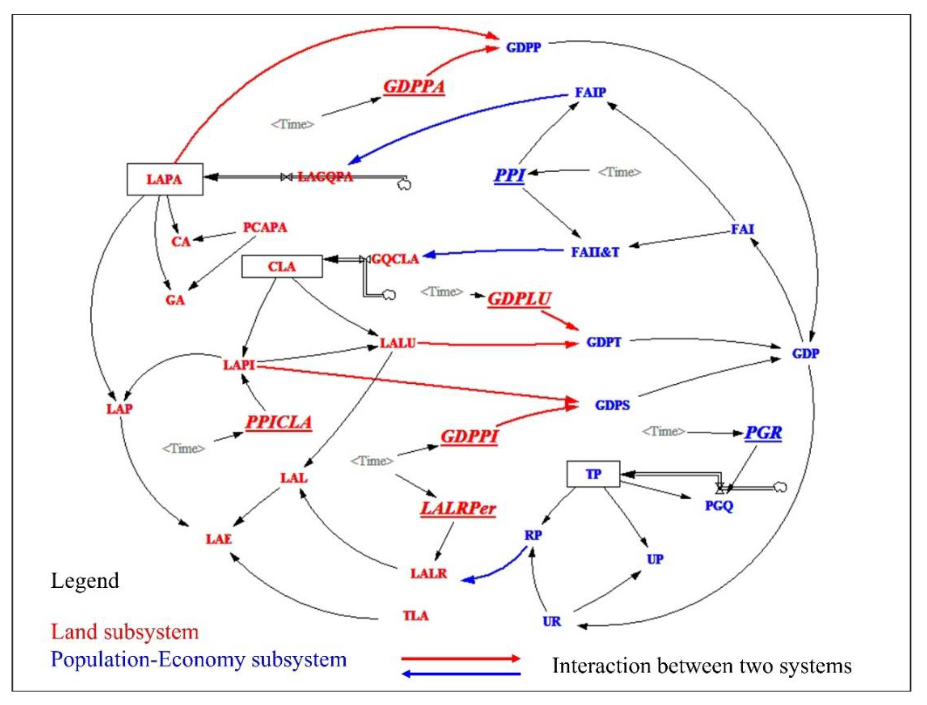
The structure optimization model of PLE space is realized by constructing the system dynamic model. First, it is necessary to clarify the system boundary and system structure. The system boundary affects the model’s complexity, and the boundary cannot be too large or too small. The system structure refers to the variables involved in the model and the relationship between them. The purpose of this research is to understand the interaction between the main elements in PLE space. Therefore, the system boundary was confined to Zhaotong from 2010 to 2017, and the model was constructed by selecting factors related to population, social fixed asset investment, regional GDP, land resources, and more. The PLE space system is divided into a population–economy subsystem and a land-use subsystem. According to data recorded by the Statistical Yearbook of Zhaotong and Statistical Bulletin of Zhaotong, 33 variables were finally selected. The system structure is shown in Figure 4. Specific variable names and units are detailed in Table S1 of the supplementary file.
The relationship between system variables and mathematical equations is the core of the model construction, and it influences the accuracy of the model. In this paper, the comprehensive empirical method, regression analysis method, logical inference method, weighted average method, and other methods are used to determine the equation parameters. Moreover, the Lookup function and conditional function provided by Vensim software were fully utilized, and 33 groups of equations were finally determined (see Equations (S1)–(S33) in the methods and data of the supplementary file for details).
The simulated values were compared with the actual values of some variables from 2010 to 2017, and the results are shown in Table S2. The absolute values of the errors are in the range of 0–5%, which indicates that the constructed model can respond to the interrelationships among the elements within a reasonable range and can be used for future simulation.
2.3. FLUS Model
2.3.1. Parameters
The FLUS model is employed to realize the spatial layout of PLE land use. The detailed theory and process can be found in Liu’s article [41]. Parameters mainly used in the model are described as follows:
- (1)
- Suitability probability
The suitability probability of different land types on each parcel can be calculated based on the powerful, intelligent prediction function of the FLUS model’s neural network by inputting the historical data of driving factors related to land-use evolution. The amount of future land demand is determined by other methods. In this study, SD is coupled with FLUS to simulate the spatial layout of the PLE space of Zhaotong city in 2030.
The selection of driving factors is crucial to the ANN-based suitability probability. This paper references previous literature studies [52,53,54]. Sixteen driving factors of different aspects of land use were taken into account, such as topography (including elevation, slope, and slope direction), natural meteorology (including soil conditions, precipitation, and annual mean air temperature), and social economy (including population, GDP, distance from the city center, commuting time). Data sources are shown in Table 3. All raster datasets were resampled to 30 m by the software Arcgis 10.2.
- (2)
- Conversion cost matrix
The cost matrix reflects the conversion rules between different land types, in which 0 means that one type of land is not allowed to be converted to another, 1 means that it can be converted. The conversion cost matrix for different land types in this paper varies during model validation and scenario simulation.
- (3)
- Neighborhood factor values
Referring to the method of Ou et al. [55] and expert empirical knowledge, the neighborhood weights of the nine land types in this paper were determined, as shown in Table 4. The weight values range from 0 to 1. A value closer to 1 represents a stronger expansion capacity.
- (4)
- Other parameters
Another parameter is the time t in the formula, representing the number of iterations. More iterations mean more time and lower efficiency. To fully carry out spatial simulation and take simulation efficiency into account at the same time, the number of iterations is set as 600 and the acceleration factor as 0.5.
2.3.2. Verification
The feasibility and effectiveness of the FLUS model should be verified at first. In this paper, land use data from 2010 and 2015 are used as the base period data to simulate those of 2015 and 2018, respectively.
Firstly, the suitability probabilities of different land types in 2010 and 2015 were calculated using artificial neural networks (ANNs). Accuracy can be measured by the indicators RMSE (root mean square error), ROC (receiver operating characteristic), and AUC (area under curve) [41]. Smaller RMSE values and larger AUC values indicate higher model accuracy. Results showed that the RMSE was 0.2464 in 2010 and 0.2471 in 2015. AUC values corresponding to the ROC curves are shown in Table 5. ROC curves are shown in Figures S1 and S2.
Secondly, conversion cost matrices used for verification are obtained from the transition matrix between the years 2010~2015 and 2015~2018. If there is a conversion happened between two land classes during the above period, it is assigned as 1; otherwise, it is assigned as 0. They are shown in Tables S3 and S4, respectively. Other parameters are the same as those described in the Parameters section.
Results showed that compared with the actual data, the kappa coefficient (an indicator used to measure accuracy) of the 2015 simulation is 0.91, with an overall accuracy of 93.35%. The confusion matrix (a specific table layout that allows visualization of the performance of an algorithm in the field of machine learning) between the actual data and simulation is shown in Tables S5 and S6. Similarly, the kappa coefficient of the 2018 simulation is 0.85, with an overall accuracy of 88.99%. Both kappa coefficients are greater than or equal to 0.85, indicating that the FLUS model has high simulation accuracy and can be used for future simulations.
2.4. Constrained Scenarios
Base scenarios and optimization scenarios are designed to fully simulate the future PLE space layout of Zhaotong city in 2030. The optimization scenarios include Scenario A, in which production and living development are given priority; Scenario B, in which ecological protection is given priority; and Scenario C, in which both are considered. In addition, three levels (high level, medium level, and low level) are designed in every optimization scenario. The details are shown in Table 6.
There are two main aspects in which the above scenarios differ. On the one hand, the control variables’ values are different in the system dynamics model for quantitative optimization. On the other hand, the transformation rules are different when using the FLUS model for spatial simulation.
Five different approaches are chosen as optimization projects in the PLE space system dynamics model, including land-use efficiency promotion, industrial structure adjustment, agricultural production space protection, intensive development of construction land, and controlling population growth. Relevant control variables in the model are listed in Table 7. The variables associated with the land-use efficiency promotion are mainly related to the GDP output per land (including GDPPA, GDPPI, and GDPLU). In the base scenario, i.e., at the previous rate of development, the values are 0.05, 11.58, and 9.10, respectively, by 2030. Based on the expert experience, on this basis, the optimization is carried out assuming that at high, medium, and low levels; GDPPA increases by 100%, 60%, and 30%, respectively; GDPPI increases by 60%, 30%, and 10%, respectively, and GDPLU increases by 120%, 80%, and 50% respectively. The values obtained are presented in Table 7. The values of the other variables for the different scenarios are also listed in Table 7.
The cost matrix of the base scenario is simple; that is, the urban living land use cannot be converted into another land use, and the conversion between other different land types is unrestricted. See Table S7 for the detailed cost matrix. No masking of the restricted area is performed.
The development scenario of giving production-living development priority (Scenario A) ensures that the improvement of production space and living space is fully considered. The expansion of production-living space comes at the expense of occupying ecological space. In the stage of spatial simulation, urban living space cannot be converted into others and is the same as priority agricultural production space and general agricultural production space (see Tables S8 and S9 for the detailed cost matrix). At the high and medium levels, the restricted ecological space vector scope of 2018 is used as a mask area; that is, the land parcels within the mask scope are no longer involved in the subsequent land-use conversion process. However, there is no mask at low levels.
The ecological space is fully protected in the context of Scenario B. For spatial simulation, urban living space cannot be converted into other land use and is the same as priority ecological space and general ecological space (see Tables S10 and S11 for the detailed cost matrix). Other settings are like Scenario A.
A balanced development scenario (Scenario C) means that the priority ecological space and priority agricultural production space are fully protected. During the spatial simulation, urban living space cannot be converted into another land use, and the same requirements are made for the priority ecological space and priority agricultural production space (see Tables S12 and S13 for the detailed cost matrix). Other settings are similar to Scenario A.
Only the industrial production space area, urban living space area, and rural living space area can be directly obtained from the simulation results of the system dynamic model. Other PLE space needs to be calculated according to the proportion of subclasses to the upper-class land in 2018, especially in the base scenario and Scenario B, in which ecological space protection is given priority. In Scenario A, the areas of priority agricultural production space and general agricultural production space were the same as those in 2018, and others were obtained by the above method. In Scenario C, the priority ecological space and priority agricultural production space were not less than those in 2018, and others were obtained by the above method.
3. Results
3.1. Spatiotemporal Pattern of PLE Space: Economic Development Is Related to the Decline of Ecological Space and General Agricultural Production Space
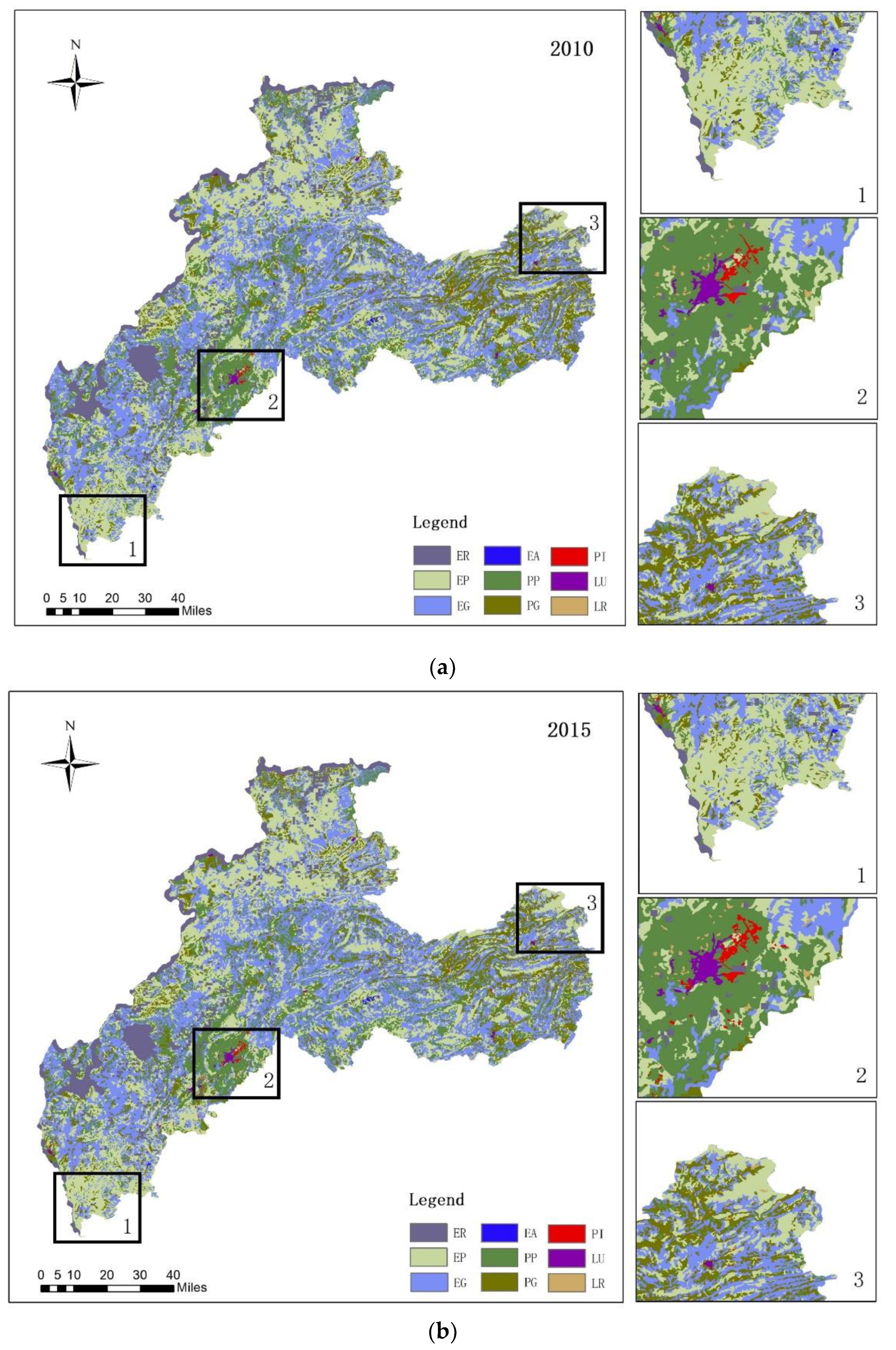
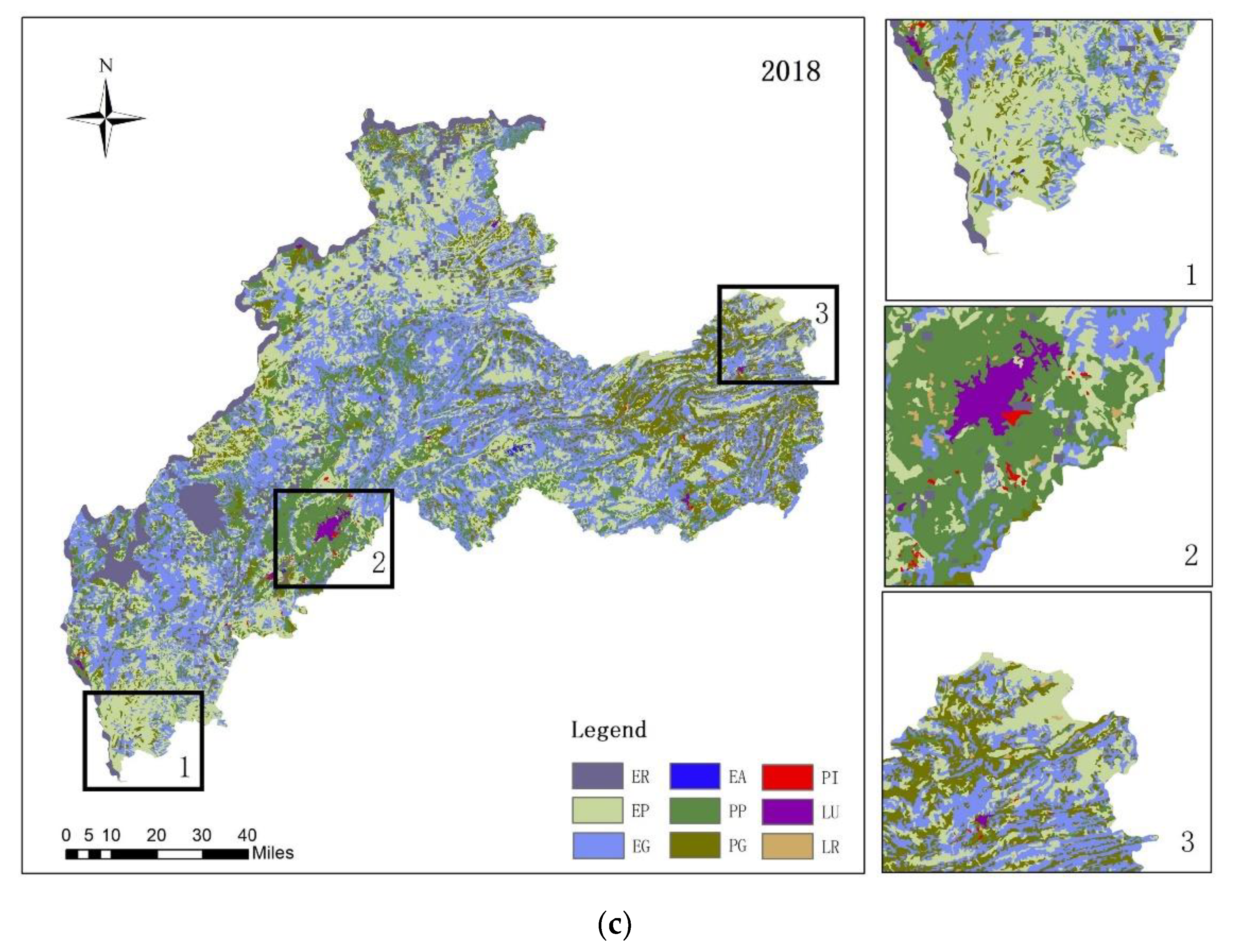
The spatial distribution of PLE spaces is shown in Figure 5. Restricted ecological space (ER) is mainly distributed in the western part of Zhaotong city, but it is more concentrated in the southwestern part. The priority ecological space (EP) is distributed in the south and northwest of the city. The general ecological space (EG) is more scattered. The area of accommodated ecological space (EA) is small. Priority agricultural production space (PP) is distributed in the city’s central part and is more concentrated and contiguous, while general agricultural production space (PG) is in the northeastern part. In addition, industrial production space (PI), urban living space (LU), and rural living space (LR) are more scattered.
The land areas of the PLE spaces in 2010, 2015, and 2018 are shown in Table S14. Detailed subclass areas are shown in Table S15. Table S20 shows that the ecological space extends over an area of more than 16,200 km2, accounting for more than 72% of the total, followed by the production space at approximately 6000 km2, accounting for approximately 27%, and then by the living space, the smallest area at only approximately 1%. Among ecological spaces, the areas of priority ecological space and general ecological space accounted for more than 90%. Living spaces are mainly rural living space, accounting for approximately 70%.
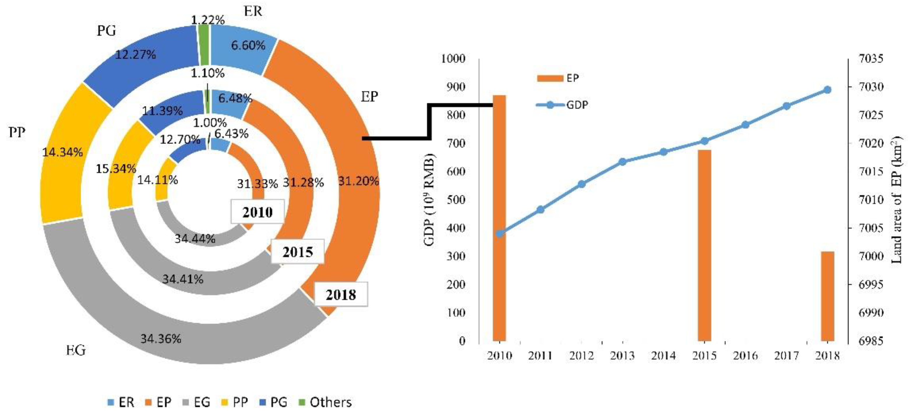
In terms of changing trends, the ecological space area decreased from 2010 to 2018 but not significantly. Figure 6 shows that between 2010 and 2018, Zhaotong’s GDP continued to increase, while at the same time, the space for priority ecological space continued to decrease. Conversely, production space decreased significantly from 6031 km2 in 2010 to 6000 km2 in 2018, which was mainly due to the decrease in general agricultural production space. There was a clear trend of growth in living space, from 194.67 km2 in 2010 to 232.97 km2 in 2018, with an increase of approximately 20%. This increase is mainly due to the expansion of urban living space, which was only 40.78 km2 in 2010, reaching 72.76 km2 in 2018, with an increase of approximately 78%.
The transfer matrix between 2010 and 2015 is shown in Table S16. The most significant growth between 2010 and 2015 was in industrial production space, which increased from 15.74 to 32.75 km2. The expansion of industrial production space mainly encroached on priority agricultural production space (8.69 km2) and priority ecological space (4.96 km2), accounting for 51% and 29% of the expansion space, respectively. The main distribution of industrial space is in the central region. The most significant growth between 2015 and 2018 was in urban living space, which increased from 42.97 to 72.76 km2 (Table S17). Urban living space expansion mainly encroached on priority agricultural production space (16.74 km2) and industrial production space (12 km2), accounting for 56% and 41% of the total expansion space, respectively. This change in use was concentrated in the central region.
3.2. Assessment of the Optimization Scenarios from the View of Total Amount: A High Level of Development Is More Conducive for Achieving the Planned Target of 2030
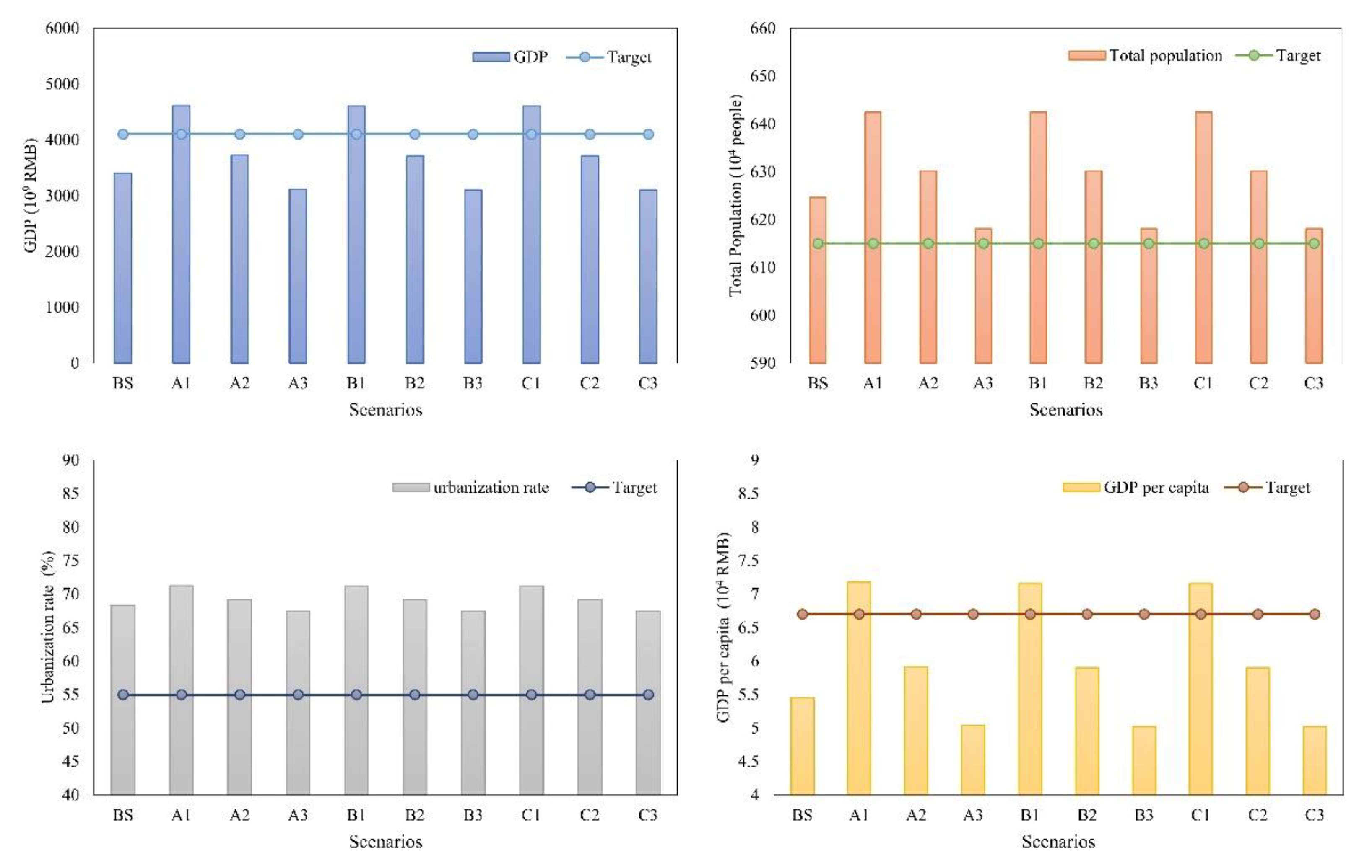
The planning goal for economic and social development in the “Urban Master Planning of Zhaotong City (2011–2030)” was used as a basis for reference. The economic development target is to reach a regional GDP of 410 billion RMB and a per capita GDP of approximately 67,000 RMB by 2030. For the social development target, the total population is 6.15 million, and the urbanization rate is 55%.
Based on the constructed SD model of PLE space, the simulated values of the main variables under different scenarios in 2030 were obtained, as shown in Table S18. This result indicates that under the base scenario, the regional GDP is 340.508 billion yuan by 2030, with a total population of 6,245,700 people, the GDP per capita of 54,500 yuan, and an urbanization rate of 68.33%. This means that under the base scenario, the regional GDP and GDP per capita cannot meet the planning target, although the population and urbanization rate can.
As shown in Table S18 and Figure 7, A1, B1, and C1 can meet the planning requirements. The remaining six scenarios show the opposite. Under Scenario A1, the regional GDP is 461.444 billion yuan by 2030, the total population is approximately 6.424 million, the GDP per capita is 71.8 thousand yuan, and the urbanization rate is 71.27%. Since the difference between Scenario B and Scenario C is mainly reflected in the constraints on agricultural space during spatial allocation, the quality is the same. Under Scenarios B and C, the regional GDP is 460.220 billion yuan, the total population is 6,424,400 people, the GDP per capita is 71,600 yuan, and the urbanization rate is 71.24%.
3.3. Assessment of the Optimization Scenarios from the View of Spatial Configuration: High Levels of Development Will Lead to Further Expansion of Industrial Production Space and Living Space
The land area of PLE space in 2030 under different scenarios and the changes in terms of percentage compared with 2018 are listed in Table 8. Under the base scenario, urban living space (LU) is approximately 1.2 times larger than that in 2018, while rural living space (LR) decreases by approximately one-third (33.32%). The production land-use area shrinks from 6000.09 to 5760.48 km2, a decrease of approximately 4%, and priority agricultural production space and general agricultural production space shrink by 5.91%, while industrial production space grows by 3.8 times. This implies that the expansion of urban living space and industrial production space is very evident in the base scenario, while priority agricultural production space and industrial production space are the most occupied.
Under Scenario A1, because of the protection of agricultural production space, the expansion of living space and industrial production space leads to different degrees of reduction in ecological space. Ecological space decreases by 1.49%, industrial production space and urban living space increase by 241.56% and 194.98%, and rural living space increases by 3.7%. Under Scenario B1, there is a slight decrease in ecological space (approximately 0.01%). The expansion of living space and industrial production space is at the expense of agricultural production space, resulting in a 3.66% decrease. Compared with Scenario B1, the priority agricultural production space is protected with constraints in Scenario C1, leading to the general agricultural production space being further reduced by 7.93%.
3.4. Optimization Pattern of the Coordinated Development: Production–Living Space Should Be Given Priority
The spatial optimization efficiency is evaluated by whether the spatial allocation can reach the future total amount required. When the FLUS model is used for the spatial layout, the number of requirements may not be reached for the same 600 iterations due to the different constraint rules. The percentage difference between the actual number of configurations and the demands is used as the spatial optimization efficiency indicator.
The future demand area of different land types needs to be proportionally converted to the number of land parcels in the FLUS model for spatial simulation. The gap between the actual allocation of parcels and the demand parcels is also presented in Table S19. In the base scenario, the expansion of rural living space far exceeds the planned demand by approximately 38%. In contrast, the number of allocated parcels of industrial production space differs from the number of demands by −22.63%, which means that it does not meet the target. In Scenario A1, 25.37% of the urban living space does not meet the future demand in the spatial configuration. In Scenario B1, neither urban living space nor industrial production space meets future needs; for example, the gap in urban living space is −22.14%. This is more obvious in Scenario C1, where 55.23% of the urban living space does not meet the demand.
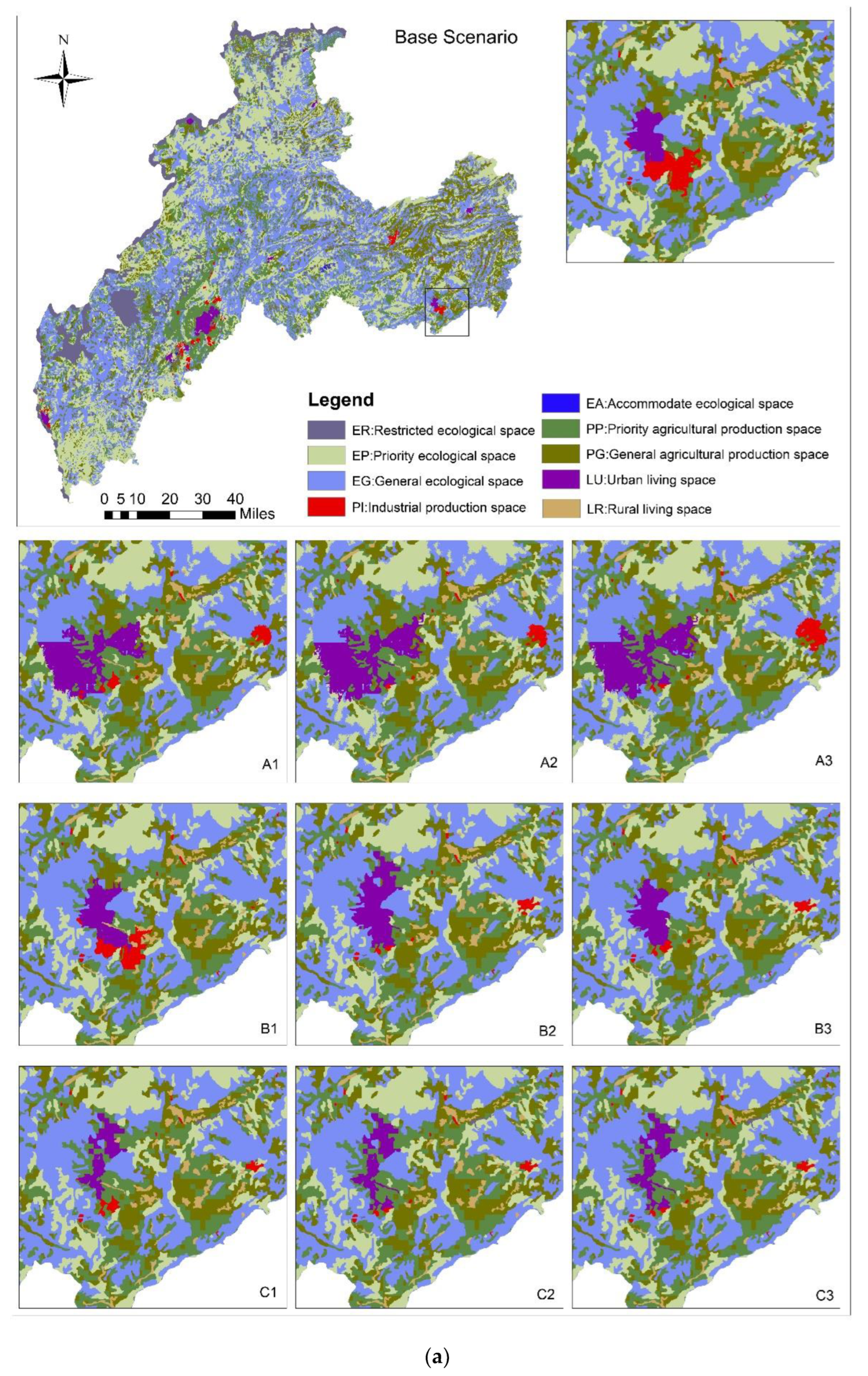
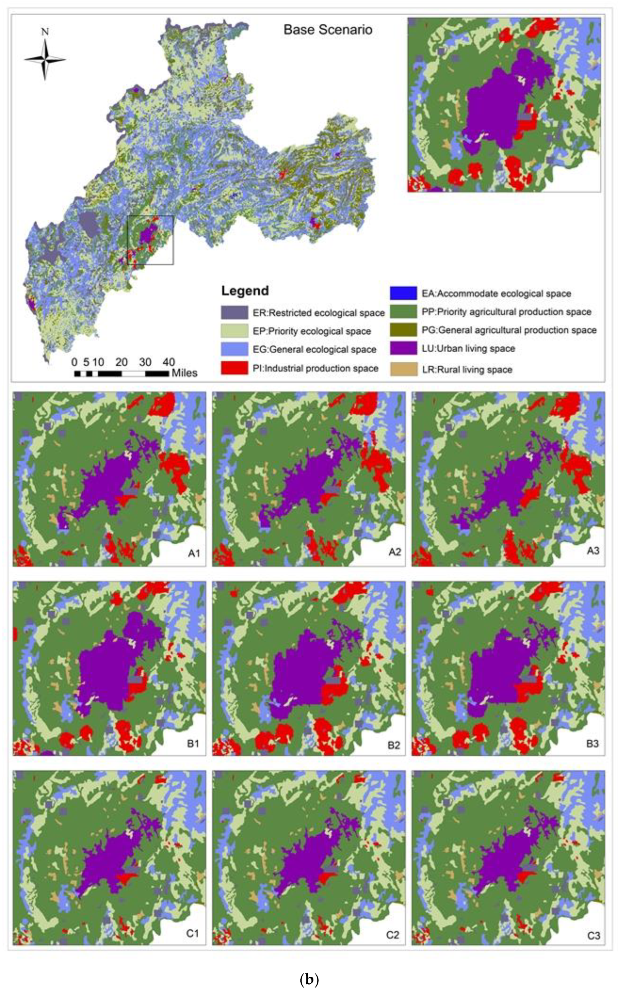
Since the differences in several scenarios are mainly reflected in urban living space and industrial production space, the central and eastern regions are compared in separate enlargements (see Figure 8). Compared with 2018, the expansion of urban living space in the base scenario is mainly in the central region, centering on the original urban living space and expanding further outward. The expansion of industrial production space is also distributed in the central part but in a scattered manner around the central city, with the exception of two concentrated locations in the eastern region (see Figure 8).
Unlike the base scenario, the urban living space expands to the southwest with a small-scale agglomeration in Scenario A, and the same phenomenon occurs in the eastern part. In contrast, the expansion of industrial production space tends to extend to the south compared to the base scenario. The expansion of urban living space is very similar at different levels under Scenario B. Only Scenario B1 shows a clustering distribution in the northern part of the original urban living space and a relatively smaller degree of clustering in the eastern part. However, the industrial production space is not obvious in other scenarios except for a more obvious expansion at B1, especially in the northeastern region. In Scenario C, the expansion of urban living space and industrial production space is somewhat limited and only slightly expands compared to 2018, again mainly in the central and eastern regions.
4. Conclusions and Implications
4.1. Findings
Results show that the model has high accuracy and can be combined with local policy to simulate the PLE space under future scenarios:
- (1)
- Combined with the actual situation of Zhaotong city, the accuracy of the SD model is more than 95%. Absolute values of the errors are in the range of 0–5%, which indicates that the constructed model can respond to the interrelationships among the social and natural elements within a reasonable range and can be used for future simulation.
- (2)
- The suitability probabilities of different land types were calculated using artificial neural networks (ANNs). Accuracy in terms of RMSE is both about 0.24. Additionally, AUC values corresponding to the ROC curves are all between 0.6~1. To a certain extent, it means that selective factors related to land use suitability are effective and the ANN method performs well.
- (3)
- In the stage of spatial simulation by FLUS, confusion matrices describe the wrong allocation between simulated and actual spatial distribution. The related kappa coefficients are both above 0.85.
As a typical area with a backward economy and limited geographical conditions, Zhaotong city has unique characteristics of PLE space. Talking about the future development direction and whether the planning objectives can be achieved, the model constructed in this paper gives these answers:
- (1)
- The ratio of ecological space, production space, and living space is approximately 7.2:2.7:0.1. Almost all the production space is agricultural production space, accounting for approximately 99%. Living space is dominated by rural living space, accounting for approximately 70%. Between 2010 and 2018, Zhaotong’s GDP continued to increase, while at the same time, the space for priority ecological space continued to decrease. Zhaotong city has seen a significant expansion of living space and industry space in recent decades, which has greatly encroached on agricultural production space, especially in the central region, which is the core of the city.
- (2)
- The planning requirements for 2030 can only be met under Scenarios A1, B1, and C1. This means that Zhaotong needs further improvements in land-use efficiency, industrial structure adjustments, and intensive development. However, considering suitability and space allocation rules, the demand for urban living space and industrial production space and the spatial allocation of land types could not be fully realized in the simulation time (600 iterations). Except for A3, where the configuration of all nine land types could meet the requirements, the demand for urban living space or industrial production space in other scenarios is far from satisfied.
- (3)
- Production and living space should be given priority in future development. A higher level of development is still needed in terms of policies and measures. When planning future PLE space, the layout of urban living space and industrial production space should be given priority, especially in the central and south-central regions as well as the eastern region.
4.2. Contributions
The study of the PLE space is important for the planning of regional sustainable development. Complicatedly, it involves geographical, ecological, and economic knowledge and experiments, requiring integrated research. This paper built an integrated optimization model by which PLE space can be simulated quantitatively and spatially, which enriches the current study of PLE. Additionally, it can be a powerful tool.
The SD model constructed takes local demographic and economic factors into account from a system science perspective. The mathematical relationships between the main factors are quantified by establishing equation and simulation parameters as a way to simulate the mechanism of urban operation. The FLUS model, based on the suitability probability using an ANN, is carried out in a roulette wheel way by considering the cost matrix, neighborhood influence, and other factors. For example, some constraints, as well as planning objectives, are embedded into the model in a parametric way, and the land allocation operations in the actual planning process are restored by different land class conversion rules.
In contrast to the multi-objective optimization model, which is often used to find the optimal solution [32], the coupled model in this paper can simulate the urban operation mechanism at a more microscopic scale and perform dynamic derivation in both time and space dimensions simultaneously with more flexible parameter adjustment. Moreover, this paper sets a variety of development scenarios in the form of parameters for the relevant indicators in local policies and assists in decision-making based on the simulation results. For Zhaotong city, economic development and environmental protection are advocated to be given equal importance. For other cities that also face urban development planning problems, the case study of this paper can provide inspiration.
4.3. Limitations and Future Research
Like all research, there are some limitations to this study. For example, there is no clearly defined relationship between the urbanization rate and GDP, and the urbanization rate is influenced by many factors [38,56]. To simplify the SD model, the equation parameters between the two can only be determined using regression analysis and referring to the development trend of other cities. In addition, adequate surveys involving stakeholders and local policy can also improve the rationality of the scenario simulation. However, this requires more comprehensive and in-depth preliminary research, which is also an aspect that can be considered for further studies.
In addition, only taking Zhaotong, a city located in southwest China, as a case study is far from enough. For planning problems in other cities with different geographical and natural endowments, the applicability of the model needs more work to be carried out to verify the model. Additionally, urban sustainability is a common issue around the world, but the solutions to different problems need to be contextualized in a variety of ways. Regardless of the approach taken, the rights of stakeholders should be considered when making decisions [57,58].
Supplementary Materials
The following supporting information can be downloaded at: https://0-www-mdpi-com.brum.beds.ac.uk/article/10.3390/land11030411/s1, Table S1: Names, units and data sources of the variables included in the PLE space system dynamics model; Table S2: Comparison of simulated and real values of some key variables; Table S3: Cost Matrix for the 2015 simulation using 2010 PLE spatial distribution data; Table S4: Cost Matrix for the 2015 simulation using 2010 PLE spatial distribution data; Table S5: Confusion matrix between the actual and simulated values of PLE in 2015; Table S6: Confusion matrix between the actual and simulated values of PLE in 2018; Table S7: Cost Matrix for Base Scenario; Table S8: Cost Matrix for Scenario A1 and A2; Table S9: Cost Matrix for Scenario A3; Table S10: Cost Matrix for Scenario B1 and B2; Table S11: Cost Matrix for Scenario B3; Table S12: Cost Matrix for Scenario C1 and C2; Table S13: Cost Matrix for Scenario C3; Table S14: Ratio of land area for production, living and ecological space in 2010, 2015, and 2018; Table S15: Land area and percentage of 9 subclasses in PLE space in 2010, 2015, and 2018; Table S16: Land-use transition matrix from 2010 to 2015; Table S17: Land-use transition matrix from 2015 to 2018; Table S18: Projections of the economy and population under different scenarios in 2030; Table S19: Difference between future demand and allocated values for different scenarios; Figure S1: ROC curves and AUC values for 2010 suitability probability results based on ANN; Figure S2: ROC curves and AUC values for 2015 suitability probability results based on ANN.
Author Contributions
D.W.: conceptualization; methodology; validation; formal analysis; investigation; writing—original draft preparation; writing—review and editing; visualization. J.F.: conceptualization; writing—review and editing; supervision; project administration. D.J.: supervision; project administration; funding acquisition. All authors have read and agreed to the published version of the manuscript.
Funding
This research was funded by the Strategic Priority Research Program of the Chinese Academy of Sciences (XDA19040305), Youth Innovation Promotion Association (Grant No. 2018068).
Institutional Review Board Statement
Not applicable.
Informed Consent Statement
Not applicable.
Data Availability Statement
Not applicable.
Conflicts of Interest
The authors declare no conflict of interest.
References
- Galvani, A.P.; Bauch, C.T.; Anand, M.; Singer, B.H.; Levin, S.A. Human-environment interactions in population and ecosystem health. Proc. Natl. Acad. Sci. USA 2016, 113, 14502–14506. [Google Scholar] [CrossRef] [Green Version]
- Lin, C.L. Evaluating the urban sustainable development strategies and common suited paths considering various stakeholders. Environ. Dev. Sustain. 2022, 1–42. [Google Scholar] [CrossRef]
- What are Coupled Human-Environment System? GEOG: 30N: Environment and Society in a Changing World. Available online: https://www.e-education.psu.edu/geog30/node/325 (accessed on 15 February 2022).
- Scholz, R.W.; Binder, C.R. Princles of Human-Environment Systems (HES) Research. In Proceedings of the 2nd International Congress on Environmental Modelling and Software, Osnabrück, Germany, 1–7 June 2004; Volume 116. Available online: https://scholarsarchive.byu.edu/iemssconference/2004/all/116 (accessed on 26 February 2022).
- Turner, B.L.; Matson, P.A.; McCarthy, J.J.; Corell, R.W.; Christensen, L.; Eckley, N.; Hovelsrud-Broda, G.K.; Kasperson, J.X.; Kasperson, R.E.; Luers, A.; et al. Illustrating the coupled human-environment system for vulnerability analysis: Three case studies. Proc. Natl. Acad. Sci. USA 2003, 100, 8080–8085. [Google Scholar] [CrossRef] [Green Version]
- Katramiz, T.; Okitasari, M. Accelerating 2030 Agenda Integration: Aligning National Development Plans with the Sustainable Development Goals; United Nations University Institute for the Advanced Study of Sustainability (UNU-IAS): Tokyo, Japan, 2021; Volume 25. [Google Scholar]
- Australian Government, Department of Agriculture, Water and the Environment. 2030 Agenda for Sustainable Development and the Sustainable Development Goals. Available online: https://www.awe.gov.au/environment/international/2030-agenda (accessed on 15 February 2022).
- Government of Canada. Towards Canada’s 2030 Agenda National Strategy. Available online: https://www.canada.ca/en/employment-social-development/programs/agenda-2030/national-strategy.html#h2.06 (accessed on 15 February 2022).
- The Department of Strategic Policy, Planning and Aid Coordination, Republic of Vanuatu. Vanuatu 2030 the People Plan: National Sustainable Development Plan 2016 to 2030; The Department of Strategic Policy, Planning and Aid Coordination, Republic of Vanuatu: Port Vila, Vanuatu, 2016; Available online: https://www.nab.vu/sites/default/files/documents/Vanuatu%20Sustainable%20Dev.%20Plan%202030-EN_0.PDF (accessed on 15 February 2022).
- Barbier, E.B.; Burgess, J.C. Sustainable development goal indicators: Analyzing trade-offs and complementarities. World Dev. 2019, 122, 295–305. [Google Scholar] [CrossRef]
- United Nations. The Sustainable Development Goals Report 2018; United Nations: New York, NY, USA, 2018. [Google Scholar]
- Nilsson, M.; Griggs, D.; Visbeck, M. Map the interactions between Sustainable Development Goals. Nature 2016, 534, 320–322. [Google Scholar] [CrossRef]
- Von Stechow, C.; Minx, J.C.; Riahi, K.; Jewell, J.; McCollum, D.L.; Callaghan, M.W.; Bertram, C.; Luderer, G.; Baiocchi, G. 2 degrees C and SDGs: United they stand, divided they fall? Environ. Res. Lett. 2016, 11, 15. [Google Scholar] [CrossRef]
- Wang, Y.P.; Zhou, X.N. The year 2020, a milestone in breaking the vicious cycle of poverty and illness in China. Infect. Dis. Poverty 2020, 9, 8. [Google Scholar] [CrossRef] [Green Version]
- Yang, Y.Y.; de Sherbinin, A.; Liu, Y.S. China’s poverty alleviation resettlement: Progress, problems and solutions. Habitat Int. 2020, 98, 13. [Google Scholar] [CrossRef]
- Bao, C.; He, D.M. Scenario Modeling of Urbanization Development and Water Scarcity Based on System Dynamics: A Case Study of Beijing-Tianjin-Hebei Urban Agglomeration, China. Int. J. Environ. Res. Public Health 2019, 16, 19. [Google Scholar] [CrossRef] [Green Version]
- Chen, J. Rapid urbanization in China: A real challenge to soil protection and food security. Catena 2007, 69, 1–15. [Google Scholar] [CrossRef]
- Bai, X.M.; Chen, J.; Shi, P.J. Landscape Urbanization and Economic Growth in China: Positive Feedbacks and Sustainability Dilemmas. Environ. Sci. Technol. 2012, 46, 132–139. [Google Scholar] [CrossRef] [PubMed]
- Wang, Q. Effects of urbanisation on energy consumption in China. Energy Policy 2014, 65, 332–339. [Google Scholar] [CrossRef]
- Huang, J.C.; Lin, H.X.; Qi, X.X. A literature review on optimization of spatial development pattern based on ecological-production-living space. Prog. Geogr. 2017, 36, 378–391. [Google Scholar]
- Sachs, J.D. From Millennium Development Goals to Sustainable Development Goals. Lancet 2012, 379, 2206–2211. [Google Scholar] [CrossRef]
- Bansal, P. Evolving sustainably: A longitudinal study of corporate sustainable development. Strateg. Manag. J. 2005, 26, 197–218. [Google Scholar] [CrossRef]
- Saci, H.; Berezowska-Azzag, E. Food security and urban sustainability of alternative food models: Multicriteria analysis based on Sustainable Development Goals and Sustainable Urban Planning. Cah. Agric. 2021, 30, 35. [Google Scholar] [CrossRef]
- Grah, B.; Dimovski, V.; Peterlin, J. Managing Sustainable Urban Tourism Development: The Case of Ljubljana. Sustainability 2020, 12, 792. [Google Scholar] [CrossRef] [Green Version]
- Khosravi, S.; Lashgarara, F.; Poursaeed, A.; Najafabadi, M.O. Modeling the relationship between urban agriculture and sustainable development: A case study in Tehran city. Arab. J. Geosci. 2022, 15, 97. [Google Scholar] [CrossRef]
- Balletto, G.; Ladu, M.; Milesi, A.; Camerin, F.; Borruso, G. Walkable City and Military Enclaves: Analysis and Decision-Making Approach to Support the Proximity Connection in Urban Regeneration. Sustainability 2022, 14, 457. [Google Scholar] [CrossRef]
- Wu, Z.Y.; Shan, J.J. Study on the Evolution and Optimization Countermeasures of “Ecological-production-living Space” Pattern. City 2019, 10, 15–26. [Google Scholar]
- Zhang, C.H. Study on Conflict Measure and Optimization of Coastal Zone Based on the Ecological-Production-Living Spaces—A Case Study of Zhuang He in Dalian. Ph.D. Thesis, Liaoning Normal University, Dalian, China, June 2018. [Google Scholar]
- Wang, J. Study on spatial reconstruction and optimization of “sansheng” in mining area—Take dexing copper mine in jiangxi province as an example. Master’s Thesis, East China University of Technology, Nanchang, China, June 2016. [Google Scholar]
- Zhou, L.Q. The Study on the Optimization and Function Improvement of “Ecological-Production-Living” Space in Zhengzhou. Master’s Thesis, Zhengzhou University, Zhengzhou, China, May 2018. [Google Scholar]
- Anderson, C.B.; Seixas, C.S.; Barbosa, O.; Fennessy, M.S.; Diaz-Jose, J.; Herrera-F., B. Determining nature’s contributions to achieve the sustainable development goals. Sustain. Sci. 2019, 14, 543–547. [Google Scholar] [CrossRef]
- Ye, Y.C. Spatial Layout Optimization of Industrial-Living-Ecological Land in Yingtan City Based on Spatial Decision-Making. Ph.D. Thesis, Jiangxi Agricultural University, Nanchang, China, June 2018. [Google Scholar]
- Gunantara, N.J.C.E. A review of multi-objective optimization: Methods and its applications. Cogent Eng. 2018, 5, 1502242. [Google Scholar] [CrossRef]
- Wang, H.D.; Olhofer, M.; Jin, Y.C. A mini-review on preference modeling and articulation in multi-objective optimization: Current status and challenges. Complex Intell. Syst. 2017, 3, 233–245. [Google Scholar] [CrossRef]
- Yeh, S.C.; Wang, C.A.; Yu, H.C. Simulation of soil erosion and nutrient impact using an integrated system dynamics model in a watershed in Taiwan. Environ. Modell. Softw. 2006, 21, 937–948. [Google Scholar] [CrossRef]
- Wei, S.K.; Yang, H.; Song, J.X.; Abbaspour, K.C.; Xu, Z.X. System dynamics simulation model for assessing socio-economic impacts of different levels of environmental flow allocation in the Weihe River Basin, China. Eur. J. Oper. Res. 2012, 221, 248–262. [Google Scholar] [CrossRef]
- Wingo, P.; Brookes, A.; Bolte, J. Modular and spatially explicit: A novel approach to system dynamics. Environ. Modell. Softw. 2017, 94, 48–62. [Google Scholar] [CrossRef]
- Gu, C.L.; Ye, X.Y.; Cao, Q.W.; Guan, W.H.; Peng, C.; Wu, Y.T.; Zhai, W. System dynamics modelling of urbanization under energy constraints in China. Sci. Rep. 2020, 10, 16. [Google Scholar] [CrossRef]
- Abadi, L.S.K.; Shamsai, A.; Goharnejad, H. An analysis of the sustainability of basin water resources using Vensim model. KSCE J. Civ. Eng. 2015, 19, 1941–1949. [Google Scholar] [CrossRef]
- Lloyd, H.; Amos, M. Analysis of Independent Roulette Selection in parallel ant colony optimization. In Proceedings of the Genetic and Evolutionary Computation Conference; Association for Computing Machinery: New York, NY, USA, 2017; pp. 19–26. [Google Scholar]
- Liu, X.P.; Liang, X.; Li, X.; Xu, X.C.; Ou, J.P.; Chen, Y.M.; Li, S.Y.; Wang, S.J.; Pei, F.S. A future land use simulation model (FLUS) for simulating multiple land use scenarios by coupling human and natural effects. Landsc. Urban Plan. 2017, 168, 94–116. [Google Scholar] [CrossRef]
- Liang, X.; Liu, X.P.; Li, X.; Chen, Y.M.; Tian, H.; Yao, Y. Delineating multi-scenario urban growth boundaries with a CA-based FLUS model and morphological method. Landsc. Urban Plan. 2018, 177, 47–63. [Google Scholar] [CrossRef]
- Liang, X.; Liu, X.P.; Li, D.; Zhao, H.; Chen, G.Z. Urban growth simulation by incorporating planning policies into a CA-based future land-use simulation model. Int. J. Geogr. Inf. Sci. 2018, 32, 2294–2316. [Google Scholar] [CrossRef]
- Lin, W.B.; Sun, Y.M.; Nijhuis, S.; Wang, Z.L. Scenario-based flood risk assessment for urbanizing deltas using future land-use simulation (FLUS): Guangzhou Metropolitan Area as a case study. Sci. Total Environ. 2020, 739, 10. [Google Scholar] [CrossRef] [PubMed]
- Mooney, H.A.; Duraiappah, A.; Larigauderie, A. Evolution of natural and social science interactions in global change research programs. Proc. Natl. Acad. Sci. USA 2013, 110, 3665–3672. [Google Scholar] [CrossRef] [PubMed] [Green Version]
- Mortada, S.; Abou Najm, M.; Yassine, A.; El Fadel, M.; Alamiddine, I. Towards sustainable water-food nexus: An optimization approach. J. Clean. Prod. 2018, 178, 408–418. [Google Scholar] [CrossRef]
- Veldhuis, A.J.; Yang, A.D. Integrated approaches to the optimisation of regional and local food-energy-water systems. Curr. Opin. Chem. Eng. 2017, 18, 38–44. [Google Scholar] [CrossRef]
- Nie, Y.L.; Avraamidou, S.; Xiao, X.; Pistikopoulos, E.N.; Li, J.; Zeng, Y.J.; Song, F.; Yu, J.; Zhu, M. A Food-Energy-Water Nexus approach for land use optimization. Sci. Total Environ. 2019, 659, 7–19. [Google Scholar] [CrossRef] [PubMed] [Green Version]
- Zhaotong Bureau of Statistics. Zhaotong Statistical Yearbook 2018; Zhaotong Bureau of Statistics: Zhaotong, China, 2018. [Google Scholar]
- Forest Resources Overview of Yunnan Province in 2018. Available online: http://lcj.yn.gov.cn/html/2019/zuixindongtai_1219/55160.html (accessed on 2 April 2020).
- Xie, H.L.; Zhang, Y.W.; Zeng, X.J.; He, Y.F. Sustainable land use and management research: A scientometric review. Landsc. Ecol. 2020, 35, 2381–2411. [Google Scholar] [CrossRef]
- Li, M.; Wu, J.J.; Deng, X.Z. Identifying Drivers of Land Use Change in China: A Spatial Multinomial Logit Model Analysis. Land Econ. 2013, 89, 632–654. [Google Scholar] [CrossRef]
- Ni, J.P.; Shao, J.A. The Drivers of Land Use Change in the Migration Area, Three Gorges Project, China: Advances and Prospects. J. Earth Sci. 2013, 24, 136–144. [Google Scholar] [CrossRef]
- Xu, X.M.; Jain, A.K.; Calvin, K.V. Quantifying the biophysical and socioeconomic drivers of changes in forest and agricultural land in South and Southeast Asia. Glob. Chang. Biol. 2019, 25, 2137–2151. [Google Scholar] [CrossRef]
- Ouyang, X.; He, Q.; Zhu, X. Simulation of Impacts of Urban Agglomeration Land Use Change on Ecosystem Services Value under Multi-Scenarios: Case Study in Changsha-Zhuzhou-Xiangtan Urban Agglomeration. Econ. Geogr. 2020, 40, 93–102. [Google Scholar]
- Chen, M.X.; Zhang, H.; Liu, W.D.; Zhang, W.Z. The Global Pattern of Urbanization and Economic Growth: Evidence from the Last Three Decades. PLoS ONE 2014, 9, 15. [Google Scholar] [CrossRef] [PubMed] [Green Version]
- Stein, S. Capital City: Gentrification and the Real Estate State; Verso Books: Brooklyn, NY, USA, 2019. [Google Scholar]
- Sklair, L. The Icon Project: Architecture, Cities, and Capitalist Globalization; Oxford University Press: New York, NY, USA, 2017. [Google Scholar]
Figure 1.
The relationship of PLE space and SDGs.

Figure 2.
Location and slope map of Zhaotong city.

Figure 3.
Workflow for the optimization.

Figure 4.
Interrelationship diagram of the PLE system dynamics model. Variables in underlined italics are control variables.
Figure 4.
Interrelationship diagram of the PLE system dynamics model. Variables in underlined italics are control variables.

Figure 5.
(a–c) represent the spatial distribution of PLE space in 2010, 2015, and 2018, respectively.ER is restricted ecological space. EP is priority ecological space. EG is general ecological space. EA is accommodated ecological space. PP is priority agricultural production space. PG is general agricultural production space. PI is industrial production space. LU is urban living space. LR is rural living space.


Figure 6.
Changing trends of PLE space and GDP from 2010 to 2018.

Figure 7.
Development target in 2030 and simulation results of different scenarios.

Figure 8.
Spatial distribution of PLE space in different scenarios: (a) represent eastern region; (b) represent central region. And A1–C3 represent differen scenarios.
Figure 8.
Spatial distribution of PLE space in different scenarios: (a) represent eastern region; (b) represent central region. And A1–C3 represent differen scenarios.


Table 1.
Data sources for the “PLE Spaces” classification.
| Datasets | Type | Spatial Resolution | Year | Data Source |
|---|---|---|---|---|
| Multi-period land cover dataset of China | Raster | 30 m | 2010 2015 2018 | Resource and Environment Science and Data Center http://www.resdc.cn/ (accessed on 15 May 2020) |
| Nature reserve boundary data of China | Shapefile | —— | 2018 | Resource and Environment Science and Data Center http://www.resdc.cn/ (accessed on 15 May 2020) |
| Dataset of primary rivers spatial distribution in China | Shapefile | —— | 2000 | |
| Ecological Function Reserves of China | Shapefile | —— | 2010 | |
| Importance of Ecological Service Functions of China | Raster | 1 km | 2010 | Ecosystem Assessment and Ecological Security Database http://www.ecosystem.csdb.cn/ (accessed on 15 May 2020) |
| Ecosystem Sensitivity of China | Raster | 1 km | 2010 | |
| GDP (Gross domestic product) | Raster | 1 km | 2010 2015 2018 | Resource and Environment Science and Data Center http://www.resdc.cn/ (accessed on 15 May2020) |
| NPP (Net primary productivity) | Raster | 500 m | 2010 2015 2018 | LAADS DAAC https://ladsweb.nascom.nasa.gov/search (accessed on 15 May 2020) |
Table 2.
Relationship between the classification system of PLE spaces and MLC classification.
| Class | Subclass | MLC Classification and Codes |
|---|---|---|
| Ecological Space | Restricted ecological space (ER) | National nature reserves area, extremely important ecological services areas, first-class rivers area, ecologically extremely sensitive areas, and waters area (4) |
| Priority ecological space (EP) | High-coverage grass (31), Mid-coverage grass (32), Wooded land (21) | |
| General ecological space (EG) | Shrubland (22), Sparse woodland (23), Low-coverage grass (33) | |
| Accommodated ecological space (EA) | Marshland (64), Bare rocky gravel land (66) | |
| Production Space | Priority agricultural production space (PP) | Both arable land (1) and other woodland (24) with above-average GDP or NPP |
| General agricultural production space (PG) | Both arable land (1) and other woodland (24) with below-average GDP or NPP | |
| Industrial production space (PI) | Other construction land (53) | |
| Living Space | Urban living space (LU) | Urban building land (51) |
| Rural living space (LR) | Rural settlements (52) |
Table 3.
Driving factors and data sources.
| Categories | Data | Spatial Resolution | Data Source |
|---|---|---|---|
| Terrain and Landforms | Elevation, slope, and direction | 90 m | Resource and Environment Science and Data Center http://www.resdc.cn/ (accessed on 2 April 2020) |
| Soil conditions | Nutrient availability Nutrient retention capacity Rooting conditions Oxygen availability to roots Excess salts Toxicity Workability (constraining field management) | 10 km | Harmonized World Soil Database v 1.2 http://www.fao.org/soils-portal/data-hub/soil-maps-and-databases/harmonized-world-soil-database-v12/en/ (accessed on 2 April 2020) |
| Precipitation and Temperature | Annual average precipitation Annual average temperature | 1 km | Resource and Environment Science and Data Center http://www.resdc.cn/ (accessed on 2 April 2020) |
| Socio-economic | Population | 1 km | The Gridded Population of the World, Version 4 (GPWv4) https://0-doi-org.brum.beds.ac.uk/10.7927/H4F47 M65( accessed on 2 April 2020) |
| GDP per capita | 1 km | Dryad: Gridded global datasets for Gross Domestic Product and Human Development Index over 1990–2015 https://0-doi-org.brum.beds.ac.uk/10.5061/dryad.dk1j0 (accessed on 2 April 2020) | |
| Distance to city center | 100 m | Euclidean distance calculated using city coordinate data | |
| Travel Time | 1 km | European Commission Joint Research Centre Global Environment Monitoring Unit http://forobs.jrc.ec.europa.eu/products/gam/(2008) (accessed on 2 April 2020) |
Table 4.
Neighborhood factor values for different PLE subclasses.
| ER | EP | EG | EA | PP | PG | PI | LU | LR |
|---|---|---|---|---|---|---|---|---|
| 0.01 | 0.01 | 0.01 | 0.01 | 0.19 | 0.67 | 0.81 | 1.00 | 1.00 |
Table 5.
AUC values based on ANN suitability probability calculation results.
| AUC | ER | EP | EG | EA | PP | PG | PI | LU | LR |
|---|---|---|---|---|---|---|---|---|---|
| 2010 | 0.85 | 0.63 | 0.61 | 0.88 | 066 | 0.73 | 0.90 | 0.97 | 0.78 |
| 2015 | 0.84 | 0.63 | 0.62 | 0.91 | 0.68 | 0.72 | 0.84 | 0.98 | 0.77 |
Table 6.
Scenario design and solution code.
| Scenarios Name | Abbreviations | ||
|---|---|---|---|
| Base Scenario | BS | ||
| Optimization Scenarios | High level | Medium level | Low level |
| Giving priority to production-living development scenario (A) | A1 | A2 | A3 |
| Giving priority to ecological protection scenario (B) | B1 | B2 | B3 |
| Both are considered in scenario (C) | C1 | C2 | C3 |
Table 7.
Base scenario and parameter settings at different levels.
| Approaches | Variables 1 | Base Scenario | High Level | Medium Level | Low Level |
|---|---|---|---|---|---|
| Land-use efficiency promotion | GDPPA | 0.05 | 0.05 | 0.04 | 0.03 |
| GDPPI | 11.58 | 18.04 | 14.66 | 12.40 | |
| GDPLU | 9.10 | 11.58 | 9.47 | 7.89 | |
| Industrial structure adjustment | PPICLA | 47 | 32 | 36 | 41 |
| Agricultural production space protection | PPI | 2.35 | 0.85 | 1.00 | 1.50 |
| Controlling population growth | PGR | 0.85 | 1.15 | 1.00 | 0.85 |
| Intensive development of construction land | LALRPer | 0.54 | 0.90 | 0.75 | 0.60 |
1 Definition of variables can be found in Table S1.
Table 8.
Land area of the PLE spaces in 2030 and changes compared with 2018 under different scenarios.
Table 8.
Land area of the PLE spaces in 2030 and changes compared with 2018 under different scenarios.
| ER | EP | EG | EA | PP | PG | PI | LU | LR | |
|---|---|---|---|---|---|---|---|---|---|
| 2018 | 1481.17 | 7000.82 | 7710.14 | 11.74 | 3218.38 | 2752.14 | 29.57 | 72.76 | 160.21 |
| BS | 1499.88 | 7089.26 | 7807.54 | 11.89 | 3028.17 | 2589.49 | 142.82 | 161.06 | 106.83 |
| Change% | 1.26 | 1.26 | 1.26 | 1.28 | −5.91 | −5.91 | 382.99 | 121.36 | −33.32 |
| A1 | 1481.17 | 6896.57 | 7595.33 | 11.57 | 3218.38 | 2752.14 | 101.00 | 214.63 | 166.14 |
| Change% | 0.00 | −1.49 | −1.49 | −1.49 | 0.00 | 0.00 | 241.56 | 194.98 | 3.70 |
| A2 | 1481.17 | 6910.55 | 7610.73 | 11.59 | 3218.38 | 2752.14 | 110.44 | 196.33 | 145.60 |
| Change% | 0.00 | −1.29 | −1.29 | −1.29 | 0.00 | 0.00 | 273.49 | 169.84 | −9.12 |
| A3 | 1466.79 | 6932.87 | 7635.31 | 11.63 | 3218.38 | 2752.14 | 122.65 | 176.49 | 120.67 |
| Change% | −0.97 | −0.97 | −0.97 | −0.97 | 0.00 | 0.00 | 314.77 | 142.57 | −24.68 |
| B1 | 1481.17 | 7000.36 | 7709.63 | 11.74 | 3100.69 | 2651.50 | 100.98 | 214.58 | 166.29 |
| Change% | 0.00 | −0.01 | −0.01 | −0.01 | −3.66 | −3.66 | 241.49 | 194.91 | 3.80 |
| B2 | 1481.17 | 7012.31 | 7722.80 | 11.76 | 3103.00 | 2653.48 | 110.41 | 196.29 | 145.72 |
| Change% | 0.00 | 0.16 | 0.16 | 0.16 | −3.58 | −3.58 | 273.39 | 169.77 | −9.05 |
| B3 | 1489.38 | 7039.63 | 7752.89 | 11.81 | 3085.17 | 2638.23 | 122.61 | 176.44 | 120.77 |
| Change% | 0.55 | 0.55 | 0.55 | 0.55 | −4.14 | −4.14 | 314.65 | 142.50 | −24.62 |
| C1 | 1481.17 | 7000.82 | 7709.17 | 11.74 | 3218.38 | 2533.80 | 100.98 | 214.58 | 166.29 |
| Change% | 0.00 | 0.00 | −0.01 | −0.01 | 0.00 | −7.93 | 241.49 | 194.91 | 3.80 |
| C2 | 1481.17 | 7012.31 | 7722.80 | 11.76 | 3218.38 | 2538.10 | 110.41 | 196.29 | 145.72 |
| Change% | 0.00 | 0.16 | 0.16 | 0.16 | 0.00 | −7.78 | 273.39 | 169.77 | −9.05 |
| C3 | 1489.38 | 7039.63 | 7752.89 | 11.81 | 3218.38 | 2505.02 | 122.61 | 176.44 | 120.77 |
| Change% | 0.55 | 0.55 | 0.55 | 0.55 | 0.00 | −8.98 | 314.65 | 142.50 | −24.62 |
Publisher’s Note: MDPI stays neutral with regard to jurisdictional claims in published maps and institutional affiliations. |
© 2022 by the authors. Licensee MDPI, Basel, Switzerland. This article is an open access article distributed under the terms and conditions of the Creative Commons Attribution (CC BY) license (https://creativecommons.org/licenses/by/4.0/).
Share and Cite
MDPI and ACS Style
Wang, D.; Fu, J.; Jiang, D. Optimization of Production–Living–Ecological Space in National Key Poverty-Stricken City of Southwest China. Land 2022, 11, 411. https://0-doi-org.brum.beds.ac.uk/10.3390/land11030411
AMA Style
Wang D, Fu J, Jiang D. Optimization of Production–Living–Ecological Space in National Key Poverty-Stricken City of Southwest China. Land. 2022; 11(3):411. https://0-doi-org.brum.beds.ac.uk/10.3390/land11030411
Chicago/Turabian StyleWang, Di, Jingying Fu, and Dong Jiang. 2022. "Optimization of Production–Living–Ecological Space in National Key Poverty-Stricken City of Southwest China" Land 11, no. 3: 411. https://0-doi-org.brum.beds.ac.uk/10.3390/land11030411
Note that from the first issue of 2016, this journal uses article numbers instead of page numbers. See further details here.