An Investigation of Particle Swarm Optimization Topologies in Structural Damage Detection

Abstract

In the past few decades, vibration-based structural damage detection (SDD) has attracted widespread attention. Using the response data of engineering structures, the researchers have developed many methods for damage localization and quantification. Adopting meta-heuristic algorithms, in which particle swarm optimization (PSO) is the most widely used, is a popular approach. Various PSO variants have also been proposed for improving its performance in SDD, and they are generally based on the Global topology. However, in addition to the Global topology, other topologies are also developed in the related literature to enhance the performance of the PSO algorithm. The effects of PSO topologies depend significantly on the studied problems. Therefore, in this article, we conduct a performance investigation of eight PSO topologies in SDD. The success rate and mean iterations that are obtained from the numerical simulations are considered as the evaluation indexes. Furthermore, the average rank and Bonferroni-Dunn’s test are further utilized to perform the statistic analysis. From these analysis results, the Four Clusters are shown to be the more favorable PSO topologies in SDD.

1. Introduction

In the last two decades, vibration-based structural damage detection (SDD) has received considerable attention since the dynamic responses of engineering structures are easy to obtain. The main idea is that the structural dynamic responses can be regarded as a function of its physical parameters (mass, stiffness, and damping). Hence, the presence of damage leads to the change of modal parameters, such as natural frequencies, mode shapes, and structural flexibility. The objective of SDD is to infer the physical parameters from the measured response data to locate and quantify structural damage. Therefore, vibration-based SDD belongs to a typical inverse problem [1,2].

Nowadays, various popular meta-heuristic algorithms have been developed to solve this inverse problem in SDD. When compared with the traditional optimization algorithms [3], such as Newton’s method and the gradient descent method, they are effective and robust in coping with uncertainties and incomplete information. The meta-heuristic algorithms [4] mainly simulate the physical laws or biological phenomena in nature, and they use simple coding methods to represent various practical problems. In different meta-heuristic algorithms, the PSO algorithm has received extensive attention because of its few parameters, fast convergence, and easy implementation. The PSO algorithm is a population-based meta-heuristic that was proposed by Kennedy and Eberhart [5]. It is based on simulating the foraging behavior of bird flocking, and it has been widely used in many fields, such as benchmark function optimization [6], image processing [7], scheduling decision [8], and engineering [9]. However, it is well-known that the classical PSO algorithm yields premature convergence. Consequently, various PSO variants have been proposed to alleviate this phenomenon in different research fields. When dealing with the SDD problem, the improvement of the algorithm mainly includes hybrid PSO schemes [10,11,12] and multi-stage PSO schemes [13,14,15].

In all of these recent works in SDD, only the Global topology is considered, which is the most commonly used one. In the Global topology, all of the particles are connected. Each particle adjusts its position according to its self-experience and global social experience. In addition to the Global topology, other topologies [16,17,18] have also been developed to enhance the performance of the PSO algorithm. A proper PSO topology can alleviate premature convergence and improve search efficiency [19]. Therefore, it is crucial to study the effects of PSO topologies on the performance of the studied problems. Cheng [19] examined the influences of four topologies, namely Global, Local, Four Clusters, and Von Neumann, on the population diversity in benchmark functions. The experimental results demonstrated that the Ring topology performs better than others. Andrich [20] analyzed the performances of Global, Local, and Von Neumann topologies in Neural Networks training, but all of these three topologies exhibit overfitting and non-convergent behaviors. Figueiredo et al. studied the effects of five topologies (Global, Local, Von Neumann, Wheel, and Four Clusters) on PSO performance in extreme learning machines [21]. The results showed that the Global topology is more promising than other topologies. From the literature, it can be concluded that there is no one best topology for all issues, and the performances of PSO topologies depend significantly on the studied problems. However, to the best of our knowledge, there is no research on the effects of different PSO topologies in SDD. Therefore, this paper investigates the performances of eight PSO topologies in the SDD of a cantilever beam.

This paper is organized, as follows: in Section 2, the basic principles of SDD are briefly introduced. Section 3 presents the definition of the basic PSO and the characteristics of eight topologies. In Section 4, the performances of different topologies are compared under single-damage and multi-damage scenarios of a cantilever beam. Finally, Section 5 concludes this work and gives the topology guideline for SDD. Some future works are depicted.

2. Structural Damage Detection

2.1. Problem Formulation

For an undamped system, the structure can be discretized into D elements while using the finite element methods (FEM), and the structural characteristic equation is expressed as:

$$(\mathbf{K}-{\lambda }_s\mathbf{M}){\mathsf{\Phi }}_s=0,(s=1,2,\dots ,m)$$

(1)

where $\mathbf{M}$ is the global mass matrix, $\mathbf{K}$ is the global stiffness matrix, ${\lambda }_s$ indicates the sth eigenvalue of the structure, and ${\mathsf{\Phi }}_s$ denotes the sth mode shape. Subsequently, $\mathbf{M}$ and $\mathbf{K}$ are assembled by the corresponding element matrices:

$$\mathbf{K}=\sum _{j=1}^D{\mathbf{k}}_j$$

(2a)

$$\mathbf{M}=\sum _{j=1}^D{\mathbf{m}}_j$$

(2b)

where ${\mathbf{k}}_j$ is the jth element stiffness matrix, ${\mathbf{m}}_j$ is the jth element mass matrix, and D is the number of elements of the structure.

In this paper, an Euler–Bernoulli beam is modeled using the FEM. The beam is discretized into a number of D elements, with the displacement and slope as nodal degrees of freedom and cubic interpolation function. For a uniform beam of length L, the mass matrix and the stiffness matrix of each beam element are given, as follows:

$${\mathbf{m}}^{\mathbf{e}}=\frac{\rho Al}{420}\left[\begin{array}{cccc}156& 22l& 54& -13l\\ 22l& 4l^2& 13l& -3l^2\\ 54& 13l& 156& -22l\\ -13l& -3l^2& -22l& 4l^2\end{array}\right]$$

(3)

$${\mathbf{k}}^{\mathbf{e}}=\frac{EI}{l^3}\left[\begin{array}{cccc}12& 6l& -12& 6l\\ 6l& 4l^2& -6l& 2l^2\\ -12& -6l& 12& -6l\\ 6l& 2l^2& -6l& 4l^2\end{array}\right]$$

(4)

where $l=L/D$ is the finite element length, $\rho$ is the mass density, A is the cross-section area, E is Young’s modulus, and I is the moment of inertia. Subsequently, convert the local coordinate system to the global coordinate system, the global mass matrix $\mathbf{M}$, and global stiffness matrix $\mathbf{K}$ can be obtained using Equations (2a) and (2b).

A scenario should first be defined in order to simulate any damage in the structure. In fact, each damage scenario is a D-dimensional vector, and the jth component of the vector represents the damage to the structure. In this study, the damage is modeled using the Young’s modulus reduction, and the decrease in mass is negligible [22]. Assuming that the element stiffness of the structure is uniformly reduced after damage, then the reduction factor is used to indicate damage:

$${\alpha }_j=\frac{E-E_j}{E}$$

(5)

where E and $E_j$ are the Young’s modulus of the jth element before and after the damage. ${\alpha }_j\in [0,1]$ and ${\alpha }_j=0$ mean no damage, while ${\alpha }_j=1$ indicates a complete loss of the element stiffness, and $\alpha =({\alpha }_1,{\alpha }_2,\dots ,{\alpha }_D)$ is the damage vector of the structure.

This definition is profitable, because it allows for estimating not only the severity of the damage, but also its location at the elemental level. When considering the damage vector $\alpha$, the stiffness matrix $\mathbf{K}$ after the damage is changed as:

$${\mathbf{K}}^d=\sum _{j=1}^D(1-{\alpha }_j){\mathbf{k}}_j$$

(6)

where ${\mathbf{K}}^d$ is the global stiffness matrix after damage.

2.2. Fitness Function

The FEM-based SDD is an optimization problem. Defining a fitness function that can minimize the discrepancy of the response between the measurement and model is one of the essential steps in optimization.

Because the natural frequencies of the structure are easy to obtain with high accuracy, a fitness function that is composed of pure natural frequencies is considered. An efficient correlation-based index (ECBI) was introduced in [23] to formulate the fitness function, which is expressed as follows:

$$\begin{array}{c}\hfill S\left(\alpha \right)=-\frac{1}{2}\left[\frac{{\left|\mathsf{\Delta }{F}^T·\delta F\left(\alpha \right)\right|}^2}{\left(\mathsf{\Delta }{F}^T·\mathsf{\Delta }F\right)\left(\delta F^T\left(\alpha \right) · \delta F\left(\alpha \right)\right)}+\frac{1}{m}\sum _{s=1}^m\frac{min\left(f_s^d,f_s\left(\alpha \right)\right)}{max\left(f_s^d,f_s\left(\alpha \right)\right)}\right]\end{array}$$

(7)

where $\mathsf{\Delta }F$ is the change of natural frequency vector before and after damage, which is defined as:

$$\mathsf{\Delta }F=\left\{\mathsf{\Delta }{f}_s=\frac{f_s^h-f_s^d}{f_s^h}\right\}(s=1,2,\dots ,m)$$

(8)

where $f_s^h$ and $f_s^d$ are the sth component of the healthy (undamaged) natural frequency vector $F_h$ and damaged natural frequency vector $F_d$, respectively.

$\delta F\left(\alpha \right)$ represents the change of natural frequency vector that is predicted by FEM with regard to the healthy natural frequency vector, which is denoted as:

$$\delta F\left(\alpha \right)=\left\{\delta f_s\left(\alpha \right)=\frac{f_s^h-f_s\left(\alpha \right)}{f_s^h}\right\}(s=1,2,\dots ,m)$$

(9)

where $\alpha =({\alpha }_1,{\alpha }_2,\dots ,{\alpha }_D)$ is the damage vector and $f_s\left(\alpha \right)$ is the sth component of the natural frequency vector that is predicted by the FEM. In this article, $m=9$ is used uniformly. Besides, when compared with other forms of the fitness function composed of pure natural frequencies, the superiority of fitness function that is shown in Equation (7) has been demonstrated in [24].

The objective of SDD is to search for a specific damage vector ${\alpha }^{*}$ for which its predicted natural frequency vector exactly matches with the modeled damage vector $\alpha$. When ${\alpha }^{*}=\alpha$, this fitness function reaches its minimum value of −1. Therefore, the SDD problem is transformed into an inverse optimization problem:

$$\begin{array}{cc}\hfill & argminS\left({\alpha }^{*}\right)\hfill \\ \hfill & \mathrm{where}{\alpha }^{*}=({\alpha }_1^{*},{\alpha }_2^{*},\dots ,{\alpha }_D^{*})\hfill \\ \hfill & \mathrm{subject}\mathrm{to}{\alpha }_j^{*}\in [0,1](1\le j\le D)\hfill \end{array}$$

(10)

Subsequently, the optimization algorithms, such as the popular PSO algorithm, can be employed to find a damage vector ${\alpha }^{*}$ to minimize Equation (7).

3. Particle Swarm Optimization

3.1. Basic Model

The PSO algorithm is inspired by the foraging behavior of birds and it is widely used to solve optimization problems. Each bird in the flock is called a particle, the PSO algorithm contains a population composed of a certain number of particles, and each particle represents a potential solution. All of the particles fly in a D-dimensional search space, each particle has its own position and velocity, and the fitness function is used to judge its quality. The whole population is randomly initialized, and then each particle evolves toward the best ones through iteration. Suppose that there is a swarm consisting of N particles in a D-dimensional search space, and the current position of the particle i can be expressed as a vector $X_i={(x_{i1},x_{i2},\dots ,x_{iD})}^T$, $i=1,2,\dots ,N$; the velocity of the particle i is $V_i={(v_{i1},v_{i2},\dots ,v_{iD})}^T$. In the tth iteration, the particle updates its velocity and position by tracking the personal best position ($pbest$) and global best position ($gbest$), as follows [25]:

$$\begin{array}{c}\hfill v_{ij}(t+1)=\omega v_{ij}\left(t\right)+c_1{r}_{1ij}(pbes{t}_{ij}\left(t\right)-x_{ij}\left(t\right))+c_2{r}_{2ij}(gbes{t}_j\left(t\right)-x_{ij}\left(t\right))\end{array}$$

(11)

$$x_{ij}(t+1)=x_{ij}\left(t\right)+v_{ij}(t+1)$$

(12)

where t is the number of iterations, $j=1,2,\dots ,D$; $v_{ij}\left(t\right)$ and $x_{ij}\left(t\right)$ are the jth components of the position and the velocity of particle i at iteration t, and $pbes{t}_{ij}\left(t\right)$ and $gbes{t}_j\left(t\right)$ represent the jth components of the personal best location and the global best location, respectively. $\omega$ is the inertia weight, and it reflects the impact of the particle’s current velocity on the next iteration. $r_{1ij}$, $r_{2ij}$ are random numbers that are uniformly distributed between $[0,1]$; $c_1$ and $c_2$ are the acceleration coefficients, $c_1$ controls the tendency of the particle towards its personal best location, and $c_1$ adjusts the trend of the particle approaching the global best location. The particle updates itself by tracking the $pbest$ and $gbest$ until the termination criteria are satisfied. During the search process, in order to avoid the invalid search, the position and velocity are limited to a certain interval $\left[X_{min}{X}_{max}\right]$ and $[-V_{max}{V}_{max}]$, which are generally set by the user.

The main steps of the PSO algorithm are given, as follows:

(1)

Initialize the position and velocity of the particles.

(2)

Calculate the fitness value $S\left(X_i\right)$$(i=1,2,\cdots ,N)$ using Equation (7).

(3)

For each particle $X_i$, compare its fitness value $S\left(X_i\right)$ with the local best location $S\left(pbes{t}_i\right)$ that it has experienced. If $S\left(X_i\right)<S\left(pbes{t}_i\right)$, update it as the current personal best position.

(4)

For each particle $X_i$, compare its personal best fitness value $S\left(pbes{t}_i\right)$ with the global best fitness value $S\left(gbest\right)$. If $S\left(pbes{t}_i\right)<S\left(gbest\right)$, update it as the current global best position.

(5)

Adjust the velocity and position of the population according to Equations (11) and (12), also perform the boundary condition.

(6)

If the algorithm reaches the maximum number of iterations or the minimum value of the fitness function, stop the algorithm, and output the result; if not, go to step (2).

3.2. PSO Topologies

The PSO topologies describe the neighbor relationship and interaction between particles, which can control the propagation of information in the particle swarm and directly affect the particle swarm’s optimization ability and convergence. The PSO topologies can be divided into two categories: static topologies and dynamics topologies. For static topologies, each particle’s neighborhood does not change in the whole optimization process; for dynamics topologies, the neighborhoods of some individuals vary during the iterations. Subsequently, some commonly used static topologies and dynamic topologies are briefly introduced.

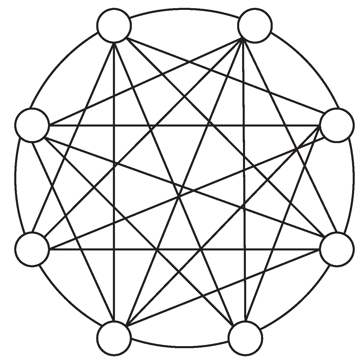
1. Global topology: the Global topology is the most widely used in the literature. Each particle is directly connected to all other particles in the swarm and is each other’s neighbors, so the particles can quickly exchange information, as illustrated in Figure 1. Thus, the algorithm with this topology can achieve convergence fast, but there is a risk of falling into a local optimum [16].

2. Local topology: in the Local topology, the particles are directly connected to their m immediate neighbors. When $m=2$, each particle only has two neighbors, as illustrated in Figure 2. Different regions in the search space can be simultaneously explored by using this topology [17].

3. Von Neumann topology: the Von-Neumann topology is a grid structure, as shown in Figure 3; each particle is connected to its four neighbors: top, bottom, left, and right.

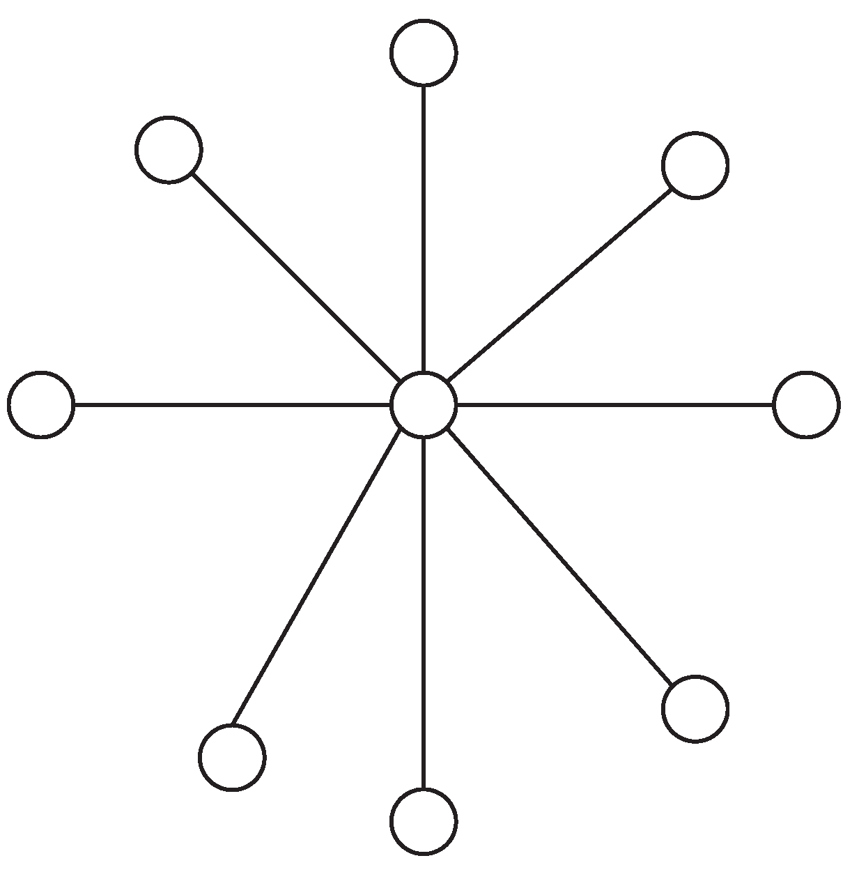
4. Wheel topology: as shown in Figure 4, the particles using the Wheel topology are isolated from each other, and one particle is randomly selected as the focal point for all information flow.

5. Four Clusters topology: there are four subgroups in the four clusters topology, as displayed in Figure 5. The particles in each subgroup spread information under Global topology; each subgroup communicates with each other through three particles.

6. Clan topology: the Clan topology is a type of dynamic topology that was proposed by Carvalho et al. [17], in which the swarm is divided into several subgroups, called clans. The particles in each clan adjust their positions under the fully-connected structure (Global topology). Figure 6 shows an example of four clans (A, B, C, and D) used in this article. Each clan has five particles and the particle with the best fitness is selected as the leader of the clan in each iteration. In Figure 6, the leaders of ${\mathrm{A}}_3$, ${\mathrm{B}}_5$, ${\mathrm{C}}_5$, and ${\mathrm{D}}_1$ are marked in gray. Subsequently, a conference between the leaders occurs. In the conference, only the leaders of each clan are employed to perform a new PSO search. The leaders’ members may change during the search process. When the conference takes place, it can use the Global or Local topologies to exchange information and is referred to as Clan Global topology and Clan Local topology. As shown in Figure 7, the Clan Global topology adopts the global information propagation mechanism among the leaders, enhancing the exploitation ability. In the Clan Local topology of Figure 8, the leaders take the local information propagation mechanism that can strengthen their exploration ability.

7. Multi-Ring topology: the dynamic topology proposed in [18] is based on coupling different ring layers. There are n layers of this topology, and each layer has the same number of particles, as shown in Figure 9. The particles in the Multi-Ring topology take the same communication way as with the Von Neumann topology, except that the particles in the first layer do not communicate with the final layer. Thus, consider a layer k, one particle $k_i$ will exchange information with its neighbors being denoted as $(k_{i-1},k_{i+1},{k-1}_i,{k+1}_i)$ when $1<k<n$. Otherwise, when $k=1$ or $k=n$, the neighbors of the particle $k_i$ are $(k_{i-1},k_{i+1},{k+1}_i)$, and $(k_{i-1},k_{i+1},{k-1}_i)$, respectively. Moreover, the ‘rotation skill’ is added in this topology in order to reduce the possibility of falling into a local optimum. Thus, if the layer does not improve its own best location in $t_r$ iterations, it will be rotated. A rotation example can be seen in Figure 10. It can be seen that the three layers of particles are named from a to i, and the particle e communicates with its neighbors {d, f, b, h}. After the rotation, its neighborhood is changed to {d, f, a, g}. More generally, the index of each particle in this layer is changed to $i=(i+d)mod\left(nl\right)$, where d is the rotation distance and $nl$ is the particle numbers in the layer. In this article, $t_r=20,nl=4,d=2$, according to the recommendations presented in [18].

4. Numerical Simulations for SDD of the Cantilever Beam

Figure 11 is a 2D finite element model of the cantilever beam structure. The length of the beam is 1 m, and thirty identical finite elements are considered.

Table 1. The physical parameters of the beam structure.

Young Modulus E (Pa)	Poisson Ratio ν	Density ρ (Kg·m−3)	Width w (m)	Thickness d (m)
$2.0\times {10}^{11}$ N/m${}^2$	0.33	7850	$2.49\times {10}^{-2}$ m	$5.3\times {10}^{-3}$ m

provides the physical parameters of the beam structure.

Single damage and multiple damages are all considered to evaluate the performance of different PSO topologies. Nine damage cases with different sites and degrees are assumed in the paper, as displayed in

Table 2. Damage scenarios for the cantilever beam.

Damage Scenarios	Types	Elements	Severity
1	I	8 (Front)	20%
2		15 (Middle)	30%
3		25 (End)	50%
4	II	5, 6 (Neighbor)	10%, 10%
5		13, 18 (Symmetrical)	20%, 50%
6		15, 25	20%, 30%
7	III	5, 6, 25	30%, 30%, 20%
8		10, 16, 22	30%, 30%, 30%
9		15, 19, 20	10%, 10%, 10%

. According to the number of damaged elements, those scenarios are classified into three categories: type I is composed of cases with one damage element; type II has cases with two damage elements; and, type III is the scenarios with three damage elements.

The parameter settings of the PSO algorithm are outlined, as follows:

• Initialization: the positions of the initial population are randomly created in the search space, and the initial velocities of the population are set to zero to prevent the swarm explosion at the beginning of the algorithm [26].
• Boundary conditions: according to the guidance in [27,28], the following restricted boundary condition is used, and $Vmax=Xmax$:

  $$\begin{array}{cccc}\hfill if{x}_{ij}& >X_{max}\hfill & \hfill if{v}_{ij}& >V_{max}\hfill \\ \hfill x_{ij}& =X_{max}\hfill & \hfill v_{ij}& =V_{max}\hfill \\ \hfill elseif{x}_{ij}& <X_{min}\hfill & \hfill elseif{v}_{ij}& <-V_{max}\hfill \\ \hfill x_{ij}& =X_{min}\hfill & \hfill v_{ij}& =-V_{max}\hfill \end{array}$$
• $\omega$, $c_1$, $c_2$, N, and $t_{max}$: the population size N is set to 100 and the maximum number of iterations is $t_{max}=200$; the inertia weight $\omega$ is linearly decreasing with the number of iterations from $0.9$ to $0.4$; the time-varying acceleration coefficient strategy for $c_1$ and $c_2$ is formulated as [12]:

  $$\begin{array}{c}\hfill c_1^t=c_1^{ini}+(c_1^{fin}-c_1^{ini})\frac{t}{t_{max}}\\ \hfill c_2^t=c_2^{ini}+(c_2^{fin}-c_2^{ini})\frac{t}{t_{max}}\end{array}$$

  where $c_1^{ini},c_1^{fin},c_2^{ini},c_2^{fin}$ are constants and their values are $2.5,0.5,0.5,2.5$, respectively, and t is the current iteration number.
• Calculation accuracy: in view of the limitation of measurement accuracy in the experiment, the calculation accuracy of the algorithm adopts 1 × 10${}^{-4}$.

In this section, performances of the PSO with eight different topologies are evaluated on multiple damage scenarios of the cantilever beam. The experimental simulations are conducted using MATLAB, and the simulation environment is: Inter(R) Core(TM)i5-7600 CPU @ 244 3.50 GHz RAM: 16.0 GB.

The success rate and mean iterations are selected as the performance measures for evaluating the performances of eight PSO topologies. One hundred trials are performed for each damage scenario shown in Table 2. A trial is defined to be successful when the minimum fitness value is obtained. Subsequently, the success rate, as a critical indicator, can be calculated:

$$SR=\frac{\mathrm{No}.\mathrm{of}\mathrm{Success}}{\mathrm{No}.\mathrm{of}\mathrm{Total}\mathrm{Trials}}$$

(13)

The value of mean iterations is the average number of iterations to achieve one successful trial. Thus, only successful trials are considered for its calculation.

Table 3. The comparison results of success rate and for each damage scenario among PSO topologies.

Types	Damage Scenarios	Global	Local	Von Neumann	Wheel	Four Clusters	Clan Global	Clan Local	Multi-Ring
I	1	0.98	1	1	0.96	1	1	1	1
	2	0.7	0.96	0.98	0.54	0.93	0.93	0.93	0.99
	3	0.79	1	1	0.80	1	0.97	0.97	1
II	4	0.92	1	1	0.76	1	0.98	0.98	1
	5	0.88	1	1	0.8	0.99	0.97	0.96	1
	6	0.38	0.86	0.73	0.23	0.7	0.56	0.55	0.74
III	7	0.42	0.62	0.71	0.28	0.6	0.47	0.5	0.71
	8	0.24	0.38	0.28	0.23	0.36	0.23	0.27	0.32
	9	0.29	0.55	0.47	0.15	0.38	0.35	0.31	0.47

and

Table 4. Comparison results of mean iterations for each damage scenario among the PSO topologies.

Types	Damage Scenarios	Global	Local	Von Neumann	Wheel	Four Clusters	Clan Global	Clan Local	Multi-Ring
I	1	44.4796	89.72	66.33	69.1771	45.8	39.15	40.04	67.03
	2	55.0857	97.7917	77.4592	85.6481	57.1828	51.5484	49.4839	80.2727
	3	46.5443	91.28	65.12	74.0625	47.65	40.4639	42.7320	68.28
II	4	77.3913	124.49	99.42	104.0395	80.15	67.9796	70.2551	104.41
	5	81.1136	141.02	110.97	113.6750	88.8081	81.0103	79.5938	117.1100
	6	86.2895	137.9419	111.3151	106.7826	93.9	88.0714	84.9818	117.7027
III	7	97.6667	166.6452	131.6901	120.2857	106.5833	94.4468	98.48	140.2254
	8	102.375	169.2368	147.5714	127.6087	113.3611	105.4783	112.7037	153.3438
	9	93.1034	166.0727	132.4043	132.3333	111.3684	97.2857	115.6774	137.3617

present the SR values and the average number of iterations for the eight PSO topologies, respectively. The best results in the table are highlighted in bold. For damages of type I, except for Global and Wheel topologies, the SR values of PSO topologies all exceed 95%. For the damages of type II, the minimum success rate of the Local, Von Neuman, Four Cluster, and Multi-Ring topologies are still greater than or equal to 70%. Nevertheless, starting from damage scenario 6, the SR values of all the topologies show a downward trend, and the Wheel topology has fallen to less than 30%. The Local topology always has the most significant success rate, except for damage scenarios 2 and 7. The Clan Global and Clan Local topologies simultaneously possess the shortest mean iterations for type I and II damages. The Global topology holds the smallest mean iterations for damages of type III.

Subsequently, the average ranks and Bonferroni-Dunn’s test [29] are employed to measure the specific differences of one topology with others.

Table 5. Average rank of success rate for each damage type among PSO topologies.

Damage Type	Global	Local	Von Neuman	Wheel	Four Cluster	Clan Global	Clan Local	Multi-Ring
I	7.3333	3	2.6667	7.6667	3.6667	4.6667	4.6667	2.3333
II	7	1.8333	2.5	8	3.5	5.1667	5.8333	2.1667
III	6.6667	1.6667	2.6667	7.8333	3.3333	6.1667	5.3333	2.3333
Overall	7	2.1667	2.6111	7.8333	3.5	5.3333	5.2778	2.2778

shows the average ranks of the success rate on each type of damage. The numerical value of the overall ranking for the Local topology is the best, while the Wheel topology ranks last numerically, as stated in the table. Subsequently, the rank differences in the success rate among PSO topologies are further statistically analyzed using the Bonferroni–Dunn’s test, and Figure 12 illustrates the result. The horizontal line in the figure represents the threshold for the best performing topology. The height is equal to the sum of critical difference (CD) and the lowest overall rank (Local topology), which is $\mathrm{CD}+2.1667$. The bar chart that does not exceed the height demonstrates that there is no significant difference between the Local topology and the compared one. The Bonferroni–Dunn’s procedure for calculating the CD value is given in [30]. In this paper, the 95% significance level with $\mathrm{CD}=3.1061$ is considered. Figure 12 indicates that the Local, Von Neumann, Four Cluster, and Multi-Ring topologies perform best on the success rate, followed by the Clan Global and Clan Local topologies, and the Global and Wheel topologies are the last.

When considering the mean iterations,

Table 6. The average rank of mean iterations for the four best performing topologies.

Damage Type	Local	Von Neuman	Four Cluster	Multi-Ring
I	4	2	1	3
II	4	2	1	3
III	4	2	1	3
Overall	4	2	1	3

further shows the average iteration ranks of the four topologies that performed best in terms of success rate. The rank order of the mean iterations is always Four Cluster, Von Neumann, Multi-Ring, and Local, as shown in the table. A small average number of iterations means fast convergence speed and it can save the computational cost. Therefore, from this point of view, the overall performance of the Four Cluster topology is better than others.

5. Conclusions

The main factors that affect the performance of the PSO algorithm include parameter strategies, topology structure, and boundary conditions. Researchers have designed many different schemes for each of these factors. This article investigates the effects of eight PSO topologies in SDD, and some guidelines are given. For the eight PSO topologies, their success rates and mean iterations for three types of damages on the cantilever beam are presented and discussed in this paper. From the point of view of success rate, it can be concluded that the Local, Von Neumann, Four Clusters, and Multi-Ring topologies perform the best, followed by the Clan Global and Clan Local topologies, and the Global and Wheel topologies are the last. Subsequently, the comparison of the mean iterations among the four best topologies in success rate is performed. The Four Clusters topology provides the smallest mean iterations. In summary, it is verified that the most commonly used Global topology is less effective in SDD; the Four Clusters topology has the best overall performances and it should be choosen for this application.

Future work will conduct the influences of the boundary conditions and configuration parameter strategies on the performance of the PSO algorithm in SDD. In addition, although this study only simulated the SDD of a cantilever beam to investigate PSO topologies, the deformation and force characteristics of other types of beams are consistent with the studied cantilever beam. Therefore, it is reasonable to believe that the findings of this study can be generally applied to SDD problems of other beam structures. Nevertheless, for non-beam structures, such as plates and columns, similar investigation procedures are required, and the conclusion may be different.

References

- Li, M.; Qu, A. Some sufficient descent conjugate gradient methods and their global convergence. Comput. Appl. Math. 2013, 33, 333–347. [Google Scholar] [CrossRef]
- Dubey, A.; Denis, V.; Serra, R. A Novel VBSHM Strategy to Identify Geometrical Damage Properties Using Only Frequency Changes and Damage Library. Appl. Sci. 2020, 10, 8717. [Google Scholar] [CrossRef]
- Bonnans, J.F.; Gilbert, J.C.; Lemaréchal, C.; Sagastizábal, C. Numerical Optimization–Theoretical and Practical Aspects. Autom. Control IEEE Trans. 2003, 51, 541. [Google Scholar]
- Bozorg-Haddad, O.; Solgi, M.; Loáiciga, H. Introduction to Meta-Heuristic and Evolutionary Algorithms. In Meta-Heuristic and Evolutionary Algorithms for Engineering Optimization; John Wiley & Sons, Inc.: Hoboken, NJ, USA, 2017; pp. 17–41. [Google Scholar]
- Kennedy, J.; Eberhart, R. Particle swarm optimization. In Proceedings of the International Conference on Neural Networks, Perth, WA, Australia, 27 November–1 December 1995. [Google Scholar]
- Zhan, Z.H.; Zhang, J.; Li, Y.; Chung, H.H. Adaptive Particle Swarm Optimization. IEEE Trans. Syst. Man Cybern. Part B (Cybern.) 2009, 39, 1362–1381. [Google Scholar] [CrossRef] [Green Version]
- Chander, A.; Chatterjee, A.; Siarry, P. A new social and momentum component adaptive PSO algorithm for image segmentation. Expert Syst. Appl. 2011, 38, 4998–5004. [Google Scholar] [CrossRef]
- Lu, Z.; Wang, H. An Event-Based Supply Chain Partnership Integration Using a Hybrid Particle Swarm Optimization and Ant Colony Optimization Approach. Appl. Sci. 2019, 10, 190. [Google Scholar] [CrossRef] [Green Version]
- Guedria, N.B. Improved accelerated PSO algorithm for mechanical engineering optimization problems. Appl. Soft Comput. 2016, 40, 455–467. [Google Scholar] [CrossRef]
- Qian, X.; Cao, M.; Su, Z.; Chen, J. A Hybrid Particle Swarm Optimization (PSO)-Simplex Algorithm for Damage Identification of Delaminated Beams. Math. Probl. Eng. 2012, 2012, 607418. [Google Scholar] [CrossRef] [Green Version]
- Vaez, S.R.H.; Fallah, N. Damage Detection of Thin Plates Using GA-PSO Algorithm Based on Modal Data. Arab. J. Sci. Eng. 2016, 42, 1251–1263. [Google Scholar] [CrossRef]
- Chen, Z.; Yu, L. A new structural damage detection strategy of hybrid PSO with Monte Carlo simulations and experimental verifications. Measurement 2018, 122, 658–669. [Google Scholar] [CrossRef]
- Seyedpoor, S. A two stage method for structural damage detection using a modal strain energy based index and particle swarm optimization. Int. J. Non-Linear Mech. 2012, 47, 1–8. [Google Scholar] [CrossRef]
- Tang, H.; Zhang, W.; Xie, L.; Xue, S. Multi-stage approach for structural damage identification using particle swarm optimization. Smart Struct. Syst. 2013, 11, 69–86. [Google Scholar] [CrossRef]
- Gerist, S.; Maheri, M.R. Multi-stage approach for structural damage detection problem using basis pursuit and particle swarm optimization. J. Sound Vib. 2016, 384, 210–226. [Google Scholar] [CrossRef]
- Engelbrecht, A.P. Computational Intelligence: An Introduction, 2nd ed.; John Wiley & Sons: Hoboken, NJ, USA, 2007. [Google Scholar]
- Carvalho, D.F.; Bastos-Filho, C.J.A. Clan Particle Swarm Optimization. In Proceedings of the 2008 IEEE Congress on Evolutionary Computation (IEEE World Congress on Computational Intelligence), Hong Kong, China, 1–6 June 2008. [Google Scholar]
- Bastos-Filho, C.J.A.; Caraciolo, M.P.; Miranda, P.B.C.; Carvalho, D.F. Multi-ring Particle Swarm Optimization. In Proceedings of the 2008 10th Brazilian Symposium on Neural Networks, Salvador, Brazil, 26–30 October 2008. [Google Scholar]
- Cheng, S.; Shi, Y.; Qin, Q. Population diversity based study on search information propagation in particle swarm optimization. In Proceedings of the 2012 IEEE Congress on Evolutionary Computation, Brisbane, QLD, Australia, 10–15 June 2012. [Google Scholar]
- Van Wyk, A.B.; Engelbrecht, A.P. Overfitting by PSO trained feedforward neural networks. In Proceedings of the IEEE Congress on Evolutionary Computation, Barcelona, Spain, 18–23 July 2010. [Google Scholar]
- Figueiredo, E.M.; Ludermir, T.B. Effect of the PSO Topologies on the Performance of the PSO-ELM. In Proceedings of the 2012 Brazilian Symposium on Neural Networks, Curitiba, Brazil, 20–25 October 2012. [Google Scholar]
- Pan, C.D.; Yu, L.; Chen, Z.P.; Luo, W.F.; Liu, H.L. A hybrid self-adaptive Firefly-Nelder-Mead algorithm for structural damage detection. Smart Struct. Syst. 2016, 17, 957–980. [Google Scholar] [CrossRef]
- Nobahari, M.; Seyedpoor, S. Structural damage detection using an efficient correlation-based index and a modified genetic algorithm. Math. Comput. Model. 2011, 53, 1798–1809. [Google Scholar] [CrossRef]
- Li, X.L.; Serra, R.; Olivier, J. Performance of Fitness Functions Based on Natural Frequencies in Defect Detection Using the Standard PSO-FEM Approach. Shock Vib. 2021, 2021. [Google Scholar] [CrossRef]
- Maeda, Y.; Matsushita, N. Empirical study of simultaneous perturbation particle swarm optimization. In Proceedings of the 2008 SICE Annual Conference, Chofu, Japan, 20–22 August 2008. [Google Scholar]
- Engelbrecht, A. Particle swarm optimization: Velocity initialization. In Proceedings of the 2012 IEEE Congress on Evolutionary Computation, Brisbane, QLD, Australia, 10–15 June 2012. [Google Scholar]
- Xu, S.; Rahmat-Samii, Y. Boundary Conditions in Particle Swarm Optimization Revisited. IEEE Trans. Antennas Propag. 2007, 55, 760–765. [Google Scholar] [CrossRef]
- Chakravorty, P.; Mandal, D. Role of Boundary Dynamics in Improving Efficiency of Particle Swarm Optimization on Antenna Problems. In Proceedings of the 2015 IEEE Symposium Series on Computational Intelligence, Cape Town, South Africa, 7–10 December 2015. [Google Scholar]
- Derrac, J.; García, S.; Molina, D.; Herrera, F. A practical tutorial on the use of nonparametric statistical tests as a methodology for comparing evolutionary and swarm intelligence algorithms. Swarm Evol. Comput. 2011, 1, 3–18. [Google Scholar] [CrossRef]
- Demiar, J.; Schuurmans, D. Statistical Comparisons of Classifiers over Multiple Data Sets. J. Mach. Learn. Res. 2006, 7, 1–30. [Google Scholar]
Figure 1.
Global topology.
Figure 2.
Local topology.
Figure 3.
Von Neumann topology.
Figure 4.
Wheel topology.
Figure 5.
Four Clusters topology.
Figure 6.
Individual clans.
Figure 7.
Clan Global topology.
Figure 8.
Clan Local topology.
Figure 9.
Multi-Ring topology.
Figure 10.
Rotation skill example.
Figure 11.
The Euler–Bernoulli cantilever beam model.
Figure 12.
A comparison of topologies with the Bonferroni–Dunn’s test.