Effect of Cylinder-by-Cylinder Variation on Performance and Gaseous Emissions of a PFI Spark Ignition Engine: Experimental and 1D Numerical Study

Abstract

Combustion stability, engine efficiency and emissions in a multi-cylinder spark-ignition internal combustion engines can be improved through the advanced control and optimization of individual cylinder operation. In this work, experimental and numerical analyses were carried out on a twin-cylinder turbocharged port fuel injection (PFI) spark-ignition engine to evaluate the influence of cylinder-by-cylinder variation on performance and pollutant emissions. In a first stage, experimental tests are performed on the engine at different speed/load points and exhaust gas recirculation (EGR) rates, covering operating conditions typical of Worldwide harmonized Light-duty vehicles Test Cycle (WLTC). Measurements highlighted relevant differences in combustion evolution between cylinders, mainly due to non-uniform effective in-cylinder air/fuel ratio. Experimental data are utilized to validate a one-dimensional (1D) engine model, enhanced with user-defined sub-models of turbulence, combustion, heat transfer and noxious emissions. The model shows a satisfactory accuracy in reproducing the combustion evolution in each cylinder and the temperature of exhaust gases at turbine inlet. The pollutant species (HC, CO and NOx) predicted by the model show a good agreement with the ones measured at engine exhaust. Furthermore, the impact of cylinder-by-cylinder variation on gaseous emissions is also satisfactorily reproduced. The novel contribution of present work mainly consists in the extended numerical/experimental analysis on the effects of cylinder-by-cylinder variation on performance and emissions of spark-ignition engines. The proposed numerical methodology represents a valuable tool to support the engine design and calibration, with the aim to improve both performance and emissions.

1. Introduction

Modern internal combustion engines (ICEs) are designed with the aim to reduce the pollutant and CO₂ emissions, while delivering the required torque performance, complying with the binding legislations for vehicle homologation [1]. Referring to spark ignition (SI) engines, car manufacturers are facing the challenging path towards the low-emissions vehicles through the development of innovative, and sometimes very complex, engine architectures. In the present-day scenario, various technical solutions, characterized by a different cost/effectiveness compromise, have been successfully implemented in SI engines for the control and the abatement of noxious species at the exhaust. The most common technology still consists in the adoption of the three-way catalyst (TWC) along the exhaust line. TWC device requires a close-to-stoichiometric air/fuel (A/F) mixture to guarantee a high efficiency, with significant performance losses at the engine cold start operations. To overcome this issue, a greater interest is also devoted to the emerging techniques to limit the in-cylinder production of pollutant emissions for SI engines, such as the adoption of innovative combustion modes moving towards the Low-Temperature Combustion (LTC) concept: the homogeneous charge compression ignition (HCCI), the spark-assisted compression ignition (SACI) and the turbulent jet injection [2]. Turbulent jet injection (TJI) demonstrates to be a promising technique to reduce the exhaust emissions of SI engines [3], especially in the case of an active pre-chamber thanks to the ultra-lean combustion; on the other side, HCCI and SACI combustion modes allow significant improvements in NOx emissions, while some penalties on the HC and CO are obtained [4].

In addition, well-established technologies, such as the employment of cooled EGR [5], direct or port water injections [6] and alternative fuels, including ethanol/gasoline blends [7] or methanol/gasoline blends [8], allow certain benefits on the main exhaust emissions.

In addition to the above-discussed techniques to improve pollutant species, a particular attention has to be devoted to the control of cylinder-by-cylinder variation, since it could lead to a combustion deterioration with consequent increase in the exhaust emissions, especially of HC and CO species.

Different factors may play a role on the onset of cylinder-by-cylinder variation in SI engines. Indeed, the increasing complexity of engine subsystems, the high number of mechanical components, the manufacturing tolerance, the components aging can be considered as examples inducing the cylinder-by-cylinder variation and leading to a worsening in both efficiency and exhaust emissions. Of course, this aspect cannot be overlooked and should be taken into account during the engine development phase. An individual control and optimization of combustion for cylinders in a multi-cylinder engine can further contribute to suppress the cylinder-by-cylinder variation and to improve emissions. To this aim, both experimental and modeling approaches are employed. Experimental and numerical methods are increasingly combined to merge their relative advantages and to offer the availability of validated numerical tools capable to reproduce the behavior of both engine and single cylinders under various operating conditions.

Despite the relevant effects of cylinder-by-cylinder variation on SI engine performance and emissions, few technical papers are available in the literature. In addition, a reduced attention is devoted to understanding the causes that originates this phenomenon. As an example, Czarnigowski [9] investigated the effect of cylinder-by-cylinder variation on indicated mean effective pressure (IMEP) in a radial nine-piston engine, founding differences in single cylinder IMEP up to 40%. Zhou et al. [10] conducted an experimental and numerical study on a four-cylinder spark ignition engine to evaluate the influence of cylinder-by-cylinder variation on the performance. They attribute this phenomenon to the non-uniformity of gas exchange between cylinders and estimated a relative deviation of individual cylinder IMEP larger than 30%. Recently, Xu et al. [11] proposed a combustion variation control strategy, optimizing the thermal efficiency of a lean burn spark ignition engine by means of the reduction in the cylinder-by-cylinder variability. They reduced the combustion variation up to 28% with a maximum and an average increase in the brake thermal efficiency of 0.32% and 0.13%, respectively.

Referring to the cylinder-out emissions, Einewall et al. [12] carried out individual cylinder measurements of emissions and pressure cycles on a six-cylinder lean burn natural gas engine. Mixture quality variations between cylinders were confirmed by the analysis of heat release and A/F ratio. Emission measurements in each cylinder were performed only at high/medium loads and low speeds. No clear trend between A/F ratio and HC emissions of single cylinders was observed, while lower NOx emissions were detected with the air/fuel mixture leaning.

Concerning the numerical approach, a number of methodologies were adopted by worldwide researchers to explore the potentials of the models in reproducing both engine and cylinder performance. In the case of exhaust emissions, regression methods, Artificial Neural Network (ANN) models, Adaptive Neuro-Fuzzy Systems (ANFIS) and various phenomenological sub-models integrated into the fluid-dynamic codes are used. As an example, Sayin et al. [13] utilized an ANN approach to predict the overall performance, HC and CO emissions at the exhaust of an SI engine fueled with gasoline at different octane numbers. It was observed that the ANN model was able to reproduce the engine behavior at different speed/load points with very low root mean square errors. Zschutschke et al. [14] coupled a 1D code to a detailed chemical kinetics solver for the estimation of the engine-out NOx emissions of a direct injection spark ignition engine. The model was validated in a single operating point against the experimental findings and the outcomes of a developed 3D CFD model. Then, it was extended for the prediction of NOx emissions in the entire engine operating map, denoting a good agreement with the experimental data.

In a previous work [15], the authors studied a turbocharged gasoline engine through a 1D code to predict the combustion and the emissions (HC, CO and NO) of a single cylinder under a limited set of operating points. A certain inaccuracy was found in reproducing the experimental trend of HC emission at part load and increasing the EGR content.

Liu et al. [16] analyzed the combustion process and the emissions of an original compression-ignition (CI) engine converted to an SI natural gas (NG) engine using 3D G-equation based RANS simulations. According to a unique set of model tuning parameters, 3D model was able to qualitatively predict the effect of NG composition on emissions over a reduced range of operating conditions.

In the light of the above-discussed literature works, it emerges a lack of combined numerical/experimental studies on the main pollutant emissions of SI engines over different operating conditions (variation in speed/load point and EGR rate), also including the effects of cylinder-by-cylinder variation.

The main topic of the present paper is represented by the combined experimental and 1D numerical analyses of a small turbocharged PFI spark ignition engine in order to provide fast and accurate predictions for individual cylinder-out emissions at different operations and with an apparent cylinder-by-cylinder variation. A previous dedicated experimental study on the examined engine has shown a certain difference in the injected fuel quantity by the port-injectors, mainly ascribed to the fuel rail geometry [15].

In this work, in a first stage, the original engine test bench was modified with the aim to measure both the cylinder-out exhaust emissions and the overall emissions at the engine exhaust, just upstream of the TWC. An extensive experimental campaign was carried out: at each operating condition, the individual cylinder behavior was characterized both in terms of performance, combustion evolution and stability, knock occurrence and exhaust emissions.

Tests were performed at various speed/load points of the engine domain, including operations under different external EGR rates to accurately explore the emission variations for the engine and cylinders. In particular, part-load points typical of the engine Worldwide harmonized Light-duty vehicles Test Cycle (WLTC) were investigated under stoichiometric A/F ratio and increased residual contents.

The experimental outcomes were employed to validate a 1D model of the entire engine, developed within the GT-Power^TM code. Refined sub-models of turbulence, combustion, heat transfer and pollutant emissions were utilized and integrated within the commercial code. The propagation of the cylinder-out noxious species within the exhaust system up to the TWC was also considered. The main innovative aspect of present work is represented by the adopted modeling approach which allows to easily forecast the effects of cylinder-by-cylinder variation on both combustion and exhaust emissions of a SI engine and in a wide range of operating conditions. An additional novelty of work, compared to the ones reported in the current literature, is represented by the first-attempt prediction of the single cylinder emission characteristics. Once validated, the model is applied to reproduce the improvements in terms of Indicated Specific Fuel Consumption (ISFC) and pollutants resulting from the suppression of A/F ratio imbalance between engine cylinders.

Summarizing, the proposed numerical procedure can be considered a valuable tool to control the cylinder-by-cylinder variation with the aim to optimize the individual cylinder behavior for improved engine stability, fuel economy and pollutant emissions.

2. Engine System

The engine used for the experimental activity is a twin-cylinder turbocharged spark ignition engine, equipped with two port injectors, one for each cylinder, to supply the gasoline just upstream of the intake valves. Engine’s main characteristics are reported in the following

Table 1. Engine characteristics.

Model	2 Cylinders, Turbocharged PFI
Compression ratio, -	9.9
Displacement, cm3	875
Valve number, -	4 per cylinder
Bore/Stroke, mm	80.5/86
Connecting rod length, mm	136.85
Max Brake Power, kW	64.6@5500
Max Brake Torque, Nm	146.1@2500
IVO-IVC at 2 mm lift, CAD AFTDC	342/356–420/624
EVO-EVC at 2 mm lift, CAD AFTDC	134–382

. It is provided by a conventional pent-roof combustion chamber, a centered spark plug and a standard ignition system. Each cylinder presents 4 valves, two intake valves and two exhaust valves. An electro-hydraulic Variable Valve Actuation (VVA) module is mounted on the intake side, allowing for a flexible control of the lift profile. This device provides the actuation of both Early Intake Valve Closure (EIVC) and Full Lift valve strategies. On the exhaust side, a fixed valve lift strategy is employed. Engine boosting is realized by a small waste-gated turbocharger. The compressor operating domain bounds the engine performance because of surge and choke phenomena and of a maximum allowable rotational speed (255,000 rpm). In particular, at low speeds, the boost pressure is limited to avoid the compressor surging occurrence [17]. An additional constraint is imposed by the manufacturer to the maximum boost level, achieved at high speeds, to guarantee the mechanical integrity of the intake plenum.

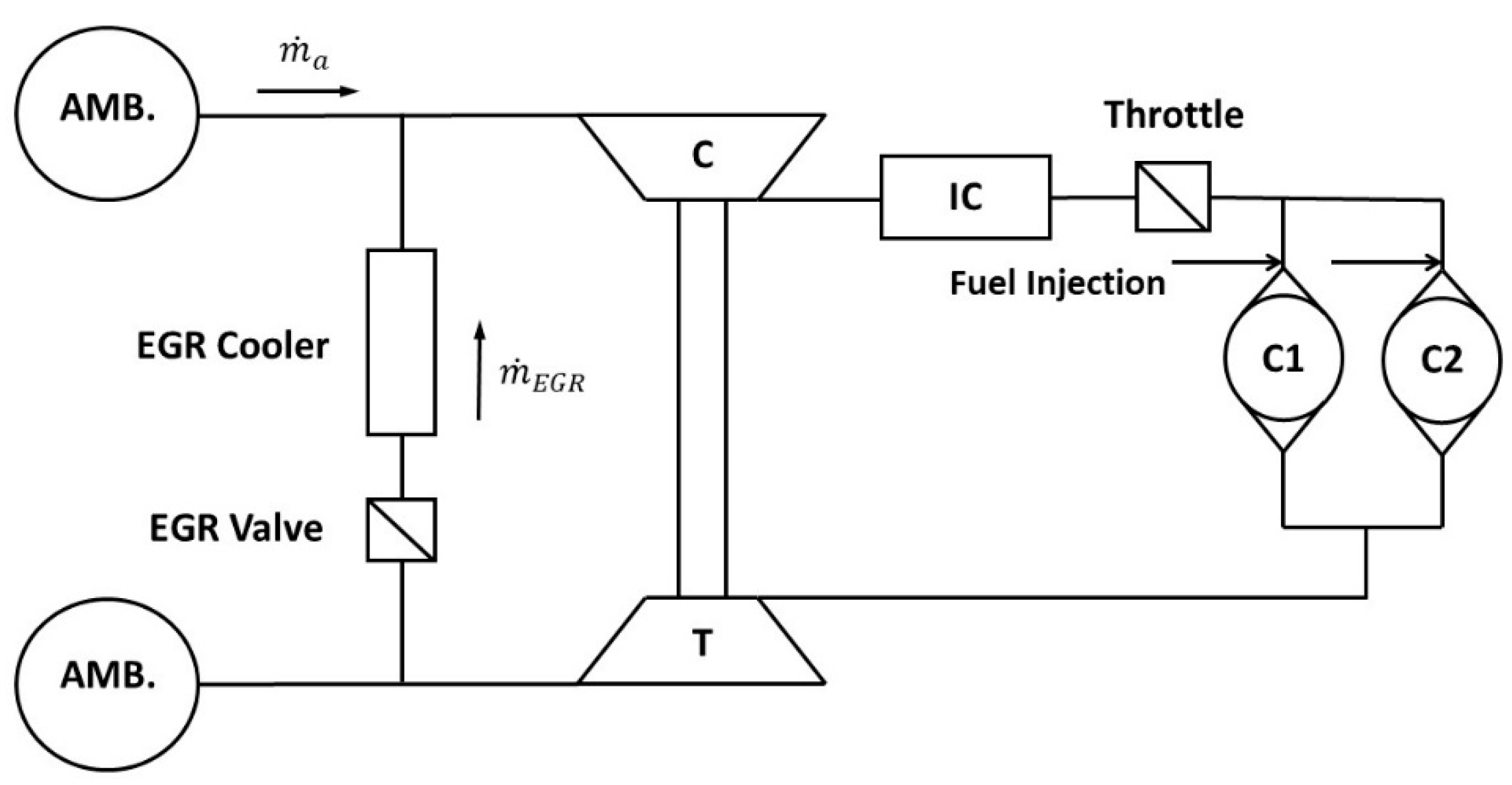
The engine is designed following the so-called “downsizing” concept. At high loads the engine works under knock-limited conditions and this requires to delay the combustion phasing (50% of mass fraction burned—MFB 50%), especially at lower speeds where a higher knock tendency usually occurs. On the other hand, at high speeds the A/F mixture has to be particularly enriched to maintain the Temperature at Turbine Inlet below a certain maximum allowable level. These control strategies, although mandatory for the examined engine, greatly penalize the fuel consumption at high loads. For this reason, the base engine configuration is properly modified for research purpose through the installation of an external low-pressure (LP) exhaust gas recirculation (EGR) circuit as depicted in Figure 1.

EGR rate and temperature are controlled through the throttle EGR valve and the cooler device, respectively. An enhanced cooling system, requiring a water cooled heat exchanger, is utilized to cool down the recycled gas. The LP EGR system was preferred over a high-pressure (HP) device, because it allows to avoid the pressure fluctuations and the counter-flow within the EGR circuit, due to the turbocharger dumping effect.

As known, EGR is essentially considered for knock control purposes at high loads, although certain EGR-related efficiency advantages are also obtained at part loads, due to the engine de-throttling.

The engine at test bench is also equipped along the exhaust line with a Three-way Catalytic converter (TWC) to guarantee the pollutant emissions (HC, CO and NOx) abatement, provided that the air/fuel ratio window very close to the stoichiometric value is maintained.

The exhaust system was opportunely modified to extract a portion of the exhaust gas from a single cylinder. In particular, a thin metallic tube is inserted inside of the exhaust manifold, through a properly realized hole, and oriented towards the exhaust side of one cylinder. The internal end of the above tube is located very close the exhaust valves. In this way, the exhaust gases of the selected cylinder (Cyl #1 in the following) are extracted and externally derived to measure the individual cylinder-out noxious emissions.

3. Experimental Setup and Test Procedure

As aforementioned, the tested engine is provided by an electro-hydraulic variable valve actuation (VVA) device. In spite of the VVA potentials, in the experimental tests the load is adjusted only acting on the throttle valve opening or waste-gate valve opening, without modifying the intake valve lift profile which is set to the “Full Lift” configuration. The intake air is constantly supplied to the engine at 293 ± 1 K by an air conditioning unit. Each engine cylinder is equipped with piezo-quartz pressure transducer (accuracy of ±0.1%) to detect the in-cylinder pressure signal.

The instantaneous pressure signals are acquired by the AVL INDICOM over 270 consecutive pressure cycles for the combustion analysis, assuming a polytropic thermodynamic process. A resolution of 0.1 CAD within the angular window between −90 and 90 CAD AFTDC is chosen, while outside this angular interval the sampling resolution is set at 1 CAD.

An automatic post-processing tool, based on a thermodynamic model, computes the ensemble averages of in-cylinder pressure and burn rate profiles and the combustion characteristics data. Furthermore, the boost pressure and the upstream turbine pressure are acquired through piezo-resistive low pressure indicating sensors located at the compressor outlet and at the outlet of the exhaust manifold, respectively. The engine is also equipped with thermocouples to monitor intake and exhaust temperatures, with particular attention to the control of the turbine inlet temperature in order to avoid unacceptable levels for the turbine blades.

A prototype driver, managed within LabView environment, is capable to switch from the commercial ECU to an external user control of the main engine variables: fuel injection timing and duration, boost pressure, spark timing, external EGR flow and temperature. EGR-related variables are managed acting on valve opening and cooler device within the EGR circuit.

Exhaust gas emissions are sampled upstream of the three-way catalyst. An ultra-violet gas analyzer (ABB UV Limas 11) measures NO_x. A cold extractive IR gas analyzer (ABB URAS) detects CO, CO₂ and O₂ while a FID analyzer (Siemens, Milano, Italy) is used for THC. A non-dispersive infrared sensor measures the CO₂ concentration at the inlet, downstream of the throttle valve to monitor the EGR rate. The sensor error is set at 0.07% for the measured CO₂ concentration.

The engine is tested in steady-state conditions at two different speeds (1800 and 3000 rpm) and various loads (from low to medium/high levels), also including increasing external EGR rates. In particular, EGR is modified by keeping constant the engine IMEP and the relative A/F ratio, λ. This means that at increasing the EGR rate the IMEP is restored to the nominal value with engine boosting; in a similar way, λ is maintained to the stoichiometric value by a modulation of gasoline injection duration. These operating points are selected because they are representative of the WLTC cycle for a segment A vehicle equipped with the engine under investigation. Performance in these points, such as fuel consumption and CO₂ emissions, are relevant for the vehicle homologation. Various operating parameters are collected during the experiments, including torque/power, air flow rate, fuel flow rate, boost and exhaust pressures and temperatures, exhaust emissions, etc.

The overall considered operating conditions are reported in

Table 2. Overall set of experimental engine points.

Load	Speed, rpm	IMEP, bar	λ, -	EGR Rate,%	SA, CAD AFTDC	Label
Low	3000	6.96	1.01	0.0	−30	3000@7
	3000	6.93	1.01	5.8	−38
	3000	6.92	0.99	9.0	−40
	3000	7.00	1.00	11.2	−45
	3000	7.02	1.01	14.9	−48
Med	1800	7.98	1.00	0.0	−20	1800@8
	1800	8.00	1.00	5.6	−27
	1800	8.07	1.00	10.0	−31
	1800	8.04	1.00	13.5	−31
	3000	9.05	1.00	0.0	−25	3000@9
	3000	9.04	1.00	5.4	−25
	3000	9.05	0.99	8.6	−30
	3000	9.00	0.99	16.2	−45
	3000	9.16	1.00	19.3	−50
	1800	10.08	1.00	0.0	−10	1800@10
	1800	10.04	1.00	5.3	−15
	1800	10.03	1.00	9.4	−21
	1800	9.96	1.00	14.4	−31
	3000	10.02	1.00	0.0	−16	3000@10
	3000	10.05	1.00	5.6	−21
	3000	10.16	1.00	14.6	−36
Med	3000	10.99	1.00	0.0	−14	3000@11
	3000	11.09	1.00	4.9	−18
	3000	11.08	1.00	7.7	−22
	3000	11.11	1.00	10.7	−26
	3000	11.04	1.00	15.7	−35
	3000	11.01	1.00	19.8	−50
Med/High	3000	13.10	1.00	0.0	−19	3000@13
	3000	13.12	1.01	6.4	−22
	3000	13.02	0.99	10.0	−26
	3000	13.07	0.99	14.6	−33

. Test grid collects 31 points which were gathered into 7 groups, each one characterized by the same nominal load level and rotational speed. For a single group, a label is defined (Table 2), referring to the nominal net IMEP and speed, which is utilized in the following figures. The table also shows the measured values of EGR rate, relative A/F ratio, λ, and the spark advance (SA). This last is selected to realize the Maximum Brake Torque (MBT) condition at knock free operations, while at high/medium loads the SA is chosen to operate at knock borderline (knock limited spark advance, KLSA). In particular, knocking is monitored by a knock sensor, installed between the two cylinders on the block, which automatically cuts out the power output and avoids the engine operation under severe knock conditions.

The measured net IMEP (Table 2) is properly derived from the acquired in-cylinder pressure traces over the entire engine cycle and represents the difference between the gross IMEP (in-cylinder pressure over compression and expansion strokes) and the pumping mean effective pressure (PMEP), evaluated over the intake and exhaust strokes.

Further parameters are monitored to preserve the safety of the turbocharger and of the entire engine. In particular, the boost pressure is controlled at high loads, acting on the waste-gate (WG) valve opening, to provide proper operation for the port injectors and to avoid the mechanical failures for the intake manifold. The average maximum in-cylinder pressure is constrained to limit the engine mechanical stresses. The mechanical and thermal safety of the turbine also obliges to control the turbocharger speed and the turbine inlet temperature (TIT). Summarizing, the following constraints are taken into account:

• Boost pressure: below 2.4 bar;
• TIT: below 950 °C;
• In-cylinder pressure peak: below 85 bar;
• Turbocharger speed: below 255,000 rpm.

4. Experimental Results

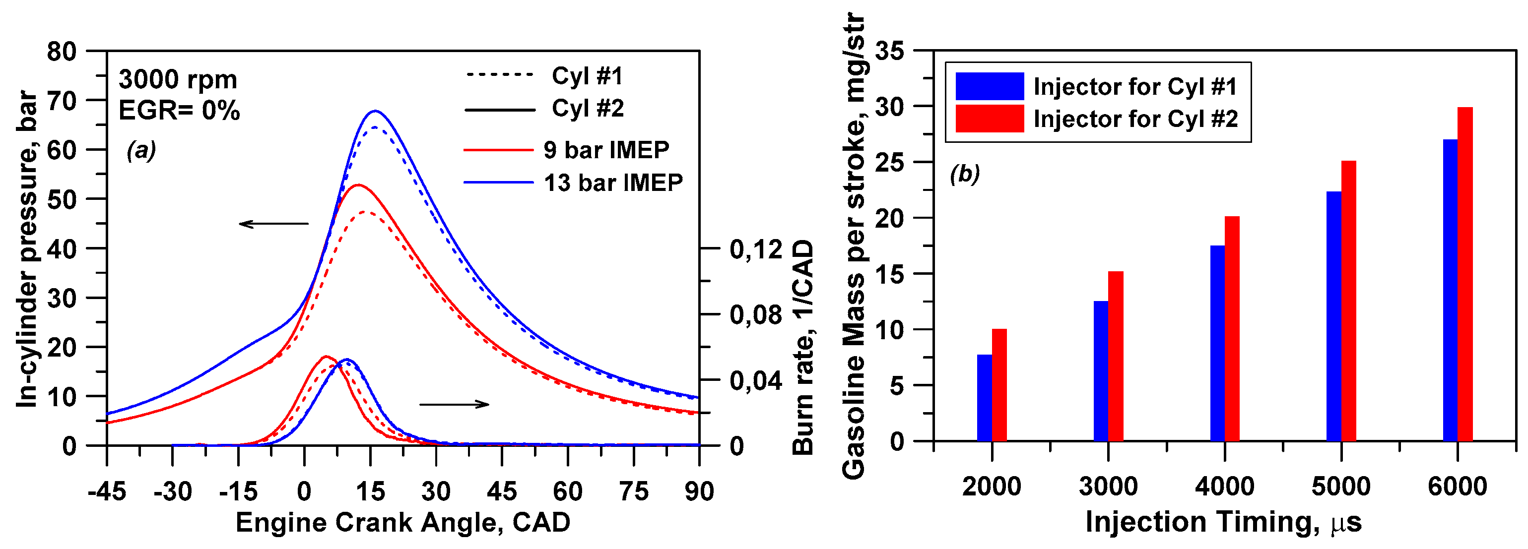
As discussed in the introduction section, experiments carried out on the examined engine have highlighted significant differences in the combustion evolution between cylinders, mainly ascribed to a non-uniform effective in-cylinder air/fuel (A/F) ratio [15]. Cylinder-by-cylinder variations are apparent in Figure 2a which shows the experimental in-cylinder pressure trace and the rate of heat release (ROHR) for two representative operating points (3000@9 and 3000@13, 0% EGR). As aforementioned, the pressure data refer to the ensemble average over 270 consecutive cycles. For both operating conditions, the pressure curves of two cylinders are overlapped in the compression stage, denoting the same air volumetric efficiency, while Cyl #2 provides higher pressure peak and combustion rate than Cyl #1. The same behavior is found at each investigated operating point, suggesting a systematic difference in pressure cycles. Further experimental tests on the adopted fuel injection system have highlighted a different fuel supply to cylinders, resulting from a variation in port injectors fuel rates (Figure 2b). The results plotted in Figure 2b were collected through injection tests realized at am-bent air pressure with fuel injection system removed from the engine. A drive signal to injectors was used to simulate the injection timing; a certain number of injection timings were considered to measure the gasoline mass per stroke delivered by injectors. In particular, consistently with the in-cylinder pressure traces shown in Figure 2a, the injector corresponding to Cyl #2 provides a higher fuel mass flow rate. Interestingly, no difference was found also when the relative position of two injectors was switched, indicating the fuel rail geometry as responsible of the cylinder-by-cylinder variation. Indeed, the gasoline rail mounted on the examined engine at test bench represents a non-optimized prototype geometry. The optimized version of rail, mounted on the commercial SI engine, does not exhibit differences in the gasoline mass flow rates between port injectors. All the previous considerations underline that rail geometry is main responsible for the experimental cylinder-by-cylinder variation analyzed in this research activity.

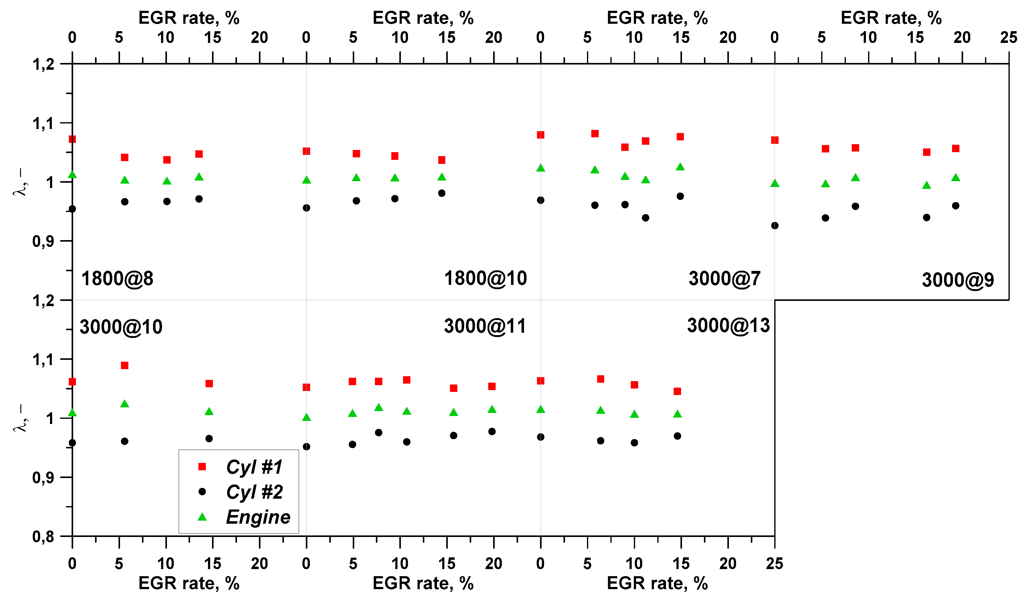
Figure 3 shows the relative air–fuel ratio (λ) in Cyl #1, Cyl #2 and the engine exhaust at different engine operating points and EGR rates. λ of Cyl #1 was estimated from the composition of the exhaust gases of that cylinder through the carbon balance of species. Similarly, the overall engine λ was verified from the overall exhaust gas composition. This allows to indirectly evaluate the λ value of Cyl #2 under the hypothesis of an equal volumetric efficiency for both cylinders, as suggested by the comparison of pressure traces in the compression stage. Even though the engine conditions are close to stoichiometric, lean (λ between 1.03 and 1.08) and rich (λ between 0.96 and 0.98) mixtures are obtained in Cyl #1 and Cyl #2, respectively. Considering that the engine does not provide an individual set of injection and combustion phasing for each cylinder, the same spark advance and injection parameters are chosen for both cylinders, optimizing the engine load. As a consequence, a difference in the single cylinder load is found at each operating condition.

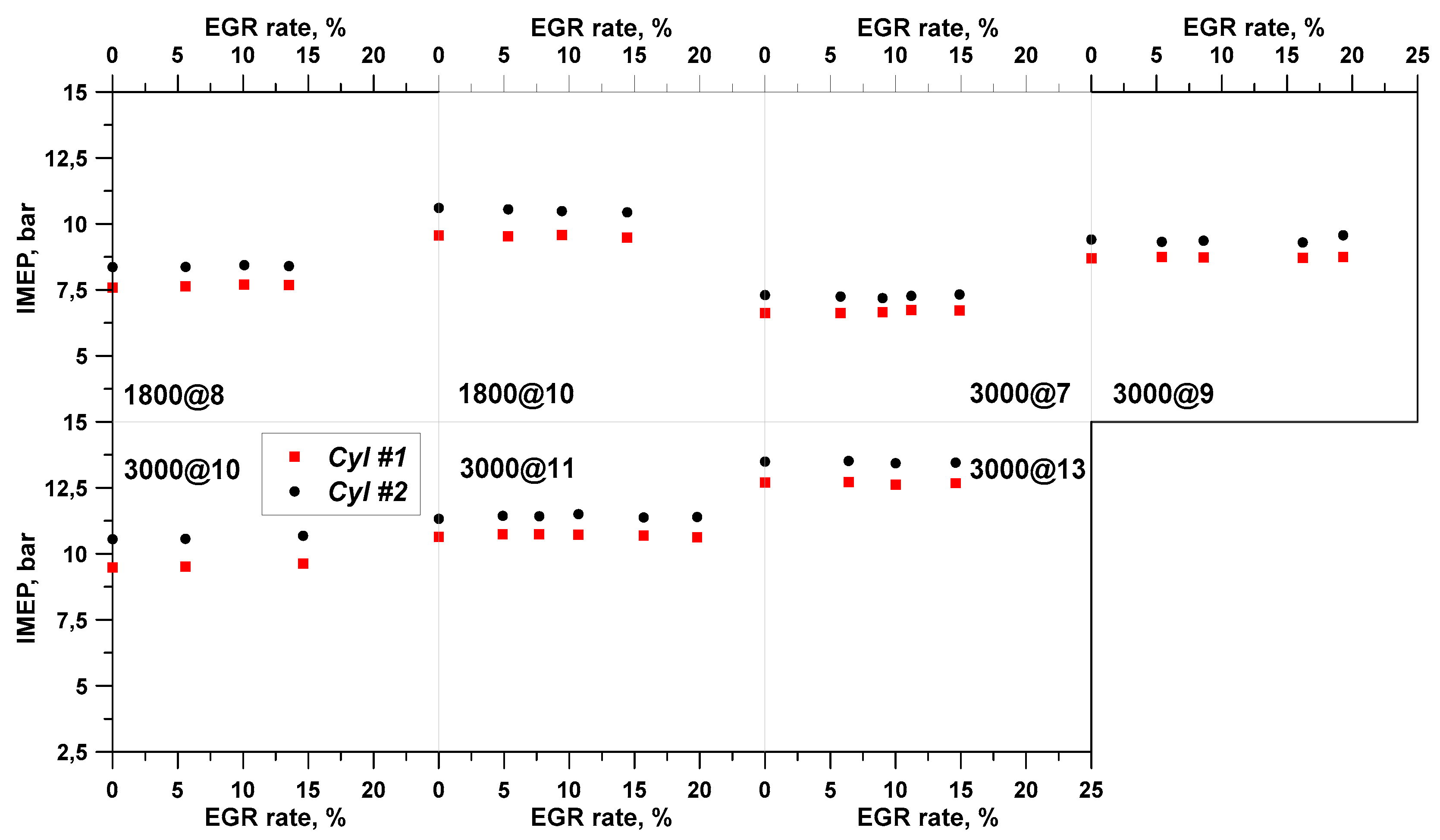
The individual IMEP levels for both cylinders at different operating points are shown in Figure 4 as a function of the EGR rate. As expected, the larger fuel amount introduced in the Cyl #2 results in a higher IMEP at each investigated condition. Furthermore, the adoption of the same spark advance for both cylinders penalizes the combustion phasing of Cyl #1 which results slightly late compared to the MBT. As concerns the trend versus the EGR rate, it is worth noting that the measurements are performed keeping constant the overall engine load; hence, the single cylinder IMEPs are almost constant at varying the exhaust-gas recirculation.

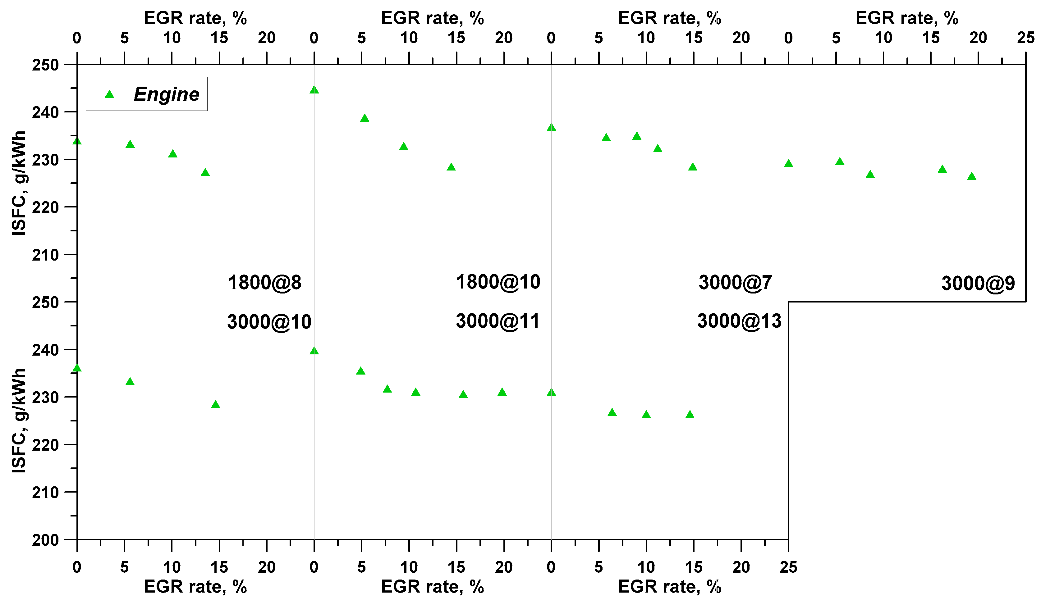
In Figure 5, the EGR-related trend of the engine ISFC is presented for the measured operating points. As expected, a reduced ISFC is observed at low and medium/high IMEPs by increasing the EGR content. At low loads, the ISFC benefits are ascribed to the EGR-induced reduction in the pumping losses promoted by the engine de-throttling; at medium/high loads, the ISFC advantages are obtained thanks to the EGR capability in reducing the knock tendency [18].

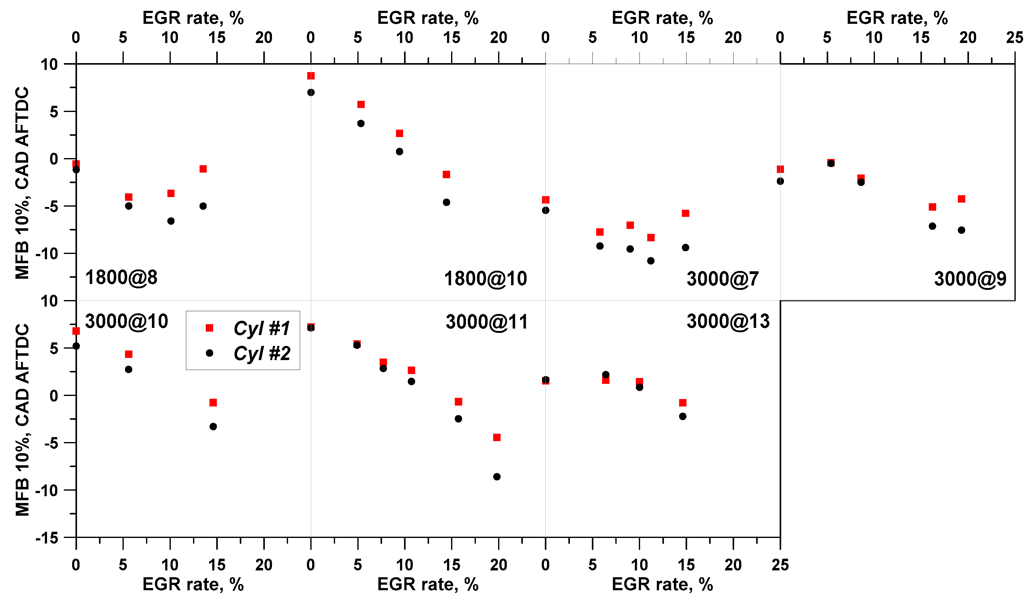
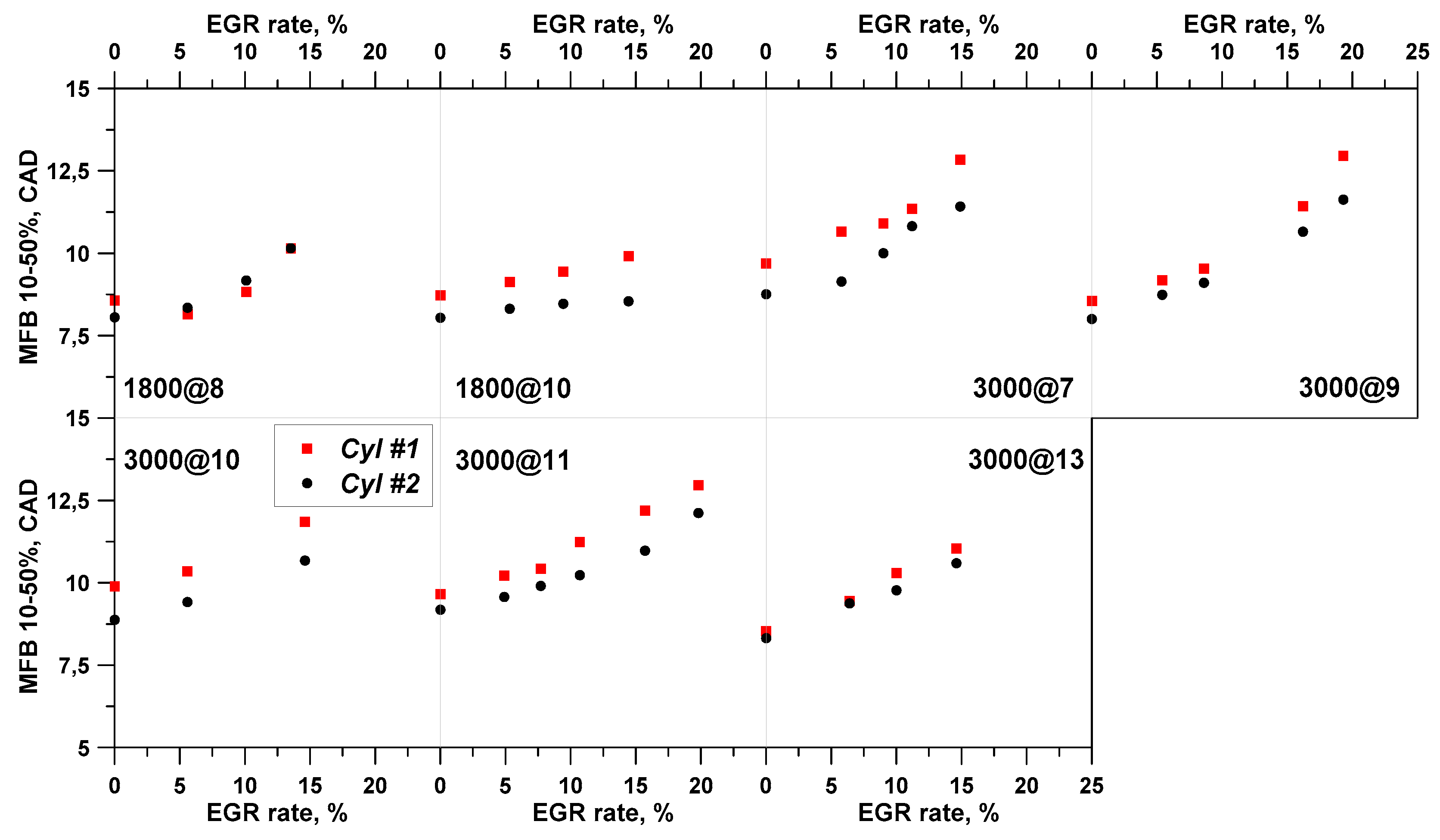
Figure 6 and Figure 7 show the characteristic angle of MFB 10% and the combustion core duration (MFB 10–50%) for both cylinders at different operating conditions. Looking at the early stage of combustion, at each operating condition, a slight delay in MFB 10% (Figure 6) of Cyl #1 compared to Cyl #2 is evident: the richer mixture in Cyl #2 provides a higher flame speed, advancing the MFB 10%. As shown in Figure 6, this gap increases at higher EGR rates; as is well-known, the charge dilution slows down the combustion rate, enhancing the effect of the equivalence ratio on the flame speed. The cylinder-to-cylinder variation in MFB 10% does not provide significant differences in the core combustion duration as reported in Figure 7. Even though the combustion duration in Cyl #1 results always prolonged compared to Cyl #2, the maximum difference in MFB 10–50% is less than 1.5 CAD at 1800@10 with 14.4% of external EGR. Regarding the effect of charge dilution on the combustion duration, the EGR prolongs the MFB 10–50% at each operating condition. This trend is more evident at higher engine speed, due to the reduction in cycle length, leaving a shorter period available to complete the combustion process. Further increase in combustion duration against the EGR is found at lower engine load, because of the greater impact of internal EGR which contributes to increase the overall in-cylinder residual content at decreasing the load.

5. Description of Modeling Approach

The engine used in this paper is outlined in a 1D model by employing the GT-Power commercial code. The whole engine is represented in sub-components, including cylinders, intake/exhaust pipes and turbocharging system. In particular, the flow inside the intake/exhaust ducts is reproduced by solving the conservation equations of mass (1), energy (2) and momentum (3) reported below:

dm/dt = Σṁ,

(1)

d(m·e)/dt = −p·dV/dt + Σ(ṁh) − dQ_w/dt,

(2)

dm/dt = {−dp·A + Σ(ṁ·u) − 4·C_f·ρ·u·|u|·A·dx/2·D − A·C_p·ρ·u·|u|/2}/dx,

(3)

where ṁ, m, V, p, e, h and u are mass flow rate, mass, volume, pressure, internal energy per unit mass, enthalpy per unit mass and velocity at boundary. Q_w is the heat exchanged through the walls, A is the flow area, D is the equivalent diameter. C_p and C_f are the pressure and friction losses coefficients, while dx and dp represent the discretization length and the pressure differential across dx. Each cylinder is treated as a 0D volume. In this case, the scalar variables (e.g., pressure, temperature, internal energy, etc.) are assumed to be uniform over the volume. However, during the combustion process the cylinder volume is divided in two zones (burned and unburned regions), where the mass and energy conservation equations are solved. In the closed valve period of single cylinder (i.e., from IVC up to EVO), the energy equation is detailed for burned and unburned zones as reported by relations (4) and (5):

d(m_u·e_u)/dt = −p·dV_u/dt − dQ_w,u/dt − h_u·dm_b/dt,

(4)

d(m_b·e_b)/dt = −p·dV_b/dt − dQ_w,b/dt + h_u·dm_b/dt,

(5)

where dm_b/dt represents the burning rate term evaluated through the turbulent combustion sub-model discussed in the following.

The turbocharging operation is simulated by a “map-based” approach. Turbine and compressor maps, supplied by the manufacturer, are employed within the standard turbine and compressor objects, respectively. Flow permeability of the single cylinder head is taken into account through the measured steady flow coefficients, both under forward and reverse flow conditions. Standard injector objects, available in the 1D code, are adopted for gasoline injection. During port injections, it is assumed that 30% of the total liquid mass vaporizes immediately upon the injection event, as advised for a typical liquid injector in GT-Power user manual; details about the spray evolution and wall film formation are not taken into account. In order to enhance the model capability, it is integrated with refined phenomenological in-cylinder sub-models of turbulence, combustion, heat transfer and pollutant emissions. A detailed description of these sub-models is reported in the next subsection.

5.1. In-Cylinder Sub-Models and Tuning: Combustion, Turbulence and Pollutant Emissions

In-cylinder 0D sub-models were integrated within the 1D engine model to refine the prediction of turbulent combustion and of the exhaust emissions. The combustion process is modeled by the fractal approach [19,20,21], where the burning rate is written as follows:

dm_b/dt = ρ_u·S_L·A_T = ρ_u·S_L·A_L·(L_max/L_min)^(D₃−2),

(6)

where ρ_u is the unburned gas density, A_L and A_T the area of the laminar and turbulent flame fronts, respectively, and S_L the laminar flame speed (LFS). L_min and L_max are the minimum and maximum flame wrinkling scales and D₃ is the fractal dimension. L_min represents the Kolmogorov scale evaluated under the hypothesis of isotropic turbulence, while L_max is proportional to a characteristic dimension of the flame front, i.e., the flame radius in the present study. D₃ is computed by the equation proposed in Reference [22], as a function of the ratio between the in-cylinder turbulence intensity and LFS. The latter is evaluated by using an “in-house” developed correlation, based on 1D LFS computations via chemical kinetics solver (CANTERA), accounting for the in-cylinder thermodynamic state (pressure p and temperature T), equivalence ratio, Φ, and EGR dilution. In particular, the adopted correlation reported in Equation (7) presents the well-known expression of the power law:

S_L = S_L0 ·(T/T_ref)^α·(p/p_ref)^β·EGR_factor,

(7)

In Equation (7), S_L0 is the flame speed at reference conditions T = T_ref and p = p_ref, depending on the fuel sensitivity S = RON-MON and Φ; EGR_factor is a reduction term for LFS that accounts for the presence of residual gas in the unburned mixture. Exponent α depends on Φ, T and p, while exponent β includes the dependencies on Φ and S. It is the case to underline that the above LFS correlation was developed considering a maximum EGR percent mass of 20%; therefore, the employed LFS correlation shows the capability to cover the range of examined EGR rates during the experiments (Table 2). The laminar flame area, A_L, is computed by an automatic procedure implemented in a CAD software and processing the actual 3D geometry of the combustion chamber. The estimation of L_min, and D₃ is based on the K–k–T turbulence sub-model, extensively reported in Reference [23]. The governing equations for the mean flow kinetic energy, K, the turbulent kinetic energy, k, and the tumble momentum, T_m, are as follows:

d(m·K)/dt = (ṁ·K)_inc − (ṁ·K)_out − f_d·m·K/t_Tum + m·K·ῤ/ρ − P,

(8)

d(mk)/dt = (ṁ·k)_inc − (ṁ·k)_out + (2·ῤ/3·ρ)·(m·k − m·υ_t·ῤ/ρ) + P − m·ε,

(9)

d(m·T_m)/dt = (ṁ·T_m)_inc − (ṁ·T_m)_out − f_d·m·T_m/t_Tum,

(10)

In Equations (8)–(10), the first and second terms describe the incoming and the outcoming convective flows through the valves, respectively. The third term for the K and T_m equations is the decay contribution due to the shear stresses with the combustion chamber walls by means of the decay function, f_d, and the characteristic time scale, t_Tum. In Equation (9), third term represents an additive compressibility term, proportional to (ῤ/ρ); the latter is also included in the K equation as the 0fourth term. P describes the energy cascade mechanism, which causes the transfer of kinetic energy from the mean flow to the turbulent flow. Finally, the last term in Equation (9) takes into account the viscous dissipation rate of k into heat. The described turbulence sub-model proved to be able to adequately reproduce the in-cylinder turbulence evolution along the whole engine cycle, also sensing the variations in the engine operating conditions, the valve strategies and the cylinder geometrical parameters [23]. The heat-transfer model both for cylinders and exhaust subsystem is considered, applying a wall temperature solver based on a finite element (FE) approach. For the in-cylinder heat transfer (gas-to-wall), the Hohenberg correlation is implemented into the 1D code while convective, conductive and radiative heat transfer modes are considered for the exhaust pipes. The Hohenberg correlation here utilized is illustrated in Equation (11):

H = A·V ^−0.06·p ^0.8·T ^−0.4·(v_pm + B) ^0.8,

(11)

where V is the volume, p is the pressure, T is the mean gas temperature and v_pm is the mean piston speed. The calibration constants, A and B, are calculated by Hohenberg and here used as 130 and 1.4, respectively. The convective heat transfer coefficients for engine coolants (oil and water) are evaluated by simulations of coolant circuits. They are subsequently imposed as an input in the code, assuming a dependency on the engine speed. Cooling boundary conditions (temperatures for oil and water) are introduced in the model according to the levels recommended by the engine manufacturer. Concerning the model tuning, an integrated 3D/1D approach is adopted for turbulence sub-model [23]; model constants are identified to better reproduce the turbulence outcomes of in-cylinder 3D CFD simulations, under motored conditions and for various speeds and valve strategies [23]. Referring to the combustion model tuning, this sub-model includes three tuning constants differently affecting the distinct phases of combustion process. A single set of tuning constants was identified for the considered operating points, and tuning is kept fixed regardless the engine operating conditions. A particular attention is devoted to the modeling of the pollutant emissions. To this aim, “in-house developed” sub-models for the estimation of the main regulated cylinder-out emissions, namely HC, CO and thermal NO, are implemented into the 1D code. The propagation of the cylinder-out noxious species within the exhaust system up to the inlet section of TWC is also considered in the 1D model. In particular, CO concentrations are computed by solving, in the burned gas zone, a simplified chemical kinetic sub-model based on two-step reactions as reported in Reference [24]. The CO mechanism comprises the following high-temperature CO oxidation reactions (12) and (13):

CO + OH ↔ CO₂ + H,

(12)

CO + O₂ ↔ CO₂ + O,

(13)

For thermal NO emission, a refined approach is here adopted, where the semi-detailed chemical kinetics scheme proposed by Andrae [25] is applied to the burned gas zone to compute the NO concentrations in each cylinder. The kinetic mechanism includes 5 elements, 185 species and 937 reactions. This methodology, although computationally more expensive than the classic Zeldovich scheme, seems to be better in predicting the NO emissions of the single cylinder at varying the thermodynamic conditions, including pressure, temperature, inert content and mixture quality. HC production is simulated by the crevices model and a wall-flame quenching correlation, combined with a thermal-based HC oxidization equation during the expansion stroke. This means that the mixing-based oxidation contribution is neglected by assuming a perfect and instantaneous mixing of unburned charge from crevices with the hot burned gases. In the filling/emptying crevices model, HC species are assumed to accumulate/be released during the in-cylinder pressure rise/decrease phase in/from an arbitrary assigned constant volume, V_crev, as a fraction of the combustion chamber volume at TDC [26]:

x_crev, % = 100·V_crev/V_cyl-TDC,

(14)

The volume V_crev schematizes the crevices in the combustion chamber where the flame front extinguishes and it is controlled in the model by the input parameter, x_crev. The temperature in crevices volume is considered to be the same as the cylinder wall. A constant flow coefficient is attributed to the orifice of the crevices volume both for incoming and outgoing mass flows. Therefore, the pressure evolution within the crevice volume is computed by combining the related mass and gas temperature profiles. For the flame wall-quenching contribution, a simple correlation is here assumed which furnishes an estimation of the total HC arising from the extinguished flame at cylinder walls as a function of the flame quenching distance. This last parameter is assumed inversely proportional to the laminar flame speed, since the flame reaches the wall in laminar conditions. Flame quenching distance varies during the combustion evolution, and, in this study, it is taken towards the end of combustion process (i.e., 90% of mass fraction burned). Indeed, it is quite reasonable to assume that the HC generated by the flame-quenching during the initial combustion phase rapidly diffuse in the burned zone and oxidize. The correlation employed in this study for the quenching-related unburned HC resembles the simple model proposed in Reference [27], and it is shown in Equation (15):

HC_quench = H₁·δ_L + H₂,

(15)

where δ_L is the laminar flame thickness, while H₁ and H₂ are sub-model tuning constants. Finally, for the oxidation of the overall HC level during the expansion stroke the one-step kinetic equation proposed in Reference [28] is adopted. The rate of post-flame HC oxidation is computed according to Equation (16):

d[HC]/dt = −6.7 × 10¹⁵ × e^{−(18735/R·Thc)}·[HC]·[O₂] (p/R·T_hc)²,

(16)

This rate depends on the HC and molecular oxygen concentrations, the density term (p/RT_hc) and on the oxidation temperature, T_hc. The latter is computed as a weighted average between the in-cylinder mean gas temperature and the wall temperature.

5.2. Simulation Setup

Concerning the 1D model setup, at low loads, the experimental IMEP is reproduced by a Proportional-Integral-Derivative (PID) controller acting on the throttle (THR) valve opening, while the WG valve is fully opened. At high loads, the measured IMEP is obtained by another PID controller adjusting the WG valve opening and considering the fully opened throttle valve. In each operating condition, the injected fuel mass is monitored to reproduce the different experimental λ level for each cylinder. The experimental EGR rate is replicated by regulating the EGR valve opening with an additional PID controller. The spark advance is automatically modified in the cycle-by-cycle calculation to realize the measured combustion phasing (MFB 50%). The above-discussed model setup is taken into account in the numerical analysis, and the related outcomes are presented in the next section.

6. Numerical Analysis

The accuracy of the developed 1D engine model is proved for the entire set of measurements (Table 2). In a first stage, the model capability is tested in replicating the main performance variables such as the in-cylinder pressure peak and combustion core duration for both cylinders, the Indicated Specific Fuel Consumption (ISFC) and the Temperature at Turbine Inlet (TIT). A detailed analysis is also presented with the aim to demonstrate the model proficiency in reproducing the main gaseous emissions (NO, CO and HC). Particular care was paid to the numerical/experimental assessment of the single cylinder performance and emissions in order to reproduce the effect of cylinder-by-cylinder variation. In a second phase, the validated model is applied to evaluate the improvements in terms of ISFC and pollutant emissions resulting from the suppression of the cylinder-by-cylinder A/F ratio imbalance.

6.1. Model Validation

Referring to the performance parameters, the following figures, Figure 8, Figure 9 and Figure 10, report the numerical/experimental comparisons for the overall set of measured operating points, including the variations in load level, speed, EGR rate and cylinder-related air/fuel ratio. The figures also present the average absolute or percent error between the numerical and the experimental outcomes.

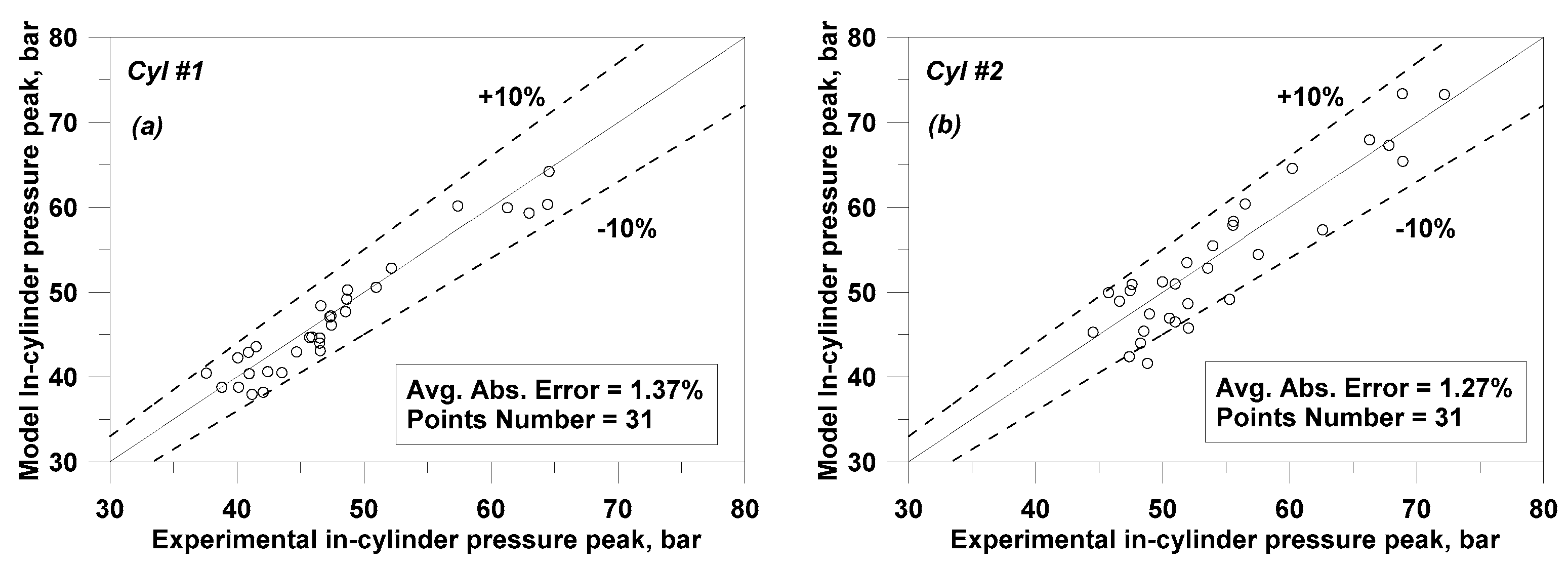
The results plotted in Figure 8a,b show that the model is capable to capture with similar accuracy the experimental pressure peak of both cylinders, denoting very limited absolute percent errors of numerical predictions. These assessments also highlight the good reliability of the combustion modeling for the individual cylinders.

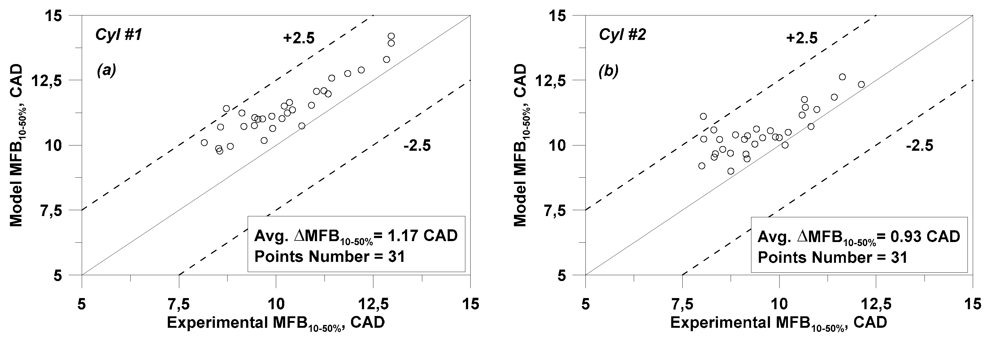
To further prove the model capability in reproducing the combustion process evolution, the numerical/experimental assessment of the combustion core duration (MFB 10–50%) is reported in Figure 9. Combustion duration of both engine cylinders is adequately described by the model, as demonstrated by the reduced average difference between predicted and experimental data (1.17 CAD and 0.93 CAD for Cyl #1 and Cyl #2, respectively). The above outcomes demonstrate the model ability to sense the effect of cylinder-by-cylinder differences in thermodynamic state (pressure and temperature), mixture quality and composition (A/F ratio and EGR content).

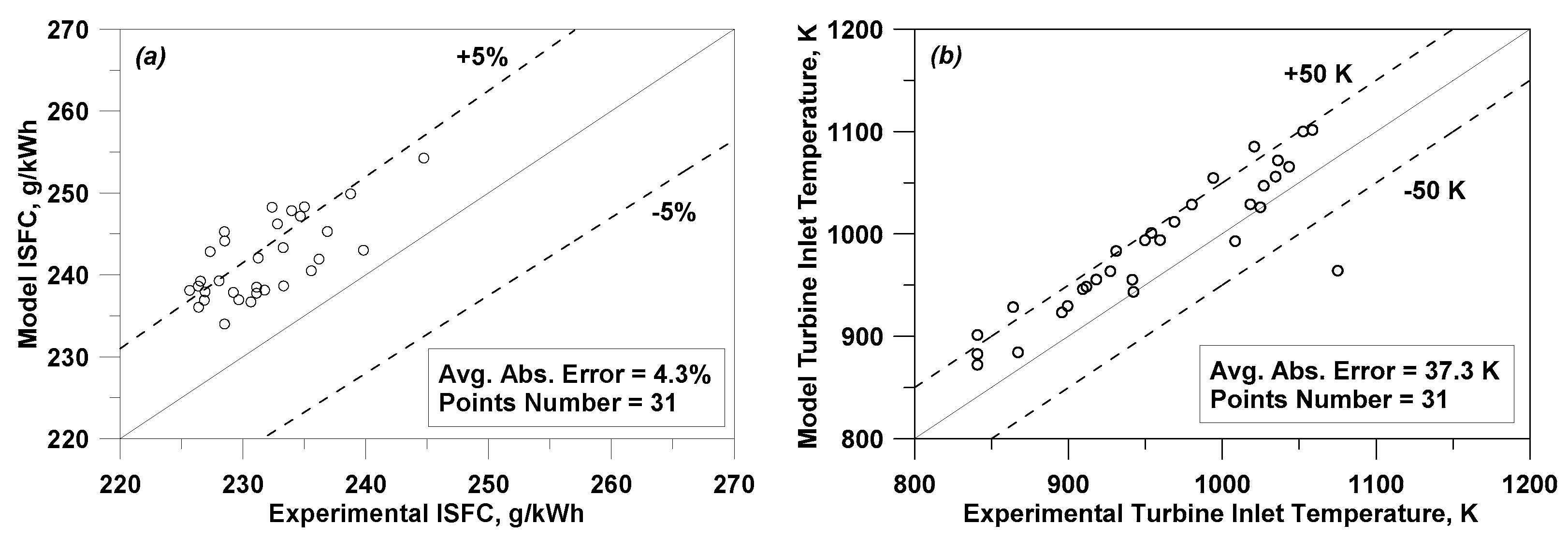
As a relevant global engine performance, Figure 10a presents the numerical/experimental assessment for the ISFC. A satisfactory correlation with the measurements is found for the overall data set with an average percent error of 4.3%. Greater ISFC differences are detected for points at speed of 1800 rpm, mainly due to the model overestimation of the air flow rate. ISFC errors are lower at speed of 3000 rpm. However, most of the computed points are included in the considered allowable error band ±5%, thus demonstrating an acceptable model capability for the ISFC prediction.

Good numerical/experimental agreements for TIT (Figure 10b) are reached, thanks to the refined thermal modeling, which also includes the FE approach for cylinders and exhaust pipes. Indeed, the computed TIT shows a good correlation with the experimental data (mean absolute temperature error of 37.3 K). Although not visible in Figure 10b, the model correctly reproduces the trend of TIT reduction at increasing the EGR rate and lowering the IMEP.

Even if not reported here for brevity, the in-cylinder pressure traces and the other global performance variables are reproduced with accuracy similar to a previous authors’ work [15].

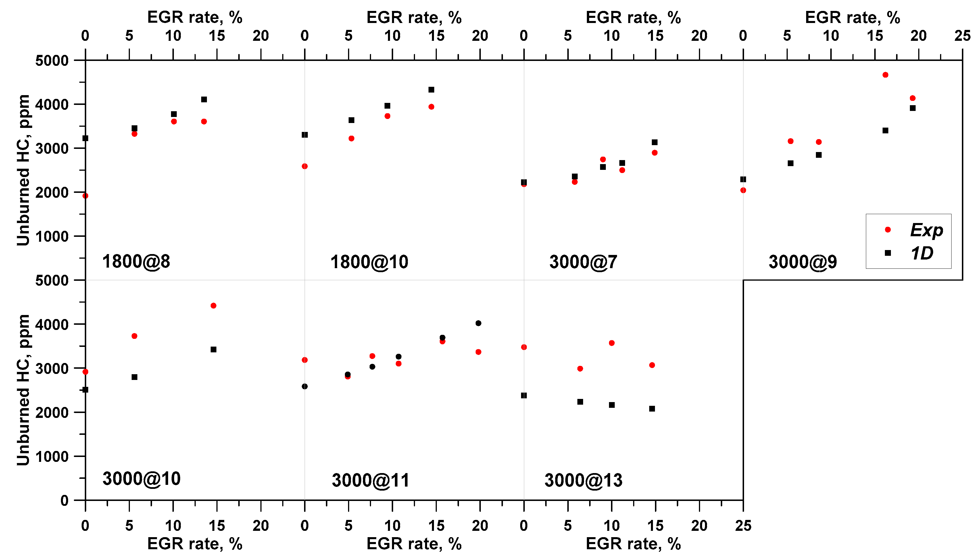
As for pollutants, Figure 11, Figure 12 and Figure 13 show the comparison between numerical and experimental levels of regulated gaseous emissions: NO, CO and HC, respectively. Consistently with the presentation of the experimental results, the variations of considered pollutant emissions are reported as a function of the EGR rate.

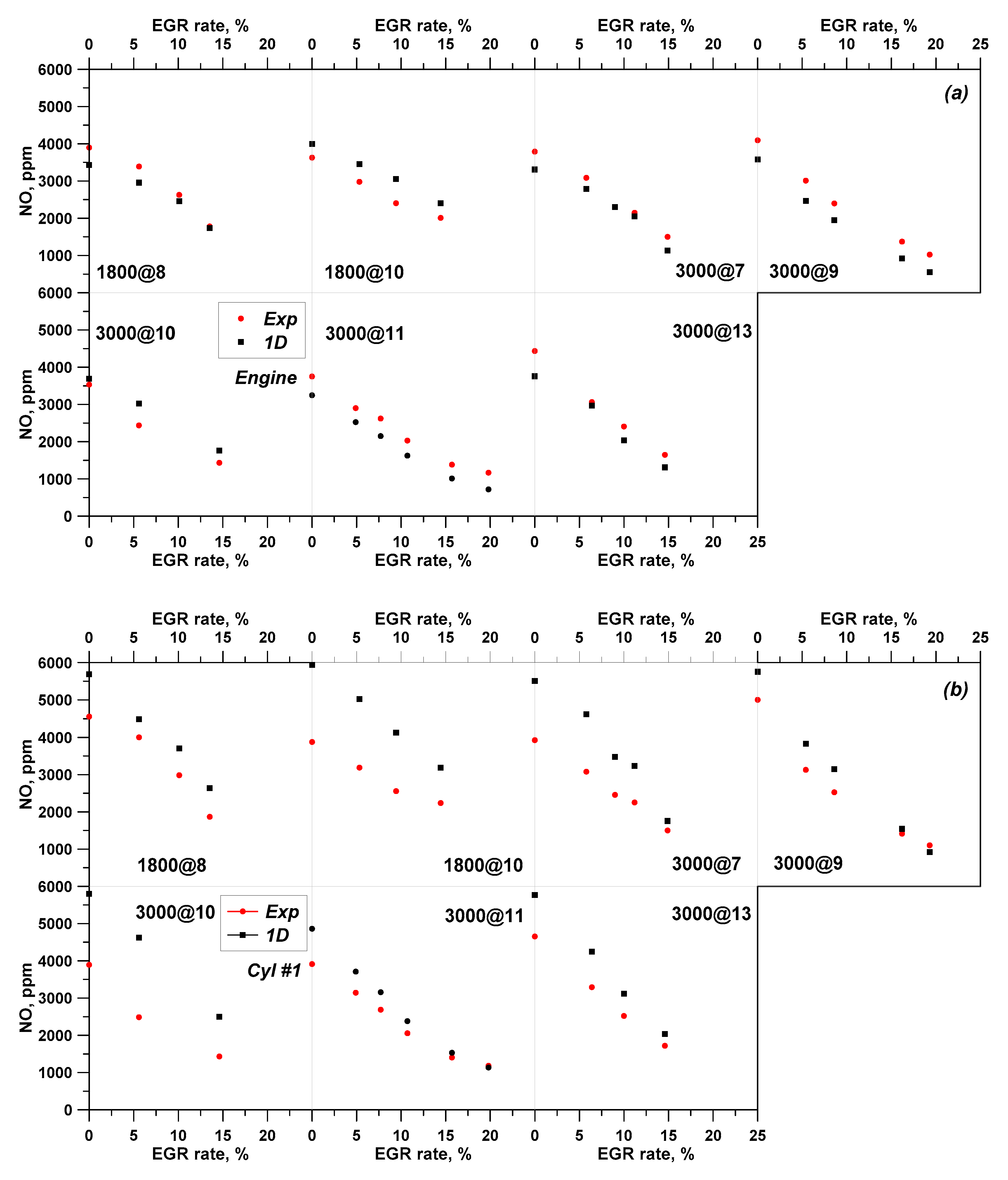
Figure 11a,b show the NO emissions at the engine exhaust (Figure 11a) and at the exit of exhaust valve of Cyl #1 (Figure 11b), at different points and EGR rates. At each investigated operating condition, engine NO emission decreases at increasing the EGR rate with a reduction between ~45% and ~55% at 1800 rpm and between ~60% and ~90% at 3000 rpm when the maximum charge dilution is adopted. Looking at Figure 11b, the Cyl #1 NO emission strongly increases compared to the overall level at the engine exhaust. This behavior can be explained considering the relevant difference in the A/F ratio of two cylinders: running the engine at stoichiometric conditions the relative A/F ratio in Cyl #1 ranges between ~1.03 and ~1.08 and the higher oxygen content speeds up the NO formation reactions. The comparison between experimental and numerical data demonstrates that the employed NO modeling approach is capable to adequately reproduce the EGR-induced trend of the NO emission reduction for both the single cylinder (Cyl #1—lean A/F ratio) and the engine exhaust (stoichiometric A/F ratio). Indeed, the NO sub-model correctly senses the formation mechanism, which is primarily affected by the in-cylinder temperature and by the presence of some species (CO₂, H₂O, N₂ and O₂) in the fresh air/fuel mixture [29].

The model demonstrates to well capture the level of the engine NO emissions (Figure 11a) even if a limited model underestimation (average error around 15%) is observed in most of the analyzed conditions. Conversely, greater errors in the prediction of NO emissions coming out of Cyl #1 are obtained (Figure 11b). In this case, the model average error in predicting the measured Cyl #1 NO emission is of about 30%. Indeed, higher differences between the computed NO emissions of Cyl #1 and of Engine are obtained by the model, when compared to the same experimental differences. This consideration highlights the prediction limitations of NO sub-model in the range of lean A/F mixtures, as in the case of Cyl #1. The numerical inaccuracies reported in Figure 11b may be probably attributed to the high sensitivity of NO sub-model to the relative air/fuel ratio variations.

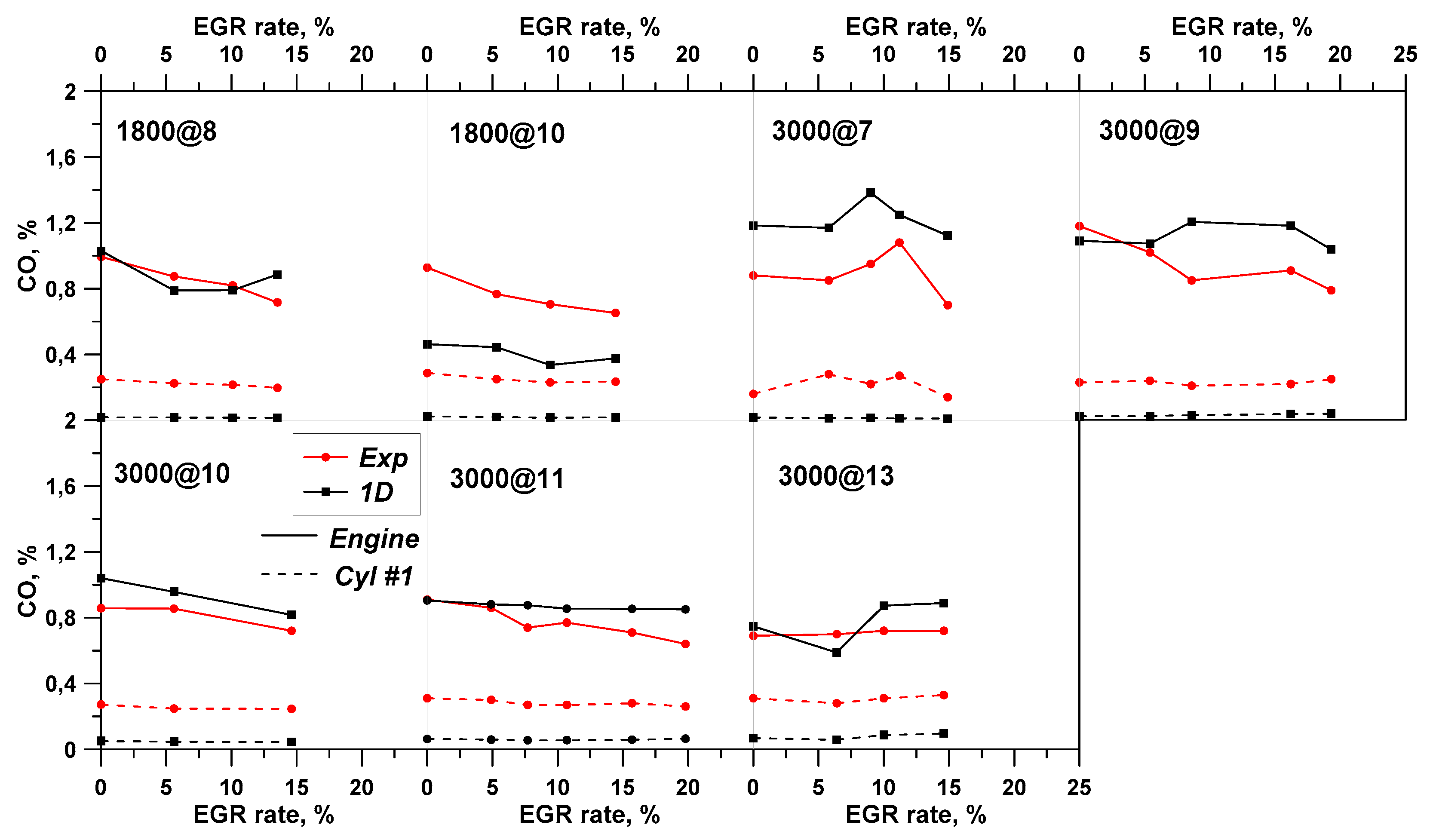
CO emissions are plotted in Figure 12, where a good prediction of the experimental values for both the engine and the Cyl #1 is obtained. Engine CO is reproduced by the model with an average error of about 30% over the tested operating conditions.

Very low CO emissions are measured for Cyl #1, because of lean mixture operations. The model systematically underestimates the CO levels for Cyl #1 at varying the EGR. This could be attributed to a model limitation which does not include the CO generated by the partial oxidation of unburned HC at the cylinder walls under lean conditions.

However, the experimental/numerical correlation of CO levels for Cyl #1 is taken as satisfactory, also considering the experimental errors in recording small emission levels. The outcomes in Figure 12 suggest that the numerical CO emissions of Cyl #2 are also reliable even if they cannot be compared to any measured data.

Figure 13 proposes the numerical/experimental assessment for the sole engine unburned HC emission. Unfortunately, the single cylinder HC data cannot be proposed here, because the Cyl #1 exhaust probe is located very close the exhaust valves, and, as clearly discussed in Reference [30], a relevant instantaneous peak of unburned HC emission is realized at the event of exhaust valve opening. This phenomenon involves some difficulties to furnish a reliable measure of the HC level for Cyl #1 with the available gas-emission analyzer.

According to Figure 13, the HC sub-model demonstrates to be able to reproduce the experimental trend of the engine unburned HC emissions at varying the EGR rate. In particular, the model provides an average error of 18% in the prediction of engine unburned HC species. Concerning the set of EGR-sweep operating points, only for the highest investigated IMEP (3000@13) a slight HC reduction is observed at increasing the EGR. As known, the engine load and A/F ratio are found to be the main parameters influencing the quenching phenomenon, through the quenching distance variations [27]. Since the quenching distance is proportional at first order to the laminar flame thickness, at increasing the IMEP the wall-flame quenching furnishes a gradually reduced in-cylinder HC production. It is very likely that, at 3000@13, the quenching exerts a limited impact on the HC emission. Therefore, at 3000@13, the EGR-related HC reduction has to be ascribed to the spark timing advance (Table 2). In addition, at 3000@13, the rise in boost pressure at increasing the EGR content, required to restore the engine IMEP, is more prominent than the other load conditions. This also means that higher temperature levels are expected to occur during the expansion phase, thus improving the HC post-oxidation and contributing to reduce its overall level.

For all the other points, higher HC emissions are obtained as the EGR rises, and the model well captures this trend, mainly thanks to the contribution of the wall flame quenching.

In light of the above-discussed results, the proposed modeling approach shows the capability to satisfactorily take into account the influence of both engine operation and cylinder-by-cylinder variations on the main pollutant emissions, without the need of a case-dependent tuning.

6.2. Model Application: Suppression of A/F Ratio Imbalance between Cylinders

Once validated, the model is utilized to evaluate the engine behavior in the case of the virtual suppression of the cylinder-by-cylinder variation. To this aim, the experimental A/F ratio imbalance between cylinders for the examined engine is removed and a stoichiometric A/F ratio is imposed in each cylinder, while preserving the measured combustion phasing as input data. As a consequence, variations in the performance and emissions of the engine are expected to occur and can be easily estimated. It is the case to underline that authors focused on showing the single effect related to the suppression of A/F ratio imbalance between cylinders. Of course, a more refined engine calibration also requires a control of combustion phasing to reach the optimal levels at both low and medium/high loads. The main numerical outcomes of the above-discussed investigation are plotted in the Figure 14 and Figure 15. In each figure, the 1D results obtained by imposing the measured A/F ratio for individual cylinder (labeled as “Unbalanced A/F ratio”) are compared with the 1D outcomes resulting from the imposition of a stoichiometric A/F ratio as input data for two cylinders (labeled as “Balanced Stoichiometric A/F ratio”).

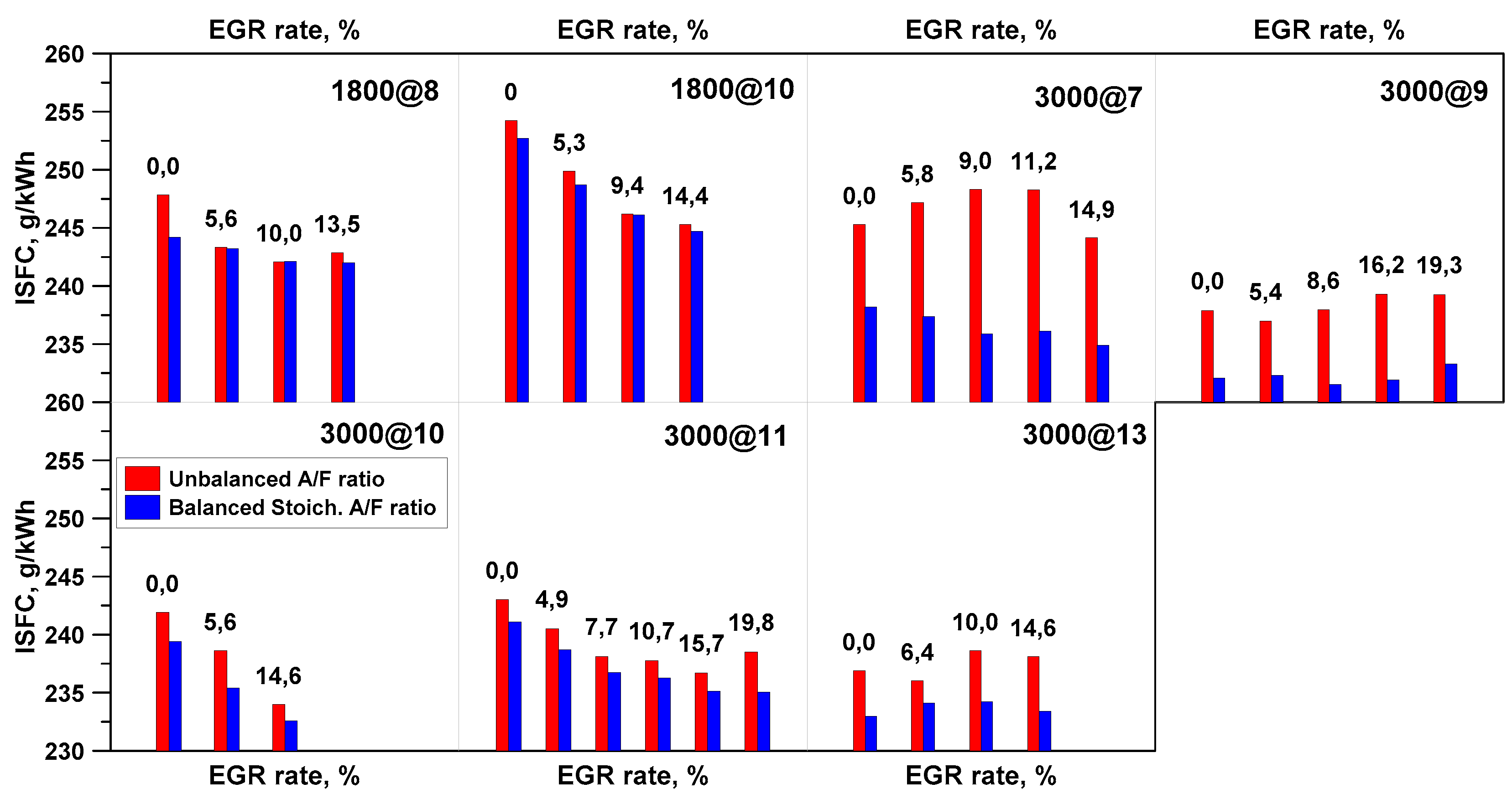
Figure 14 shows the ISFC comparisons in the analyzed engine operating points. Interestingly, this figure highlights that not negligible ISFC improvements are realized and the lower ISFC levels resulting from the balanced A/F ratio (blue bars in Figure 14) mostly follow the EGR related trend. A maximum ISFC percent benefit equal to 5% (ΔISFC = 12.4 g/kWh at 3000@7, EGR% = 9%) is attained, while the average percent gain is around 2%.

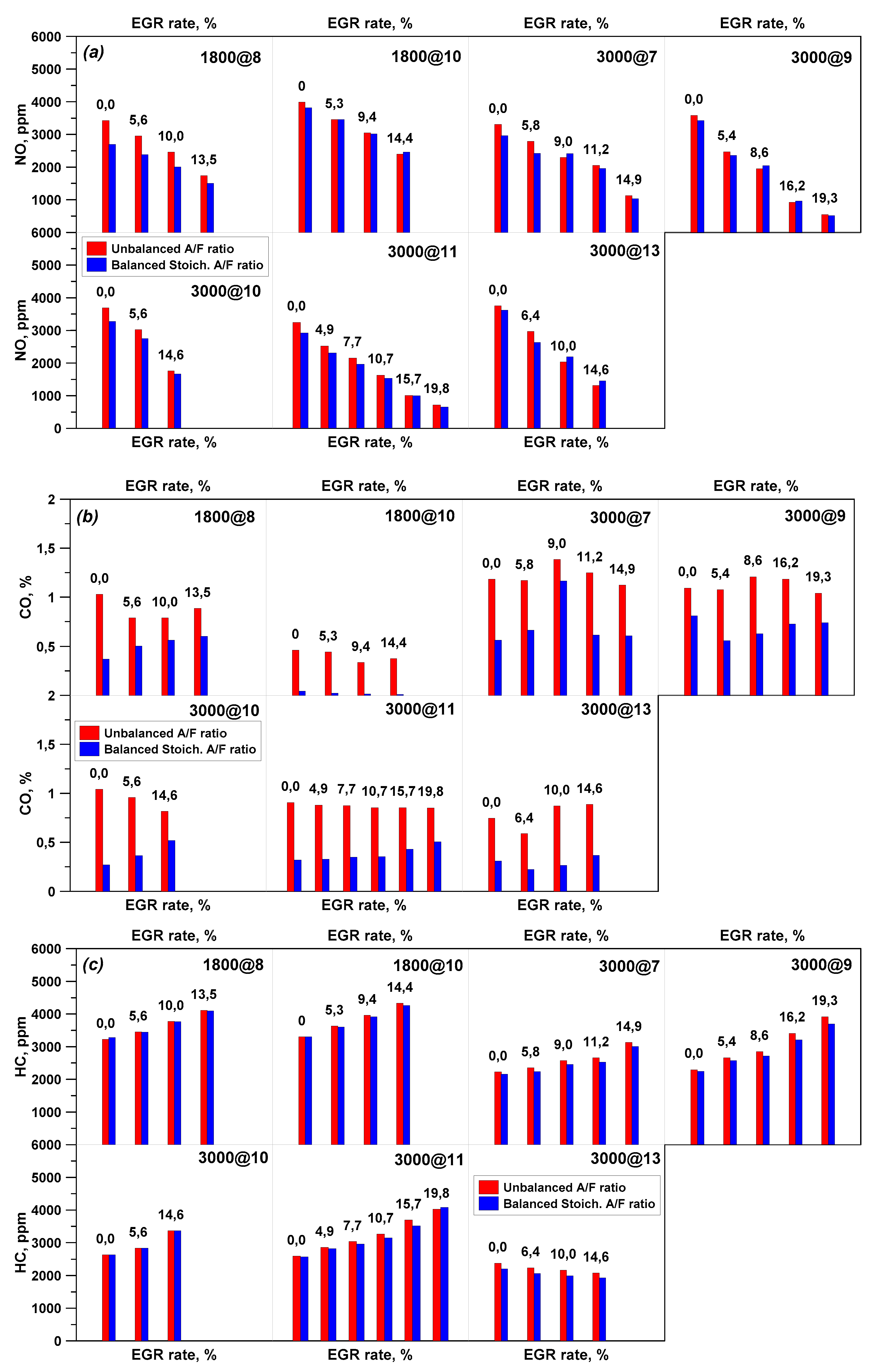
Referring to the main pollutants, the results plotted Figure 15a–c demonstrate that the cylinder-by-cylinder variation exerts a certain influence on both NO, CO and unburned HC emissions. CO improvements are substantially independent from the EGR variation (Figure 15b). The engine CO emission is strongly affected by the cylinder variability with a percent average reduction of about 50%. A peak of CO reduction (about 97%) is observed at 1800@10 and EGR% = 14.4% corresponding to an absolute ΔCO% of 0.36% (Figure 15b). Conversely, NO and unburned HC emissions exhibit reduced benefits (Figure 15a,c, respectively) and the optimized NO and HC species continue to follow the expected trend with EGR. The percent advantage for the HC emission reaches a peak of 8% (ΔHC = 171 ppm at 3000@13, EGR% = 10%) while the average benefit in HC emission is of 2.5%. Similar and only slightly greater benefits are observed for the NO emission: mean percent gain around 5% and peak advantage of 21% (ΔNO = 730 ppm at 1800@8 with EGR% = 0%). It is the worth to underline that the obtained advantages cannot be considered as a general case, but they should be taken as a prediction related to the analyzed engine and the measured points. Hence, the results illustrated in Figure 15 are solely related to the analyzed engine configuration and they lose their meaning in the case of mature commercial SI unit. As a final remark, a refined engine calibration which includes a control on both A/F ratio and combustion phasing can lead to further performance advantages, especially in terms of fuel consumption.

7. Conclusions

In this work, experimental and 1D numerical analyses were performed on a twin-cylinder turbocharged spark ignition engine with the aim to study the effects of cylinder-by-cylinder variation on performance, combustion and gaseous emissions.

In a first stage, experimental tests were carried out at different speed/load points and EGR rates. The experiments pointed out the following main results:

• The assessment of experimental pressure traces and the rates of heat release between cylinders suggests a systematic difference in fuel supply to cylinders, also confirmed by fuel rate difference of port injectors;
• The composition analysis of exhaust gas highlights two different mixture conditions for cylinders;
• Cylinder-by-cylinder λ variation involves a different response to EGR variation in the IMEPs and combustion evolutions between cylinders.

In a second step, a 1D engine model was realized in a commercial code and integrated with “users” in-cylinder sub-models to refine the description of turbulence, combustion, heat transfer and emissions.

Numerical study has pointed out the following main outcomes:

• Engine model satisfactorily reproduces the overall performance and combustion evolution of each cylinder at varying the operating conditions;
• Measured trends of main emissions (NO, CO and HC) for both engine and single cylinder are well captured by the model;
• Validated model is applied to quantify the improvements in terms of ISFC and main pollutants (NO, CO and HC) by suppressing the air/fuel ratio imbalance between cylinders over the examined points.

The wide numerical/experimental investigation of the influence of cylinder-by-cylinder variation on performance and emissions of a SI engine represents the novel contribution of this work compared to the existing literature analyses. The proposed modeling approach has the relevant benefit of a favorable compromise between the results accuracy and computational cost. It can be proficiently adopted to support the control and the design of a spark ignition engine for cylinder-by-cylinder variability suppression with the aim of improving performance and emissions.