Article

Different Formulations to Solve the Giesekus Model for Flow between Two Parallel Plates

by
Laison Junio da Silva Furlan
1,†,
Matheus Tozo de Araujo
1,†,
Analice Costacurta Brandi
2,
Daniel Onofre de Almeida Cruz
3 and
Leandro Franco de Souza
1,*
1
Department of Applied Mathematics and Statistics, University of Sao Paulo, Sao Carlos 13566-590, Brazil
2
Department of Mathematics and Computer Science, Sao Paulo State University, Presidente Prudente 19060-900, Brazil
3
Department of Mechanical Engineering, Federal University of Rio de Janeiro, Rio de Janeiro 21941-972, Brazil
*
Author to whom correspondence should be addressed.
These authors contributed equally to this work.
Submission received: 30 September 2021 / Revised: 19 October 2021 / Accepted: 21 October 2021 / Published: 28 October 2021

Abstract

:
This work presents different formulations to obtain the solution for the Giesekus constitutive model for a flow between two parallel plates. The first one is the formulation based on work by Schleiniger, G; Weinacht, R.J., [Journal of Non-Newtonian Fluid Mechanics, 40, 79–102 (1991)]. The second formulation is based on the concept of changing the independent variable to obtain the solution of the fluid flow components in terms of this variable. This change allows the flow components to be obtained analytically, with the exception of the velocity profile, which is obtained using a high-order numerical integration method. The last formulation is based on the numerical simulation of the governing equations using high-order approximations. The results show that each formulation presented has advantages and disadvantages, and it was investigated different viscoelastic fluid flows by varying the dimensionless parameters, considering purely polymeric fluid flow, closer to purely polymeric fluid flow, solvent contribution on the mixture of fluid, and high Weissenberg numbers.

1. Introduction

The solution for the velocity and extra-stress tensor distribution in a viscoelastic fluid flow using a specific model can be obtained numerically and, sometimes, analytically. Each specific model has its own complexity and limitations, compared to the real viscoelastic fluids. The numerical solution of a laminar viscoelastic fluid flow is necessary for many flow analyses, for instance, in laminar-turbulent transition flow studies. The fluid flow components of this laminar flow can be obtained easily with some viscoelastic models, for instance, the velocity and extra-stress tensor field solutions for the Oldroyd-B model for the flow between two parallel plates. For some other models, the solution can require more profound analysis and mathematical and numerical tools to be obtained, even for simplified geometries.
In general, practical problems do not allow for analytical solutions due to their complexity. For this reason, numerical methods for simulating non-Newtonian fluid flows have been part of a very active area of research. Techniques for simulating viscoelastic flows have been used to solve different constitutive models such as Oldroyd-B [1,2], FENE-P [3,4], FENE-CR [5,6], PTT [4,7,8], and Giesekus [9,10]. The fluids that are elastic and have a constant viscosity are known as Boger fluids and the Maxwell, Oldroyd-B, and Giesekus models are suitable to simulate these fluids type [11].
For the Giesekus constitutive model [12], Yoo and Choi [9] studied the analytical solution for Couette and Poiseuille flows. For the Poiseuille flow, they obtained a semi-analytical solution for the mean velocity. The values were obtained by the integration (numerical, due to the complexity of the resulting equation) of the expression obtained for the derivative of the mean velocity.
Schleiniger and Weinacht [10] continued Yoo and Choi’s [9] studies, presenting a weak and classical solution for Poiseuille flow, with and without solvent viscosity contribution. However, just like Yoo and Choi [9], the presented solution for the average velocity is obtained implicitly.
More recently, Raisi [13] presented an approximation for the solution of the Couette–Poiseuille flow for the Giesekus model. However, its results depend on the numerical solution of the shear stress at the stationary plate by the Newton–Raphson method.
Ferrás [8] also carried out studies for the solution of the Poiseuille flow using the Giesekus model, and showed an agreement between the results obtained by the mentioned works and the guarantees of the solution existence for the branch 1 / 2 < α G 1 .
Tomé et al. [14] presented a solution method for the Giesekus viscoelastic fluid flow based on work by Schleiniger and Weinacht [10], where an analytical solution for the flow between two parallel plates problem was proposed. In their work, the authors considered a purely polymeric fluid flow.
Among the differential constitutive models, the laminar flow solution with the Giesekus model can not be obtained directly, because the extra-stress tensor appears non-linearly through the quadratic term. On the other hand, the model is considered to better approximate the rheology of polymers [15,16] and has the advantage of simplicity where only three parameters are involved: the temporal relaxation λ , the mobility parameter α G , and the viscosity of the polymer η p . Furthermore, the Giesekus model is able to predict the first and second normal-stress differences.
The current study presents different formulations to obtain the solution for the Giesekus constitutive model considering the flow between two parallel plates (Poiseuille flow for Newtonian fluid flow). The first one is the formulation proposed by Schleiniger and Weinacht [10]. The second formulation is the independent variable change, a new method proposed here, and the last method is the numerical simulation of the governing equations using high-order approximations. Each formulation to solve the laminar flow between two parallel plates has its advantages and disadvantages, and these features are explored here.
The paper is divided as follows: Section 2 presents the governing equations; the different formulations to obtain the laminar solution are presented in Section 3, including a semi-analytical solution obtained through the results presented by Schleiniger and Weinacht [10], a formulation to solve considering the independent variable change, and a numerical formulation through the high-order numerical approximation. Section 4 shows the results obtained with each formulation to solve the governing equations, investigating the limitations of each solver. The main conclusions are presented in Section 5.

2. Mathematical Formulation

In this paper, we consider a non-Newtonian, two-dimensional, and incompressible fluid flow, which is assumed to be unsteady and without body forces. The dimensionless governing equations are given by the continuity equation:
· u = 0 ,
and the momentum equation:
u t + · ( uu ) = p + β R e 2 u + · T ,
where u is the velocity field, t is the time, p is the pressure, β = η s η 0 is the coefficient that controls the solvent viscosity contribution (where η 0 = η s + η p , with η 0 being the total viscosity, η s and η p being the solvent and polymer viscosity, respectively), R e = ρ U L η 0 is the Reynolds number ( ρ is the fluid density) and T is the non-Newtonian extra-stress tensor that must obey an appropriate constitutive equation.
The Giesekus constitutive model [12,13,14,15] is given by the following equation,
T + W i T + α G W i R e ( 1 β ) ( T · T ) = 2 ( 1 β ) R e D ,
where D is the rate of deformation tensor, W i = λ U L is the Weissenberg number, λ is the relaxation-time of the fluid, L is the channel half-width, U is the velocity scale, α G is the so-called mobility parameter ( 0 α G 1 ) and T is the upper-convected derivative of T . This model is based on molecular concepts and it reproduces the characteristics of polymeric fluids [8].
The system of Equations (1) and (2) with the Giesekus constitutive Equation (3) in two-dimensional Cartesian coordinates ( x , y ) are adopted. For the formulation where the solution is analytic or semi-analytic, some simplifications are carried out in the governing equations. The assumptions of such flow for these formulations are: steady-state flow ( · ) t = 0 , no variation of the velocity and tensor in the streamwise direction ( ( · ) x = 0 , u = u ( y ) , T = T ( y ) ), normal velocity equal zero, and a constant streamwise pressure gradient p ( x , y ) x = p x < 0 . The value of the streamwise pressure gradient is achieved considering the integral 1 1 u d y = 4 / 3 . This value is obtained for the Newtonian velocity profile with a maximum value equal to 1 in the channel center. According to these assumptions, it is considered a horizontal channel where the fluid flows in the streamwise direction x; hence, the following system is taken into account:
p x = β R e u + T x y ,
p ( x , y ) y = T y y ,
T x x 2 W i T x y u + α G R e W i ( 1 β ) T x x 2 + T x y 2 = 0 ,
T x y W i T y y u + α G R e W i ( 1 β ) T x y T x x + T y y = ( 1 β ) R e u ,
T y y + α G R e W i ( 1 β ) T x y 2 + T y y 2 = 0 .
In addition, it will be considered 1 y 1 and, thus, T x x ( 0 ) = T x y ( 0 ) = T y y ( 0 ) = u ( 0 ) = 0 at the center ( y = 0 ).

3. Different Formulations to Obtain the Fully Developed Laminar Flow with the Giesekus Model

This section presents different formulations to find the fully developed viscoelastic fluid flow between parallel plates using the Giesekus model. The first formulation is based on Schleiniger and Weinacht [10], the second one is a new formulation that solves the Giesekus equation based on the independent variable change (y for the tensor T x y ). With this change in the system, it is possible to obtain a restriction condition for the pressure gradient, showing that this model has some restrictions on the previous formulation. The third formulation is a high-order simulation (HOS) code using vorticity–velocity formulation and a log-conformation formulation adopted for the extra-stress tensor calculation to overcome the high Weissenberg number problem (HWNP).

3.1. Schleiniger and Weinacht Formulation

Here, we present the steps to solve analytically the non-linear system of equations that represent the steady-state of the isothermal, incompressible flows of a Giesekus fluid with a Newtonian solvent between two parallel plates. The formulation is based on [9,10], who presented them using different dimensionless forms among each other. Schleiniger and Weinacht (SW) [10] solved and discussed the solutions mathematically, considering the Giesekus fluid with and without Newtonian solvent, and they commented about the Giesekus fluid without the Newtonian solvent for the axisymmetric case. In their paper, the solution is not obtained explicitly, i.e., the derivative of the solution may not be checked out directly by the reader. Hence, this section will provide a detailed explanation to achieve the analytical solution and a numerical algorithm for solving the implicit equation, which is named herein the “semi-analytical solution”.
The system of equations—Equations (4)–(8) is analogous to the system (2.1)–(2.5), solved by Schleiniger and Weinacht [10], with some differences in the dimensional system.
Rewriting Equation (8) in an equivalent form, we get:
T y y + ( 1 β ) 2 α G R e W i 2 + T x y 2 = ( 1 β ) 2 4 α G 2 R e 2 W i 2 ,
which provides two expressions to T y y as a function of T x y ,
T y y = ( 1 β ) ± ( 1 β ) 2 4 α G 2 R e 2 W i 2 T x y 2 2 α G R e W i .
Since the extra-stress tensor should be equal to zero along the centerline of the channel, the best choice in Equation (10) is the plus sign:
T y y = ( 1 β ) + ( 1 β ) 2 4 α G 2 R e 2 W i 2 T x y 2 2 α G R e W i .
Adding Equations (6) and (8), one can obtain:
( T x x + T y y ) + α G R e W i ( 1 β ) [ ( T x x + T y y ) 2 2 T x x T y y + 2 T x y 2 ] 2 W i T x y u = 0 ,
or equivalently,
α G R e W i ( 1 β ) ( T x x + T y y ) 2 + ( T x x + T y y ) 2 α G R e W i ( 1 β ) T x x T y y + + 2 α G R e W i ( 1 β ) T x y 2 = 2 W i T x y u .
The value of ( T x x + T y y ) can be obtained from Equation (7):
( T x x + T y y ) = ( 1 β ) R e u + W i T y y u T x y α G R e W i ( 1 β ) T x y .
Moreover, Equation (14) implies that:
T x x = ( 1 β ) [ ( 1 β ) + R e W i T y y ] u α G R e 2 W i T x y ( 1 β ) + α G R e W i T y y α G R e W i .
Equations (14) and (15) are valid for all y 0 . The values of the extra-stress tensor components T x x , T y y , T x y and the streamwise velocity component u are known at centerline y = 0 .
Substituting Equations (14) and (15) into Equation (13) and carrying on some algebraic manipulations, and with the use of Equation (8), one can obtain:
u = [ ( 1 β ) R e + b W i T y y ] T x y [ ( 1 β ) R e + W i T y y ] 2 ,
where b = 2 α G 1 .
Equation (16) shows that u is a function of the extra-stress tensor component T y y and T x y . As Equation (11) shows that the extra-stress tensor component T y y is a function of the extra-stress component T x y , it is possible to use Equation (11) in Equation (16); after some algebraic manipulations, again, a equation for u can be obtained:
u = 2 α G R e T x y [ ( 1 β ) + b ( 1 β ) 2 4 α G 2 R e 2 W i 2 T x y 2 ] [ b ( 1 β ) + ( 1 β ) 2 4 α G 2 R e 2 W i 2 T x y 2 ] 2 .
We should comment about the sign of the square root term presented in Equation (17). The solution of the Giesekus model needs to satisfy all equations, in particular Equation (8), which was rewritten as Equation (9). The Equation (9) means that:
T y y + ( 1 β ) 2 α G R e W i 2 ( 1 β ) 2 4 α G 2 R e 2 W i 2 ,
and also
T x y 2 ( 1 β ) 2 4 α G 2 R e 2 W i 2 .
The restriction given by Equation (19) leads to ( 1 β ) 2 4 α G 2 R e 2 W i 2 0 , i.e., the square root term presented in Equation (17) is always non-negative since Equation (8) has to be taken into account. Therefore, this restriction must be respected in this paper.
Integrating Equation (4) with respect to y and using that T x y = u = 0 at the centerline y = 0 , one can arrive at:
T x y = β R e u + p x y , 1 y 1 ,
where p x is a negative constant.
Substituting Equation (20) into Equation (17), one can obtain an implicit expression for u :
u = 2 α G R e ( β R e u + p x y ) [ ( 1 β ) + b ( 1 β ) 2 4 α G 2 R e 2 W i 2 ( β R e u + p x y ) 2 ] [ b ( 1 β ) + ( 1 β ) 2 4 α G 2 R e 2 W i 2 ( β R e u + p x y ) 2 ] 2 .
In order to obtain the analytical solution, it is necessary to follow the next steps:
  • Solve Equation (21) to obtain u for a given p x ;
  • Solve Equation (20) to obtain T x y ( y ) ;
  • Solve Equation (11) to obtain T y y ( y ) ;
  • Solve Equation (15) to obtain T x x ( y ) .
Again, we should note that Equations (21), (20), (11) and (15) are similar to Equations (5.2) to (5.5), given by Schleiniger and Weinacht [10], respectively, with some differences in the dimensional system. Since sequence 2, 3, and 4 is followed, it is possible to see that all of the components of the extra-stress tensor can be obtained explicitly, just using some algebraic calculations. However, in step 1, it is not easy to solve u analytically. Therefore, in the next section, we will discuss the assumptions and the numerical strategies adopted to choose p x properly, to calculate u , and to calculate the component of the velocity u for complementing the present section, and for providing applicability of the mathematical work by Schleiniger and Weinacht [10] in the engineering field.

3.2. Independent Variable Change

The formulation proposed here is based on the change of the independent variable in the equation system. The equation system is rewritten in terms of the component tensor T x y . This change in the equation system allows us to find a solution for y as a function of T x y analytically. From the Equations (6) and (8), two solutions for each equation can be obtained:
T x x = ( 1 + β ) 1 ± 1 4 R e T x y W i 2 α G ( R e T x y α G + 2 ( 1 + β ) u ) ( 1 + β ) 2 2 R e W i α G ,
and
T y y = ( 1 + β ) 1 ± 1 4 R e 2 T x y 2 W i 2 α G 2 ( 1 + β ) 2 2 R e W i α G .
In the channel center, the extra-stress tensor should be zero. Therefore, the solution adopted is the one with the signal of the minus ( ) before the square root. From the Equation (4), by integrating in the y direction, one can obtain an equation for u ( y ) :
u = R e β p x y T x y .
Substituting the last equation and the Equations (22) and (23) into Equation (7), the resulting equation is a function of the variables p x , y and the extra-stress tensor component T x y :
T x y p x y [ 2 + 2 β + 1 α G 1 1 4 R e 2 T x y 2 W i 2 α G 2 ( 1 + β ) 2 + + 1 α G β 1 4 R e 2 T x y 2 W i 2 α G 2 ( 1 + β ) 2 1 ] + T x y 1 4 R e 2 T x y 2 W i 2 α G 2 ( 1 + β ) 2 + + T x y 1 4 R e 2 T x y 2 W i 2 α G 2 ( 1 + β ) 2 + 8 R e 2 T x y W i 2 T x y p x y α G ( 1 + β ) β = 0 .
The aim of this formulation is to solve the Equation (24) for y and then obtain a solution y as a function of T x y . After some algebraic manipulations and simplifications, two equations can be obtained, one is given by:
y = T x y p x .
This equation satisfies the hypothesis in the channel center, but from the equation of the model, the relation between y and T x y is non-linear, so this equation should not be adopted. The interesting equation is the second one, which expresses the non-linear relation between the tensorial forces and the width of the channel, as one can see in the equation:
y = [ T x y ( 2 α G 2 ( ( β 1 ) β 1 4 α G 2 R e 2 T x y 2 W i 2 ( β 1 ) 2 1 + 1 + + R e 2 T x y 2 W i 2 ) + α G ( β 1 ) ( 3 β 2 ) 1 4 α G 2 R e 2 T x y 2 W i 2 ( β 1 ) 2 1 + + ( β 1 ) 2 1 1 4 α G 2 R e 2 T x y 2 W i 2 ( β 1 ) 2 ) ] / [ p x ( 2 α G ( β 1 ) 2 1 4 α G 2 R e 2 T x y 2 W i 2 ( β 1 ) 2 1 + ( β 1 ) 2 1 1 4 α G 2 R e 2 T x y 2 W i 2 ( β 1 ) 2 2 α G 2 ( β + R e T x y W i + 1 ) ( β + R e T x y W i 1 ) ) ] .
The Equation (25) allows to obtain a distribution of y from a given T x y . Starting from the channel center, where T x y is zero, the values for T x y are increased to obtain, respectively, y, until the channel boundaries, where y = ± 1 .
For this procedure, it is necessary to find a step size that is able to capture the extra-stress tensor component T x y distribution until y = ± 1 . For that, an assumption that gives us a 6th degree function is accomplished, in which coefficients are all the variables involved in the flow. To obtain this function, it is assumed that, at the wall, the extra-stress tensor component is T x y = h n , where h is the size of increment and n is the number of increment needed to arrive in y = 1 , starting from the channel center (notice that, if it is considered the increment until y = 1 , the assumption for T x y should be T x y = h n ).
Equation (25) is solved at the wall y = 1 , assuming T x y = h n . After some algebraic manipulations, we obtain a function in h, which gives the increment size as the lower real root. The solution of this function has six roots (four complex and two real roots or four real and two complex roots). The required solution is the lower real root. This function is important because it allows one to estimate of the number of points that are needed to obtain the distribution of the extra-stress tensor component in the channel (it is possible because the function is also dependent on n). The function is given by:
P ( h ) = α G 2 h 6 n 6 R e 4 W i 4 + 2 α G 2 h 5 n 5 P x R e 4 W i 4 + h 4 ( α G 2 n 4 P x 2 R e 4 W i 4 + + 4 α G 4 β 2 n 4 R e 2 W i 2 12 α G 3 β 2 n 4 R e 2 W i 2 + 8 α G 3 β n 4 R e 2 W i 2 + + 11 α G 2 β 2 n 4 R e 2 W i 2 12 α G 2 β n 4 R e 2 W i 2 + 2 α G 2 n 4 R e 2 W i 2 3 α G β 2 n 4 R e 2 W i 2 + 5 α G β n 4 R e 2 W i 2 2 α G n 4 R e 2 W i 2 ) + + h 3 ( 8 α G 3 β 2 n 3 P x R e 2 W i 2 + 8 α G 3 β n 3 P x R e 2 W i 2 + + 12 α G 2 β 2 n 3 P x R e 2 W i 2 16 α G 2 β n 3 P x R e 2 W i 2 + 4 α G 2 n 3 P x R e 2 W i 2 5 α G β 2 n 3 P x R e 2 W i 2 + 9 α G β n 3 P x R e 2 W i 2 4 α G n 3 P x R e 2 W i 2 ) + + h 2 ( 2 α G 2 β 3 n 2 + 5 α G 2 β 2 n 2 4 α G 2 β n 2 + α G 2 n 2 + 3 α G β 3 n 2 8 α G β 2 n 2 + 7 α G β n 2 2 α G n 2 + β 3 ( n 2 ) + 3 β 2 n 2 3 β n 2 + + 2 α G 2 β 2 n 2 P x 2 R e 2 W i 2 4 α G 2 β n 2 P x 2 R e 2 W i 2 + 2 α G 2 n 2 P x 2 R e 2 W i 2 2 α G β 2 n 2 P x 2 R e 2 W i 2 + 4 α G β n 2 P x 2 R e 2 W i 2 2 α G n 2 P x 2 R e 2 W i 2 + + n 2 ) + h ( 2 α G 2 β 4 n P x 8 α G 2 β 3 n P x + 12 α G 2 β 2 n P x 8 α G 2 β n P x + + 2 α G 2 n P x 3 α G β 4 n P x + 13 α G β 3 n P x 21 α G β 2 n P x + 15 α G β n P x 4 α G n P x + β 4 n P x 5 β 3 n P x + 9 β 2 n P x 7 β n P x + 2 n P x ) + + α G 2 β 4 P x 2 4 α G 2 β 3 P x 2 + 6 α G 2 β 2 P x 2 4 α G 2 β P x 2 + α G 2 P x 2 2 α G β 4 P x 2 + 8 α G β 3 P x 2 12 α G β 2 P x 2 + 8 α G β P x 2 2 α G P x 2 + + β 4 P x 2 4 β 3 P x 2 + 6 β 2 P x 2 4 β P x 2 + P x 2
The next step of the present method is to calculate the distribution between the tensor component T x y and y, and use it to find the gradient pressure p x . In order to find the pressure gradient, we adopted the existing condition of the solution in the real plane given by Schleiniger and Weinacht [10]:
T x y 2 ( 1 β ) 2 ( 2 R e W i α G ) 2 .
Using this condition in the Equation (25), at the wall y = 1 , and solving the inequation for p x , we obtained an existence condition for the flow in terms of the pressure gradient:
p x 1 + β + 2 α G 2 + 2 α G ( 1 + β ) 3 β 2 R e W i 1 2 α G 2 α G .
Note that if R e , W i or α G is zero (UCM and Oldroyd-B), the pressure gradient does not have a limiting value, the same happens if α G = 1 2 . From the inequation (28), it is possible to see that the hypothesis of the pressure gradient component p x lower than zero is satisfied. After these calculations, it is possible to obtain all of the flow components using the equations written in terms of the component tensor T x y .
The last step is the calculation of the velocity profile u ( y ) as a function of T x y . Equation (29) shows the relation between the component tensor T x y and the derivative of the velocity profile u ( y ) ,
u = R e β p x y T x y .
For the calculation of the velocity profile, it is necessary to rewrite these equations in terms of the tensor component T x y . For that, an expression for d u d T x y is needed. Using the chain rule, the Equation (29) can be rewritten as:
d u d T x y = d u d y d y d T x y = R e β p x y T x y d y d T x y .
Integrating Equation (30) the following expression can be obtained:
u ( T x y ) = R e β p x y 2 2 T x y y + y d T x y .
Solving y d T x y , it can be obtained:
u ( T x y ) = ( ( β 1 ) 3 2 α G + 1 4 α G 2 R e 2 T x y 2 W i 2 ( β 1 ) 2 1 × × ( 8 ( α G 1 ) α G + 1 2 α G + 1 4 α G 2 R e 2 T x y 2 W i 2 ( β 1 ) 2 1 × × log 2 α G 1 4 α G 2 R e 2 T x y 2 W i 2 ( β 1 ) 2 + 1 + + 4 α G ( 2 α G 1 ) α G 2 ( β 1 ) 2 + R e 2 T x y 2 W i 2 2 ( β 1 ) 2 ( β 1 ) 2 ) ) / / ( 4 α G R e W i 2 ( 2 α G ( β 1 ) 2 1 4 α G 2 R e 2 T x y 2 W i 2 ( β 1 ) 2 1 + + ( β 1 ) 2 1 4 α G 2 R e 2 T x y 2 W i 2 ( β 1 ) 2 1 + + 2 α G 2 ( β + R e T x y W i + 1 ) ( β + R e T x y W i 1 ) ) ) ,
where the logarithm term does not have a solution in the real plane for any value of α G , R e , W i , T x y , and β . This information, about the equation for the velocity u, shows that it is not possible, using this formulation, to obtain an analytical solution for velocity. Therefore, the calculation sequence to obtain the main flow components is:
  • From Equation (28), it is possible to obtain the p x max, used to start the simulation and the recursive process;
  • Equation (26) allows one to obtain the step size required to find the point distribution to increase T x y , to obtain the coordinate y, respectively;
  • Find u by the Equation (29);
  • Integrate numerically u to obtain the velocity u. It is important to emphasize that, to calculate the integral numerically, an interpolation for new values of y equally spaced is adopted, since the analytical y obtained from T x y is not equally spaced. A high-order finite difference approximation was adopted for this calculation;
  • After the integral calculation, it is verified if the value of this integration is 4 / 3 . This is the value obtained for Newtonian fluid in a Poiseuille flow with a maximum streamwise velocity equal to 1. If the value of the integral is different from 4 / 3 , the Newton–Raphson method is used to obtain a pressure gradient where the flow resulting from this gradient has numerical integration of the velocity equal 4 / 3 ;
  • Using the expressions given in Equations (22) and (23), it is possible to obtain the extra-stress tensor components distribution.

3.3. High-Order Simulation (HOS)

For the numerical simulation of the Giesekus fluid flow, a high-order method is adopted. In order to eliminate the pressure term in the Navier–Stokes Equation (2), the vorticity–velocity formulation is adopted. Thus, the vorticity component in the z direction, ω z , can be written as:
ω z = u y v x .
The equation system to be solved is given by:
u y + v x = 0 ,
2 v x 2 + 2 v y 2 = ω z x ,
ω z t + ( u ω z ) x + ( v ω z ) y = β R e 2 ω z x 2 + 2 ω z y 2 + 2 T x x x y + 2 T x y y 2 2 T x y x 2 2 T y y x y ,
and the Giesekus constitutive equation:
T + W i T + α G W i R e ( 1 β ) ( T · T ) = 2 ( 1 β ) R e D .
In this equation, the log-conformation method [17,18] is adopted to overcome the high Weissenberg number problem—HWNP. Using this technique, a conformation tensor A is adopted. The relation between T and the conformation tensor A is given by
T = ( 1 β ) R e W i ( A I ) ,
and
Ψ = log a ( A ) .
The equation to be solved using this technique is given as follows:
Ψ t + · ( u Ψ ) = ( Ω Ψ Ψ Ω ) + 2 B + 1 W i a Ψ ( I a Ψ ) [ I + α G ( a Ψ I ) ] ,
where a = e is the Euler’s number.
All of the spatial derivatives are approximated by fifth- and sixth-order compact finite differences [19]. Time derivatives are discretized using a classical fourth-order Runge–Kutta scheme [20]. The Poisson equation is solved using a multigrid full approximation scheme (FAS) [21]. The calculation of the vorticity on the wall is performed according to [22] using compact high-order finite difference approximations.
The boundary conditions adopted are Newtonian Poiseuille profile at the channel entrance (left boundary), non-permeability and no-slip conditions at the walls (upper and lower boundaries), and Neumann boundary conditions for the velocity at the channel exit (right boundary). The problem is solved as an unsteady problem and a very long channel is adopted to avoid the influence of the left boundary. The simulation is carried out until the maximum difference between the vorticity in two consecutive time steps is lower than 10 9 .
The calculation sequence to obtain the main flow components by solving Equations (34)–(36) and (40) is given by:
  • Apply a time integration for the vorticity and the extra-stress tensors Ψ (Runge–Kutta method);
  • Calculate the extra-stress tensor components through the log-conformation method;
  • Calculate the right-hand side of the Poisson equation given by Equation (35);
  • Calculate the velocity v by solving the Poisson equation—Equation (35);
  • Calculate the velocity u using the continuity equation—Equation (34);
  • Update the vorticity ω z at the walls;
  • Apply a filter after the last step of the time integrator.
The filtering strategy adopted in the last step is a 6th order compact filter given by [23]. The filter is applied at the end of each time step integration. It consists of recalculating vorticity distribution through a tridiagonal system to eliminate the spurious oscillations that can appear in the numerical solution.
For the results shown here, the number of points in the streamwise (x) and wall-normal (y) directions were 9049 and 249, respectively. The distance between two consecutive points were d x = 2 π 16 and d y = 2 248 , and were constant in all domains.

4. Results

In this section, the results are presented for each formulation described. A comparison and the advantages and disadvantages of each formulation is presented. The relation to the pressure gradient obtained from the second formulation will be explored.
In order to explore the results, advantages, and disadvantages of each formulation, different types of fluid and flows were simulated, varying the dimensionless parameters.

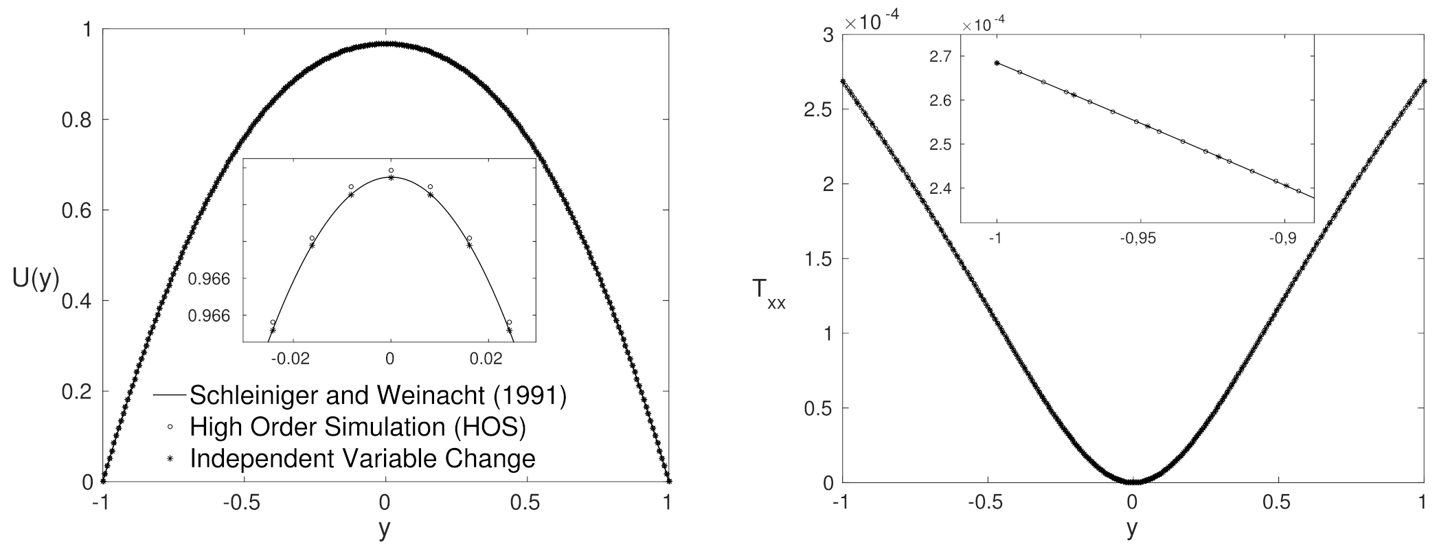
4.1. Agreement Region

In the present section, we present a comparison of the results obtained with the three techniques in a range of parameters, where all are in agreement. In the range of dimensionless parameters adopted in the present section, all of the formulations showed good agreement. The range of parameters adopted here is given by:
  • Reynolds number— 0 < R e < 10,000;
  • Weissenberg number— 0 < W i < 10 ;
  • β parameter— 0.01 < β < 1 ;
  • α G parameter— 0 < α G < 0.5 .
Some results were chosen to show the range mentioned above. These results are presented showing the variation of the streamwise velocity U ( y ) and the three components of the extra-stress tensor T x x , T x y and T y y in the wall-normal direction y.
Figure 1, Figure 2 and Figure 3 show the comparison among the formulations presented for different values of the dimensionless numbers R e , β , and α G in the range of the agreement region.
It is possible to observe very good agreement between the results obtained by different formulations, both for β close to zero (close to polymeric fluid) and for β close to one (close to Newtonian fluid).
For these simulations, different values for the dimensionless parameters of the flow were considered, where all the formulations converge to a solution. It is noteworthy that the formulations have certain limitations for some values for the dimensionless numbers. Out of the agreement region, the results using the first and the second formulation diverges or appears with oscillations on their field. The exploration of these bounds are shown below.

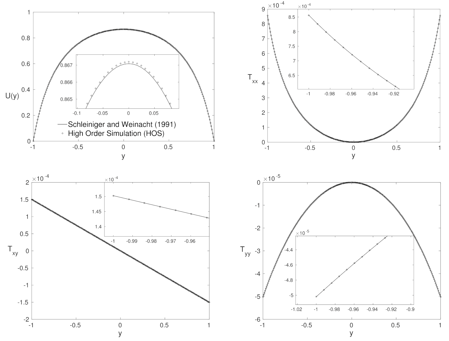
4.2. Purely Polymeric Flows
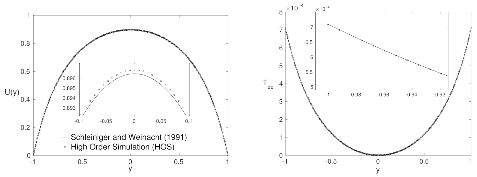
Considering the dimensionless number β = 0 , the flow of a viscoelastic fluid is known as a purely polymeric fluid flow, since there is no Newtonian solvent contribution in the fluid composition.
The independent variable change formulation does not converge for a purely polymeric fluid. Therefore, for flows with β = 0 , the Schleiniger and Weinacht [10] and HOS formulations were used, and their results were compared.
Figure 4, Figure 5 and Figure 6 show the variation of the streamwise velocity U ( y ) and the three components of the extra-stress tensor T x x , T x y and T y y in the wall-normal direction y.
The extra-stress tensor results obtained by the formulations of Schleiniger and Weinacht [10] and HOS, considering the flow for a purely polymeric fluid, showed a good agreement among each other. However, a small difference between the velocity profiles can be observed at the channel center ( u ( y = 0 ) ).

4.3. Low β Number—Close to Purely Polymeric Flows

As mentioned earlier, the formulation using the independent variable change does not work for β = 0 . However, an analysis of the results for this formulation was performed, considering β close to zero. The results obtained by the formulation Schleiniger and Weinacht [10] and by the HOS formulation are compared. The comparisons were carried out for the streamwise velocity U ( y ) and the three components of the extra-stress tensor T x x , T x y and T y y , as can be seen in Figure 7, Figure 8 and Figure 9, for β = 0.1 , 0.05 and 0.01 , respectively.
The results obtained are in agreement, however, as the value of the dimensionless number β decreases, the difference between the formulations increases. This shows precisely the restriction commented above that, for the independent variable change formulation, the lowest value for β has to be β = 0.01 in order to obtain acceptable results with this formulation. It is worth mentioning that, as the solution obtained is analytical for all components, except for the streamwise velocity, the increase in the number of points adopted in the solution did not show an influence for lower values of β simulations.

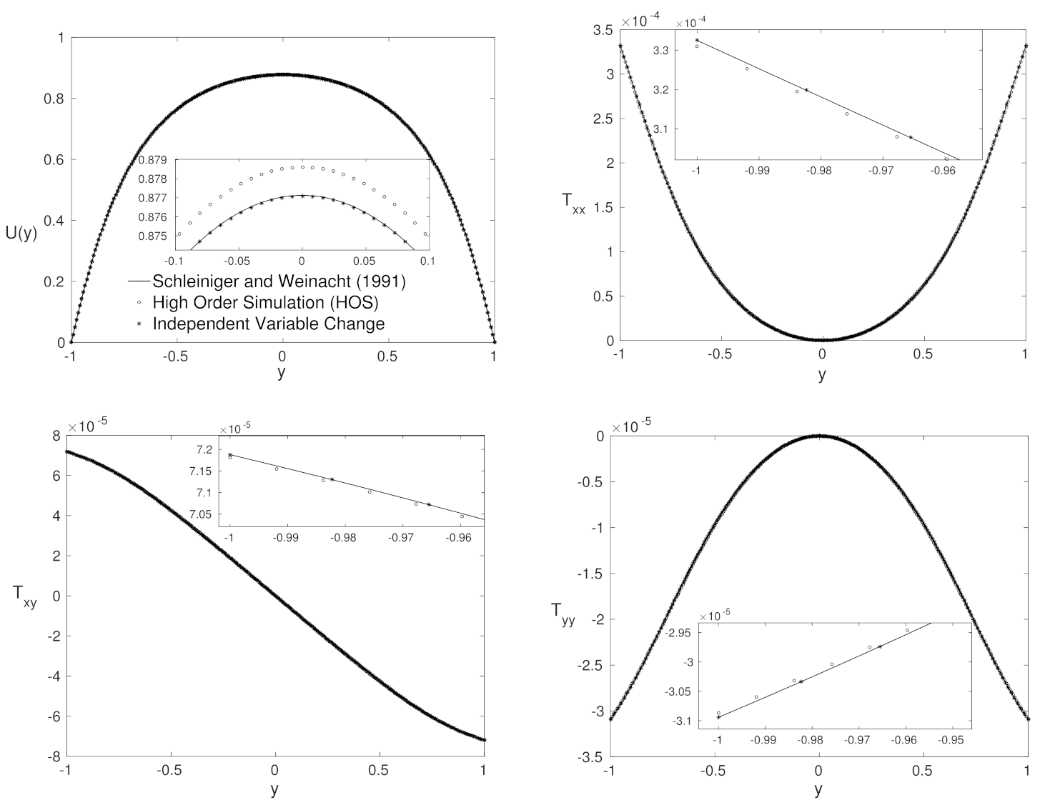
4.4. High Weissenberg Number

The HOS formulation was implemented with the log-conformation technique for flow simulation, considering high values of the Weissenberg number. The SW formulation [10] was not able to converge to the solution when considering R e and W i higher than 8000 and 10, respectively.
However, the formulation based on the independent variable change was able to obtain solutions for any values of R e > 0 , W i > 0 and 0 < α G < 0.5 , with the only restriction to use the dimensionless number β > 0.01 .
Figure 10, Figure 11 and Figure 12 show the variation of the streamwise velocity U ( y ) and the three components of the extra-stress tensor T x x , T x y and T y y in the wall-normal direction y for different dimensionless numbers of R e , β , α G , and with Weissenberg number W i = 150 , 300 , and 500.
One may observe that the results obtained by the different formulations are in agreement. An interesting behavior presented by the HOS formulation can be observed. The results obtained by this formulation, for high Weissenberg numbers, show oscillations for the extra-stress tensor components in the channel center, and as the Weissenberg number increases, the oscillations are more pronounced.
Oscillations usually appear in simulations of flow between parallel plates close to the wall and not in the channel center. However, for high values of the Weissenberg number, a discontinuity is observed in the extra-stress tensor components in the channel center. With the HOS formulation, even using the log-conformation technique to solve the problem of the high Weissenberg number, oscillations were found in the extra-stress tensor components in this region. The use of mesh refinement in the wall-normal direction smooths these oscillations. It is also possible to adopt a stretched mesh, refining only in the region of the channel center to reduce these oscillations and the computational cost.

4.5. Advantages and Disadvantages for Each Formulation

The formulation based on the Schleiniger and Weinacht formulation [10] is advantageous in terms of the velocity cost in obtaining the flow components, because the system of equations is solved in a semi-analytical way. Another advantage of this formulation is the possibility to obtain the flow variables without the contribution of the solvent; that is, flow for the purely polymeric fluid ( β = 0 ). The disadvantage appears in the direction of convergence towards the adequate pressure gradient for the ideal flow. This disadvantage is related to the term inside the square root of Equation (21), it can becomes negative, and the solution is no longer real. This behavior appears for high values of Weissenberg W i , Reynolds number R e , and the mobility parameter α G .
The formulation based on the independent variable change is advantageous for analytically obtaining the main components of the desired flow. Another advantage: there is no restriction for the values of the flow variables, except those already found by Schleiniger and Weinacht [10] (such as α G = 0.5 ). The disadvantage is the computational cost, since it was not possible to obtain an analytical expression for this. It is necessary to interpolate a new distribution for the tensor T x y to find an equally spaced domain of y, then it is numerically integrated to the expression (29), and finally the streamwise velocity component can be obtained. Another disadvantage of this formulation is the limitation of the flow simulation for purely polymeric fluids ( β = 0 ). The limitation arises from the equation for the derivative of velocity (29), where the right-hand side terms are divided by β .
The solution obtained by high-order simulation is advantageous because simplifications are not adopted in the equation system that models the flow, so the problem is solved, considering all of the terms in the equation system. The disadvantage of this formulation is the computational cost, since many CPU hours are necessary to obtain the solution for each case. The adopted code uses domain decomposition parallelization, high-order methods for approximating the spatial derivatives, and a classical fourth-order Runge–Kutta method for the temporal derivative.
The simulations were carried out in a computer Intel Xeon E5-2680v2 2.8 GHz. The wall time required for the Schleiniger and Weinacht [10] and the independent variable change formulations were less than 5 s. The high-order simulations were performed using 16 cores and the wall time was about 20 h.

5. Conclusions

This paper presents three different formulations to obtain the solution of a two-dimensional viscoelastic fluid flow between two parallel plates, modeled by the Giesekus constitutive equation.
The first formulation presented is based on the work by Schleiniger and Weinacht [10]. The second formulation presented is based on the idea of the independent variable change. This change allows the flow components to be obtained analytically, except for the velocity profile, obtained using a high-order numerical integration method. The third formulation presented was called high-order simulation (HOS), i.e., the numerical simulation of the flow modeled by the Navier–Stokes equations and the constitutive equation, using high-order methods to obtain the solution.
The Schleiniger and Weinacht [10] formulation is efficient to obtain the flow components accurately and quickly. However, using many numerical methods for the solution makes convergence difficult for specific parameter values. Each step is verified if the value inside the square root is negative, making the solution complex and no longer real. However, this formulation proved efficient in obtaining the flow components for purely polymeric fluids ( β = 0 ), converging to the solution for almost all values proposed. It did not work for high values of Reynolds R e and Weissenberg W i numbers.
The formulation based on the independent variable change proved to be very efficient, as it solves all of the flow components analytically, but the velocity profile. The flow components are obtained quickly and accurately, for any values of dimensionless numbers of Reynolds R e , Weissenberg W i , α G , and β > 0 . The only limitation of this formulation is when the fluid is composed of purely polymeric fluid flows, or near it β < 0.01 .
The HOS formulation is based on the complete solution of the Navier–Stokes equations and the considered constitutive equation. This formulation has a high computational cost since the simulations take a long time to be solved. However, the numerical methods used proved to obtain good results for the simulations carried out for all of the proposed dimensionless parameters, with a high Weissenberg number, β = 0 , α G , and Reynolds number R e .
It could be observed that the formulations presented proved to be efficient at obtaining the components of the desired flow. The results of the formulations were explored and analyzed, and their respective limitations and efficiencies were commented on. These results could be used to clarify and help researchers with which formulation is most suitable, depending on the fluid and flow parameters adopted.

Author Contributions

Methodology, L.J.d.S.F., M.T.d.A., A.C.B., D.O.d.A.C. and L.F.d.S.; investigation, L.J.d.S.F., M.T.d.A., A.C.B., D.O.d.A.C. and L.F.d.S.; writing—original draft preparation, L.J.d.S.F., M.T.d.A., A.C.B., D.O.d.A.C. and L.F.d.S.; writing—review and editing, L.J.d.S.F., M.T.d.A., A.C.B., D.O.d.A.C. and L.F.d.S. All authors have read and agreed to the published version of the manuscript.

Funding

Research was carried out using the computational resources of the Center for Mathematical Sciences Applied to Industry (CeMEAI), funded by FAPESP grant 2013/07375-0.

Institutional Review Board Statement

Not applicable.

Informed Consent Statement

Not applicable.

Data Availability Statement

Not applicable.

Acknowledgments

L.J.d.S.F., M.T.d.A. and L.F.d.S. acknowledge the Department of Applied Mathematics and Statistics—University of Sao Paulo, Sao Carlos. A.C.B. acknowledges the Department of Mathematics and Computer Science—Sao Paulo State University, Presidente Prudente and D.O.d.A.C. acknowledges the Department of Mechanical Engineering—Federal University of Rio de Janeiro, Rio de Janeiro.

Conflicts of Interest

The authors declare no conflict of interest.

References

  1. Hayat, T.; Khan, M.; Ayub, M. Some simple flows of an Oldroyd-B fluid. Int. J. Eng. Sci. 2001, 39, 135–147. [Google Scholar] [CrossRef]
  2. Hayat, T.; Khan, M.; Ayub, M. Exact solutions of flow problems of an Oldroyd-B fluid. Appl. Math. Comput. 2004, 151, 105–119. [Google Scholar] [CrossRef]
  3. Oliveira, P.J. An exact solution for tube and slit flow of a FENE-P fluid. Acta Mech. 2002, 158, 157–167. [Google Scholar] [CrossRef] [Green Version]
  4. Cruz, D.; Pinho, F.; Oliveira, P. Analytical solutions for fully developed laminar flow of some viscoelastic liquids with a Newtonian solvent contribution. J. Non-Newton. Fluid Mech. 2005, 132, 28–35. [Google Scholar] [CrossRef] [Green Version]
  5. Duarte, A.; Miranda, A.; Oliveira, P. Numerical and analytical modeling of unsteady viscoelastic flows: The start-up and pulsating test case problems. J. Non-Newton. Fluid Mech. 2008, 154, 153–169. [Google Scholar] [CrossRef] [Green Version]
  6. Paulo, G.; Oishi, C.; Tomé, M.; Alves, M.; Pinho, F. Numerical solution of the FENE-CR model in complex flows. J. Non-Newton. Fluid Mech. 2014, 204, 50–61. [Google Scholar] [CrossRef]
  7. Pinho, F.T.; Oliveira, P.J. Axial annular flow of a nonlinear viscoelastic fluid—An analytical solution. J. Non-Newton. Fluid Mech. 2000, 93, 325–337. [Google Scholar] [CrossRef]
  8. Ferrás, L.L.; Nóbrega, J.M.; Pinho, F.T. Analytical solutions for channel flows of Phan-Thien-Tanner and Giesekus fluids under slip. J. Non-Newton. Fluid Mech. 2012, 171–172, 97–105. [Google Scholar] [CrossRef]
  9. Yoo, J.Y.; Choi, H.C. On the steady simple shear flows of the one-mode Giesekus fluid. Rheol. Acta 1989, 28, 13–24. [Google Scholar] [CrossRef]
  10. Schleiniger, G.; Weinacht, R.J. Steady Poiseuille flows for a Giesekus fluid. J. Non-Newton. Fluid Mech. 1991, 40, 79–102. [Google Scholar] [CrossRef]
  11. James, D.F. Boger Fluids. Annu. Rev. Fluid Mech. 2009, 41, 129–142. [Google Scholar] [CrossRef]
  12. Giesekus, H. Elasto-viskose Flüssigkeiten, für die in stationären Schichtströmungen sämtliche Normalspannungskomponenten verschieden gross sind. Rheol. Acta 1962, 2, 50–62. [Google Scholar] [CrossRef]
  13. Raisi, A.; Mirzazadeh, M.; Dehnavi, A.; Rashidi, F. An approximate solution for the Couette–Poiseuille flow of the Giesekus model between parallel plates. Rheol. Acta 2008, 47, 75–80. [Google Scholar] [CrossRef]
  14. Tomé, M.; Araujo, M.; Evans, J.; McKee, S. Numerical solution of the Giesekus model for incompressible free surface flows without solvent viscosity. J. Non-Newton. Fluid Mech. 2019, 263, 104–119. [Google Scholar] [CrossRef]
  15. Giesekus, H. A simple constitutive equation for polymer fluids based on the concept of deformation-dependent tensorial mobility. J. Non-Newton. Fluid Mech. 1982, 11, 69–109. [Google Scholar] [CrossRef]
  16. Giesekus, H. Constitutive equations for polymer fluids based on the concept of configuration-dependent molecular mobility: A generalized mean-configuration model. J. Non-Newton. Fluid Mech. 1985, 17, 349–372. [Google Scholar] [CrossRef]
  17. Fattal, R.; Kupferman, R. Constitutive laws for the matrix-logarithm of the conformation tensor. J. Non-Newton. Fluid Mech. 2004, 123, 281–285. [Google Scholar] [CrossRef]
  18. Fattal, R.; Kupferman, R. Time-dependent simulation of viscoelastic flows at high Weissenberg number using the log-conformation representation. J. Non-Newton. Fluid Mech. 2005, 126, 23–37. [Google Scholar] [CrossRef]
  19. Souza, L.F.; Mendonça, M.T.; Medeiros, M.A.F. The advantages of using high-order finite differences schemes in laminar-turbulent transition studies. Int. J. Numer. Methods Fluids 2005, 48, 565–592. [Google Scholar] [CrossRef]
  20. Ferziger, J.H.; Peric, M. Computational Methods for Fluid Dynamics; Springer: Berlin/Heidelberg, Germany; New York, NY, USA, 1997. [Google Scholar]
  21. Stüben, K.; Trottenberg, U. Nonlinear Multigrid Methods, The Full Approximation Scheme; Springer: Koln-Porz, Germany, 1981; Chapter 5; pp. 58–71. [Google Scholar]
  22. Souza, L.F. Instabilidade Centrífuga e Transição Para Turbulência em Escoamentos Laminares Sobre Superfícies Côncavas. Ph.D. Thesis, Instituto Tecnológico de Aeronáutica, Sao Jose dos Campos, Brazil, 2003. [Google Scholar]
  23. Lele, S. Compact Finite Difference Schemes with Spectral-Like Resolution. J. Comput. Phys. 1992, 103, 16–42. [Google Scholar] [CrossRef]
Figure 1. Streamwise velocity U ( y ) and the components of the extra-stress tensor T x x , T x y and T y y variation in the wall-normal direction y. Dimensionless numbers: R e = 2000 , β = 0.25 , α G = 0.1 and W i = 2 .
Applsci 11 10115 g001
Figure 2. Same as in Figure 1 for dimensionless numbers: R e = 5000 , β = 0.5 , α G = 0.2 and W i = 2 .
Applsci 11 10115 g002aApplsci 11 10115 g002b
Figure 3. Same as in Figure 1 for dimensionless numbers: R e = 8000 , β = 0.75 , α G = 0.2 and W i = 2 .
Applsci 11 10115 g003
Figure 4. Same as in Figure 1 for dimensionless numbers: R e = 2000 , β = 0 , α G = 0.3 and W i = 2 .
Applsci 11 10115 g004
Figure 5. Same as in Figure 1 for dimensionless numbers: R e = 5000 , β = 0 , α G = 0.2 and W i = 2 .
Applsci 11 10115 g005
Figure 6. Same as in Figure 1 for dimensionless numbers: R e = 8000 , β = 0 , α G = 0.1 and W i = 2 .
Applsci 11 10115 g006aApplsci 11 10115 g006b
Figure 7. Same as in Figure 1 for dimensionless numbers: R e = 5000 , β = 0.1 , α G = 0.3 and W i = 2 .
Applsci 11 10115 g007aApplsci 11 10115 g007b
Figure 8. Same as in Figure 1 for dimensionless numbers: R e = 8000 , β = 0.05 , α G = 0.3 and W i = 2 .
Applsci 11 10115 g008
Figure 9. Same as in Figure 1 for dimensionless numbers: R e = 2000 , β = 0.01 , α G = 0.3 and W i = 2 .
Applsci 11 10115 g009
Figure 10. Same as in Figure 1 for dimensionless numbers: R e = 2000 , β = 0.25 , α G = 0.1 and W i = 150 .
Applsci 11 10115 g010
Figure 11. Same as in Figure 1 for dimensionless numbers: R e = 8000 , β = 0.5 , α G = 0.3 and W i = 300 .
Applsci 11 10115 g011aApplsci 11 10115 g011b
Figure 12. Same as in Figure 1 for dimensionless numbers: R e = 5000 , β = 0.75 , α G = 0.2 and W i = 500 .
Applsci 11 10115 g012
Publisher’s Note: MDPI stays neutral with regard to jurisdictional claims in published maps and institutional affiliations.

