MiA-CODER: A Multi-Intelligent Agent-Enabled Reinforcement Learning for Accurate Coverage Hole Detection and Recovery in Unequal Cluster-Tree-Based QoSensing WSN

Abstract

Coverage is an important factor for the effective transmission of data in the wireless sensor networks. Normally, the formation of coverage holes in the network deprives its performance and reduces the lifetime of the network. In this paper, a multi-intelligent agent enabled reinforcement learning-based coverage hole detection and recovery (MiA-CODER) is proposed in order to overcome the existing challenges related to coverage of the network. Initially, the formation of coverage holes is prevented by optimizing the energy consumption in the network. This is performed by constructing the unequal Sierpinski cluster-tree topology (USCT) and the cluster head is selected by implementing multi-objective black widow optimization (MoBWo) to facilitate the effective transmission of data. Further, the energy consumption of the nodes is minimized by performing dynamic sleep scheduling in which Tsallis entropy enabled Bayesian probability (TE2BP) is implemented to switch the nodes between active and sleep mode. Then, the coverage hole detection and repair are carried out in which the detection of coverage holes if any, both inside the cluster and between the clusters, is completed by using the virtual sector-based hole detection (ViSHD) protocol. Once the detection is over, the BS starts the hole repair process by using a multi-agent SARSA algorithm which selects the optimal mobile node and replaces it to cover the hole. By doing so, the coverage of the network is enhanced and better QoSensing is achieved. The proposed approach is simulated in NS 3.26 and evaluated in terms of coverage rate, number of dead nodes, average energy consumption and throughput.

1. Introduction

The wireless sensor network (WSN) has wide applications in many fields like healthcare, monitoring applications and disaster recovery applications. In any application, the prime objective of the sensor network is to provide the proper sensing results by improving the quality of sensing (QoSensing). The QoSensing is directly proportional to the coverage rate, i.e., when the whole network is covered then the QoSensing is better in the network. One of the significant ways to achieve a better coverage rate is to deploy the sensor nodes in the optimal position where multiple objectives are to be satisfied for better coverage [1]. The target coverage sensors were found to overcome the coverage issues in which the sensors having poor coverage were eliminated and the sensors having contributing maximum coverage were considered [2]. The holes in the coverage area are caused due to the non-line of sight issues which result in the degradation of QoSensing in the WSN. In order to overcome this problem, the distributed self-healing approach was implemented which was found to improve the coverage [3]. The reposition of nodes and adjustment of the sensing range resulted in recovery from coverage holes which eventually increased the coverage resulting in improved QoSensing in the network [4]. The placement of relay nodes in the network increased the coverage but the location of these extra nodes introduced placement issues and also increased the deployment cost [5]. The QoSensing was also affected by the increased consumption of energy by the sensing nodes. The detection of boundary nodes is an important factor to optimize the energy consumption which includes the detection of event boundary nodes and coverage hole boundary nodes [6]. The energy consumption of the sensor nodes was reduced by implementing the process of clustering in which the sensor nodes were clustered, and the cluster head was elected. In order to reduce the energy consumption further the path selection was executed based on optimization [7]. The scheduling of nodes between the active and sleep mode contributed to improved energy efficiency which further increased the lifetime of the network. This method not only solved coverage issues but also improved throughput in the network [8]. The improvement in the coverage was introduced by selecting the optimal coverage area with flexibility in field of view, but inefficient optimization resulted in increased redundancy [9]. The technique optimization was implemented for the efficient placement of sensor nodes in order to improve the coverage in the network [10]. The technology of unmanned aerial vehicles was leveraged in wireless sensor networks in which the sensor nodes offloaded the data to the UAVs which improved the network coverage and reduced the consumption of energy [11]. The combination of coverage optimization and energy regulation processes increased the QoSensing of the transmission and extended the lifetime of the sensor nodes [12]. The implementation of the mobile sink comparatively increased the network coverage, and further, the usage of the long-range wireless interface improved the QoSensing of the network [13]. The deployment of sensors in zone-based regions based on the detection probabilities solved the coverage problems but increased the deployment cost limiting the adoption of this method in real-life scenarios [14]. The positioning of the sensor nodes was performed in three dimensions which was said to improve the accuracy in positioning the nodes and thereby determining the coverage area, but the coverage problem was not addressed efficiently [15].

1.1. Motivation and Objectives

This research work aims to enhance QoSensing in WSNs. For that purpose, this work is interested in achieving a better coverage rate by repairing coverage holes and improving the energy efficiency in the network. The deployment of both static and mobile nodes is executed to accomplish the goal. The objectives of this research paper are as follows:

• To partition the network in a better way such that the hotspot problem can be mitigated.
• To find the optimal header nodes to enhance the data transmission.
• To turn off the radio of needy nodes to prevent the node death, i.e., to prevent the holes.

1.2. Research Contributions

We mainly focus on enhancement of the coverage and optimization of energy consumption in the network to achieve better QoSensing. The following are the major contributions of this work:

• A robust network topology is built by implementing the unequal Sierpinski cluster-tree topology (USCT) in order to improve the energy efficiency in the transmission of data.
• The optimal cluster head selection is performed by multi-objective black widow optimization (MoBWo) to increase the efficiency of data transmission.
• The dynamic sleep scheduling is carried out to further reduce the energy consumption by the node which is carried out by the Tsallis entropy enabled Bayesian probability (TE2BP) algorithm.
• The coverage hole is detected both inside the cluster and between the clusters by implementing the virtual sector-based hole detection (ViSHD) protocol.
• A novel multi-agent SARSA (MA-SARSA) algorithm is presented to learn the environment and repair the holes to achieve better QoSensing.

1.3. Paper Organization

The organization of this research work is as follows: section II presents the detailed explanation of related works proposed in coverage hole detection and efficient energy consumption for effective data transmission. In section III, the major problem statements are discussed and the research gaps in enhancement of coverage are analyzed. In section IV, the methodology proposed in this research work is described in an elaborate manner. Section V presents the experimentation of the proposed work and validation of the performance through several metrics. In section VI, the conclusion and future work of this research work are presented briefly.

2. Related Work

Authors in [16] mainly concentrate on coverage hole detection through participated nodes and coverage hole recovery by maximizing the sensing range of those nodes. For that, this paper presents a heuristic hole healing (H3) algorithm. The H3 algorithm first performs hole detection based on the radius of the nodes participating in the network. Then, the optimal node is selected to repair the hole through the H3 algorithm. The optimal node is selected based on overlapping degree and residual energy level. The H3 algorithm uses a fuzzy inference system (FIS) to select an optimal node. The optimal moving distance and sensing are also determined to heal the coverage hole. Sensing range maximization is a traditional approach to heal the coverage problem. However, this method increases the energy consumption and complexity for the optimal node that is selected to heal the hole. The overall network is considered to be mobile, but the optimal node detection does not consider any mobility metrics. Thus, there will be frequent coverage hole occurrences whenever the healing node moves to another position. In [17], the authors focus on coverage hole detection and enhancement in WSNs. For that, this work presents a hybrid hole healing algorithm (3HA). This work determines the optimal position to improve the coverage rate. Then, new additional nodes are deployed in the determined position in order to improve the coverage ratio. The 3HA algorithm is performed in a distributed manner. At first, the coverage hole is detected by constructing a Voronoi diagram for the network. Then, the Voronoi list is reduced to formulate linear programming and a probabilistic sensing model. Nevertheless, adding additional nodes increases the deployment cost and the holes are not fully recovered, and the construction of a Voronoi diagram is a complex process and consumes a large amount of time.

In [18], the authors dynamically analyze the network and determine the coverage holes. Firstly, the network topology is analyzed based on a simple subnet. Upon the subnet, the boundary nodes are determined, and the area of polygon is computed. Three categories of subnets such as (i) with simple subnet, (ii) without isolated nodes and (iii) with multiple subnets are considered for a better analysis. As the recovery mechanism, the inactive nodes are activated. For that, the network is initialized with active and inactive nodes. When the coverage hole occurs, then the inactive node is activated to repair the coverage hole. However, the coverage hole recovery process is not efficient since it simply activates the random nodes without considering the network environment and there is a high possibility to form new holes due to the high energy consumption. In [19], the authors propose a cluster-based routing approach to achieve better energy efficiency. For that, a multi-objective fractional particle lion (MOFPL) algorithm is proposed. The MOFPL algorithm combines the particle swarm optimization and lion optimization algorithm with the concept of fractional theory. Initially, the network is clustered, and the cluster head (CH) is assigned in each cluster. Then, the optimal CH is selected to enable routing based on multiple objectives such as energy, distance, delay, density and traffic rate. Through the optimal CH, the data are transmitted to the BS. However, PSO and lion optimization are combined with fractional theory to improve the convergence rate. This results in large time consumption. Initially, CHs are randomly selected which increases energy consumption.

Authors in [20] mainly focus on optimal CH selection to improve the energy efficiency. To enable optimal CH selection, a hybrid optimization algorithm is presented. The hybrid algorithm is built with the crow search algorithm and dolphin echolocation algorithm. The objective is formulated to enhance data transmission and also to enhance energy efficiency. The proposed hybrid algorithm considers multiple objective functions such as link lifetime, intra-cluster distance, mobility, delay, energy and inter-cluster distance. However, consideration of inter-cluster distance in the CH selection is inefficient since it can be computed only after all CHs are selected, and the formation of equal size clusters leads to a hotspot problem. In [21], the authors propose a duty cycling method for improving delay and energy efficiency in WSNs. To achieve this objective, this paper presents a dynamic duty cycle (DDC) scheme in the WSN. In this paper, the interrelation between duty cycling and delay is analyzed deeply to frame optimal adaptive duty cycling. Here, the large duty cycle, i.e., the awake period, is assigned to the nodes which are positioned far away from the sink node. These nodes are known as the nodes in non-hotspot areas. The sleep slot is assigned for the nodes in the hotspot area on the basis of residual energy level. However, the hotspot problem is not fully mitigated.

In [22], the authors improve the energy efficiency through multiple procedures. Chiefly, a ring-partitioning-based sleep scheduling protocol is proposed to achieve better energy efficiency. Initially, the network is divided into multiple clusters by a weighted Voronoi diagram. Then, a two-fold data aggregation scheme is enabled to minimize the energy consumption further. Intra-cluster routing is enabled by hybrid chicken swarm optimization while an inter-cluster routing algorithm is presented with position-based routing tree construction. Nevertheless, the weighted Voronoi diagram-based clustering process increases complexity, and the RP-MAC protocol assigns sleep slots for the nodes in a random manner which degrades the performance of the network. Authors in [23] focus on QoSensing enhancement in a WSN for water monitoring applications. Here, the QoSensing is enhanced by improving the coverage ratio of the network. The aim of this work is to detect the water contamination using sensor nodes. For that, the budget constrained optimal position of the sensor nodes is determined. The budget is minimized by positioning the sensor nodes in an optimal position. To find the optimal position, this work uses a genetic algorithm (GA) which selects the optimal position for the nodes. At last, the nodes are deployed in the optimal positions in order to detect the water contamination. In general, coverage holes are formed with the increase in data transmission. This work only considers the coverage holes at the initial phase; therefore, QoSensing is better in the initial stage and degrades over the time period. Hence, this work is unable to maintain better QoSensing in the network. Although nodes are placed in an optimal position, when the energy level of a node decreases then the node must be replaced. This leads to coverage holes which degrade QoSensing.

Authors in [24] insist that the importance of reliability in the WSN and the connectivity between the nodes in the network is addressed. This is achieved by implementing a network topology-based approach in which the nodes in the network are constructed as a spanning tree which greatly reduces the link failure problem in the network. The transmission of data is facilitated through the nodes which are arranged in a tree-shaped topology. However, the energy consumption in the network is not addressed which will lead to the problem of coverage holes in the network, thereby affecting the QoS of the network. According to the authors in [25], the placement of the nodes in the network is carried out in an optimal manner. The optimization of node placement is performed in a regional manner based on coverage and energy consumption. Hence, the necessary nodes to be moved are reduced which further reduces the overhead in the network. This approach leads to experimentation, and the results show that it has better performance since it considers both coverage and energy consumption in the network. However, the detection and reduction of coverage holes in the network are not considered which also affects the effective transmission of data in the network.

Authors in [26] focus on the deployment of wireless sensor networks using optimization techniques. Initially, the applications of WSN in various fields are mentioned and the necessity of the proper deployment of sensors in the network is addressed. The geo-spatial information system-based optimization is implemented in order to deploy the IoT sensors in an optimal manner. Two algorithms, namely, particle swarm optimization (PSO) and bees algorithm (BA) were experimented with, and the results show that the former algorithm has better convergence and the latter one has better fitness value computation. In spite of the deployment of sensor nodes, the coverage hole problems arise and a proper method to enhance the coverage in the network is not addressed. According to the authors in [27], a sensor deployment strategy is implemented to facilitate the effective data transmission in smart cities. The deployment of sensors is carried out in a careful manner in order to provide better coverage and a low economical budget. Initially, the Voronoi diagram is constructed and the Delaunay triangle is constructed between the randomly deployed IoT sensors. The triangle’s center point is computed in order to deploy the remaining sensors in high coverage points. The clustering of nodes is executed based on k-means clustering and the sink nodes are deployed in the center of the cluster for better coverage.

3. Major Problem Statement

This section briefly explains the research barriers in enhancing the coverage of the network by the efficient consumption of energy to achieve better QoSensing. The existing works do not provide an overall solution for achieving better QoSensing in which either coverage enhancement or energy consumption is optimized; however, both these factors must be focused on to accomplish the objective. The overall problem in this research topic is mentioned below.

Authors in [28] indicate how the quality of sensing (QoSensing) decides the overall performance of the network. In any application, the WSN aims to achieve better QoSensing. In general, the QoSensing is measured in terms of coverage ratio. To enhance the coverage ratio, existing works have focused on two methods: (i) optimal sensor deployment (initial stage) and (ii) coverage enhancement (hole detection and recovery (after deployment)). The first method requires a high cost to find the optimal position for all nodes and is not suitable for large-scale networks. Hence, the coverage enhancement procedure has been followed by many works. However, these methods fail to detect the hole accurately and to recover the hole by using a minimal number of nodes due to poor algorithm design, limited metrics consideration and so on. Besides, the formations of hotspots due to energy consumption of the nodes are the major factors for coverage holes. Thus, improving energy efficiency also helps in enhancing QoSensing by preventing the coverage holes. However, energy efficiency enhancement to improve QoSensing is lightly focused on by the authors. The prevention of coverage holes will reduce the overhead of the coverage hole recovery phase.

Authors in [29] aim to improve the coverage ratio in the WSN. The overall sensor network is considered as equal size grids. Then, the grids with the minimum coverage ratio are considered as the candidate grids. Next, the grids which have a coverage ratio lower than the threshold value are considered for the coverage enhancement process. In those grids, the mobile nodes are optimally positioned in order to ensure proper coverage. To find the optimal position for mobile nodes, this work uses the particle swarm optimization (PSO) algorithm. The PSO algorithm considers moving distance as the metric in order to minimize energy consumption. The major problems encountered in this approach are:

• The PSO algorithm finds the optimal position for the mobile nodes but is not able to find which nodes to move. Considering random mobile nodes in the PSO algorithm increases energy consumption further, i.e., if the selected mobile node is far away from the hole, then the node must travel for a long distance.
• Equal grid construction leads to coverage holes due to high energy consumption in particular nodes.
• The PSO algorithm has convergence issues which lead to mobile movement non-optimally.

According to the authors in [30], the coverage hole detection problem is resolved by using different concepts and theorems. Mainly, this work utilizes the Rips complex concept to detect the coverage hole. To simplify the Rips complex, first the Turan’s theorem is combined with the clustering coefficient. This process removes the redundant nodes by putting them in sleep mode. By removing the redundant nodes, the network is simplified. Next, the concept of a complete graph is utilized to remove the redundant edges. At last, the Rips complex is applied on the simplified network in order to detect the hole detection. The problems faced by this work are as follows:

• To simplify the network, this work puts the nodes with large clustering coefficients into sleep mode. Although it simplifies the network, it affects the connectivity among other nodes. It also results in large coverage holes. In addition, turning off the node with the higher clustering coefficient also leads to a higher number of holes in the network.
• In general, the Rips complex concept is complex and not suitable for the resource-constrained sensor networks.
• This work only identifies the hole and is unable to heal the hole which plays a vital role in coverage enhancement. In addition, the efficacy of the coverage hole detection can be measured only after the recovery process. Thus, this work is inefficient to improve the coverage of the network.

Authors in [31] aim to improve energy efficiency in the network through optimal cluster formation and sleep scheduling. Firstly, the network is segregated into multiple clusters by base station (BS). For optimal cluster head (CH) selection, a probability value which is composed of energy and traffic rate metrics is formulated. In each cluster, the nodes which are located nearby are paired. The nodes which have no neighbor nodes are isolated and the nodes directly communicate with the cluster head (CH). The time division multiple access (TDMA) scheduling technique is revised to support data gathering. The sleep scheduling is performed among the paired nodes. The problems encountered in this research work are:

• Here the sleep scheduling is rotated among only paired nodes, i.e., isolated nodes have no opportunity to sleep. This scheduling increases energy consumption of the isolated nodes which further results in the early death of nodes.
• Among the paired nodes, the sleep decision is made in a distributed manner which increases control packet overhead and energy consumption in the network.
• CH is selected with the limited metrics (energy level and traffic rate) and the same CHs are used to route the packets. This way of routing increases the packet loss.

Authors in [32] propose a routing algorithm to improve the energy efficiency of the sensor network. For that, a dynamic multi-hop routing protocol is presented in this work. Initially, the network is split into multiple clusters by using a k-means algorithm. In each cluster, optimal CH is selected by using an artificial bee colony (ABC) algorithm. The ABC algorithm considers multiple objectives such as energy level, traffic rate, etc., for optimal CH selection. Then, inter-cluster routing is enabled by using a multi-hop routing approach. The routing approach constructs the objective to minimize hop count and selects a route with a minimum hop count. The following are the issues faced in this research work:

• In the k-means algorithm, initialization of k is relatively difficult and also initialization of centroid nodes also affects the overall clustering process.
• The ABC algorithm has a slow convergence rate and high computational complexity. It selects non-optimal CHs even with large time consumption.

Table 1. Research gaps in previous works.

Method/Technique	Concept	Drawback
CHPS [29]	Positioning of mobile nodes using PSO	High energy consumption/Convergence issues
SRC [30]	Removes the redundant nodes and use Rips complex to detect coverage holes	Affects connectivity/Highly complex for resource constraint devices
SA-CRP [31]	Implements TDMA to schedule the nodes into sleep and active mode	Control packet overhead/Increased packet loss
MOMHR [32]	Cluster formation and routing to minimize hop counts	High complexity/Large time consumption

illustrates the research gaps encountered in previous works from which the proposed work is presented as a solution to these problems by enhancing the coverage and energy efficiency to achieve better QoSensing.

4. Proposed Work

To overhaul all of the above research problems and to achieve better QoSensing, we present a novel multi-intelligent agent-based reinforcement learning for accurate coverage hole detection and recovery (MiA-CODER) mechanism in unequal cluster-tree-based WSN to achieve better QoSensing (Figure 1). The proposed network is constructed with static sensor nodes, mobile sensor nodes and a base station (BS) positioned at the center of the network. The overall explanation of the proposed system model is illustrated in the following sections.

4.1. Unequal Cluster-Tree Topology Construction

Table 2. Notations table.

Notations	Description	Notations	Description
V	Denotes the sensors deployed	df	Energy required for CH to perform aggregation
E	Connectivity of the nodes	$\left(CH-intra\left(en\right)\right)$	Energy required for CH in intra-cluster routing
p, q	Two sensor nodes in the network	$\left(CH-R_x-intra\left(en\right)\right)$	Energy required for CH in reception of signals inside the cluster
TR	Range of transmission	$\left(CH-df-intra\left(en\right)\right)$	Energy required for CH in aggregation of received signals from CM
c	Cluster comprising of p number of nodes	$\left(CH-inter\left(en\right)\right)$	Energy required for CH in inter-cluster routing
cp	Cluster center	$\left(CH-T_x-intra\left(en\right)\right)$	Energy required for CH in transmission of signals between the clusters
$X_{N,i}$	Total number of nodes in the network for CH election	$\left(CH-CS-inter\left(en\right)\right)$	Energy required for CH in sensing of signals
RE	Remaining energy	$\mathrm{idle} \left(en\right)$	Energy required in idle state
𝑇𝑥(𝑒𝑛)	Energy required for transmission	a, b	Distance between two nodes in the cluster
R𝑥(𝑒𝑛)	Energy required for reception	C	Capacity of the node referred to in terms of buffer size
k	Length of message bits	CR	Current ratio
${\epsilon }_{ap}, {\epsilon }_{sp}$	Power consumption of amplifier in two-hop	PM	Profit margins
$e{n}_{elec}$	Signal processing energy	P(A)	Probability of node being in active mode
CS (en)	Sensing cost	P(S)	Probability of node being in sleep mode
CM	Cluster members	R	Sum of evidence of the values of residual energy
$Ty$	Tsallis entropy index	$E_{bn}$	Energy boundary nodes

details the list of notations that are used in the paper.

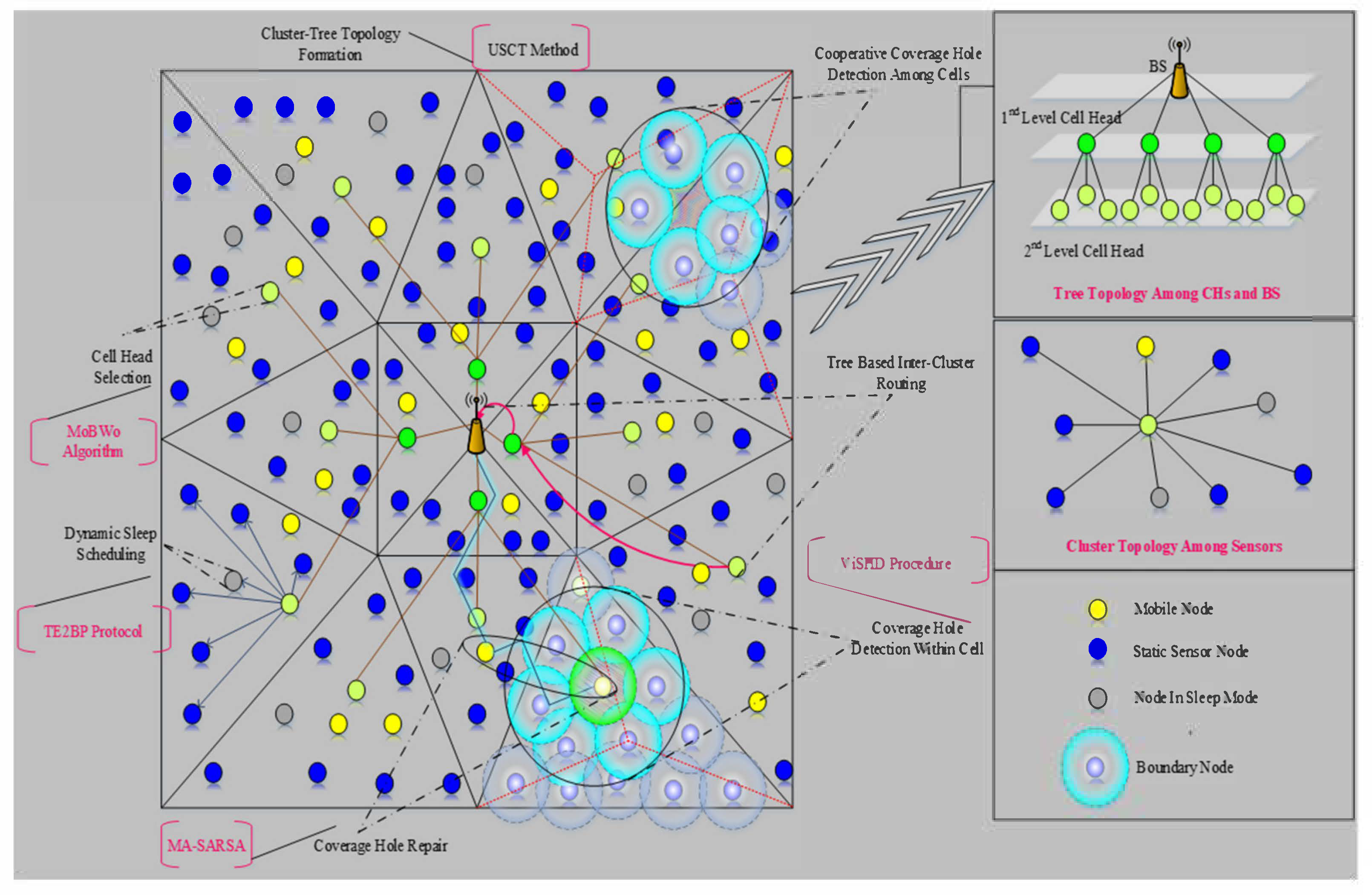
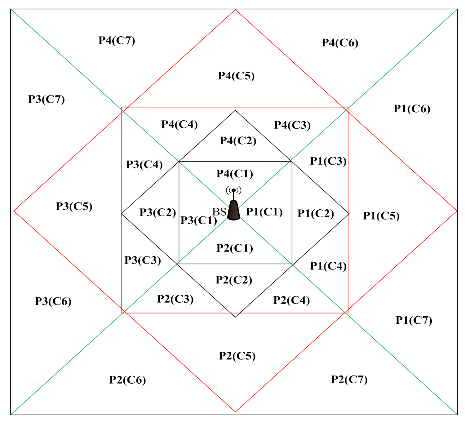
In this phase, we aim to construct a new topology that supports energy efficiency with effectual data transmission. We propose a novel clustering method by considering the triangle-based partitioning of the unequal Sierpinski cluster-tree topology (USCT) construction method in the IoT environment based on the formation of triangle partitions $P=\left\{P1, P2, P3, P4\right\}$ to avoid the coverage hole as shown in Figure 2. The proposed USCT method constructs unequal cells by following the procedure of the Sierpinski triangle. Initially, the network is constructed as a graph N = $V,E$ in which V denotes the sensors deployed and E = $\left\{\left(p,q\right)/dist\left(p,q\right)\le TR\right\}$ represents the connectivity of the nodes. In which p, q are any two sensor nodes in the network, TR denotes the range of transmission. c = {$p\subset V$} is a cluster comprising of a subset of vertices $p$ (nodes) whose center is denoted as $ct$. The cluster tree topology is utilized in which all the nodes are linked with each other which reduces the data loss problem in the network. The network is divided into four triangles and the remaining triangles are formed by repeating the above process to cover the entire area. By doing so, the unequal clusters are formed in which the size of the triangles nearer to the base station is larger than the size of the triangles that are situated away from the base station. Algorithm 1 describes the steps involved in the formation clusters in the network.

Algorithm 1 Cluster Formation

i ← number of iterations;

Rectangular zone diagonals are drawn;  Partition formation $\mathit{P}=\left\{\mathit{P}\mathbf{1}, \mathit{P}\mathbf{2}, \mathit{P}\mathbf{3}, \mathit{P}\mathbf{4}\right\}$;  For each partition do  The clusters are formed, i.e., $\mathit{P}\left(\mathit{C}\mathit{n}\right)$;  Where n = 1, 2, 3…, m;

While i $\ge$ 1 do

For each cluster do

The nearest cluster to BS is considered;

Midpoints of the sides are connected;

i = i−1;

End

End

Once the clusters are formed, the cluster head selection takes place by implementing multi-objective black widow optimization (MoBWo). The main purpose of choosing this algorithm is an early convergence, and it obtains the optimized fitness values as compared to other algorithms such as PSO, GA and other traditional algorithms. In order to choose the proper CH for data collection and aggregation, various sets of parameters are biologically optimized in MoBWo that are follows,

• Spider Size = 40
• Total Number of Generations = 100
• Reproduction Rate = 0.6
• Cannibalism Rate = 0.44
• Mutation Rate = 0.4

The MoBWo is processed by random initialization of the black widow population. Two kinds of spiders’ behavior are inherited in the CH selection, i.e., male black widow and female black widow. The initialization of black widow spiders is given in below,

$$X_{N,i}=\left[\begin{array}{ccc}{x}_{1,1}& x_{1,2}& x_{1,i}\\ x_{2,1}& x_{2,2}& x_{2,i}\\ x_{N,1}& x_{N,1}& x_{N,i}\end{array}\right]$$

(1)

where $X_{N,i}$ are the initial values of the population. In this paper, $X_{N,i}$ is represented as the total number of nodes in the network for CH selection.

The CH is selected based on multiple objectives like energy objective, distance objective and capacity objective. For optimum CH selection, these objectives must be defined as follows:

• Energy objective: residual energy must be higher to elect that node for CH, since minimum energy causes packet retransmission or packet losses issues.
• Distance objective: distance must be lower than the BS to choose it as the CH. Longer distance causes the huge end-to-end delay.
• Capacity objective: a node must consist of lower capacity because a lower capacity node can carry the huge amount of packets from the CM.

Based on the above objectives, the best set of nodes is selected as CH in the number of triangles. Each objective metric can be calculated by the following.

The remaining energy of the sensor node is expressed as,

$$RE=\sum \{T_x\left(en\right) + R_x\left(en\right) + idle\left(en\right) + sleep\left(en\right)\}-IE$$

(2)

$$T_x\left(en\right) = T_x\left(e{n}_{elec}\right) + T_x\left(e{n}_{amp}\right) = \left\{\begin{array}{c}ke{n}_{elec}+k{\epsilon }_{sp}dis{t}^2, \left(CM to CH\right)\\ ke{n}_{elec}+k{\epsilon }_{ap}dis{t}^4, \left(CH to BS\right)\end{array}\right.$$

(3)

In which,$T_x\left(en\right)$ denotes energy required for transmission,${\epsilon }_{sp} and {\epsilon }_{ap}$ denotes power consumption of amplifier in free space and multi-path fading channel models and $e{n}_{elec}$ denotes the signal processing energy, IE represents initial energy, $e{n}_{amp}$ denotes energy required for amplification and k represents length of message bits.

$$R_x\left(en\right) = R_x\left(e{n}_{elec}\right)$$

(4)

In order to compute the energy consumption of the CH, both the energy consumption during inter-cluster and intra-cluster routing are to be calculated which are expressed as the following equations. Equation (5) represents the energy required for CH in intra-cluster routing $\left(CH-intra\left(en\right)\right)$ which is equal to the sum of the energy required for reception of signals inside the cluster $\left(CH-R_x-intra\left(en\right)\right)$ and the energy required for aggregation of received signals $\left(CH-df-intra\left(en\right)\right)$. In Equation (6), the energy consumption of CH in inter-cluster routing $\left(CH-inter\left(en\right)\right)$ is computed which equals to the sum of energy required for the transmission of signals between the clusters $\left(CH-T_x-intra\left(en\right)\right)$ and the energy required for the sensing of signals $\left(CH-CS-inter\left(en\right)\right)$, where $\gamma$ denotes the compression ratio and $CS\left(en\right)$ denotes the sensing cost. The total energy consumption of the wireless sensor network is found from the remaining energy, which can be calculated from Equations (8)–(10).

$$\begin{gathered} CH-intra\left(en\right)=CH-R_x-intra\left(en\right)+CH-df-intra\left(en\right) \\ \begin{array}{c}=ke{n}_{elec}+\left(n+1\right)kdf\left(en\right)\\ =k(ne{n}_{elec}+\left(n+1\right)df\left(en\right)\end{array} \end{gathered}$$

(5)

$$\begin{gathered} CH-inter\left(en\right)=CH-T_x-intra\left(en\right)+CH-CS-inter\left(en\right) \\ \begin{array}{c} =\left(n+1\right)\gamma \left(ke{n}_{elec}+k{\epsilon }_{ap}dis{t}^4\right)+\left(n+1\right)kCS\left(en\right)\\ =\left(n+1\right)k\left(\gamma (e{n}_{elec}+{\epsilon }_{ap}dis{t}^4\right)+CS\left(en\right)\end{array} \end{gathered}$$

(6)

$$\begin{gathered} CH\left(en\right)=CH-intra\left(en\right)+CH-inter\left(en\right) \\ =k((ne{n}_{elec}+\left(n+1\right)df\left(en\right)+\left(n+1\right)\left(\gamma (e{n}_{elec}+{\epsilon }_{ap}dis{t}^4\right)+CS\left(en\right) \end{gathered}$$

(7)

$$CM-CH\left(en\right)={{\displaystyle \sum }}_{j=1}^{n}CM-CH\left(en\right)={{\displaystyle \sum }}_{j=1}^{n}k\left(e{n}_{elec}+{\epsilon }_{sp}dis{t}^2\right)$$

(8)

$$total\left(en\right)={{\displaystyle \sum }}_{j=1}^{n}CH\left(en\right)+CM-CH\left(en\right)$$

(9)

$$=k{\displaystyle \sum }_{j=1}^n\left(\left(ne{n}_{elec}+\left(n+1\right)df\left(en\right)+\left(n+1\right)\left(\gamma (e{n}_{elec}+{\epsilon }_{ap}dis{t}^4\right)+CS\left(en\right)\right)+{\displaystyle \sum }_{j=1}^{n}k\left(e{n}_{elec}+{\epsilon }_{sp}dis{t}^2\right)\right)$$

(10)

$R_x\left(en\right)$ denotes energy required for reception, $idle\left(en\right)$ denotes energy required in idle state and $sleep\left(en\right)$ denotes energy required in sleep state. The remaining energy for all the nodes is calculated to select the optimal cluster head. The distance between two nodes a and b in the cluster is formulated as,

$$Dist\left(a,b\right)=\sqrt{{\left(a_y+b_y\right)}^2+{\left(a_z+b_z\right)}^2}$$

(11)

In which y and z denote the location coordinates of the sensors, respectively. The capacity of the node is referred in terms of buffer size which can be represented as,

$$C=\frac{Initia{l}_{BS}}{initial{ }_{BS}-current{ }_{BS}}$$

(12)

The MoBWo computes the fitness value for each node based on the objective and selects the optimal cluster head. In the procreation mode two nodes are selected as parents and two nodes are selected as children in which the child nodes are expressed as,

$$\left\{\begin{array}{c}{q}_1=\gamma \times p_1+\left(1-\gamma \right)\times p_2\\ q_2=\gamma \times p_2+\left(1-\gamma \right)\times p_1\end{array}\right.$$

(13)

Once the procreation mode selects the nodes, the cannibalism mode is carried out in which only the fittest nodes are selected. Based on the population of the procreation mode, the mutation is carried out and finally the optimal CH is selected. The nodes in each cell form clusters with the CH while the CHs form tree with BS. Data transmission takes place through the CHs selected optimally by the MoBWo algorithm. This phase minimizes energy consumption and increases data transmission efficiency. Algorithm 2 explains the process of selection the optimal node as the cluster head.

Algorithm 2 CH selection

Input: No.of. iterations, PP, CR, PM

Output: Optimal cluster head

Population initialization of nodes;

Calculate reproduction number “$\mathit{r}\mathit{n}$”;

From $\mathit{P}\mathbf{1}$ select best $\mathit{r}\mathit{n}$ results

For k = 1 to $\mathit{r}\mathit{n}$ do

From $\mathit{P}\mathbf{1}$ arbitrarily select two nodes as parents;

Using Equation(4) generate children;

Father is destroyed;

Destroy some children based on CR;

Save no. of. Nodes into $\mathit{P}\mathbf{2}$;

End for

Calculate the no. of mutation nodes $\mathit{m}\mathit{n}$ based on PM;

For k = 1 to $\mathit{m}\mathit{n}$ do

Select a node from $\mathit{P}\mathbf{1}$;

Generate new node by random mutation

Save the new nodes into $\mathit{P}\mathbf{3}$;

End for

Update $\mathit{P}=\mathit{P}\mathbf{2}+\mathit{P}\mathbf{3}$;

Get the best node from $\mathit{P}$;

4.2. Dynamic Sleep Scheduling

To further reduce the energy consumption, we enable dynamic sleep scheduling in this phase. We propose a new Tsallis entropy enabled Bayesian probability (TE2BP) algorithm to schedule the sensor nodes into sleep and active mode. The algorithm operates upon residual energy level, buffer factor and coverage expected rate metrics. The sleep scheduling slots are assigned to the sensor nodes by the corresponding cell headers. The involvement of sleep scheduling is to improve the energy efficiency in the network. The probability of a node being in active mode without considering the parameters is defined as P(A) and the probability of the node being in sleep node without considering the parameters is expressed as P(S). Let R be the sum of evidence of the values of residual energy, buffer factor and coverage expected rate. The probability of a node being in active mode with respect to the parameter evidence is represented as,

$$P\left(A|R\right)=\frac{P\left(R|A\right)P\left(A\right)}{P\left(R|A\right)P\left(A\right)+P\left(R|S\right)P\left(S\right)}$$

(14)

Similarly, the probability of a node being in sleep mode with respect to the parameter evidence is expressed as,

$$P\left(S|R\right)=\frac{P\left(R|S\right)P\left(S\right)}{P\left(R|S\right)P\left(S\right)+P\left(R|A\right)P\left(A\right)}$$

(15)

The threshold value for each metric is set by the Tsallis entropy and nodes having the values above the threshold value are set to active mode whereas other nodes are set to sleep mode which will be changed periodically. The entropy condition is expressed as,

$$Ty\left(x_i\right)=\frac{h}{y-1}\left(1-{\displaystyle \sum }_i{x}_i^y\right)$$

(16)

In which, y is the entropy index and Ty is the threshold value. Through this method the nodes are scheduled into sleep and active mode in order to improve the energy efficiency of the network, thereby preventing the coverage holes.

Table 3. Energy consumption in sleep scheduling.

Mode	Consumption of Energy
ACTIVE (${\mathit{T}}_{\mathit{x}}\left(\mathit{e}\mathit{n}\right)$)	48 nJ/bit
Active (${\mathit{R}}_{\mathit{x}}\left(\mathit{e}\mathit{n}\right))$	48 nJ/bit
Transmit amplifying	120 pJ/bit/${\mathrm{m}}^2$
Active ($\mathit{i}\mathit{d}\mathit{l}\mathit{e}\left(\mathit{e}\mathit{n}\right)$)	35 nJ/bit
Sleep	0 J

presents the consumption of energy by every node in each mode which depicts that the energy consumption of each node in sleep mode is zero. Hence, the lifetime of the nodes in the network is further increased.

4.3. Coverage Hole Detection and Repair

The above processes improve the energy efficiency which prevents the coverage hole, while this phase detects and repairs the coverage hole if this occurs. The coverage holes occur mainly due to the deployment of sensors in a random manner. Repairing coverage holes drastically improves the QoSensing. In our work, CHs are responsible for hole detection and BS is responsible for hole repair. The CHs detect the hole by the virtual sector-based hole detection (ViSHD) protocol. This protocol segments each triangle at the degree of 60. The coverage hole is formed in between the sensors deployed in a ring-like structure. The coverage hole is formed as there is no sensor to cover the area or the sensor covering the respective area has become redundant. Then, the hole detection is performed by locating the boundary nodes. Let the boundary nodes be {bn0, bn1… bnm} the maximum distance between any two nodes is computed in order to locate the hole center. The maximum distance is expressed as,

$$dist\left(b{n}_a,b{n}_b\right)=Max \{dist \left(b_x,b_y\right)|b_x{b}_y \in \left\{b{n}_0, b{n}_1, \dots , b{n}_m\right\}\}$$

(17)

The center point of the distance is defined as the hole center which can be expressed as,

$$\left\{\frac{x_v=\left(xb{n}_a+xb{n}_b\right)/2}{y_v=\left(yb{n}_a+yb{n}_b\right)/2}\right.$$

(18)

Hole area computation procedure is applied in two cases as,

• Case 1 (within a cell): In this case, the holes are detected within a cell for which the corresponding CH is responsible. The CH initiates the boundary nodes to find the hole area.
• Case 2 (among cells): In this case, the holes are formed among two cells. In this case, two CHs are responsible to compute the area of the hole. Here, both CHs work cooperatively to determine the hole area.

Once the coverage hole is detected, the BS takes appropriate action to repair the coverage holes. The repair process constitutes isolating the redundant node and replacing the redundant node with another optimal sensor node. We propose a novel multi-agent SARSA (MA-SARSA) algorithm. The proposed MA-SARSA learns the environment and selects optimal mobile to repair the hole. Here, we frame multiple parameters such as distance, node lifetime and coverage level. The distance of the node is obtained from the distance calculation between two nodes which is formulated in Equation (2). Selecting the node only based on distance may not be appropriate as the mobile nodes may travel in opposite directions to the location of the hole; therefore, the direction of the mobile node should also be considered for precise node selection. The direction of the mobile node is calculated from the formula given below,

$$v_{direction}=\frac{\left[\begin{array}{c}{x}_{center}-x_{mob.node}\\ y_{center}-y_{mob.node}\end{array}\right]}{∥\begin{array}{c}{x}_{center}-x_{mob.node}\\ y_{center}-y_{mob.node}\end{array}∥}$$

(19)

In which ($x_{center},y_{center})$ is denoted as the center of the line segment between two nodes and the lifetime of the node is computed based on the future level of energy of the node which is denoted as $E_{bn}\left(t+1\right)$ and is calculated from the prior energy history $E_{bn}$ (t). It can be formulated as,

$$E_{bn}\left(t+1\right)=\frac{1}{m}{\displaystyle \sum }_{t=1}^m{E}_{bn} \left(\mathrm{t}\right)$$

(20)

In which m denotes the number of history samples taken for the calculation of the future energy level. Hence, the lifetime of the node is computed as,

$$Lifetime of node\left(b{n}_m\right)=\frac{E_0}{e_m}$$

(21)

The coverage of the node is defined as the area up to which the sensor can sense the data packets and can be calculated as,

$$Coverage \left(C\right)={\displaystyle \sum }_{i=1}^{n}Area\left(b{n}_m\right)$$

(22)

Algorithm 3 explains the process for the optimal mobile node selection is described above using the calculation of necessary factors that affect the mobile node selection. Figure 3 depicts the coverage hole detection and repair process.

Algorithm 3 Optimal node selection

Input: coverage hole location, mobile nodes around coverage hole

Output: optimal node for replacement

For nodes near coverage hole do

Calculate the distance using Equation (11);

Select the nearest nodes having less distance;

Calculate the direction for those nodes and save in list L1;

End for

For nodes moving towards hole in L1do;

Calculate the lifetime of the node using ${\mathit{E}}_{\mathit{b}\mathit{n}}\left(\mathit{t}+\mathbf{1}\right)$;

Select the node with longer lifetime;

Calculate the coverage of those nodes and save in list L2;

End for

Return optimal node

Let $\zeta$ denote the state at time stamp t and $\alpha$ represent the set of actions that each SARSA agent takes in the respective state. During coverage hole repair, the location and sensing of the optimal mobile node is changed which is considered as the change in action. Then the possible action is represented as,

$${\alpha }_i=\left(l_i,r_i\right)$$

(23)

In which $l_i$ = ($l_{x_i},l_{y_i})$ is the present position of the mobile node and its future position is represented as ${l^{\prime }}_i=\left({l^{\prime }}_{x_i},{l^{\prime }}_{y_i}\right).$ $r_i$ and ${r^{\prime }}_i$ denote the current and future sensing range of the mobile nodes, respectively. $\mathcal{R}$ is the reward set comprising of rewards $\gamma$ obtained for the action taken by the agent. Hence, the goal of the agent is to obtain high reward which can be expressed as,

$${\mathcal{R}}_t={\displaystyle \sum }_{j=0}^{\infty }{\delta }^k{\gamma }_{t+1+k}$$

(24)

The Q function is represented as,

$$Q^{\pi }\left(\zeta ,\alpha \right)=E\left\{{\mathcal{R}}_t\right|{\zeta }_t=\zeta , {\alpha }_t=\alpha ,\pi \}$$

(25)

And the optimal Q function can be formulated as

$$Q^{*}\left(\zeta ,\alpha \right)=\underset{\pi }{\max }{\nu }^{\pi }\left(\zeta ,\alpha \right)$$

(26)

From the optimal $Q^{*}$ function, the optimal policy can be determined by,

$${\pi }^{*}=\arg \max Q^{*}\left(\zeta ,\alpha \right)$$

(27)

The rule for updating the Q function for the next state ${\zeta }^{\prime }$ based on the reward obtained for the action carried out in previous state $\zeta$ is expressed as,

$$Q\left(\zeta ,\alpha \right)\leftarrow \left(1-{\theta }_{\zeta \alpha }\right)Q\left(\zeta ,\alpha \right)+{\theta }_{\zeta \alpha }(\gamma +\underset{{\alpha }^{\prime }}{\max }Q\left({\zeta }^{\prime },{\alpha }^{\prime }\right))$$

(28)

The selected mobile node is positioned at the optimal position to repair the hole. Thus, we repair the coverage hole with the minimum number of mobiles nodes without increasing in complexity. Algorithm 4 explains the process for the MA-SARSA is presented below in which the Q function is initiated arbitrarily for which the state and action is initiated and in each trial step the reward is obtained. This process is repeated until the coverage hole is repaired. 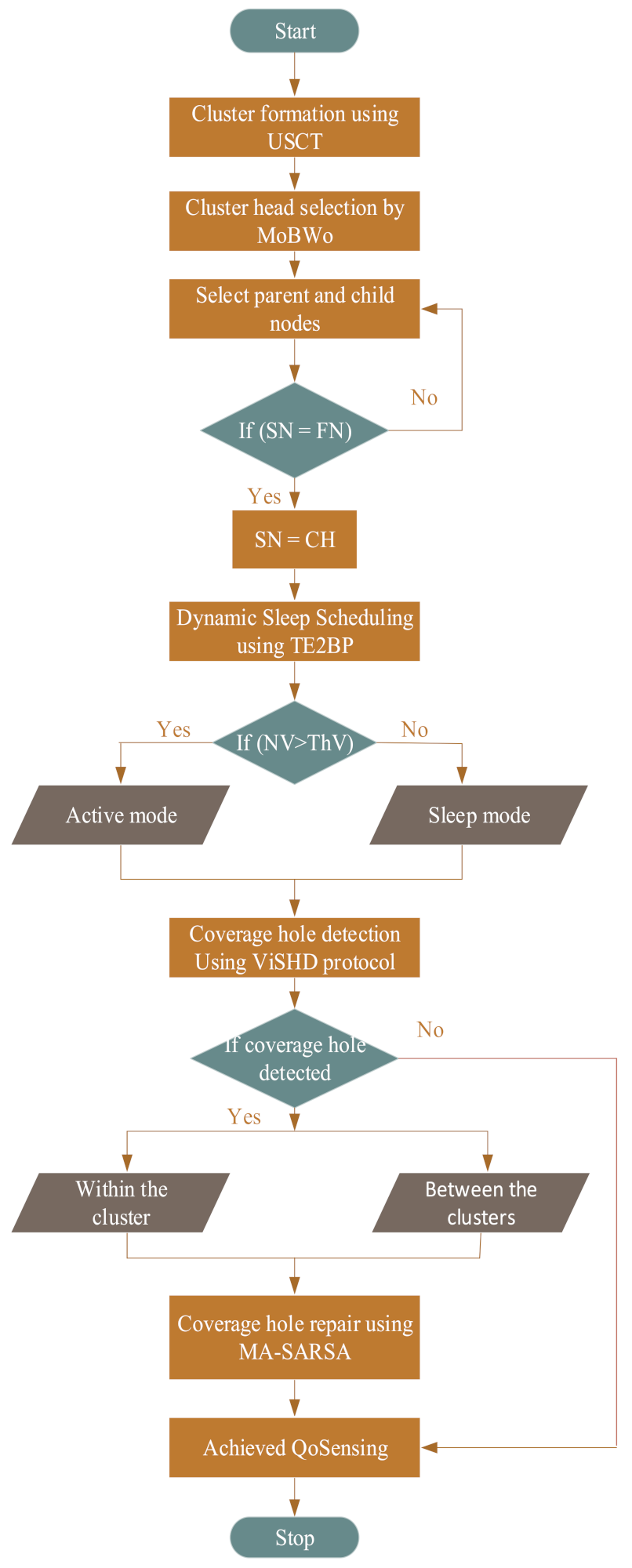Figure 4 depicts the overall flowchart of the proposed MiA-CODER approach.

Algorithm 4 Coverage hole repair

Initialization of Q($\mathit{\zeta },\mathit{\alpha })$ in a randomly;

For each trial repeat:

Initialization of $\mathit{\zeta }, \mathit{\alpha };$

For each trial step repeat:

Perform $\mathit{\alpha },$ obtain $\mathit{\gamma }$, ${\mathit{\zeta }}^{\prime }$;

Choose ${\mathit{\alpha }}^{\prime }$ from ${\mathit{\zeta }}^{\prime }$ using policy;

$\hspace{1em}\hspace{1em}\mathit{Q}\left(\mathit{\zeta },\mathit{\alpha }\right)\leftarrow \left(\mathbf{1}-{\mathit{\theta }}_{\mathit{\zeta }\mathit{\alpha }}\right)\mathit{Q}\left(\mathit{\zeta },\mathit{\alpha }\right)+{\mathit{\theta }}_{\mathit{\zeta }\mathit{\alpha }}(\mathit{\gamma }+\underset{{\mathit{\alpha }}^{\prime }}{\mathbf{max}}\mathbf{Q}\left({\mathit{\zeta }}^{\prime },{\mathit{\alpha }}^{\prime }\right));$

$\mathit{\zeta }\leftarrow {\mathit{\zeta }}^{\prime };\mathit{\alpha }\leftarrow {\mathit{\alpha }}^{\prime };$

Until $\mathit{\zeta } \mathit{t}\mathit{e}\mathit{r}\mathit{m}\mathit{i}\mathit{n}\mathit{a}\mathit{t}\mathit{e}\mathit{s}$

Until coverage hole is recovered

5. Experimental Results

In this section, the experimentation of the proposed coverage hole detection and recovery for achieving better QoSensing is carried out by using simulations. This section comprises of three sub-sections namely simulation setup, comparative analysis and research highlights in which the validation of the proposed model takes place in an elaborative manner.

5.1. Simulation Setup

The validation of the proposed model is executed in network simulator tool version 3.26. The hardware and software requirements for the purpose of simulation are provided in

Table 4. System configuration.

Hardware Specifications	Processor	NS3.26
	RAM	8 GB
	Hard Disk	60 GB
Software Specifications	Network Simulator	Pentium Dual Core and Above
	OS	Ubuntu 14.04 LTS

. The static sensor nodes, mobile sensor nodes and base station are deployed for the purpose of experimentation of the proposed model. The simulation of the proposed coverage hole detection and recovery is performed in 1000 × 1000 environment. The parameters required for the simulation are illustrated in

Table 5. Simulation parameters.

Parameters	Description
Simulation area	1000 m × 1000 m
Number of static nodes	25
Number of mobile nodes	50
Number of base stations	1
Sensing range	35 m
Data acquired bytes	1 KB
Number of bits transmitted	450 bits
Duration of single operation	0.140$\mathsf{\mu }\mathrm{s}$
Rmax	50 m
Pmax	300 mW
Path loss exponent	1
Hole size	80 m2
Energy	1 J
Simulation time	150 s
Queue length	10,000 packets
Node placement	Uniformly Random
Simulation rounds	1000
Network interface type	Physical wireless
Packet carry duration	1 s
Neighbor wait duration	0.5 s
Algorithm Parameters
SARSA
Epsilon	1
Learning rate	0.8
Discount factor	0.8
Decay	0.6

. The sensing range of the nodes is set to 35 m and the data acquired bytes are taken as 1 KB. The length of bits is considered as 450 bits. The Rmax refers to maximum sensing range and Pmax refers to power at maximum sensing range, respectively. The size of the coverage hole is taken as 80 m². The initial energy is of the sensor nodes is 1 J.

5.2. Comparative Analysis

The proposed coverage hole detection and recovery mechanism for better QoSensing is validated in this sub-section using various performance metrics. The efficiency of the proposed mechanism is proven by comparing it with several existing works. The performance metrics such as coverage rate, number of dead nodes, average energy consumption and throughput are considered for the evaluation.

5.2.1. Impact of Coverage Rate

The coverage rate refers to the amount of area covered by the sensor nodes in the region. In Figure 5, the coverage rate of the proposed MiA-CODER mechanism is compared with other existing research works with respect to the number of sensor nodes. The figure makes it clear that the coverage rate and number of sensor nodes are directly proportional to each other, which means that as the number of sensor nodes in the region increases the coverage rate also increases. The coverage rate of the proposed work is high as it performs both hole prevention and hole repair processes. The hole prevention is carried out by increasing the energy efficiency of the nodes and the hole repair is implemented by executing the multi-agent SARSA algorithm in which the base station covers the hole by moving the mobile node. The existing works perform either hole prevention or hole detection which are not efficient to achieve higher coverage rate.

Figure 6 depicts the comparison of the proposed MiA-CODER mechanism and several existing works in terms of coverage rate with respect to the simulation time. From the figure, it is clear that the coverage rate is inversely proportional to the simulation time which means that as the simulation time increases the coverage rate decreases eventually. The formation of cluster-tree topology using the Sierpinski triangle increases the energy efficiency of the sensor nodes which prevents the formation of coverage holes in the network. Further, the hole repair process performed by the base station eliminates the holes resulting in better QoSensing. The lack of implementation of both hole prevention and hole repair reduces the coverage rate of these approaches.

Table 6. Quantitative analysis of coverage rate.

Method	# of Sensor Nodes	Simulation Time (s)
MiA-CODER	94.95 $\pm$ 0.5	94.26 $\pm$ 0.5
SRC	83 $\pm$ 0.5	86.2 $\pm$ 0.5
H3	77.35 $\pm$ 0.5	81.4 $\pm$ 0.5

illustrates the coverage rate analysis of the proposed system with respect to other existing methods in terms of both number of sensors and simulation time. The overall coverage rate of the proposed approach is high when compared to other methods.

5.2.2. Impact of Number of Dead Nodes

The dead nodes refer to the nodes which are exhausted out of energy due to the inefficient management of the energy by the sensor nodes. In Figure 7, the number of dead nodes of the proposed MiA-CODER mechanism is compared with various existing works with respect to simulation time. The figure makes it clear that the simulation time and number of dead nodes are directly proportional to each other which means that as the simulation time increases the number of dead nodes also increases. The proposed mechanism has a low number of dead nodes than existing works because of the implementation of the unequal cluster topology and dynamic duty cycling of nodes in the network. The unequal cluster topology improves robustness and reduces the hotspot problem for the nodes near the base station. The execution of duty cycling reduces the unwanted wastage of energy in the network. The existing works have ineffectual topology structures and inefficient management of energy in the network.

In

Table 7. Number of dead nodes analysis.

Method	Simulation Time (s)
MiA-CODER	22 $\pm$ 1.0
SRC	30 $\pm$ 1.0
H3	38 $\pm$ 1.0

, the analysis of the number of dead nodes is presented for the proposed MiA-CODER mechanism with respect to other existing methods in terms of simulation time. The number of dead nodes is lower in the proposed method than in other approaches. This shows that the lifetime of the nodes is increased by our approach.

5.2.3. Impact of Average Energy Consumption

The average energy consumption refers to the average amount of energy consumed by the nodes in the network. The greater the energy consumption, the faster the nodes get exhausted. In Figure 8, the average energy consumption of the proposed work is compared with the existing works with respect to simulation time. From the figure it is clear that the simulation time and average energy consumption are directly proportional to each other. The average energy consumption of the proposed MiA-CODER mechanism is low compared to other existing works due to the implementation of Sierpinski triangles-based unequal clustering and sleep scheduling of nodes in the network. This reduces the energy consumption of the nodes in the network thereby increasing the lifetime of the nodes. The existing approaches do not provide an efficient energy consumption mechanism which increases the energy consumption of the nodes and reduces the lifetime of the network.

5.2.4. Impact of Throughput

Throughput in the wireless sensor network is defined as the measure of the amount of data that can be received in a certain amount of time. In Figure 9, the throughput of the proposed work is compared with several existing works with respect to the number of sensor nodes.

Figure 9 makes it clear that the throughput increases with the increase in the number of sensor nodes. The throughput of the proposed MiA-CODER mechanism is high due to the detection and coverage of holes in the network. The detection of holes is carried out by the virtual sector-based hole detection protocol (ViSHD) and the recovery of coverage holes is executed by implementing the multi-agent SARSA based on multiple parameters. The existing works lack proper recovery mechanisms which affect the throughput of those approaches.

5.2.5. Impact of Reliability

Reliability is defined as the measure of the total number of packets successfully transmitted and received in the network during a certain period of time. It proves the efficiency of a mechanism in the long run. The reliability of the proposed MiA-CODER mechanism is compared with that of other approaches in terms of simulation time. It is found that the packet transmission and reception rate increase with the increase in the simulation time. For a mechanism to be stated as highly reliable, the number of transmitted packets, number of received packets and number of control packets should be high. The reliability of an approach is affected by the coverage holes which are formed in the network. The reliability of the proposed MiA-CODER mechanism is analyzed both before and after coverage hole repair.

5.2.6. Reliability before Coverage Hole Repair

In Figure 10, the number of transmitted packets for the proposed MiA-CODER mechanism before coverage hole repair is compared with other existing approaches with respect to the simulation time. The proposed MiA-CODER mechanism has a high number of successful transmitted packets even before coverage hole repair due to the adoption of coverage hole prevention. This reduces the number of coverage holes formation in the network. In particular, the proposed mechanism is found to be reliable during the 150th second of simulation time with a maximum number of transmitted packets compared to other approaches. The existing approaches have reduced the number of successful transmitted packets due to the lack of coverage prevention techniques.

Figure 11 presents the comparison of the proposed MiA-CODER mechanism before coverage hole repair with several existing works in terms of the number of successfully received packets with respect to the simulation time. The proposed mechanism is found to have the maximum number of successfully received packets due to the implementation of the unequal cluster-tree topology and effective selection of cluster head using the MoBWo algorithm. The number of packets received successfully is low for the existing approaches because they provide solutions only for coverage holes detection and repair but not for the prevention of coverage holes in the network.

The comparison of the proposed MiA-CODER mechanism with other existing works in terms of the number of control packets before coverage hole repair with respect to simulation time is presented in Figure 12. The proposed mechanism has a high number of control packets due to the formation of unequal Sierpinski cluster-tree topology (USCT) and the implementation of dynamic sleep scheduling in the network. This reduces the load in the network, thereby facilitating the effective transmission of data. The existing approaches did not focus on proper management of the load in the network which affects the reliability of those approaches.

5.3. Reliability after Coverage Hole Repair

The number of transmitted packets for the proposed MiA-CODER mechanism after coverage hole repair is compared with other existing approaches with respect to the same simulation time. By comparing Figure 10 and Figure 13 it is clear that the number of transmitted packets of the proposed MiA-CODER mechanism is increased after the coverage hole repair, thereby resulting in improved reliability. This is due to the implementation of coverage hole detection and repair in which the coverage hole is detected by the CH using the virtual sector-based hole detection (ViSHD) protocol in which the coverage holes both within the cluster and among the clusters are detected. Furthermore, the coverage hole repair is carried out by the BS using the MA-SARSA algorithm in which the coverage hole is repaired by selecting an optimal mobile node nearer to the hole and replacing it in the hole region. By doing so, the efficient transmission of data is achieved, thereby resulting in improved QoSensing in the network. The lack of efficient coverage hole detection and repair strategies affects the reliability of the existing approaches.

The number of received packets of the proposed MiA-CODER mechanism after coverage hole repair is compared with other existing works with respect to the simulation time. From Figure 11 and Figure 14 it is clear that the number of received packets increased after the coverage hole repair resulting in increased reliability to the approach. This is due to the detection of coverage holes and repair of coverage holes in an efficient manner resulting in effective reception of data, thereby achieving improved QoSensing.

The comparison of the proposed MiA-CODER mechanism with various existing methods after coverage hole repair with respect to the simulation time is provided in Figure 15. It can be said that the number of control packets increases after the coverage hole repair which means that the execution of coverage hole repair increases the reliability of the proposed mechanism. The increase in the number of control packets is due to the efficient coverage hole detection and repair carried out by the proposed mechanism. The detection of coverage holes both inside the cluster and between the clusters improves the accuracy of the hole detection process which helps in the recovery of the coverage holes through an effective hole repair mechanism. Hence, the reliability of the proposed mechanism is higher than the existing approaches.

5.4. Research Highlights

• The network environment is constructed as an unequal Sierpinski cluster-tree topology (USCT) in order to eliminate the hotspot problem by increasing the energy efficiency of the network.
• The cluster head is elected in an optimal manner by implementing multi-objective black widow optimization (MoBWo) in order to facilitate effective transmission of data in the network.
• The energy efficiency of the nodes in the network is further improved by scheduling the sensor nodes between active and sleep mode using Tsallis entropy enabled Bayesianprobability (TE2BP) based on several significant factors.
• The coverage holes in the network are detected by executing virtual sector-based hole detection (ViSHD) in which the holes are detected by the CH both within the cluster and among the clusters.
• The QoSensing of the network is improved by performing a recovery process in which the base station repairs the coverage holes by implementing multi-agent SARSA (MA-SARSA) based on important parameters.

6. Conclusions and Future Work

In this paper, the QoSensing of the wireless sensor network is improved by enhancing the coverage in the network. This is executed by proposing the MiA-CODER mechanism. Initially, the energy consumption of each node is minimized by performing the unequal Sierpinski cluster-tree topology (USCT) in which the network area is divided into unequal triangles in such a way that the triangle nearer to the base station will be larger, thereby consuming less energy in order to eliminate the hotspot problem. From each cluster, the most efficient node based on energy distance and capacity is selected as the CH by implementing multi-objective black widow optimization (MoBWo). Further, the energy consumption in the network is minimized by performing dynamic sleep scheduling by implementing Tsallis entropy enabled Bayesian probability (TE2BP) in which the probability of the node to be in either sleep mode or active mode is computed based on the entropy value for significant parameters. Due to the minimization of energy consumption in the network, the possibility of the occurrence of hole coverage is less; however, in the case of the network facing a coverage hole problem, the coverage holes are detected by performing the virtual sector-based hole detection (ViSHD) protocol in which the virtual sectors are constructed and the hole detection is carried out by the CH both within the cell and among the cells. Once the hole is detected accurately, the BS executes the multi-agent SARSA algorithm in which the hole repair process is carried out by optimally selecting a mobile node to cover the hole which is completed based on distance, lifetime and coverage level. This enhances the coverage, thereby improving QoSensing in the network. The proposed MiA-CODER approach is experimented with in the network simulator NS 3.26 tool and the efficiency of this approach is proven by comparing it with several existing approaches in terms of coverage rate, number of dead nodes, average energy consumption and throughput. In the future, the proposed coverage hole detection and repair mechanism is to be improved in security aspects and evaluated in a real-time IoT environment.