Application of an Automatic Noise or Signal Removal Algorithm Based on Synchrosqueezed Continuous Wavelet Transform of Passive Surface Wave Imaging: A Case Study in Sichuan, China

Abstract

Passive surface wave imaging based on noise cross-correlation has been a research hotspot in recent years. However, because randomness of noise is difficult to achieve in reality, prominent noise sources will inevitably affect the dispersion measurement. Additionally, in order to recover high-fidelity surface waves, the time series input during cross-correlation calculation is usually very long, which greatly limits the efficiency of passive surface wave imaging. With an automatic noise or signal removal algorithm based on synchrosqueezed continuous wavelet transform (SS-CWT), these problems can be alleviated. We applied this method to 1-h passive datasets acquired in Sichuan province, China; separated the prominent noise events in the raw field data, and enhanced the cross-correlation reconstructed surface waves, effectively improving the accuracy of the dispersion measurement. Then, using the conventional surface wave inversion method, the shear wave velocity profile of the underground structure in this area was obtained.

1. Introduction

Passive seismic methods do not require the excitation of explosives, vibroseis, etc.; they simply require the placement of node geophones according to the active source acquisition line and point spacing, and the data can be collected by continuously receiving ambient noises. Then, by using seismic interferometry (SI), the responses of virtual sources can be retrieved through the correlated responses on the two receivers [1,2,3,4]. The term “interferometry” generally refers to the study of interference between signals in order to obtain information through the differences between them. In the field of SI, it is used to study the interference of seismic-related signals. Its basic operation steps are very simple, mainly divided into two steps: the first step is cross-correlation calculation, which can be understood as detecting the travel time difference of waves recorded between two receivers; the second step is stacking—that is, integrating all actual sources.

Although the theory of SI is not limited to either body or surface waves [5,6], extracting surface waves from the cross-correlation of ambient noise is quite robust and has become a mature technology [7]. In contrast, it is much more difficult to extract body waves [8,9]. However, some studies have also shown its possibility at various scales [10,11,12,13]. Even so, in most SI studies, retrieving surface waves is still one of the major applications. Surface waves with different periods can be used to investigate the earth structure at different depths [14]. Generally speaking, most studies focus on frequencies lower than 1 Hz to provide images of the structure of the crust and upper mantle [15,16]. However, some studies have proven that structures tens to hundreds of meters underground can be imaged with frequencies higher than 1 Hz, such as by using traffic noise to detect urban underground space [17,18], which has attracted the attention of more and more engineering seismologists.

Green’s function reconstruction of diffuse wavefield (i.e., waves arrive from all angles with equal strength) observations in an open configuration is the basis for SI with passive data [19]. However, it is not realistic to obtain a pure diffuse wavefield from observations. Non-ideal source distributions such as limited azimuthal distribution or near-source effects [20] can significantly affect the reliability and interpretation of observations due to the violation of the stationarity assumptions required by passive survey methods [21]. In order to improve the accuracy of the dispersion measurement, some studies have begun to consider how to attenuate the influence of noise sources with prominent directivity. Aki [5] proposed a classical spatial autocorrelation method which used the mathematical transformation of a symmetric receiving array (e.g., circle) to eliminate the azimuth factor of the noise source. Park et al. [22] introduced a novel strategy for imaging dispersion of passive surface waves with an active scheme based on phase-shift measurement, called roadside passive multichannel analysis of surface waves. Scanning processes were implemented along potential azimuthal directions of noise. Feuvre et al. [23] proposed a cross-correlation-based beamforming average dispersion analysis method which effectively restrained the directionality of noise and reduced the aliasing effect. Cheng et al. [24] proposed a multichannel analysis of the passive surface (MAPS) wave method based on long noise sequence cross-correlation to handle the azimuthal effects for directional noise sources. Distinct from the above methods, Mousavi et al. [25] proposed a new and fast algorithm for accurate noise removal/signal removal based on higher-order statistics (HOS), general cross-validation (GCV), and wavelet hard thresholding (WHT) in synchrosqueezed domains and tested the performance of the proposed algorithm with synthetic and real seismic data. In addition, he indicated that it can also be an effective procedure in ambient noise studies.

In this paper, we applied the noise or signal removal algorithm based on SS-CWT proposed by Mousavi et al. [25] to a 1-h passive seismic dataset acquired in Sichuan, China, and verified the effectiveness of this method in enhancing passive surface waves from short time series. First, we used this method to preprocess the 1-hour passive seismic data in Sichuan to remove the prominent noise events and used cross-correlation to produce virtual shot gathers from the preprocessed noise records. Then, after cross-correlation, the method was used as a post-processing step to denoise the virtual shot gathers, improving the signal-to-noise ratio (S/N) of the virtual shot gathers and further improving the reconstructed surface waves. Next, after preprocessing and post-processing, virtual shot gathers were used for dispersion analysis with an active scheme based on the phase-shift measurement, and inversion was conducted to obtain the underground shear wave velocity profile in this area. Finally, the applicability and shortcomings of this method are discussed.

2. Methodology

The methodology used in this paper was proposed by Mousavi et al. [25]. We summarized and sorted out their methods, mainly including the following three processing steps.

2.1. Preprocessing

For the passive seismic data $y$ collected in the field, first, we carried out CWT and calculated its coefficient $W_y$, which represents the finite energy of the data in a concentrated time–frequency picture. CWT is a multiresolution transform method given by [26], as shown in Equation (1):

$$W_y\left(a,\tau \right)=⟨y,{\psi }_{a,\tau }⟩={\int }_{-\infty }^{+\infty }y\left(t\right)a^{{-}_2^1}{\psi }^{\ast }\left(\frac{t-\tau }{a}\right)dt,$$

(1)

where $a$ and $\tau$ denote the scale and time shift, respectively; $\ast$ is the complex conjugate; $y,\psi$ denotes the inner product; and $\psi$ is the mother wavelet.

Then, we used HOS and the kurtosis criterion to detect the scale of and remove the pure Gaussian noise correlation coefficient from the time–frequency analysis (TFR), leaving the combination of noise and signal. The $Kurt$ of $N$ observation coefficients $W_y$ can be calculated by Equation (2):

$$Kur{t}_y=\frac{{\sum }_{n=1}^N{\left(W_{y_n-}{\mu }_{W_y}\right)}^4}{N{\sigma }_{W_y}^4}-3,$$

(2)

where ${\sigma }_{W_y}$ and ${\mu }_{W_y}$ are the estimated standard deviation and mean value of wavelet coefficient $W_y$, respectively, and $N$ denotes the sample sequence. HOS measure the degree of Gaussianity, so they have been used as detectors of non-Gaussian signals in Gaussian noise [27]. Equation (3) defines the HOS criterion, which is retained for the Gaussianity measure for distinguishing Gaussian distributions from non-Gaussian distributions:

$$\left|Kur{t}_y\right|\le \frac{\sqrt{24/N}}{\sqrt{1-\alpha }},$$

(3)

where $\alpha$ is the level of confidence. Ravier et al. [28] estimated that the optimal value of $\alpha$ is 90%.

2.2. Thresholding

After obtaining the processed coefficient $W_y$ through the preprocessing steps, the synchrosqueezed transform was performed according to Equation (4) to obtain the synchrosqueezed-CWT (SS-CWT) coefficients $T_y$.

$$T_y\left({\omega }_{\ell },\tau \right)=\mathsf{\Delta }{\omega }^{-1}{\displaystyle \sum }_{a_k\left|\omega \left(a_k,\tau \right)-{\omega }_{\ell }\right|\le \frac{\mathsf{\Delta }\omega }{2}}{W}_y\left(a_k,\tau \right)a_k{}^{-\frac{3}{2}}\mathsf{\Delta }{a}_k,$$

(4)

where $\omega$ is the discrete frequency and ${\omega }_{\ell }$ represents the $\ell$th discrete frequency, $a_k$ represents the $k$th scale, $\tau$ is the time shift, and $\mathsf{\Delta }$ represents the increment symbol, where $\mathsf{\Delta }\mathrm{a}=a_k-a_{k-1}$.

Then, we used the hard threshold scheme (Equation (5)) proposed by Donoho et al. [29,30] to provide a threshold for the SS-CWT coefficients $T_y$.

$${\mathsf{\eta }}_{\mathsf{\lambda }}^h\left(W_y,\mathsf{\lambda }\right)=\{\begin{array}{c}{W}_y ,\left|W_y\right|>\mathsf{\lambda }\\ 0 ,\left|W_y\right|<\mathsf{\lambda }\end{array},$$

(5)

where $\mathsf{\lambda }$ is the selected appropriate threshold; $\mathsf{\eta }$ is the selected threshold rule, which can be divided into a hard threshold and a soft threshold; ${\mathsf{\eta }}_{\mathsf{\lambda }}^h$ represents the hard threshold rule; and $W_y$ represents the wavelet coefficients of observation $y$.

The optimal threshold $\mathsf{\lambda }$ was automatically determined by the GCV method, which was proposed by Nason et al. [31]. The GCV function is defined as follows:

$$\mathrm{GCV}\left(\mathsf{\lambda }\right)=\frac{1}{N}\frac{\Vert T_y-{\tilde{T}}_{\mathsf{\lambda }}\Vert {}^2}{\Vert \frac{N_0}{N}{\Vert }^2},$$

(6)

where $\widetilde{T_{\mathsf{\lambda }}}$ is the threshold coefficient using the threshold $\mathsf{\lambda }$, and $N_0$ is the number of coefficients using the threshold $\mathsf{\lambda }$ to return to zero. This function simulated the error between the estimated signal and the real signal, so its minimum value was used to select an optimal threshold. By selecting thresholds for the main components of the signal, the initial estimation of the signal was obtained using Equation (7):

$$y_k\left(t\right)=2C_{\psi }^{-1}Re\left({\displaystyle \sum }_{l\in L_k\left(t\right)}{T}_y\left({\omega }_{\ell },t\right)\right),$$

(7)

where $L_{k\left(t\right)}$ denotes a small frequency band around the ridge of the $k$th component in the SS-CWT, the symbol $Re$ represents the real part, and the constant $C_{\psi }$ is given by Thakur et al. [32]:

$$C_{\psi }={\int }_0^{\infty }{\xi }^{-1}{\widehat{\psi }}^{\ast }\left(\xi \right)d\xi ,$$

(8)

where $\ast$ represents the complex conjugate; $\psi$ is the mother wavelet, which is a square integrateable function; $\xi$ is the angular frequency; and $\widehat{\psi }$ is the Fourier transform of $\psi$.

2.3. Postprocessing

In the third step, a simple level-dependent wavelet threshold was applied to the signal obtained in the thresholding steps; the initial estimation of the seismic signal was subjected to CWT, shown in Equation (1); and thresholds of the coefficients of all scales were selected step by step using the hard threshold rule again, as shown in Equation (5). However, the threshold $\mathsf{\lambda }$ estimation used here was given by Donoho et al. [29], which was calculated using Equation (9):

$$\mathsf{\lambda }={\sigma }_n\sqrt{2\ln N},$$

(9)

where ${\sigma }_n=median\left(\left|W_y\right|\right)/0.6745$. Finally, the signal in the original data was extracted by applying an inverse CWT, as shown in Equation (10):

$$y\left(t\right)=\frac{1}{C_{\psi }}{\iint }^{ }{W}_y\left(a,\tau \right)d\tau \frac{da}{a^2}.$$

(10)

For the passive seismic raw records, the extracted signal $y\left(t\right)$ represented the records that contained unnecessary prominent noise events, and the uniform background noise could be extracted by subtracting $y\left(t\right)$ from the original data $y$.

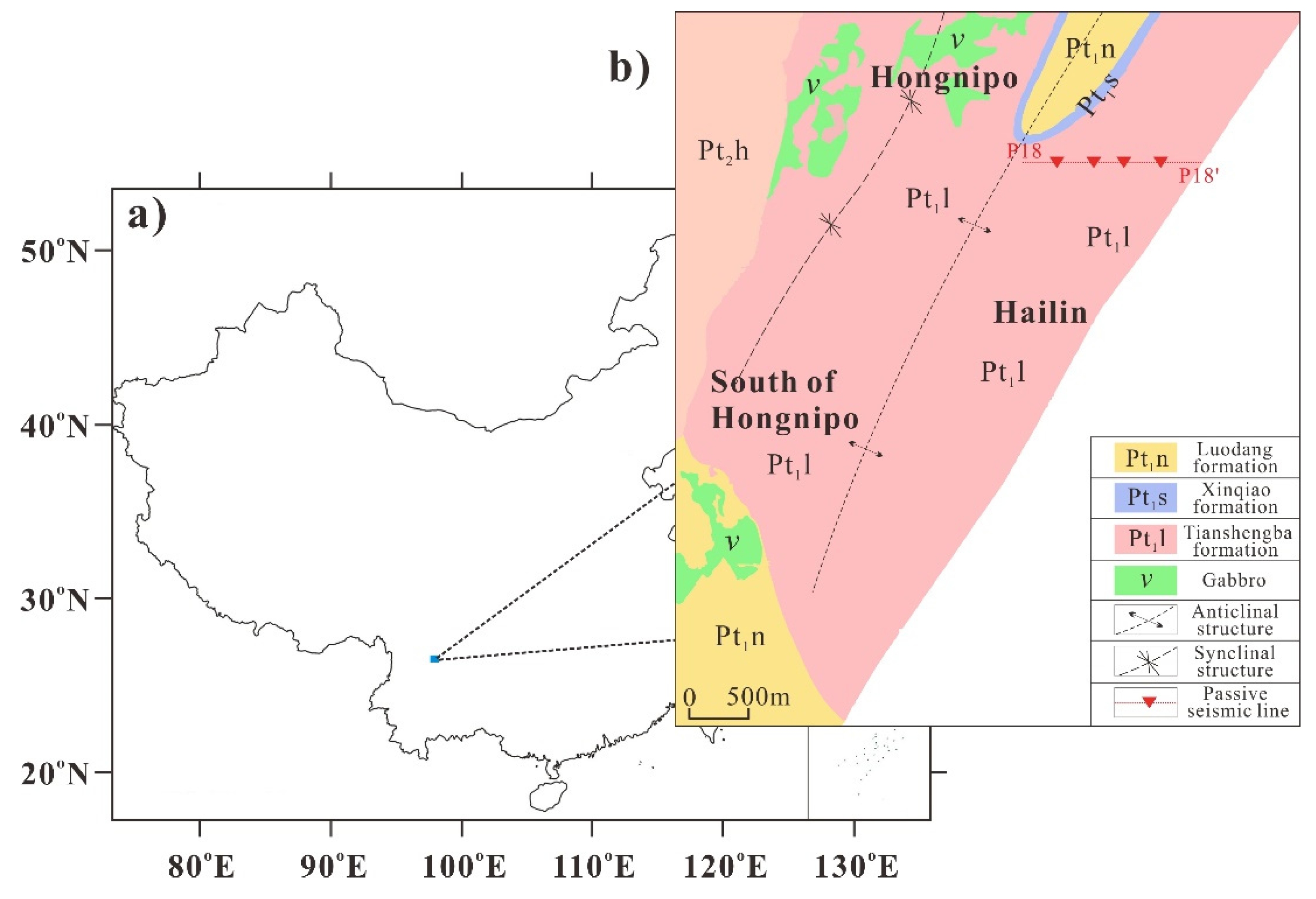
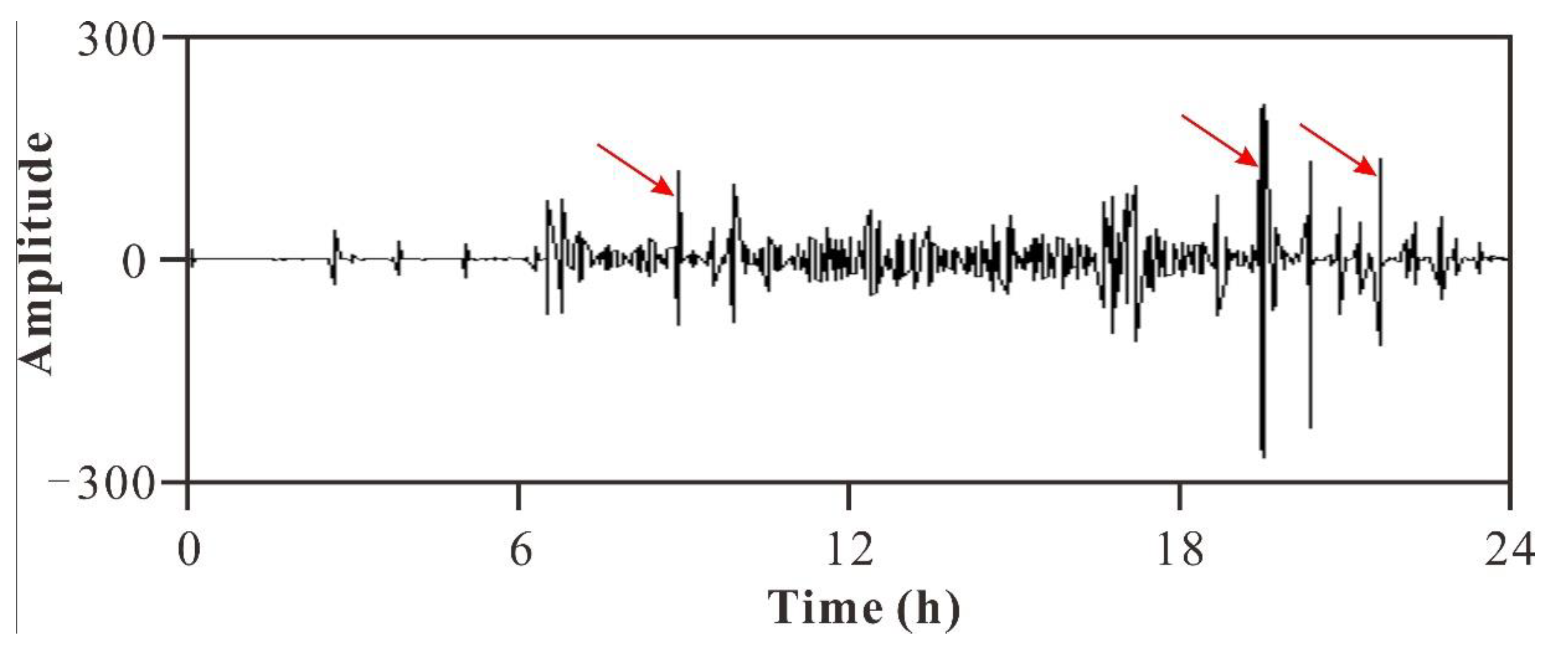
3. The Field Data

The passive seismic data acquisition area is located in a mining area in Sichuan (as shown in the blue square in Figure 1a), where Triassic feldspar quartz sandstone, Jurassic marl-dolomite-feldspar quartz sandstone, Cretaceous purplish red mudstone-siltstone- sandstone, and Quaternary strata are exposed. Figure 1b shows a diagram of the geological structure of the mining area. The main structural direction of this area is north–northeast, followed by nearly east–west. Magmatic rocks in the mining area are mainly gabbro and diabase from the late Jinning period, which are exposed as rock masses and dikes of different sizes. The wall rock alteration is developed, among which the wall rock alteration related to mineralization mainly includes chloritization, silicification, and carbonization.

We arranged a two-dimensional passive seismic survey line, P18-P18″, at the periphery of the mining area (as shown by the red dotted line in Figure 1b). The passive seismic data were continuously recorded for 4 days with a 1-millisecond sample interval using 120 node-type single-component geophone I-Nodal at 1-240 Hz natural frequency. The distance between each geophone was 12.5 m, and the total length of the survey line was 1.5 km. In order to avoid surface wind noise, the geophones were buried at depths of about 20 cm.

The maximum elevation difference of the terrain in the test area was 100 m, and the slope was gentle. The surrounding areas were sparsely populated and underdeveloped, with one or two village-level roads. There were many rivers nearby, and there were mining activities about 4 km northwest. Comprehensive analysis showed that the noise in this area mainly came from rivers, traffic, and mining activities, and mining activities may be the main source of prominent noise events. Figure 2 shows the daily noise data recorded by a geophone.

There was very little noise from night to morning (0–6 h), with relatively low amplitude and stable change, whereas during the day, due to activities such as surface mining, the noise amplitude was relatively high and changed drastically, including some prominent high-amplitude noise events (red arrows). Therefore, in order to satisfy the hypothesis of a theoretical wavefield as much as possible, the original field data were processed.

4. Field Data Processing

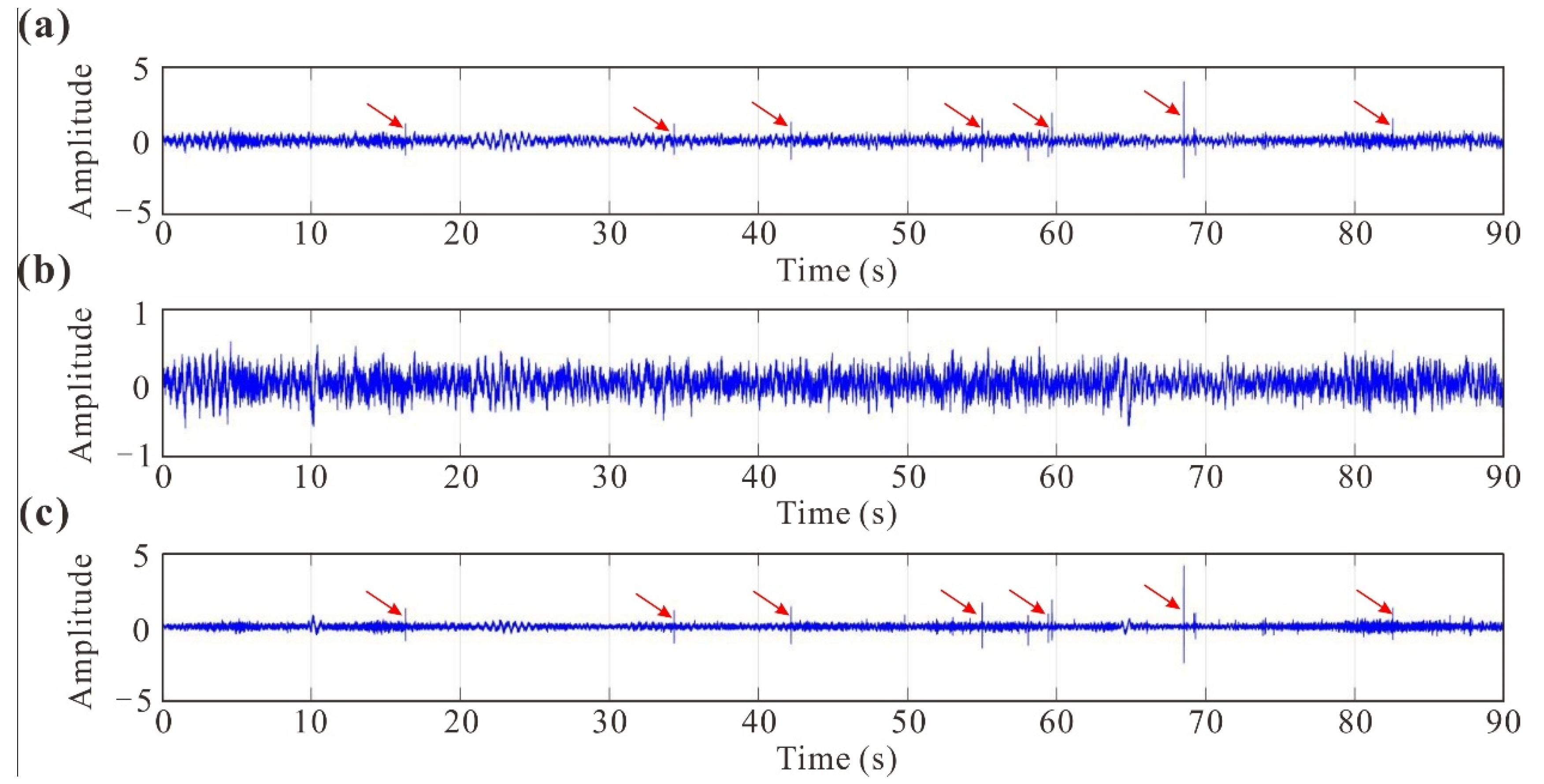
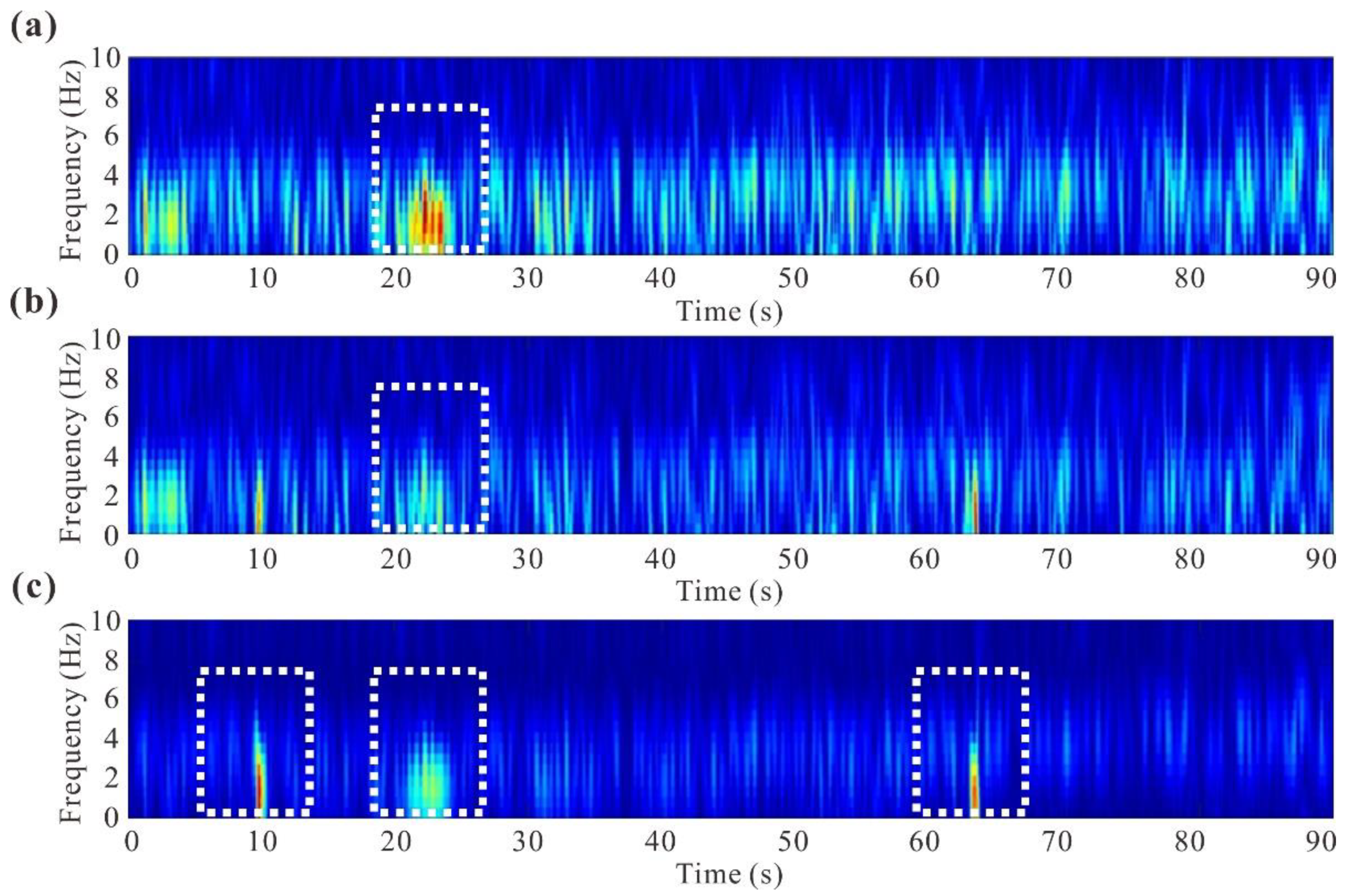
4.1. Preprocessing for Raw Field Data

Raw field data will inevitably be affected by prominent noise events (e.g., mechanical construction), which makes it impossible to satisfy the assumption of a diffuse wavefield. Therefore, in order to reconstruct passive surface waves better, we first used the noise or signal removal algorithm based on SS-CWT proposed by Mousavi et al. [25] to preprocess the field data and separate the prominent noise events. Figure 3a shows an original field record of 90 s on which several relatively prominent noise events (red arrows) are distributed. After noise and signal separation, the amplitude of the separated noise records was relatively evenly distributed (as shown in Figure 3b). Figure 3c shows the removed records containing prominent noise events (red arrows).

Power spectral density (PSD) plots are useful for visualizing variations in the frequency content of ambient data over time [33]. In order to further show the application effect of the noise separation algorithm in preprocessing the field data, we also calculated the PSD plots (as shown in Figure 4) corresponding to the three noise records in Figure 3.

Figure 4a shows the PSD plots of the original field data, on which a prominent high-energy event (white dotted box) can be seen. After noise separation, as shown in Figure 4b, the high-energy event in the white dotted box was attenuated, and the PSD of the whole record was evenly distributed. Figure 4c shows the PSD of the removed noise record, which was occupied by three prominent high-energy events (white dashed boxes). According to the results of Figure 3 and Figure 4, the noise or signal removal algorithm based on SS-CWT could effectively remove the prominent noise events in the original passive seismic data.

4.2. Reconstruction of Virtual Shot Gathers by Cross-Correlation

After preprocessing the raw field data, one geophone served as a virtual source for waves recorded by other receivers when using the cross-correlation calculation; thus, we could obtain all virtual shot gathers from every receiver without using an active source. In this paper, we showed the virtual shot gathered with the first receiver as the virtual source. In addition, in order to better characterize the intensity of the surface waves on the reconstructed virtual shot gathers, we used the dispersion curve image obtained by the phase-shift measurement method as the visualization tool.

Figure 5a shows the virtual shot gather formed by the cross-correlation of raw passive seismic data acquired in Sichuan for a certain hour. The surface waves (indicated by red arrows) can be seen in the red box on the virtual shot gather but are concealed by the energy of a strong transverse axis. The corresponding dispersion curve image is shown in Figure 5b, and the dispersion curve (red part) is disordered and discontinuous.

After preprocessing the raw field data, the virtual shot gather formed by the separated noise records is shown in Figure 6a. Compared with Figure 5a, the in-phase axis (indicated by the red arrow) of the internal surface waves in the red box for the processed virtual shot gather is clearer, but it is still concealed by the energy of the strong horizontal axis. The corresponding dispersion curve image is shown in Figure 6b, where the curve (red part) is clearer and more continuous than in Figure 5b.

By comparing the virtual shot gathers and their corresponding dispersion curve images in Figure 5 and Figure 6, we saw that the virtual shot gather formed by the separated noises had clearer surface wave in-phase axes and dispersion curves, which proved that the noise or signal removal algorithm based on SS-CWT could effectively enhance the reconstructed surface waves after preprocessing the raw field data.

4.3. Post-Processing for Virtual Shot Gathers

Although preprocessing the raw field data before cross-correlation could effectively enhance the surface waves, the surface waves on the virtual shot gather were still concealed by the strong transverse axis energy. Determining how to eliminate the strong transverse axis energy, improve the S/N of the virtual shot gather, and further enhance the surface waves is of great significance for subsequent inversion and imaging.

Baig et al. [34] proposed several methods to improve the fidelity of noise cross-correlation based on the discrete orthogonal S transform, which showed that time–frequency denoising of correlograms (i.e., virtual shot gathers) can alleviate this problem. The noise or signal removal algorithm based on SS-CWT proposed by Mousavi et al. [25] can also be applied to the virtual shot gather after cross-correlation to denoise correlograms and improve the S/N. Figure 7 shows the virtual shot gather (Figure 7a) and its dispersion curve image (Figure 7b) after denoising the correlogram of Figure 5a using the noise or signal removal algorithm based on SS-CWT. Comparing Figure 7a with Figure 5a, the strong transverse axis energy on the correlogram was effectively eliminated, and the surface waves were highlighted. The dispersion curve in Figure 7b (red part) is more concentrated and continuous than that in Figure 5b.

The above research showed that the noise or signal removal algorithm based on SS-CWT could effectively enhance the surface waves after preprocessing the raw field data. At the same time, the method could also denoise the correlogram to further enhance the surface waves. Therefore, for the passive seismic datasets acquired in Sichuan, we first preprocessed the raw field data, then used the separated noise records to perform cross-correlation calculations to form the virtual shot gathers, and finally post-processed the correlograms, thus obtaining the final virtual shot gather, shown in Figure 8a, and its corresponding dispersion curve image (Figure 8b).

Comparing Figure 8 with Figure 5, Figure 6 and Figure 7, we observed that the strong transverse axis energy in the virtual shot gather (Figure 8a) was eliminated, and the surface waves were richer and clearer; the information of the low-frequency part in the dispersion map shown in Figure 8b is prominent, and the dispersion curve is clear and continuous.

4.4. Shear Wave Velocity Profile

According to the pre- and post-processing steps mentioned above, we obtained virtual shot gathers with each receiver as the virtual shot point. We used phase-shift measurement for dispersion analysis and then used the genetic algorithm [35] to invert the underground shear wave velocity structure.

The genetic algorithm is an efficient, parallel, random global optimization search algorithm based on biological genetic mechanisms and natural selection. It searches for the optimal solution by giving a hypothetical solution and simulating the process of natural evolution. This method has been widely promoted and successfully applied in many fields, and it is also a commonly used Rayleigh wave dispersion curve inversion method. The initial model parameters (i.e., hypothetical solution) and the inversion parameters are shown in

Table 1. Initial model parameters and the parameters used for inversion by genetic algorithm.

Parameters Used to Constrain the Initial Model				Parameters Used for Inversion
Layer Number	Lower Limit of Shear Wave Velocity (m/s)	Upper Limit of Shear Wave Velocity (m/s)	Layer Thickness (m)	Vp/Vs	Density (kg/m3)	Number of Iterations
1	200	400	10	2	2	10,000
2	400	500	20
3	500	600	30
4	600	800	50
5	800	1000	90

.

In Figure 9, we show the inversion result of the dispersion curve in Figure 8. Figure 9a shows the initial picked dispersion curve (red dotted line) and the inverted dispersion curve (blue line), and Figure 9b shows the given upper and lower limits of the initial shear wave velocity model (red dotted line) and the inverted underground shear wave velocity structure (blue line). The high-frequency component of the surface wave mainly reflects the shallow underground information, while the low-frequency component mainly reflects the deep underground information. As there were few or no dispersion data recorded by the passive seismic data in the low-frequency range (1–2.5 Hz), the inversion results of the shallow part (0–200 m in Figure 9b) of the shear wave velocity structure are more accurate, while the inversion results of the deep part (200–300 m in Figure 9b) are not necessarily the same. Therefore, the depth range of the finally inverted shear wave velocity profile is 0–200 m underground.

We then selected the virtual shot gathers at 30 receivers, used phase-shift measurement for dispersion analysis, and obtained the inverse shear wave velocity structures of those 30 receivers. Finally, the shear wave velocity structure profile in this area was obtained by Kriging interpolation [36], as shown in Figure 10; the red inverted triangle indicates the position of the inverted shear wave velocity structure, and the section length of the final inversion is 1300 m. As the data quality of the following (1300–1500 m) is poor, it cannot avoid bringing errors to the whole inversion, so it was abandoned. Its underground structure is clear, and there is a fault, F, at approximately 900 m.

5. Discussion

Although the noise or signal removal algorithm based on SS-CWT proposed by Mousavi et al. [25] has achieved outstanding results in this case study, there are still some problems that need further discussion. In this section, we highlight two issues based on our experience of processing the Sichuan passive seismic dataset: (1) the applicability of this method in other passive seismic datasets, and (2) the efficiency of this method in processing passive seismic datasets.

5.1. The Applicability of This Method in Other Passive Seismic Datasets

Due to differences in collection environment and conditions, there are often great differences between different passive seismic datasets. Therefore, in addition to testing the passive seismic dataset in Sichuan, we also attempted to apply this method to a passive seismic dataset acquired in Inner Mongolia [37] to enhance the surface waves but did not achieve very obvious results. As the survey line arranged in the research area of Inner Mongolia was located near a village, and it was the busy farming season, when farmers used agricultural machinery to harvest corn in the field, the human activities were complex and the interference was serious, so this method might not be able to completely eliminate these complex noises. However, the study area in this paper is far away from the village, with little human interference, and only the mining activities about 4 km northwest of the survey line are prominent. Therefore, although this method had a good effect in processing the Sichuan dataset, it may not have obvious effects on the datasets collected in different environments (especially in areas where human activities are prominent).

5.2. The Efficiency of This Method in Processing Passive Seismic Datasets

The amount of passive seismic data was relatively large. Taking the Sichuan dataset as an example, the amount of data collected by 120 geophones for 1 ms was approximately 40 GB a day. When we used this method to process the 1-h data selected by each receiver, it took more than 20 min to preprocess each trace, and it took 40 h to complete the whole 1-h dataset of 120 receivers; thus, the calculation efficiency was relatively low. Therefore, further improvement of this method for calculation efficiency is required before applying it to larger passive seismic datasets.

6. Conclusions

We introduced an accurate noise or signal removal algorithm based on SS-CWT. The performance of this algorithm was tested with actual passive seismic data acquired in a certain area of Sichuan, China. The results show that this algorithm can not only eliminate unnecessary prominent coherent noise events in the original passive seismic data but can also denoise the correlogram formed after cross-correlation calculation, improve the S/N of the restored Green function, and enable the reconstruction of a high-fidelity Green function from short time series. However, the computational efficiency of this method is low, and it may not be able to achieve good application results on datasets that are greatly disturbed by human activities.

References

- Wapenaar, K. Retrieving the elastodynamic Green’s function of an arbitrary inhomogeneous medium by crosscorrelation. Phys. Rev. Lett. 2004, 93, 254–301. [Google Scholar] [CrossRef] [Green Version]
- Schuster, G.T.; Yu, J.; Sheng, J.; Rickett, J. Interferometric/daylight seismic imaging. Geophys. J. Int. 2004, 157, 838–852. [Google Scholar] [CrossRef]
- Weaver, R.L. Information from Seismic Noise. Science 2005, 307, 1568–1569. [Google Scholar] [CrossRef] [Green Version]
- Snieder, R.; Şafak, E. Extracting the building response using seismic interferometry: Theory and application to the Millikan library in Pasadena, California. Bull. Seismol. Soc. Am. 2006, 96, 586–598. [Google Scholar] [CrossRef] [Green Version]
- Aki, K. Space and time spectra of stationary stochastic waves, with special reference to microtremors. Bull. Earthq. Res. Inst. 1957, 35, 415–456. [Google Scholar]
- Claerbout, J.F. Synthesis of a layered medium from its acoustic transmission response. Geophysics 1968, 33, 264–269. [Google Scholar] [CrossRef]
- Nakata, N.; Snieder, R.; Tsuji, T.; Larner, K.; Matsuoka, T. Shear-wave imaging from traffic noise using seismic interferometry by cross-coherence. Geophysics 2011, 76, SA97–SA106. [Google Scholar] [CrossRef] [Green Version]
- Roux, P.; Sabra, K.G.; Gerstoft, P.; Kuperman, W.A. P-waves from cross-correlation of seismic noise. Geophys. Res. Lett. 2005, 32, 1944–8007. [Google Scholar] [CrossRef] [Green Version]
- Forghani, F.; Snieder, R. Underestimation of body waves and feasibility of surface-wave reconstruction by seismic interferometry. Lead. Edge 2010, 29, 790–794. [Google Scholar] [CrossRef]
- Draganov, D.; Wapenaar, K.; Mulder, W.; Singer, J.; Verdel, A. Retrieval of reflections from seismic background-noise measurements. Geophys. Res. Lett. 2007, 34, L04305. [Google Scholar] [CrossRef] [Green Version]
- Draganov, D.; Campman, X.; Thorbecke, J.; Verdel, A.; Wapenaar, K. Reflection images from ambient seismic noise. Geophysics 2009, 74, A63–A67. [Google Scholar] [CrossRef] [Green Version]
- Nakata, N.; Boué, P.; Brenguier, F.; Roux, P.; Ferrazzini, V.; Campillo, M. Body and surface wave reconstruction from seismic noise correlations between arrays at Piton de la Fournaise volcano. Geophys. Res. Lett. 2016, 43, 1047–1054. [Google Scholar] [CrossRef] [Green Version]
- Chamarczuk, M.; Malinowski, M.; Draganov, D. 2D body-wave seismic interferometry as a tool for reconnaissance studies and optimization of passive reflection seismic surveys in hardrock environments. J. Appl. Geophys. 2021, 187, 104288. [Google Scholar] [CrossRef]
- Cheng, F.; Xia, J.H.; Xu, Y.X.; Xu, Z.B.; Pan, Y.D. A new passive seismic method based on seismic interferometry and multichannel analysis of surface waves. J. Appl. Geophys. 2015, 117, 126–135. [Google Scholar] [CrossRef]
- Yang, Y.J.; Ritzwoller, M.H.; Lin, F.C.; Moschetti, M.P.; Shapiro, N.M. Structure of the crust and uppermost mantle beneath the western United States revealed by ambient noise and earthquake tomography. J. Geophys. Res. Solid Earth 2008, 113, B12310. [Google Scholar] [CrossRef] [Green Version]
- Guo, Z.; Chen, Y.S.; Yin, W.W. Three-dimensional crustal model of Shanxi graben from 3D joint inversion of ambient noise surface wave and Bouguer gravity anomalies. Chin. J. Geophys. 2015, 58, 821–831. [Google Scholar] [CrossRef]
- Behm, M.; Leahy, M.; Snieder, R. Retrieval of local surface wave velocities from traffic noise: An example from the La Barge basin (Wyoming). Geophys. Prospect. 2014, 62, 223–243. [Google Scholar] [CrossRef]
- Cheng, F.; Xia, J.H.; Zhang, K.; Zhou, C.J.; Ajo-Franklin, J.B. Phase-weighted slant stacking for surface wave dispersionmeasurement. Geophys. J. Int. 2021, 226, 256–269. [Google Scholar] [CrossRef]
- Wapenaar, K.; Draganov, D.; Robertsson, J.O.A. Seismic Interferometry: History and Present Status; Society of Exploration Geophysicists: Tulsa, OK, USA, 2008; pp. 99–101. [Google Scholar]
- Roberts, J.; Asten, M. A study of near source effects in arraybased (SPAC) microtremor surveys. Geophys. J. Int. 2008, 174, 159–177. [Google Scholar] [CrossRef] [Green Version]
- Claprood, M.; Asten, M.W. Statistical validity control on SPAC microtremor observations recorded with a restricted number of sensors. Bull. Seismol. Soc. Am. 2010, 100, 776–791. [Google Scholar] [CrossRef]
- Park, C.B.; Miller, R.D.; Laflen, D.; Neb, C.; Ivanov, J.; Bennett, B.; Huggins, R. Imaging dispersion curves of passive surface waves. In Proceedings of the SEG 74th Annual International Meeting, Denver, CO, USA, 10–15 October 2004; Society of Exploration Geophysicists: Tulsa, OK, USA, 2004; pp. 1357–1360. [Google Scholar] [CrossRef] [Green Version]
- Feuvre, M.; Joubert, A.; Leparoux, D.; Côte, P. Passive multi-channel analysis of surface waves with cross-correlations and beamforming: Application to a sea dike. J. Appl. Geophys. 2015, 114, 36–51. [Google Scholar] [CrossRef]
- Cheng, F.; Xia, J.H.; Luo, Y.H.; Xu, Z.B.; Wang, L.M.; Shen, C.; Liu, R.F.; Pan, Y.D.; Mi, B.B.; Hu, Y. Multichannel analysis of passive surface waves based on crosscorrelations. Geophysics 2016, 81, EN57–EN66. [Google Scholar] [CrossRef]
- Mousavi, S.M.; Langston, C.A. Automatic noise-removal/signal-removal based on general cross-validation thresholding in synchrosqueezed domain and its application on earthquake data. Geophysics 2017, 82, V211–V227. [Google Scholar] [CrossRef]
- Mallat, S. A Wavelet Tour of Signal Processing, in Wavelet Analysis and Its Applications, 2nd ed.; Academic Press: Salt Lake City, UT, USA, 1999; p. 620. [Google Scholar]
- Swami, A.; Giannakis, G.B. Higher-Order statistics. Signal Process. 1996, 53, 89–91. [Google Scholar] [CrossRef]
- Ravier, P.; Amblard, P.O. Wavelet packets and de-noising based on higher-order-statistics for transient detection. Signal Process. 2001, 81, 1909–1926. [Google Scholar] [CrossRef] [Green Version]
- Donoho, D.L.; Johnstone, I.M. Ideal spatial adaption by wavelet shrinkage. Biometrika 1994, 81, 425–455. [Google Scholar] [CrossRef]
- Donoho, D.L.; Johnstone, I.M. Adapting to unknown smoothness via wavelet shrinkage. J. Am. Stat. Assoc. 1995, 90, 1200–1224. [Google Scholar] [CrossRef]
- Nason, G.P. Wavelet shrinkage using cross-validation. J. R. Stat. Soc. Ser. B-Stat. Methodol. 1996, 58, 463–479. [Google Scholar] [CrossRef]
- Thakur, G.; Brevdo, E.; Fučkar, N.S.; Wu, H.T. The Synchrosqueezing algorithm for time-varying spectral analysis: Robustness properties and new paleoclimate applications. Signal Process. 2013, 93, 1079–1094. [Google Scholar] [CrossRef] [Green Version]
- Draganov, D.; Campman, X.; Thorbecke, J.; Verdel, A.; Wapenaar, K. Seismic exploration-scale velocities and structure from ambient seismic noise (>1 Hz). J. Geophys. Res. Solid Earth 2013, 118, 4345–4360. [Google Scholar] [CrossRef] [Green Version]
- Baig, A.; Campillo, M.; Brenguier, F. Denoising seismic noise cross correlations. J. Geophys. Res. 2009, 114, B08310. [Google Scholar] [CrossRef]
- John, H. Genetic Algorithms and the Optimal Allocation of Trials. SIAM J. Comput. 1973, 2, 88–105. [Google Scholar] [CrossRef]
- Hansen, R.O. Interpretive gridding by anisotropic kriging. Geophysics 1993, 58, 1491–1497. [Google Scholar] [CrossRef]
- Liu, G.F.; Liu, Y.; Meng, X.H.; Liu, L.B.; Su, W.J.; Wang, Y.Z.; Zhang, Z.F. Surface wave and body wave imaging of passive seismic exploration in shallow coverage area application of Inner Mongolia. Chin. J. Geophys. 2021, 64, 937–948. [Google Scholar] [CrossRef]