Multi-Task Deep Learning Seismic Impedance Inversion Optimization Based on Homoscedastic Uncertainty

Abstract

Seismic inversion is a process to obtain the spatial structure and physical properties of underground rock formations using surface acquired seismic data, constrained by known geological laws and drilling and logging data. The principle of seismic inversion based on deep learning is to learn the mapping between seismic data and rock properties by training a neural network using logging data as labels. However, due to high cost, the number of logging curves is often limited, leading to a trained model with poor generalization. Multi-task learning (MTL) provides an effective way to mitigate this problem. Learning multiple related tasks at the same time can improve the generalization ability of the model, thereby improving the performance of the main task on the same amount of labeled data. However, the performance of multi-task learning is highly dependent on the relative weights for the loss of each task, and manual tuning of the weights is often time-consuming and laborious. In this paper, a Fully Convolutional Residual Network (FCRN) is proposed to achieve seismic impedance inversion and seismic data reconstruction simultaneously, and a method based on the homoscedastic uncertainty of the Bayesian model is used to balance the weights of the loss function for the two tasks. The test results on the synthetic datasets of Marmousi2, Overthrust, and Volve field data show that the proposed method can automatically determine the optimal weight of the two tasks, and predicts impedance with higher accuracy than single-task FCRN model.

1. Introduction

Reflection seismic exploration is used to detect changes in impedance in the subsurface through an active seismic source. Seismic inversion refers to the process of estimating the properties of underground rocks using surface acquired seismic data. Classical seismic inversion methods usually start with a smooth model of underground properties, and then perform forward simulation to generate synthetic seismic data. The differences between the synthetic and actual seismic data can be used to update the model parameters [1]. Traditional inversion methods are usually physics-driven, which are limited by expensive computational costs and physical theory/assumptions. Due to the increased complexity of the subsurface structures, and the difficulty in obtaining a good initial model to converge to the high-resolution target model for conventional methods, advanced techniques are required for effective and efficient seismic inversion. More recently, with the successes of deep learning in the computer vision community, time series forecasting [2], and natural language processing, researchers have developed various data-driven seismic inversion techniques. The amount of available seismic data is growing exponentially and the deep learning methods are becoming integral components of geophysical exploration workflows [3], such as P-wave detection [4], seismic fault detection [5,6,7,8], seismic data noise attenuation [9,10], seismic data interpolation [11,12,13,14,15], and seismic slope estimation [16]. Deep neural networks are built by a composition of hierarchical linear and non-linear functions (layers). The high-capacity networks trained using large datasets enable tasks beyond traditional methods, such as high-resolution velocity model building [17]. At the same time, seismic impedance inversion has also made many contributions using deep learning methods. In 2019, Biswas et al. used Convolutional Neural Networks (CNNs) to estimate acoustic impedance and elastic impedance from seismic data [18]. Das et al. used a Fully Convolutional Neural Network (FCN) to invert P-wave impedance [19]. Alfarraj et al. [20] introduced a Recurrent Neural Network (RNN) based on serial modeling to estimate petrophysical properties and Mustafa et al. [21] introduced a Temporal Convolutional Network (TCN) to estimate various rock properties from seismic data. Li et al. [22] used geological and geophysical model-driven CNNs (GGCNNs) to estimate elastic properties from pre-stack seismic data. Wu et al. proposed a Fully Convolutional Residual Network (FCRN) combined with transfer learning for seismic impedance inversion [23], and then extended their work to semi-supervised learning seismic impedance inversion based on a Generative Adversarial Network (GAN) [24,25]. Wang et al. [26] proposed a novel seismic impedance inversion method based on a Cycle-consistent Generative Adversarial Network (Cycle-GAN). To fully explore the multichannel characteristics of the seismic data [27], Wu et al. proposed a deep learning method for multidimensional seismic impedance inversion [28].

These studies show that neural networks have great potential for seismic inversion. All of these methods are based on learning the mapping from seismic data to well logging data, and then using the learned mapping to estimate properties for off-well locations. This approach usually requires a large amount of labeled training data to improve generalization performance. However, due to the high drilling cost, the number of wells in most exploration operations is limited, leading to a trained model with poor generalization. MTL provides an effective way to mitigate this problem [29,30]. Compared with single task learning, multi-task learning network is in the fashion of “single input and multi output”, with an incomparable advantage over a single task network [31]. Simultaneously learning multiple related tasks can improve the model generalization ability, thus improving the performance of the main task on the same amount of labeled data [32]. Meanwhile, multi-task learning can help extract multi-scale texture information from datasets [33]. There are two main ways to implement MTL: hard parameter sharing and soft parameter sharing. Hard parameter sharing involves the hidden layer of a two-task sharing network, and uses different output layers to complete different tasks. The soft parameter sharing method means that each task has its own model and parameters, and the distance between model parameters is then regularized to increase the similarity of models [34]. When there is a high correlation between tasks, the hard parameter sharing method is more suitable, and the higher the correlation between tasks, the greater the proportion of sharing layers in hard parameter sharing [35]. Mustafa et al. proposed an example of multi-task learning via representation sharing where multiple tasks (seismic impedance inversion and data reconstruction) are learnt simultaneously in the hope that the network can learn more generalizable feature representations leading to better performance in all tasks [1]. This is especially the case when the tasks are highly related to each other. In this paper, we propose a multi-task FCRN for simultaneous seismic impedance inversion and seismic data reconstruction. The performance of hard parameter sharing deep learning is highly dependent on the loss weight of each task, and the weighted linear sum of the loss for each individual task is usually used for training. However, it is tedious to manually adjust the weights for the loss of different tasks. It was found that the optimal weights for each task are closely related to the task magnitude and ultimately depend on the task’s noise level [36]. Therefore, in this paper, we propose an automatic weight adjustment method for a multi-task loss function based on homoscedastic uncertainty for seismic impedance inversion. The test results from the two synthetic datasets of the Marmousi2 and Overthrust model, and one field dataset of the Volve model, show that the proposed method can automatically determine the optimal weight of the two tasks, and generate higher accurate impedance results than single-task model.

The remainder of this paper is organized as follows. Section 2 describes the methodology, which includes the network architecture and the theory of multi-task loss function based on homoscedastic uncertainty. In Section 3, the three datasets and experimental results are presented. We discuss the limitations of the proposed method in Section 4. Conclusions are given in Section 5.

2. Methodology

2.1. Network Architecture

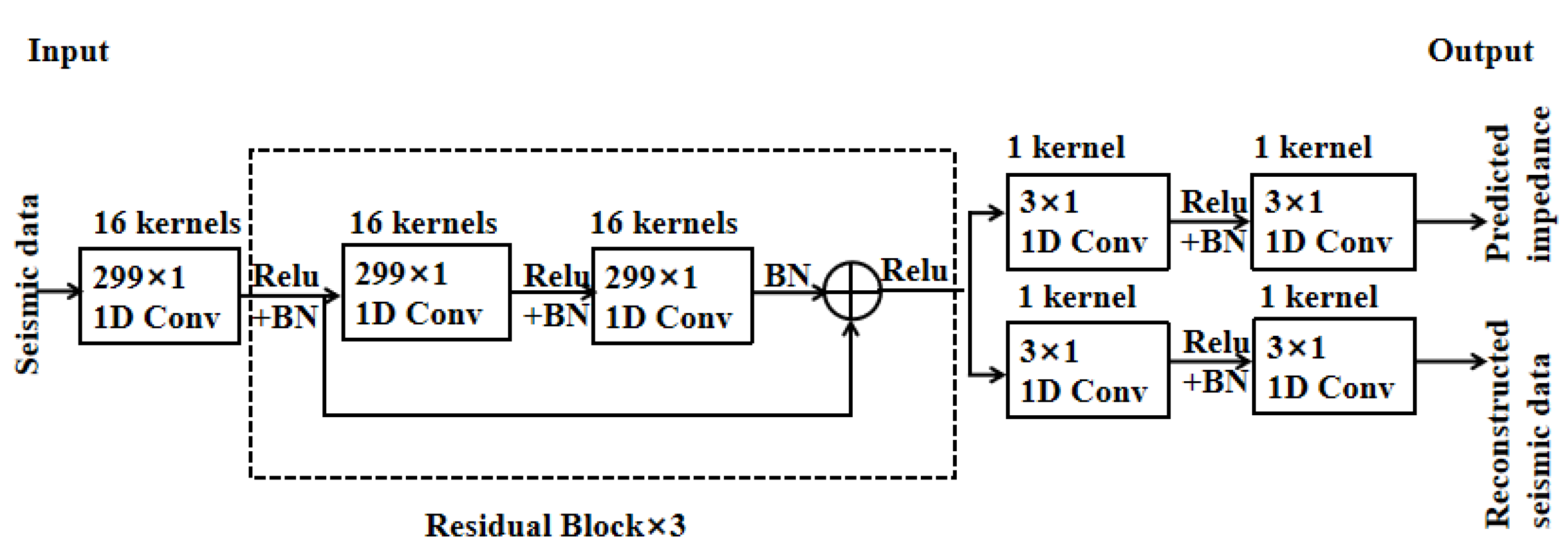
The single-task network used in this paper is a FCRN from Wu et al. [23], and the multi-task network is a hard parameter sharing network developed from the single-task FCRN. The multi-task network structure is shown in Figure 1. In order to better capture the low-frequency characteristics of seismic data, the first convolution layer of FCRN has 16 kernels of size 299 × 1. After the first convolution layer, three residual blocks are stacked, and each residual block is composed of two convolution layers. The first layer and the second layer, respectively, have 16 convolution kernels of size 299 × 1 and 3 × 1. To enable the network to complete multi-task inversion, two output channels are set after the residual block. Each output channel contains two one-dimensional convolution layers, and each one-dimensional convolution layer has a kernel of 3 × 1. The convolution step size is 1, and zero-padding is used to all convolution layers to ensure the same input and output sizes. Rectified linear unit (ReLU) and batch normalization (BN) are introduced into the network to accelerate network training and convergence.

2.2. Multi-Task Loss Function Based on Homoscedastic Uncertainty

The performance of hard parameter sharing is highly dependent on the loss weight of each task, and simply performing a weighted linear sum of the loss for each individual task is usually undertaken to carry out training. Manual tuning of the weights is often troublesome. Thus, a method based on homoscedastic uncertainty of the Bayesian model is used to balance the weights of the loss function of multiple tasks.

In Bayesian modeling, there are two main types of uncertainty, i.e., epistemic and aleatoric uncertainty. In a model, the aleatoric uncertainty captures the randomness of the model prediction, which depends on the noise inherent in input observations, and the epistemic uncertainty captures what a model does not know due to lack of training data [37]. Aleatoric uncertainty can again be divided into two subcategories, heteroscedastic uncertainty and homoscedastic uncertainty. Heteroscedastic uncertainty depends on the inputs to the model, with some inputs potentially having more noisy outputs than others. Homoscedastic uncertainty can be described as task dependent, which stays constant for all input data and varies between different tasks [36]. In this paper, we derive a multi-task loss function based on maximizing the Gaussian likelihood with homoscedastic uncertainty. The derivation is as follows:

(1)

Given a dataset $X=\left\{x_1,\dots ,x_N\right\}$, $Y=\left\{y_1,\dots ,y_N\right\}$, we define $f^w\left(x^{*}\right)$ as the output of a neural network with weights $w$ on input $x^{*}$. For regression tasks, we define the likelihood as a Gaussian distribution that takes the model output as the mean:

$$p\left(y^{*}|f^w\left(x^{*}\right)\right)=N\left(f^w\left(x^{*}\right),{\sigma }^2\right)$$

(1)

where $\sigma$ is an observation noise scalar capturing how much noise is in the outputs. When $w$ and $x^{*}$ are determined, the establishment of a probabilistic model of observation is equivalent to the determination of epistemic uncertainty and heteroscedastic uncertainty. Only homoscedastic uncertainty is considered in this paper. Different tasks have different homoscedastic uncertainties.

(2)

In maximum likelihood inference, we want to maximize the logarithmic likelihood of the model, that is, to maximize the following equation:

$$log p\left(y^{*}|f^w\left(x^{*}\right)\right)\propto -\frac{1}{2{\sigma }^2}\left|\right|y^{*}-f^w{\left(x^{*}\right)\left|\right|}^2-log\sigma$$

(2)

(3)

Construct the maximum likelihood function for multi-task. There are two tasks in our model: impedance prediction and data reconstruction. We use $y_{pre}$and$y_{rec}$ to denote the outputs of the two tasks and assume that $y_{pre}$and $y_{rec}$ following a Gaussian distribution:

$$p\left(y_{pre},y_{rec}|f^w\left(x\right)\right)=p\left(y_{pre}|f^w\left(x\right)\right)p\left(y_{rec}|f^w\left(x\right)\right)=N\left(y_{pre},f^w\left(x\right),{\sigma }_{pre}^2\right)N\left(y_{rec},f^w\left(x\right),{\sigma }_{rec}^2\right)$$

(3)

(4)

To maximize the logarithmic likelihood function, that is, to minimize the negative logarithmic likelihood function, then the multi-task loss function is:

$$\begin{gathered} \mathrm{L}\left(w,{\sigma }_{pre},{\sigma }_{rec}\right)=-log p\left(y_{pre},y_{rec}|f^w\left(x\right)\right)\propto \frac{1}{2{\sigma }_{pre}^2}\left|\right|y_{pre}-f^w{\left(x\right)\left|\right|}^2+\frac{1}{2{\sigma }_{rec}^2}\left|\right|y_{rec}-f^w{\left(x\right)\left|\right|}^2+log{\sigma }_{pre}{\sigma }_{rec} \\ =\frac{1}{2{\sigma }_{pre}^2}{L}_{pre}\left(w\right)+\frac{1}{2{\sigma }_{rec}^2}{L}_{rec}\left(w\right)+log{\sigma }_{pre}{\sigma }_{rec } \end{gathered}$$

(4)

the process of minimizing the loss function is to learn the optimal weight of $L_{pre}\left(w\right)$ and $L_{rec}\left(w\right)$ automatically according to the data. As ${\sigma }_{pre}$ increases, the weight of task impedance prediction decreases. However, with too great an increase in noise, the data will be ignored, so the last term of the objective function $log{\sigma }_{pre}{\sigma }_{rec}$ is the noise term regularizer. When the loss function reaches its minimum, we can obtain the corresponding ${\sigma }_{pre}$ and ${\sigma }_{rec }$. We use $w_{pre}$and$w_{rec}$ to denote the weights of the two tasks; then, from Equation (4) we can obtain the optimal weight between the two tasks as:

$$w_{pre} :w_{rec}=\frac{1}{2{\sigma }_{pre}^2} : \frac{1}{2{\sigma }_{rec}^2}={\sigma }_{rec }^2: {\sigma }_{pre}^2$$

(5)

Further processing makes the two weights add to 1; then, the final optimal weight is:

$$w_{pre} :w_{rec}=\frac{{\sigma }_{rec }^2}{{\sigma }_{pre}^2+{\sigma }_{rec }^2} : \frac{{\sigma }_{pre}^2}{{\sigma }_{pre}^2+{\sigma }_{rec }^2}$$

(6)

3. Experiments

Two synthetic datasets and one field dataset were used in this study, which are denoted as the Marmousi2 model, the Overthrust model, and the Volve model, respectively. The three datasets were used to train the single-task network and the hard parameter sharing multi-task network respectively, and then the trained networks were used for impedance inversion.

3.1. Experiment on the Marmousi2 Model

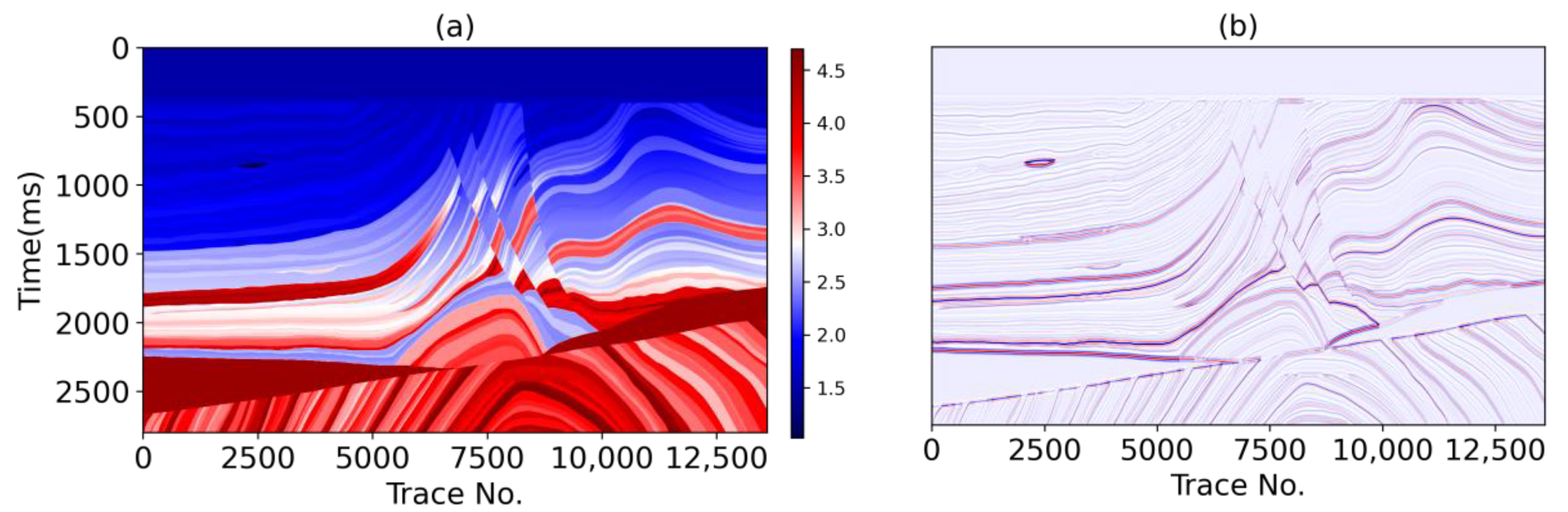
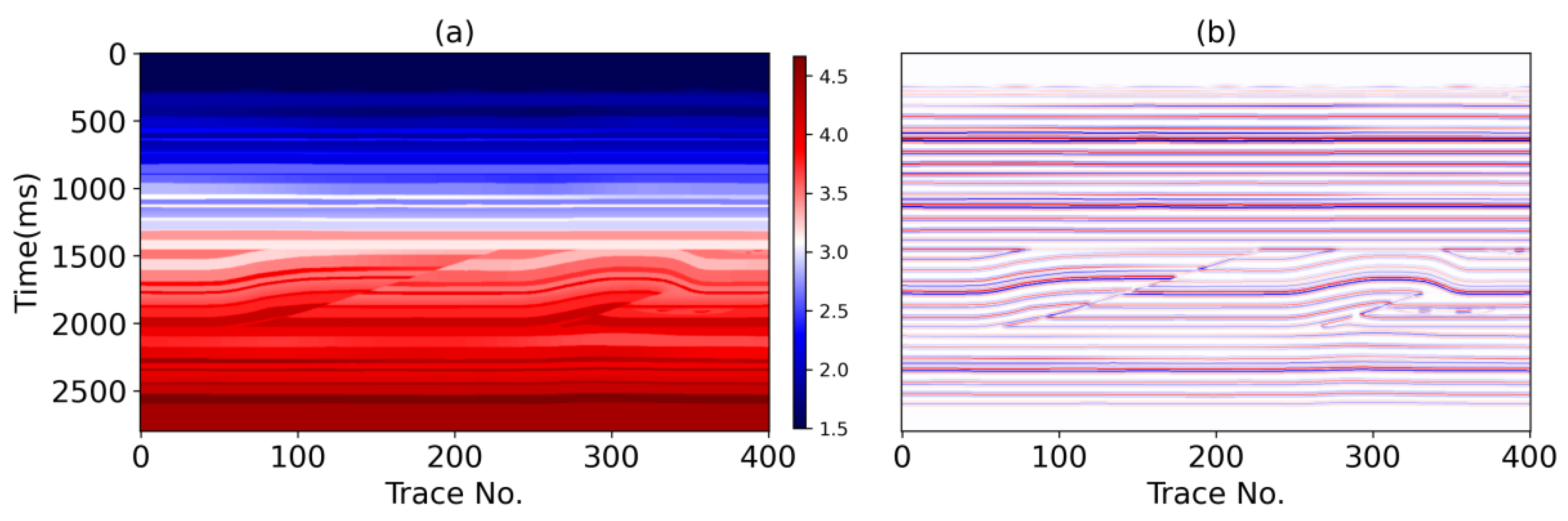
The impedance of the Marmousi2 model and its corresponding synthetic data are the same as in [23], and are shown in Figure 2. For this model, 101 traces were selected from the synthetic seismic data and impedance data as the training set through isometric sampling, and 1350 traces were randomly selected from the remaining 13,500 traces as the validation set and the whole 13,601 traces comprised the test set. The Adam optimization method was adopted in this paper. The weight decay rate was set to 1 × 10⁻⁷. The learning rate was set to 0.001. The number of epochs was set to 50, and the batch size was set to 10. The above hyperparameters and network structure were decided from an ablation study by adjusting the convergence of the training set and the validation set. The training of the network was implemented under the PyTorch framework, and a GPU was applied to accelerate the calculation.

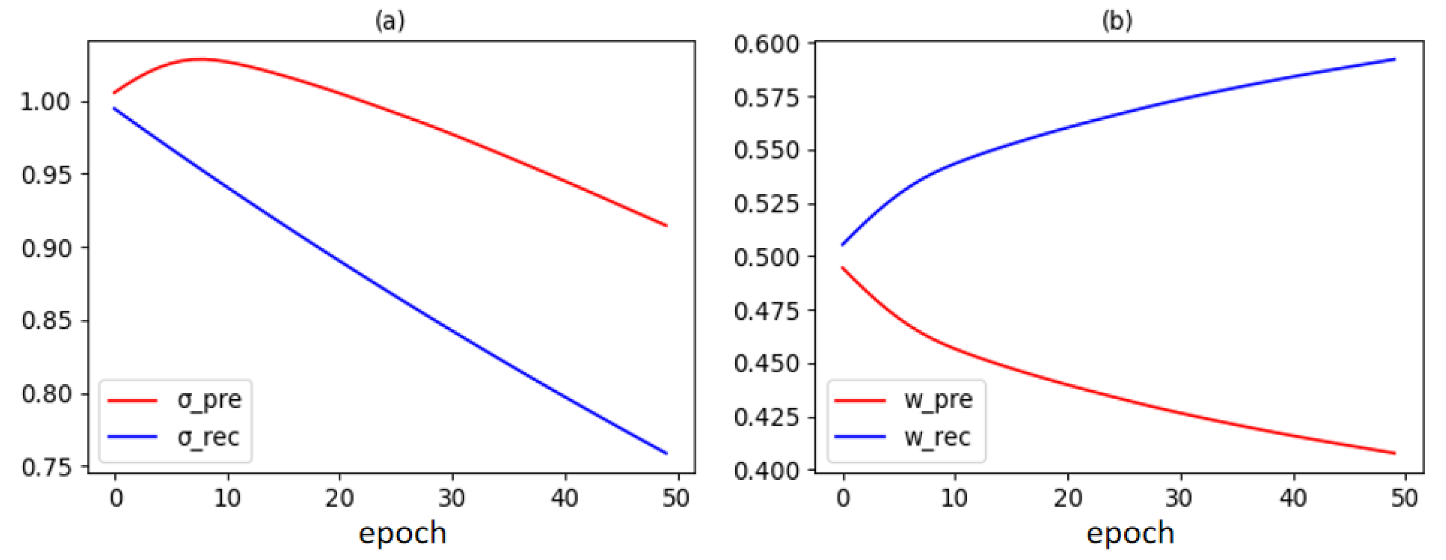
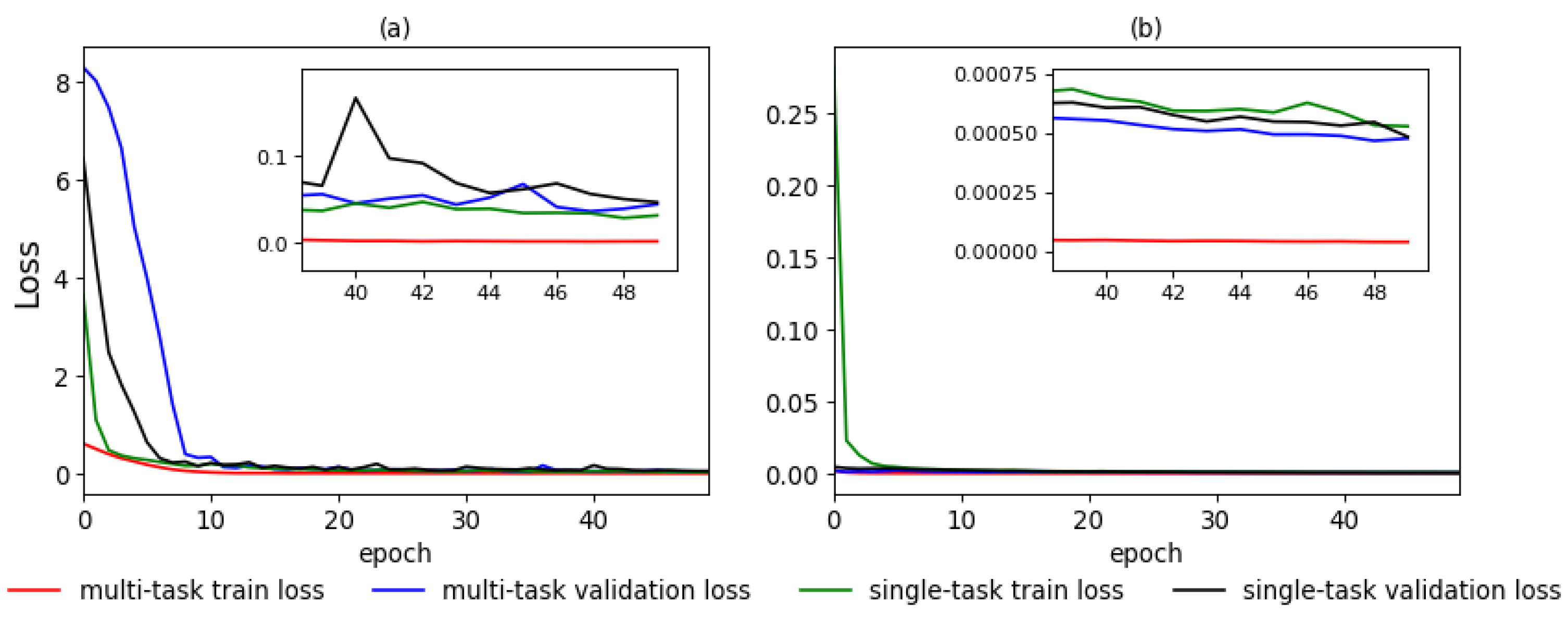
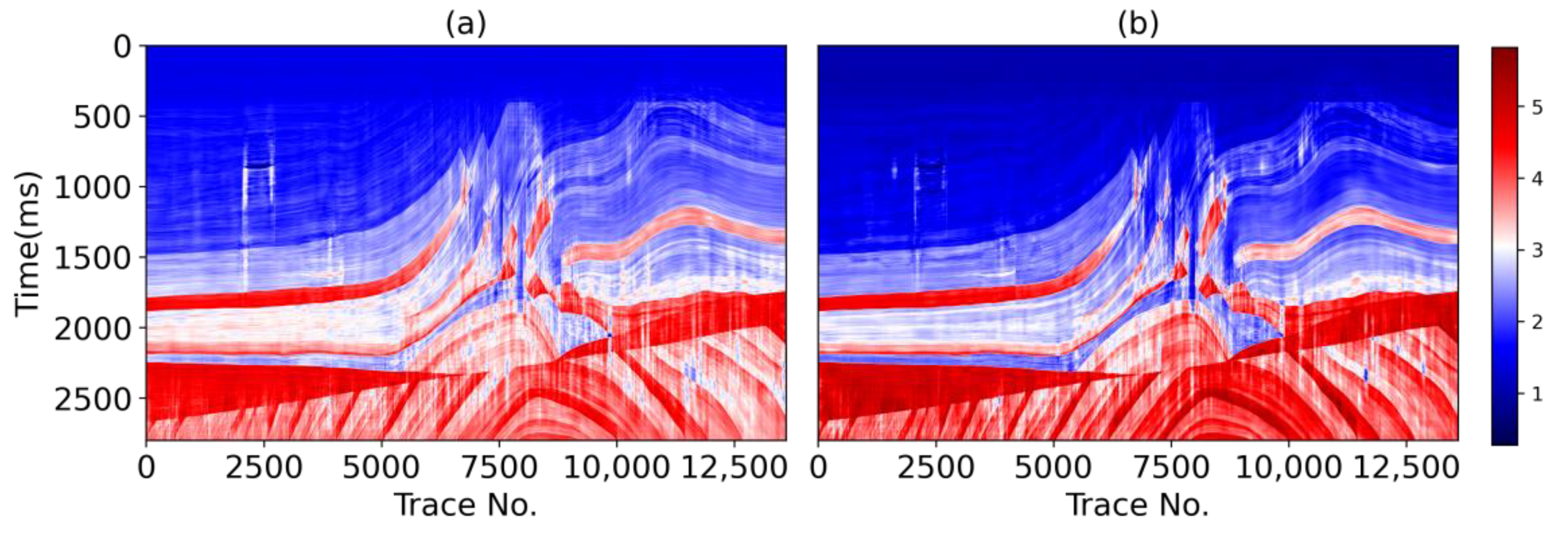
The validation Mean Squared Error (MSE) of the two tasks with different weights is shown in

Table 1. The validation MSEs of the two tasks with different weights on the Marmousi2 model.

Task Weights		MSE of Validation
$w_{pre}$(Impedance prediction)	$w_{rec}$(Data reconstruction)	Impedance prediction	Data reconstruction
0	1	/	0.00080
0.1	0.9	0.0411	0.00028
0.2	0.8	0.0412	0.00040
0.3	0.7	0.0407	0.00045
0.4	0.6	0.0397	0.00056
0.5	0.5	0.0372	0.00065
0.6	0.4	0.0374	0.00066
0.7	0.3	0.0397	0.00060
0.8	0.2	0.0385	0.00072
0.9	0.1	0.0375	0.00077
1	0	0.0446	/

. The training/validation procedure was executed five times and the average results were output for comparison. The performance of the model for a single task is shown in the first and last rows. When the validation loss is minimal during the 50 epochs, the corresponding ${\sigma }_{pre}$= 0.890 and ${\sigma }_{rec }$ = 0.759, then we can calculate that the optimal weight for impedance prediction and seismic data reconstruction is 0.421:0.579 by Equations (5) and (6). Figure 3 shows the variation at different epochs of ${\sigma }_{pre}$, ${\sigma }_{rec }$ and the corresponding $w_{pre}$, $w_{rec}$. Under this optimal weight, the validation MSE of the two task is 0.0365 and 0.00054. Compared with results in Table 1, it can be seen that the MSEs of the multi-task network of the two tasks under different weights are smaller than that of the single-task network, and the optimal weight determined by the proposed method makes the MSE smaller for both tasks, which proves the effectiveness of the method. The training and validation loss curves of different tasks under the optimal weight are shown in Figure 4. Figure 5 illustrates the profiles predicted by the single-task network (Figure 5a) and the hard parameter sharing multi-task network (Figure 5b) with the optimal weight for visual comparison. The MSEs of the profiles predicted by the single-task network and the hard parameter sharing multi-task network are 0.0478 and 0.0353, respectively, which proves the advantage of the hard parameter sharing multi-task network from a quantitative perspective.

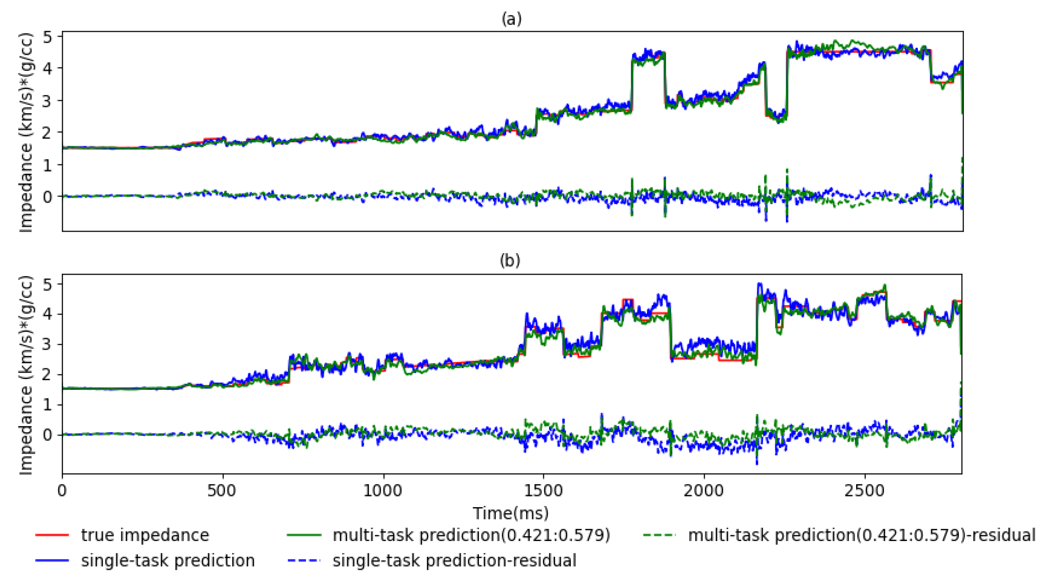
To further demonstrate the effectiveness of the proposed method, Figure 6 shows the results of impedance prediction for the 731st (Figure 6a) and 8991st (Figure 6b) trace data points. We can see that the impedance predicted by the hard parameter sharing multi-task network (green) matches the true impedance (red) better than that of the single-task network (blue). The blue and green dotted lines in Figure 6 represent residuals between the true impedance and the impedance predicted by the two networks.

Table 2. PCC between the traces’ predicted value and the ground truth of the Marmousi2 model.

Trace No.	Single-Task	Multi-Task (0.421:0.579)
731	0.9952	0.9956
8991	0.9805	0.9890

shows the Pearson Correlation Coefficient (PCC) between the predicted value and the truth. Under the optimal weights, the PCC between the predicted value and the ground truth of the 731st and 8991st traces of the multi-task network (third column) are both higher. We also tested the tolerance of the two networks to noise. We added six levels of Gaussian noise with a signal-to-noise ratio (SNR) of 0, 5, 15, 25, 35, and 45 dB to the test dataset. The MSEs between the prediction of different SNR data and the true impedance are presented in

Table 3. The MSEs between the prediction of different SNR data and the true impedance of the Marmousi2 model

SNR (dB)	Single-Task	Multi-Task (0.421:0.579)
0	1.1270	0.5948
5	0.2020	0.1260
15	0.0546	0.0379
25	0.0484	0.0355
35	0.0478	0.0353
45	0.0478	0.0353

, and shows that the accuracy of the multi-task network is higher than that of the single-task network under all six test datasets with different SNRs. This further proves the superiority of the method in this paper.

3.2. Experiment on the Overthrust Model

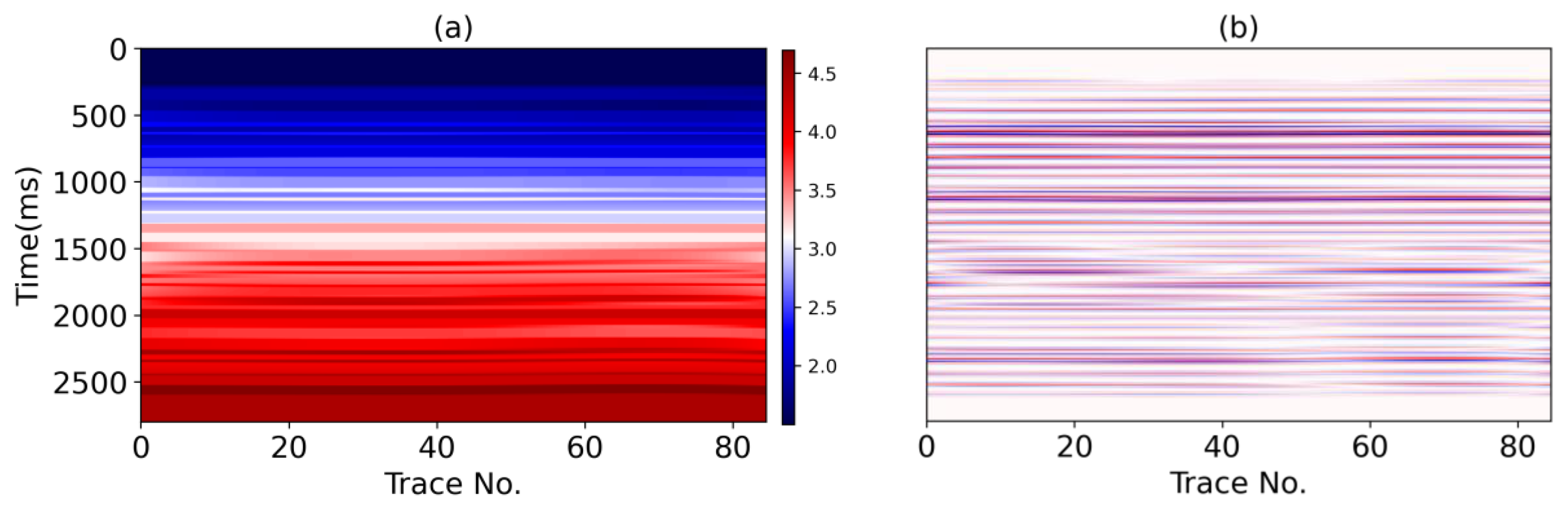
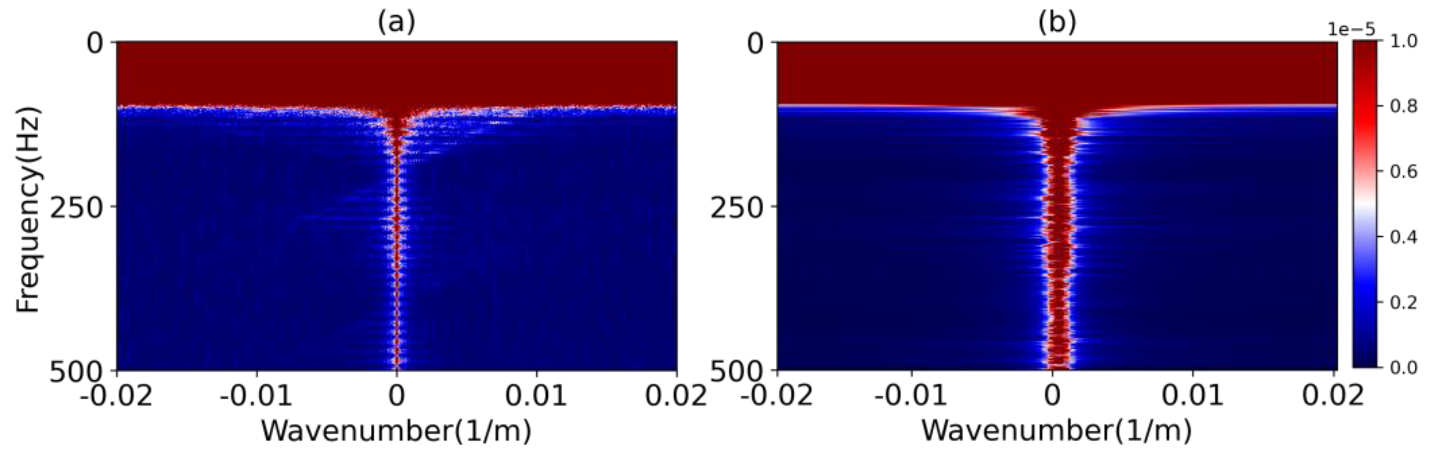
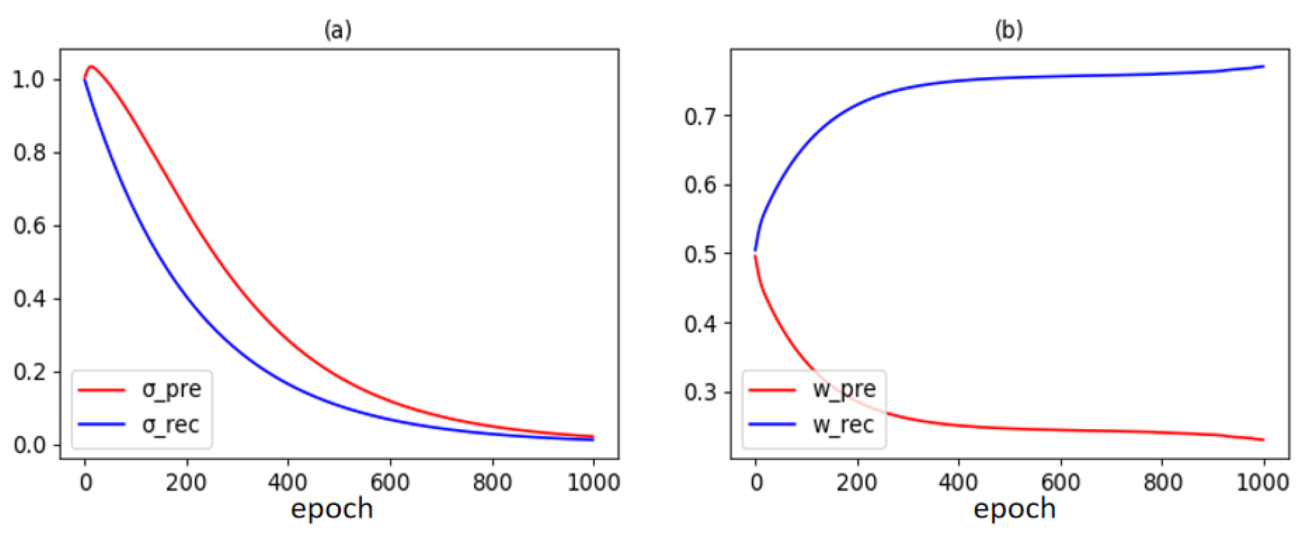
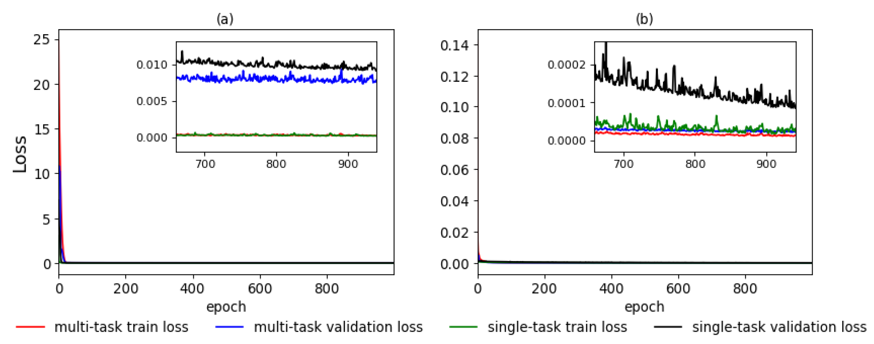
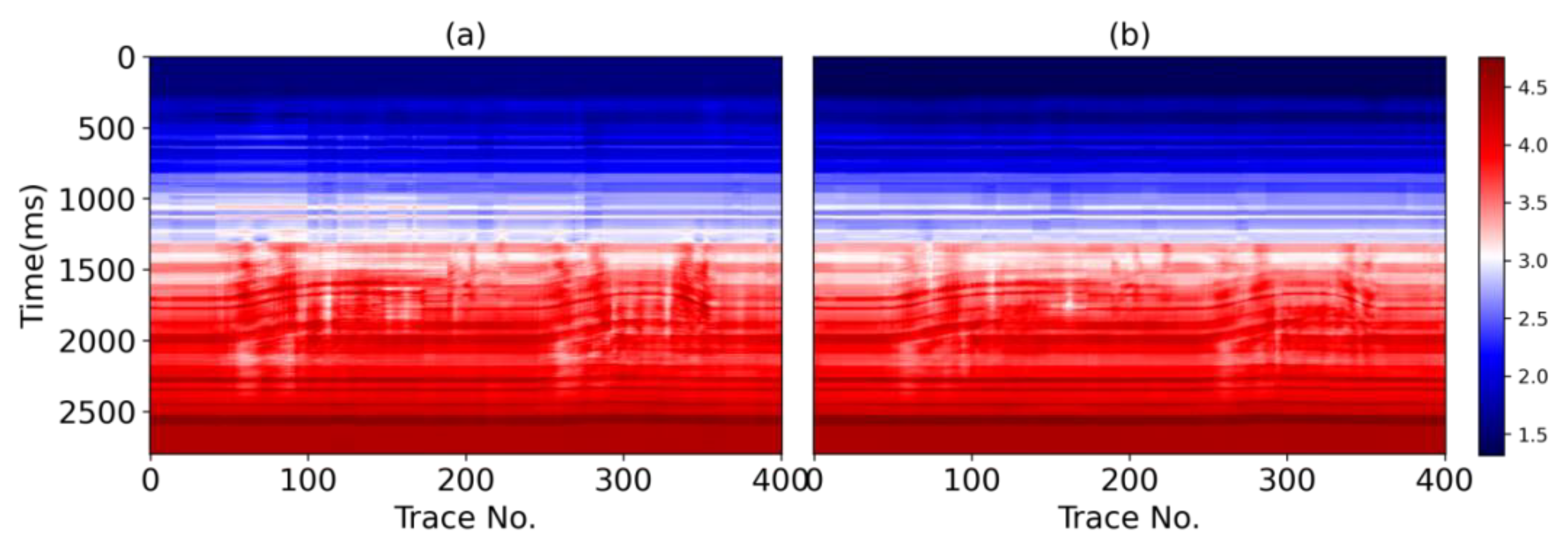
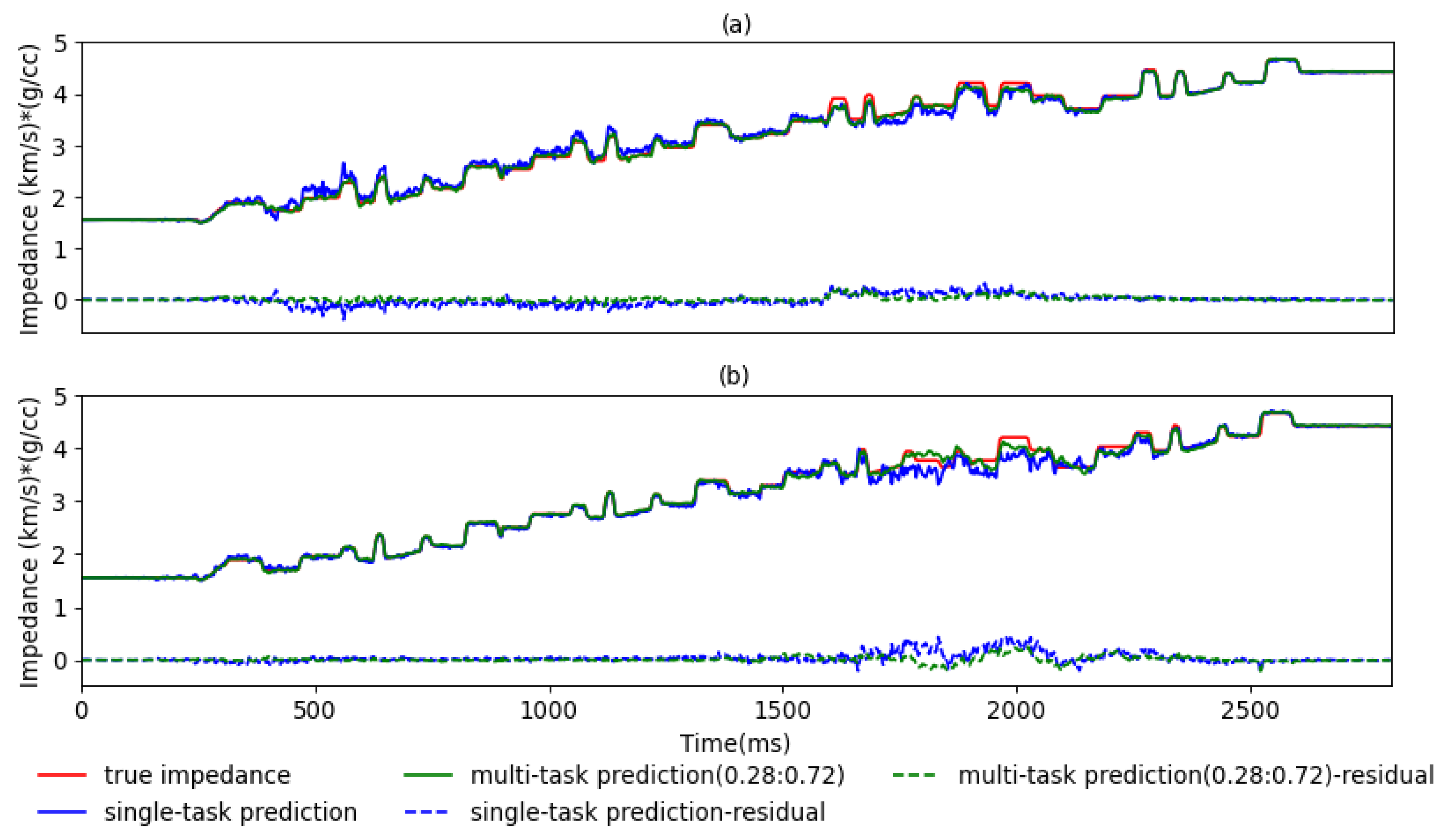
The impedance of the Overthrust model and its corresponding synthetic data are also that same as in [23] and are shown in Figure 7. For this model, five traces were selected as the training set from the synthetic seismic data and impedance data by isometric sampling, 39 traces were randomly selected from the remaining 392 traces as the validation set, and the whole 401 traces were the test set. Due to the small amount of sample data, there may be overfitting. Data enhancement methods are usually used to avoid overfitting. In contrast to the Marmousi2 model test, we used cubic spline interpolation to generate 20 new impedance and seismic data traces between every two selected traces in this model. Ultimately, we used 85 traces to train the network. The interpolation data are shown in Figure 8. The frequency-wavenumber spectra of the original and interpolated seismic data are shown in Figure 9 for comparison. The number of epochs was set to 1000 and the other hyperparameters and network structure were same as those of the Marmousi2 model. The validation MSEs of the two tasks with different weights are shown in

Table 4. The validation MSEs of the two tasks with different weights of the Overthrust model.

Task Weights		MSE of Validation
$w_{pre}$(Impedance prediction)	$w_{rec}$(Data reconstruction)	Impedance prediction	Data reconstruction
0	1	/	0.00005
0.1	0.9	0.0081	0.00002
0.2	0.8	0.0088	0.00003
0.3	0.7	0.0085	0.00001
0.4	0.6	0.0083	0.00002
0.5	0.5	0.0111	0.00004
0.6	0.4	0.0084	0.00003
0.7	0.3	0.0096	0.00001
0.8	0.2	0.0093	0.00006
0.9	0.1	0.0090	0.00007
1	0	0.0120	/

. The performance of the model for a single task is shown in the first and the last rows. When the validation loss is minimal during the 1000 epochs, the corresponding ${\sigma }_{pre}$= 0.192 and ${\sigma }_{rec }$ = 0.120, then we can calculate that the optimal weight is 0.28: 0.72, and the MSE of the two tasks under this weight is 0.0079 and 0.00001. Figure 10 shows the variation with epochs of ${\sigma }_{pre}$,${\sigma }_{rec }$ and the corresponding $w_{pre}$,$w_{rec}$. It can be seen that the MSEs obtained by the multi-task network under different weights for both tasks are all smaller than that obtained by the single-task network, and the optimal weight minimizes the MSEs. The training and validation loss curves of different tasks under the optimal weight are shown in Figure 11. Figure 12 illustrates the profiles predicted by the single-task network (Figure 12a) and the hard parameter sharing multi-task network (Figure 12b) with the optimal weight. The MSEs of the predicted profiles are 0.0119 and 0.0063, respectively, which also shows that the hard parameter sharing multi-task network outperforms the single-task network. Similarly, we chose two traces to further demonstrate the performance of the proposed method. Figure 13 shows the predicted results of impedance prediction for the 99th (Figure 13a) and 316th (Figure 13b) traces, and their corresponding PCC between the predicted value and the ground truth are shown in

Table 5. PCC between the traces’ predicted value and the ground truth of the Overthrust model.

Trace No.	Single-Task	Multi-Task (0.28:0.72)
99	0.9964	0.9993
316	0.9960	0.9990

. It is clear that the impedance predicted by the hard parameter sharing multi-task network (green) matches the true impedance (red) better than that by the single-task network (blue). The blue and green dotted lines in Figure 13 represent residuals between the true impedance and the impedance predicted by the two networks. In addition, the MSEs between the prediction of different SNR data and the true impedance are presented in

Table 6. The MSEs between the prediction of different SNR data and the true impedance of the Overthrust model

SNR (dB)	Single-Task	Multi-Task (0.28:0.72)
0	0.1300	0.2163
5	0.0295	0.0199
15	0.0128	0.0068
25	0.0120	0.0063
35	0.0119	0.0063
45	0.0119	0.0063

. It shows that, with the exception of 0 dB noise, the accuracy of the multi-task network is higher than that of the single-task network under the other five testing data with different SNRs, which further proves the advantage of the proposed method.

3.3. Experiment on the Volve Model

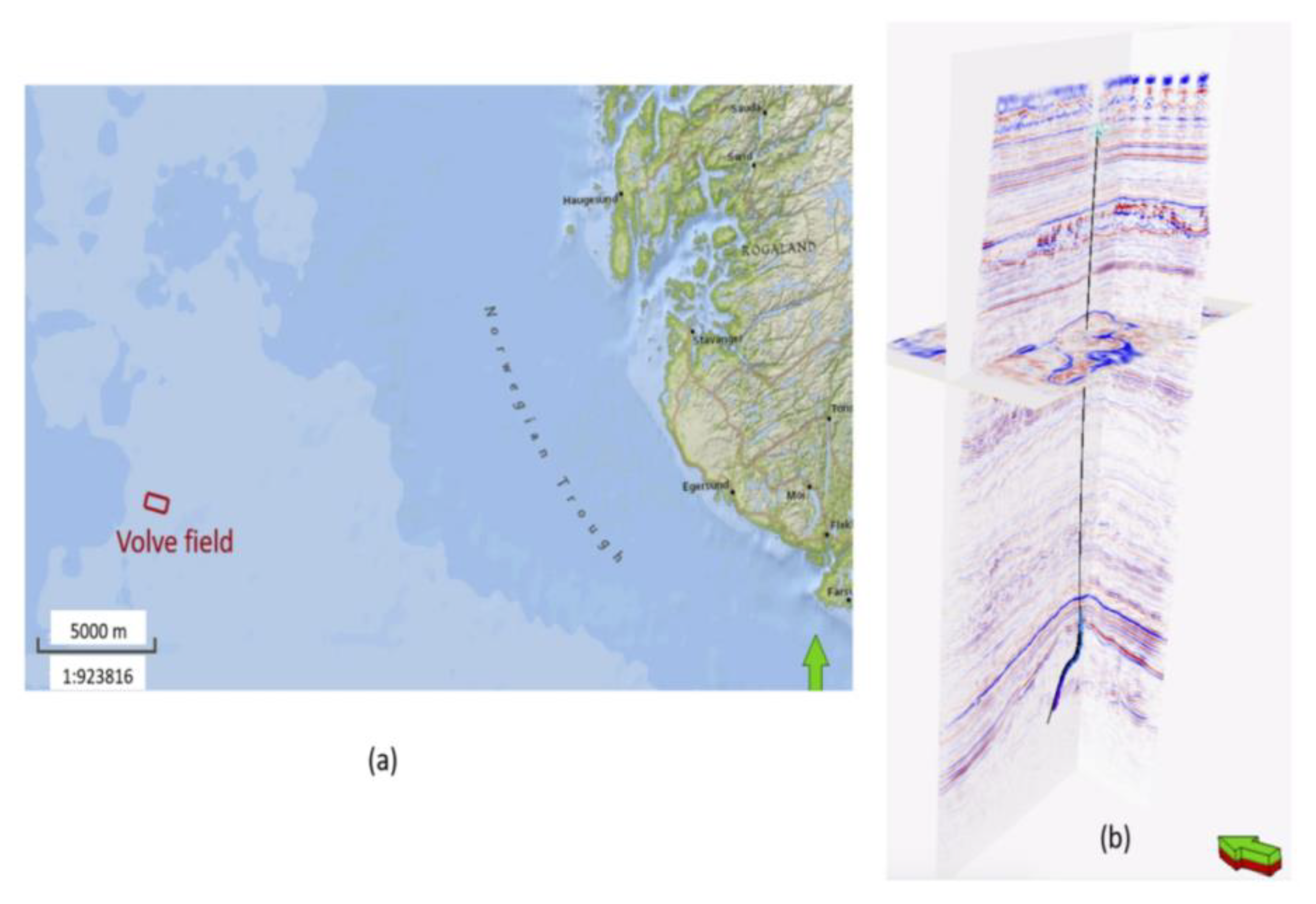
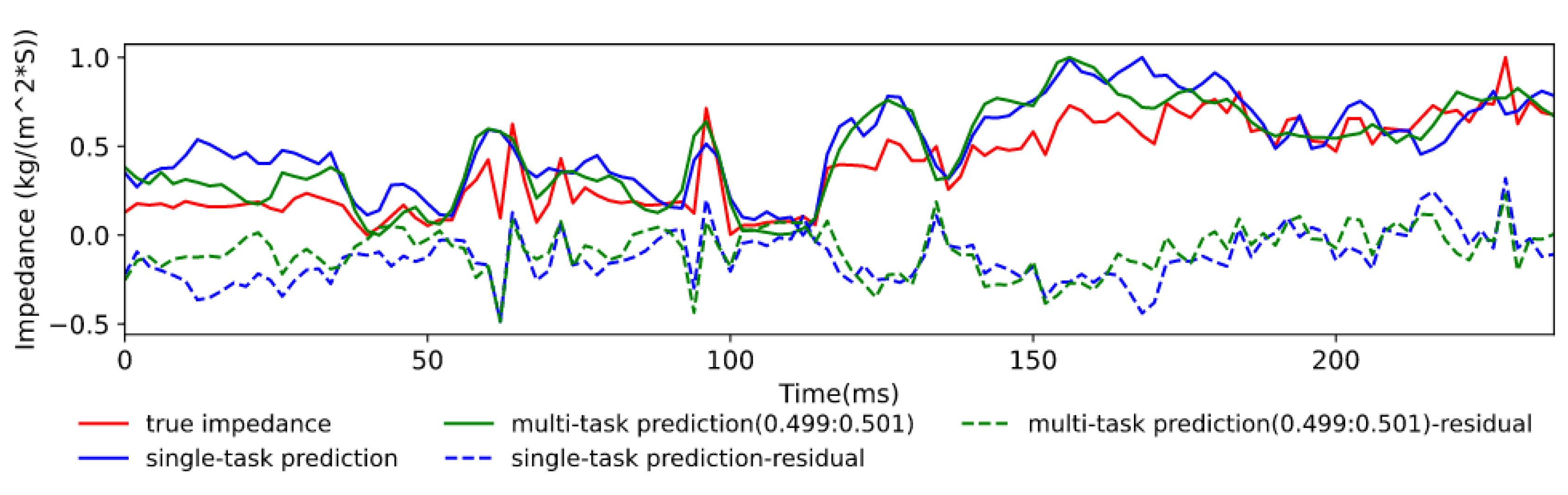
The field Volve data used in this paper are from the open-source code of Das et al. [19]. The Volve field shown in Figure 14a is located in offshore Norway and is a clastic reservoir. There are 1300 labeled traces in this dataset, which were generated using the data augmentation method in [19] based on the statistical characteristics of the well position log data shown in Figure 14b. We randomly selected 750 traces as the training set and the remaining 550 traces were set to be the validation set. We used the single true well log data to test the performance of the two networks. Unlike the previous two datasets, the kernel size was set as 80 to adapt the 160 time sampling points of the Volve model. The number of epochs was set to 500, and the other hyperparameters and network structure were set to be the same as in the former two models. Similarly, when the validation loss is minimal during the 500 epochs, the corresponding ${\sigma }_{pre}$= 0.829 and ${\sigma }_{rec }$ = 0.828, then we can calculate that the optimal weight for impedance prediction and seismic data reconstruction as 0.499:0.501. Figure 15 shows the predicted results of impedance prediction by the single-task model (blue) and the multi-task model (green) under the optimal weight. We can see that the impedance predicted by the multi-task model under the optimal weight matches the true impedance (red) better than the single-task model, especially in the time range between 40 and 50 ms. The blue and green dotted lines in Figure 15 represent residuals between the true impedance and the impedance predicted by the two networks. The MSE of the impedance predicted by the multi-task model under the approximate optimal weight is 0.0239, whereas the MSE predicted by the single-task model is 0.0352. In addition, the PCC between the ground truth and the values predicted by the multi-task model and the single-task model are 0.872 and 0.832, respectively. The above two metrics prove the superiority of the multi-task model under the optimal weight. It is worth noting that the test MSE and PCC in reference [19] are 0.0255 and 0.82, which is comparable with our single-task model, but is slightly inferior to our multi-task model. The Volve field data test shows that the proposed method in this paper improves the accuracy of impedance prediction on real seismic data.

4. Discussion

The proposed multi-task FCRN model was directly developed from the single-task FCRN of Wu et al. [23]. However, this is an open framework, enabling many other networks for seismic impedance prediction to also be explored. We believe seismic reconstruction is a task that is not limited to impedance inversion, and other deep learning tasks such as seismic fault interpretation can also benefit in similar way. Close inspection of Figure 3 and Figure 4 indicates that the almost flat total loss variation range corresponds to a relatively large range of $\left({\sigma }_{pre}, {\sigma }_{rec}\right)$. This means that there maybe not a single optimal weighting for all tasks, which was also an observation of Kendall et al. [36].

For the first two experiments, we attempted to add six levels of Gaussian noise, having an SNR of 0, 5, 15, 25, 35, and 45 dB, to the test set to test the tolerance of the two networks to noise. The test results of the Overthrust model show that the accuracy of the impedance prediction of the multi-task network is lower than that of the single-task network under the 0 dB noise. A possible reason for this is that when we add noise to the test dataset, we should train the model again to obtain a new optimal weight for the two tasks.

5. Conclusions

In this paper, we propose a multi-task network for both impedance inversion and seismic data reconstruction, and use a loss function based on the homoscedastic uncertainty of a Bayesian model to determine the optimal weight of the two tasks in the loss function. Test results from the Marmousi2, Overthrust, and Volve models show that: (1) the multi-task model has better generalization performance than the single-task model when the amount of labeled data is the same; and (2) the method proposed in this paper can be used to automatically determine the optimal weight of two tasks, and generates more accurate impedance than the single-task model. The proposed method can be extended to other multi-task learning approaches in a similar fashion.

In the future, we may apply the proposed method to high-dimensional seismic inversion, pre-stack inversion, and additional kinds of neural networks to verify its application value.

References

- Mustafa, A.; AlRegib, G. Joint learning for seismic inversion: An acoustic impedance estimation case study. In SEG Technical Program. Expanded Abstracts 2020; SEG Library: Houstin, TX, USA, 2020; pp. 1686–1690. [Google Scholar]
- Spadon, G.; Hong, S.; Brandoli, B.; Matwin, S.; Rodrigues, J.F., Jr.; Sun, J. Pay Attention to Evolution: Time Series Forecasting with Deep Graph-Evolution Learning. arXiv preprint 2020, arXiv:2008.12833. [Google Scholar] [CrossRef]
- Adler, A.; Araya-Polo, M.; Poggio, T. Deep learning for seismic inverse problems: Toward the acceleration of geophysical analysis workflows. IEEE Signal. Proc. Mag. 2021, 38, 89–119. [Google Scholar] [CrossRef]
- Hu, Y.; Zhang, Q.; Zhao, W.; Wang, H. TransQuake: A transformer-based deep learning approach for seismic P-wave detection. Earthq. Res. Adv. 2021, 1, 100004. [Google Scholar] [CrossRef]
- Wu, X.; Liang, L.; Shi, Y.; Fomel, S. FaultSeg3D: Using synthetic data sets to train an end-to-end convolutional neural network for 3D seismic fault segmentation. Geophysics 2019, 84, IM35–IM45. [Google Scholar] [CrossRef]
- Gao, K.; Huang, L.; Zheng, Y.; Lin, R.; Hu, H.; Cladohous, T. Automatic fault detection on seismic images using a multiscale attention convolutional neural network. Geophysics 2022, 87, N13–N29. [Google Scholar] [CrossRef]
- Wang, Z.; Li, B.; Liu, N.; Wu, B.; Zhu, X. Distilling knowledge from an ensemble of convolutional neural networks for seismic fault detection. IEEE Geosci. Remote Sens. Lett. 2020, 19. [Google Scholar] [CrossRef]
- Zhou, R.; Yao, X.; Wang, Y.; Hu, G.; Yu, F. Seismic fault detection with progressive transfer learning. Acta Geophys. 2021, 69, 2187–2203. [Google Scholar] [CrossRef]
- Jiang, J.; Ren, H.; Zhang, M. A Convolutional Autoencoder Method for Simultaneous Seismic Data Reconstruction and Denoising. IEEE Geosci. Remote Sens. Lett. 2021, 19. [Google Scholar] [CrossRef]
- Qiu, C.; Wu, B.; Liu, N.; Zhu, X.; Ren, H. Deep learning prior model for unsupervised seismic data random noise attenuation. IEEE Geosci. Remote Sens. Lett. 2021, 99, 1–5. [Google Scholar] [CrossRef]
- Wang, B.; Zhang, N.; Lu, W.; Wang, J. Deep-learning-based seismic data interpolation: A preliminary result. Geophysics 2019, 84, V11–V20. [Google Scholar] [CrossRef]
- He, T.; Wu, B.; Zhu, X. Seismic Data Consecutively Missing Trace Interpolation Based on Multistage Neural Network Training Process. IEEE Geosci. Remote Sens. Lett. 2021, 19, 1–5. [Google Scholar] [CrossRef]
- Li, X.; Wu, B.; Zhu, X.; Yang, H. Consecutively Missing Seismic Data Interpolation based on Coordinate Attention Unet. IEEE Geosci. Remote Sens. Lett. 2021, 19. [Google Scholar] [CrossRef]
- Yu, J.; Wu, B. Attention and Hybrid Loss Guided Deep Learning for Consecutively Missing Seismic Data Reconstruction. IEEE Trans. Geosci. Remote Sens. 2021, 60. [Google Scholar] [CrossRef]
- Greiner, T.A.L.; Lie, J.E.; Kolbjørnsen, O.; Evensen, A.K.; Nilsen, E.H.; Zhao, H.; Gelius, L.J. Unsupervised deep learning with higher-order total-variation regularization for multidimensional seismic data reconstruction. Geophysics 2021, 87, 1–62. [Google Scholar]
- Huang, W.L.; Gao, F.; Liao, J.P.; Chuai, X.Y. A deep learning network for estimation of seismic local slopes. Petroleum Sci. 2021, 18, 92–105. [Google Scholar] [CrossRef]
- Zhang, Z.; Lin, Y. Data-driven seismic waveform inversion: A study on the robustness and generalization. IEEE Trans. Geosci. Remote Sens. 2020, 58, 6900–6913. [Google Scholar] [CrossRef] [Green Version]
- Biswas, R.; Sen, M.K.; Das, V.; Mukerji, T. Prestack and poststack inversion using a physics-guided convolutional neural network. Interpretation 2019, 7, SE161–SE174. [Google Scholar] [CrossRef]
- Das, V.; Pollack, A.; Wollner, U.; Mukerji, T. Convolutional neural network for seismic impedance inversion. Geophysics 2019, 84, R869–R880. [Google Scholar] [CrossRef]
- Alfarraj, M.; AlRegib, G. Petrophysical property estimation from seismic data using recurrent neural networks. In Proceedings of the 2018 SEG International Exposition and Annual Meeting, Anaheim, CA, USA, 16 October 2018. [Google Scholar]
- Mustafa, A.; Alfarraj, M.; AlRegib, G. Estimation of acoustic impedance from seismic data using temporal convolutional network. In Proceedings of the SEG Technical Program, San Antonio, TX, USA, 15–20 September 2019; pp. 2554–2558. [Google Scholar]
- Li, H.; Lin, J.; Wu, B.; Gao, J.; Liu, N. Elastic Properties Estimation From Prestack Seismic Data Using GGCNNs and Application on Tight Sandstone Reservoir Characterization. IEEE Trans. Geosci. Remote Sens. 2021, 60. [Google Scholar] [CrossRef]
- Wu, B.; Meng, D.; Wang, L.; Liu, N.; Wang, Y. Seismic impedance inversion using fully convolutional residual network and transfer learning. IEEE Geosci. Remote Sens. Lett. 2020, 17, 2140–2144. [Google Scholar] [CrossRef]
- Wu, B.; Meng, D.; Zhao, H. Semi-supervised learning for seismic impedance inversion using generative adversarial networks. Remote Sens. 2021, 13, 909. [Google Scholar]
- Meng, D.; Wu, B.; Wang, Z.; Zhu, Z. Seismic Impedance Inversion Using Conditional Generative Adversarial Network. IEEE Geosci. Remote Sens. Lett. 2021, 19, 1–5. [Google Scholar] [CrossRef]
- Wang, Y.P.; Wang, Q.; Lu, W.; Ge, Q.; Yan, X. Seismic impedance inversion based on cycle-consistent generative adversarial network. Petroleum Sci. 2021. [Google Scholar] [CrossRef]
- Ghaderpour, E. Multichannel antileakage least-squares spectral analysis for seismic data regularization beyond aliasing. Acta Geophys. 2019, 67, 1349–1363. [Google Scholar] [CrossRef]
- Wu, X.; Yan, S.; Bi, Z.; Zhang, S.; Si, H. Deep learning for multidimensional seismic impedance inversion. Geophysics 2021, 86, R735–R745. [Google Scholar] [CrossRef]
- Ruder, S. An overview of multi-task learning in deep neural networks. arXiv preprint 2017, arXiv:1706.05098. [Google Scholar]
- Zhang, Y.; Yang, Q. A survey on multi-task learning. arXiv preprint 2017, arXiv:1707.08114. [Google Scholar] [CrossRef]
- Cao, D.; Ji, S.; Cui, R.; Liu, Q. Multi-task learning for digital rock segmentation and characteristic parameters computation. J. Petroleum Sci. Eng. 2022, 208, 109202. [Google Scholar] [CrossRef]
- Abu-Mostafa, Y.S. Learning from hints in neural networks. J. Complex. 1990, 6, 192–198. [Google Scholar] [CrossRef] [Green Version]
- Wang, Q.; Wang, Y.; Ao, Y.; Lu, W. Seismic inversion based on 2D-CNN and multi-task learning. In Proceedings of the 82nd EAGE Annual Conference & Exhibition, Amsterdam, Netherlands, Online, October 2021; pp. 1–5. [Google Scholar]
- Ku, B.; Min, J.; Ahn, J.K.; Lee, J.; Ko, H. Earthquake event classification using multitasking deep learning. IEEE Geosci. Remote Sens. Lett. 2020, 18, 1149–1153. [Google Scholar] [CrossRef]
- Duong, L.; Cohn, T.; Bird, S.; Cook, P. Low resource dependency parsing: Cross-lingual parameter sharing in a neural network parser. In Proceedings of the 53rd Annual Meeting of the Association for Computational Linguistics and the 7th International Joint Conference on Natural Language Processing, Beijing, China, 26–31 July 2015; Volume 2, pp. 845–850. [Google Scholar]
- Kendall, A.; Gal, Y.; Cipolla, R. Multi-task learning using uncertainty to weigh losses for scene geometry and semantics. In Proceedings of the IEEE Conference on Computer Vision and Pattern Recognition, Salt Lake City, UT, USA, 18–22 June 2018; pp. 7482–7491. [Google Scholar]
- Feng, R.; Grana, D.; Balling, N. Uncertainty quantification in fault detection using convolutional neural networks. Geophysics 2021, 86, M41–M48. [Google Scholar] [CrossRef]
Figure 1.
Architecture of the multi-task FCRN.
Figure 2.
Marmousi2 model dataset: (a) impedance; (b) synthetic seismic data generated by 30 Hz 0° phase Ricker wavelet.
Figure 3.
The variation of (a) , and (b) , with epochs.
Figure 4.
The training and validation loss curves of the Marmousi2 model: (a) impedance; (b) data reconstruction.
Figure 5.
Profiles of the Marmousi2 model predicted by (a) the single-task network and (b) the hard parameter sharing multi-task network under the optimal weights.
Figure 6.
Impedance traces’ prediction of the Marmousi2 model by the two networks: (a) trace 731; (b) trace 8991.
Figure 7.
Overthrust model dataset: (a) impedance; (b) synthetic seismic data generated with 30 Hz 0° phase Ricker wavelet.
Figure 8.
Interpolated data of the Overthrust model. (a) impedance; (b) synthetic seismic data.
Figure 9.
The frequency-wavenumber spectra of the original (a) and interpolated seismic data (b).
Figure 10.
Figure 11.
The training and validation loss curves of the Overthrust model: (a) impedance; (b) data reconstruction.
Figure 12.
Profiles of the Overthrust model predicted by (a) the single-task network and (b) the hard parameter sharing multi-task network under the optimal weight.
Figure 13.
Impedance traces prediction of the Overthrust model by the two networks: (a) trace 99; (b) trace 316.
Figure 14.
(a) The Volve field, as shown on a map, is located in the offshore North Sea area and (b) seismic data with a well trajectory from the Volve field (figure is from reference [19]).
Figure 15.
Impedance predicted for the well location of the Volve model by the two networks.