Least-Squares Reverse Time Migration in Imaging Domain Based on Global Space-Varying Deconvolution

Abstract

The classical least-squares migration (LSM) translates seismic imaging into a data-fitting optimization problem to obtain high-resolution images. However, the classical LSM is highly dependent on the precision of seismic wavelet and velocity models, and thus it suffers from an unstable convergence and excessive computational costs. In this paper, we propose a new LSM method in the imaging domain. It selects a spatial-varying point spread function to approximate the accurate Hessian operator and uses a high-dimensional spatial deconvolution algorithm to replace the common-used iterative inversion. To keep a balance between the inversion precision and the computational efficiency, this method is implemented based on the strategy of regional division, and the point spread function is computed using only one-time demigration/migration and inverted individually in each region. Numerical experiments reveal the differences in the spatial variation of point spread functions and highlight the importance to use a space-varying deconvolution algorithm. A 3D field case in Northwest China can demonstrate the effectiveness of this method on improving spatial resolution and providing better characterizations for small-scale fracture and cave units of carbonate reservoirs.

1. Introduction

High-resolution seismic imaging is a critical tool to acquire information on underground structures from observed seismic data [1,2]. Reverse time migration (RTM) has no assumption for the high-frequency approximation in traditional ray methods and shows good performance in lateral velocity varying media [3,4]. However, as the real data may have limited borehole diameter for observation, irregular observation systems, and limited wavelet frequency band, and thus images obtained from RTM have limited resolution and poor amplitude fidelity, providing inaccurate estimates of underground reflectivity [5].

By using the reverse Hessian operator on the conventional migration, the least-squares migration (LSM) allows for higher resolution, fewer migration artifacts, and better fidelity [6]. Since the Hessian matrix is too large in scale and the direct inversion process is not realistic, the LSM method is always recast as a data-driven linear optimization problem. Due to the good performance on improving resolution, it has been investigated in seismic imaging for acoustic-wave single component data [7,8,9,10,11,12,13,14,15,16,17,18] and elastic-wave multiple component data [19,20,21,22]. Besides, the elastic least-squares migration is extended to obtain multiparameter images, such as P- and S-wave velocity and density, to cope with the trade-off effects [23,24]. However, since this data-domain LSM has a high dependency on the accuracy of wavelet and velocity, most achievements for LSM are mainly obtained in theoretical experiments. Furthermore, in 3D data processing in practice, this data-domain LSM always suffers from unstable convergence and excessive computational cost, which make it quite difficult in practical applications.

In contrast, the imaging-domain LSM aims to find a reasonable approximation for the Hessian instead of performing the expensive iterative data-fitting process. The diagonal Hessian operator is commonly used to enhance the amplitude balance by considering the illumination for observation, providing similar results as the classical amplitude-preserving migration [25]. In horizontally layered media, the Green function for migration can be also used as a deconvolution operator, thus processing the results from migration [26,27]. An unsteady-phase filter can be estimated using the images from the front and rear iterations in data-domain LSM thus replacing the inversion in Hessian matrix to calibrate and filter the migration results [28,29,30,31]. Point spread function (PSF) from one scattering point is consistent with a row of elements in the Hessian matrix, which physically describes the impact of single-point-scattered energy on underground media, including local illumination characteristics of the observation geometry, the space variation in velocity model, and the band-limiting effect in seismic wavelet and received data [32,33]. These approximations for Hessian in imaging domain LSM can be also used as preconditioners for the data domain LSM, which, after multiple iterations, can more quickly approximate the real reflection coefficient [34,35,36,37].

However, as PSFs are of significant space-varying characters, it is rough to apply a space-invariant PSF from a single scattering point on the whole area. The novelty of our method is that it introduces a regional division strategy in the image-domain least-squares migration based on a global space-varying PSF. As a result, it can divide the global PSF into sub-blocks, use a high-dimensional space-varying deconvolution in each sub-block, and eventually perform the data reduction for all the sub-blocks. Since the continuity of velocity model and illumination is much better in local sub-blocks, the proposed method can provide high-resolution images and have computation efficiency.

2. Methodology and Principle

2.1. Basic Theory on LSM

The forward problem in the classical migration imaging can be expressed as:

$$d=Lm,$$

(1)

where, L is the linear operator in the linear Born simulation, which expresses the relation between underground reflectivity model m and seismic scattering data d. The migration images can be obtained by projecting the adjoint Born operator L^T into the seismic scattering data d:

$$I=L^{T}d.$$

(2)

The adjoint Borning operators $L^T$ can correctly reverse the propagation effects on the travel time and phase. However, due to problems such as limited observation apertures and limited data frequency band, the adjoint operator is not a good approximation for the inverse Born operators, which leads to unpreserved amplitude and low spatial resolution.

The LSM enables to provide high-fidelity images by minimizing the difference between synthetic and observed data, and the misfit function of the least-squares migration can be defined as,

$$\mathrm{C}\left(m\right)=\frac{1}{2}||Lm-d_{obs}||{}_2^2.$$

(3)

When the objective function reaches the minimum, the reflectivity model m satisfies the following equation:

$$I=\left(L^{T}L\right)=Hm.$$

(4)

In this equation, H is the Hessian operator, which is the second derivative of the misfit function (3). This equation is always named as the Newton normal equation, which establishes the basic principle for the LSM in the imaging domain and physically reveals that the migration image obtained by the conventional migration method is the Hessian-blurring version of the subsurface reflectivity model m. Thus, the seeking reflectivity model can be realized using the generalized inverse under the sense of the norm $L_2$.

$$m={\left(L^{T}L\right)}^{-1}I=H^{-1}I.$$

(5)

2.2. LSM in Imaging Domain

2.2.1. The Global Space-Varying Point Spread Function

According to the acoustic-wave equation, Hessian can be expressed in the frequency domain as:

$$H\left(x_1,x_2,\omega \right)=L{\left(x_1,\omega ;x_s,x_r\right)}^{T}L\left(x_2,\omega ;x_s,x_r\right),$$

(6)

where $x_s,x_r$ are the positions of shots and receivers, and L denotes the sensitivity kernel, satisfying

$$L\left(x,\omega ;x_s,x_r\right)=f\left(\omega \right)G\left(x,x_s,\omega \right)G\left(x,x_r,\omega \right),$$

(7)

where, f(ω) is a seismic wave, $G\left(x_1,x_s,\omega \right)$ is the Green function excited from the shot position $x_s$.

The PSF is commonly used as the approximation for Hessian, including a row of elements in the Hessian matrix $x_0$.

$$K\left(x_2,x_0,\omega \right)=L{\left(x_2,\omega ;x_s,x_r\right)}^T\left[L\left(x_0,\omega ;x_s,x_r\right)\delta \left(x-x_0\right)\right].$$

(8)

Here, $K\left(x_2,x_0,\omega \right)$ reflects the PSF of the perturbation at the point $x_0$.

Substitute Equation (8) into Equation (6), mark the point spread function at $x_i$ as ${\mathit{K}}_i$, and Hessian can be expressed as,

$$\mathit{H}={\left[\begin{array}{ccccc}{\mathit{K}}_1& \cdots & {\mathit{K}}_i& \cdots & {\mathit{K}}_m\end{array}\right]}^T.$$

(9)

Substitute the above equation into Equation (4) to obtain:

$${\mathit{I}}_i={\mathit{K}}_i\mathit{m}.$$

(10)

The reflectivity model can be obtained by

$$\mathit{m}=\frac{{\mathit{I}}_i}{\left({\mathit{K}}_i+\alpha \right)},$$

(11)

where α is the regularization parameter. The Equations (10) and (11) can be also expressed in the space domain as:

$${\mathit{I}}_i={\mathit{K}}_i*\mathit{m},$$

(12)

and:

$$\mathit{m}={\mathit{I}}_i\otimes {\mathit{K}}_i,$$

(13)

where, $*$ and $\otimes$ represent the operation of convolution and deconvolution, respectively. It reveals that, the migration image at $x_i$ is the superposition of the convolution of the global reflectivity model and the point spread function at $x_i$; on the contrary, the reflectivity model at $x_i$ can be computed within a high-dimensional deconvolution of the corresponding point spread functions.

2.2.2. Global Space-Varying Deconvolution

Equation (8) shows that the point spread function is exactly the image of the scattered wave radiated from the scattering point, which has a limited distribution in the space. Thus, the image-domain LSM can be based on the framework of the region division strategy, where the global point spread function can be divided into n blocks and the real impact of each point spread function is constrained within local neighborhoods $s_n$ to the scattering point $x_i$, $i=1,\dots ,s_n$,

$$K\left(x_n,x_i,\omega \right)=L{\left(x_n,\omega ;x_s,x_r\right)}^T\left[L\left(x_i,\omega ;x_s,x_r\right)\delta \left(x-x_i\right)\right].$$

(14)

Furthermore, within the neighborhood, the media velocity and illumination conditions are slowly varied, thus the PSFs for each position in $s_n$ can be assumed to be the same, and the reflectivity model for the neighborhood can be expressed as

$${\mathit{m}}_n={\displaystyle \sum }_{i\in s_n}{\mathit{I}}_i\otimes {\mathit{K}}_i={\mathit{I}}_n\otimes {\mathit{K}}_i.$$

(15)

Equation (15) means the regional reflectivity model for the neighborhood $s_n$ can be obtained by performing local deconvolution of the regional RTM image and the point spread function. The entire model can be obtained by stacking all the regional parts, and the global space-varying PSF can be computed using only one-time demigration and migration.

3. Analysis of Numerical Experiments

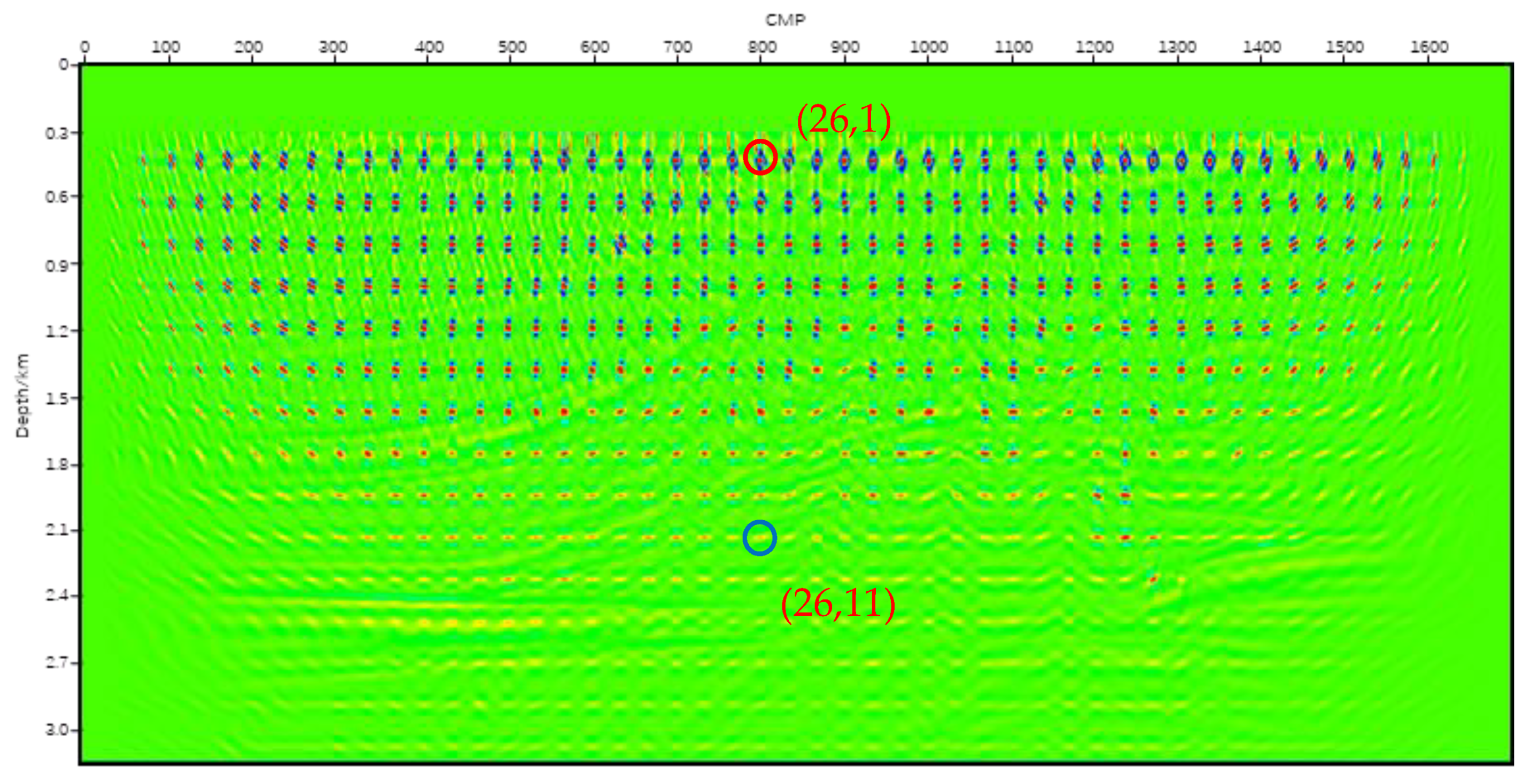
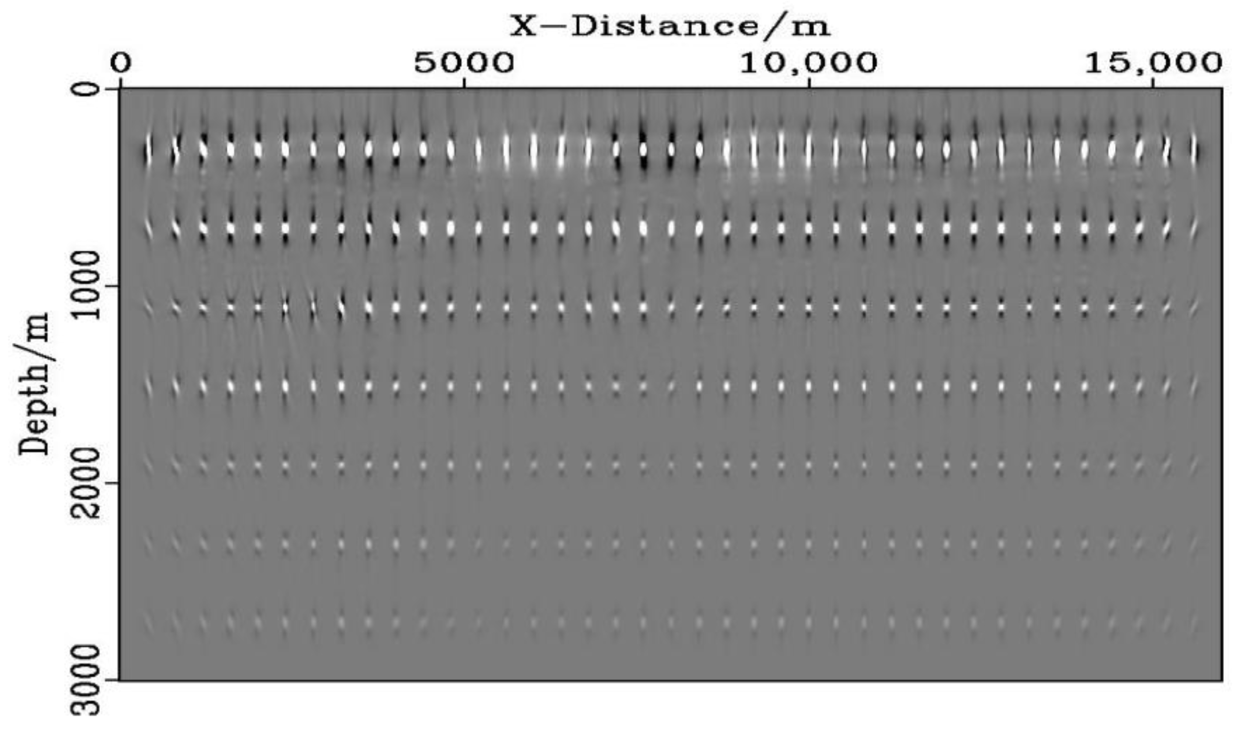
This section focuses on analyzing the physical characteristics of the point spread function. Figure 1 shows the global point spread function for the 2D Marmousi model. We can find the variations of observation illumination, wave propagation, and limited wavelet frequency-band at different positions. The propagation effect is mainly reflected in amplitude performance. Compared to the PSFs in the shallow model, those in the deep show much worse focusing with increasing attenuation radius. Since the RTM and PSF results are computed under the same observation system, the deconvolution can remove the influence of limited illumination angles in RTM results. Moreover, the seismic wavelets should match the one in RTM as they may have a great influence on point spread functions with respect to phase, amplitude, and attenuation radius.

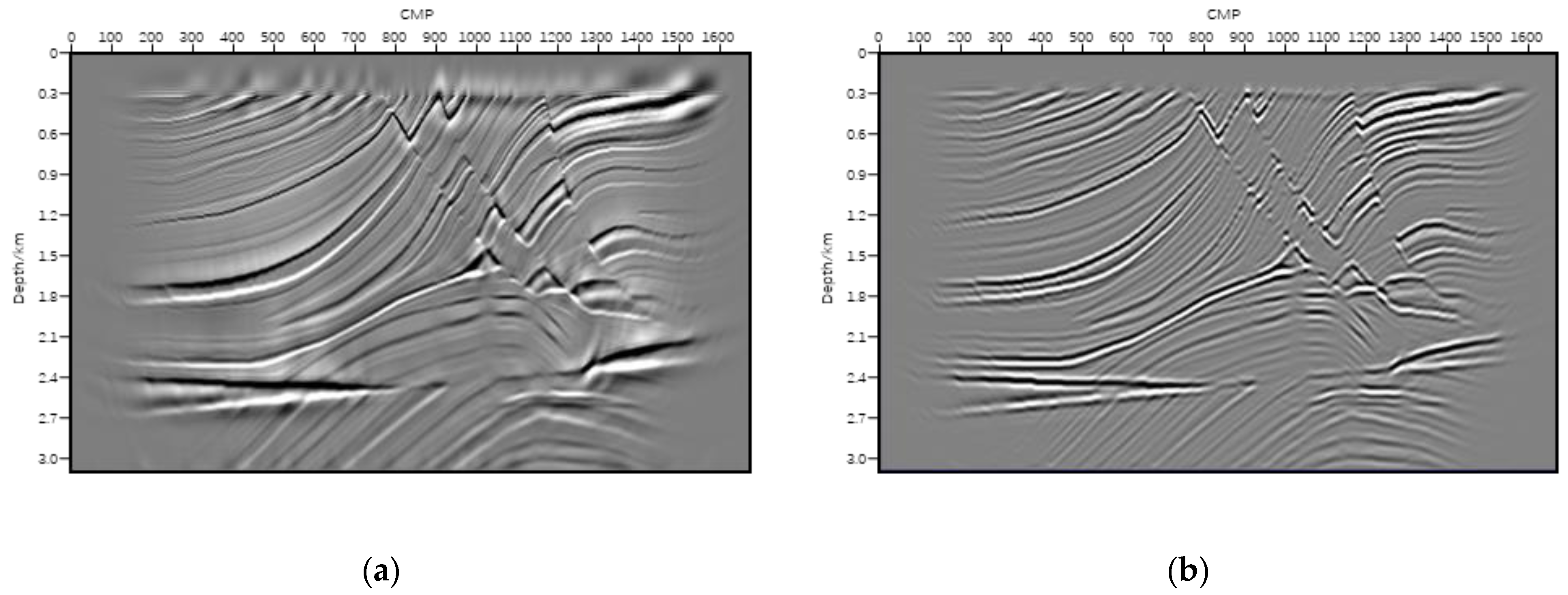
Figure 2 displays the inverted images using different point spread functions (red and blue circles in Figure 1). Even with the same wavelet, the images using the PSFs show significant variations in the space. The PSF at grid (26, 1) has wider illumination angles and better focusing than the one at grid (26, 11), and thus it can more accurately reflect the illumination characteristics of shallow structures in the model. As a consequence, the above PSF allows for better descriptions of the shallow structures but provides inaccuracy in the deep model. In contrast, due to limited illumination angle and wavefield propagation effect, the image obtained by the PSF at grid (26, 11) is much closer to an RTM result.

4. Numerical Experiment

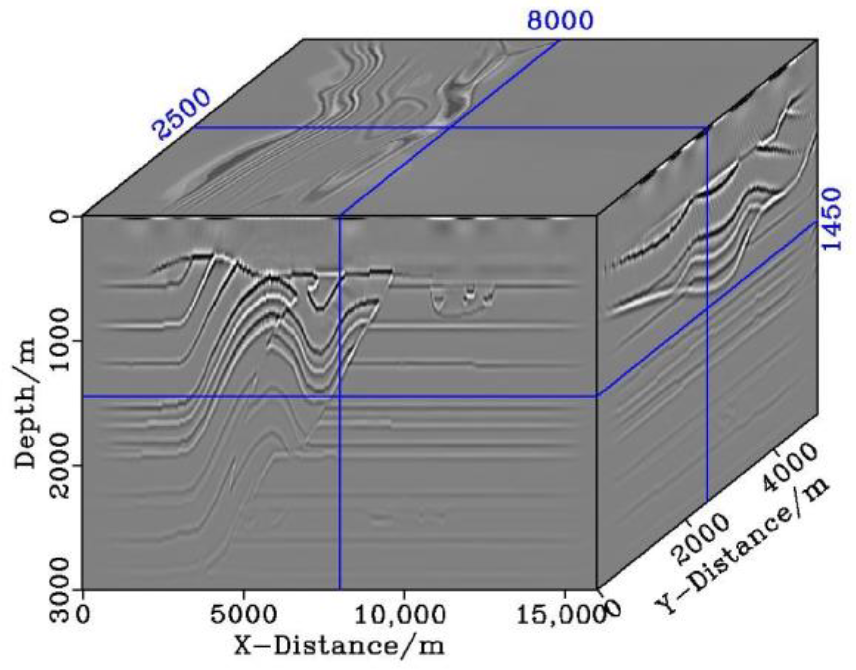
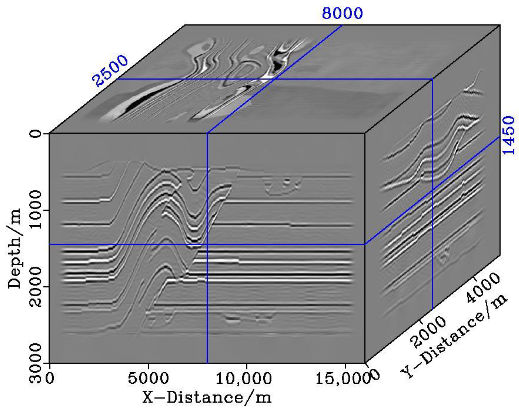
The method is tested on the 3D Overthrust model. The model is 16 km, 5 km, and 3 km in size, and the migration velocity is obtained by Gaussian smoothing with a window of 40 m. The Ricker wavelet with the main frequency of 30 Hz is used in this experiment. As shown in Figure 3, the RTM result has an insufficient spatial resolution, and the amplitude of the reflectors attenuates rapidly as the depth increases.

Then we compute the PSF using the same wavelet. Based on the migration velocity, the sampling interval (400 m, 400 m, 400 m) of the global PSF is set for the scattering model. To give intuitive insight into PSF, we present the X-Z tangent plane for point spread functions in Figure 4. As the geological structure and the illumination condition change, we can easily find that the difference of global PSFs in morphology is not negligible.

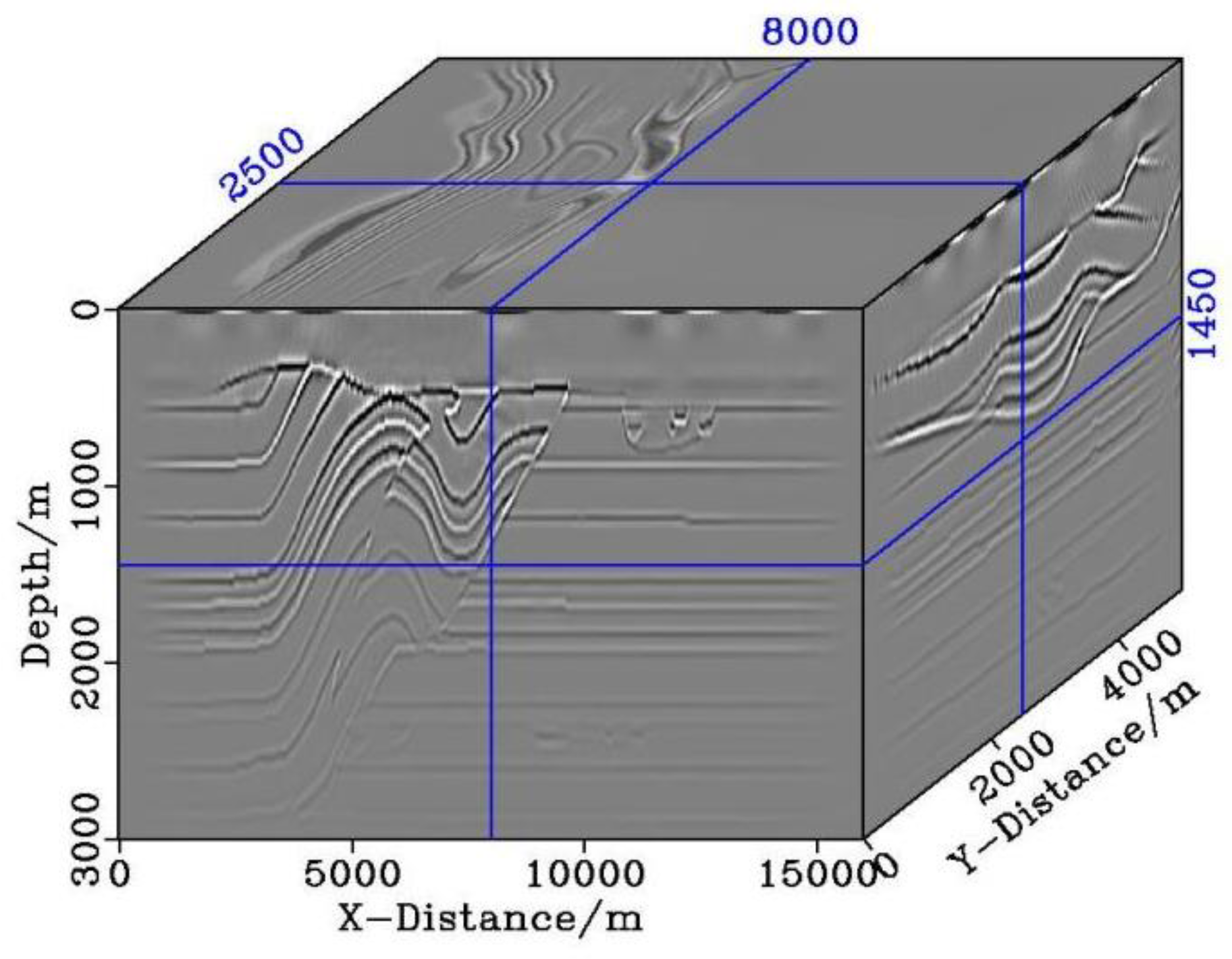
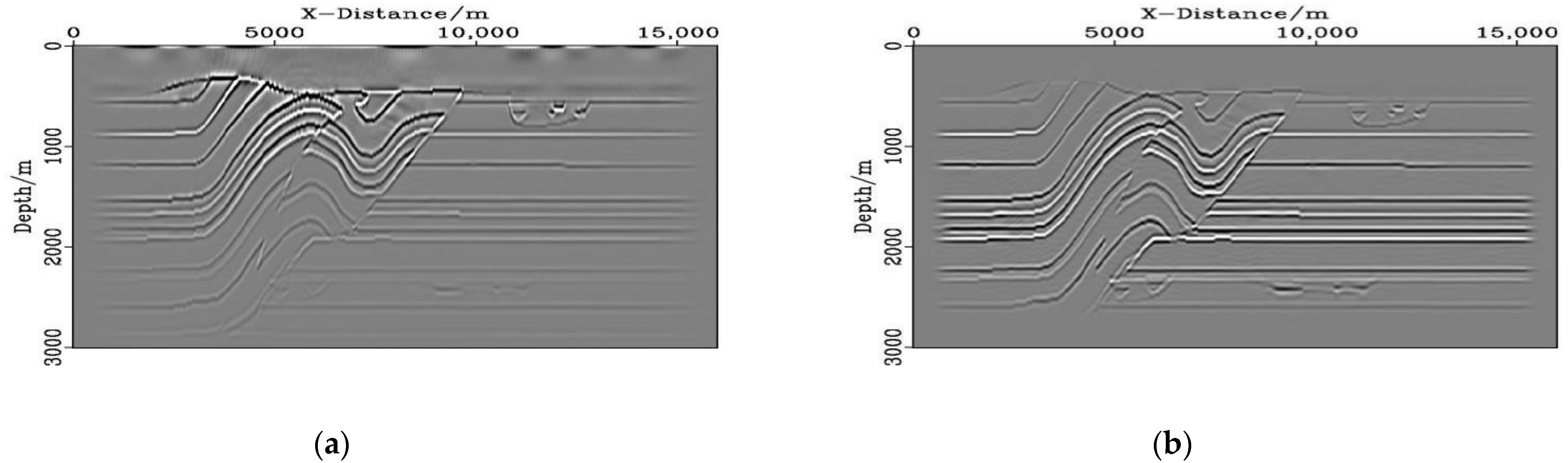
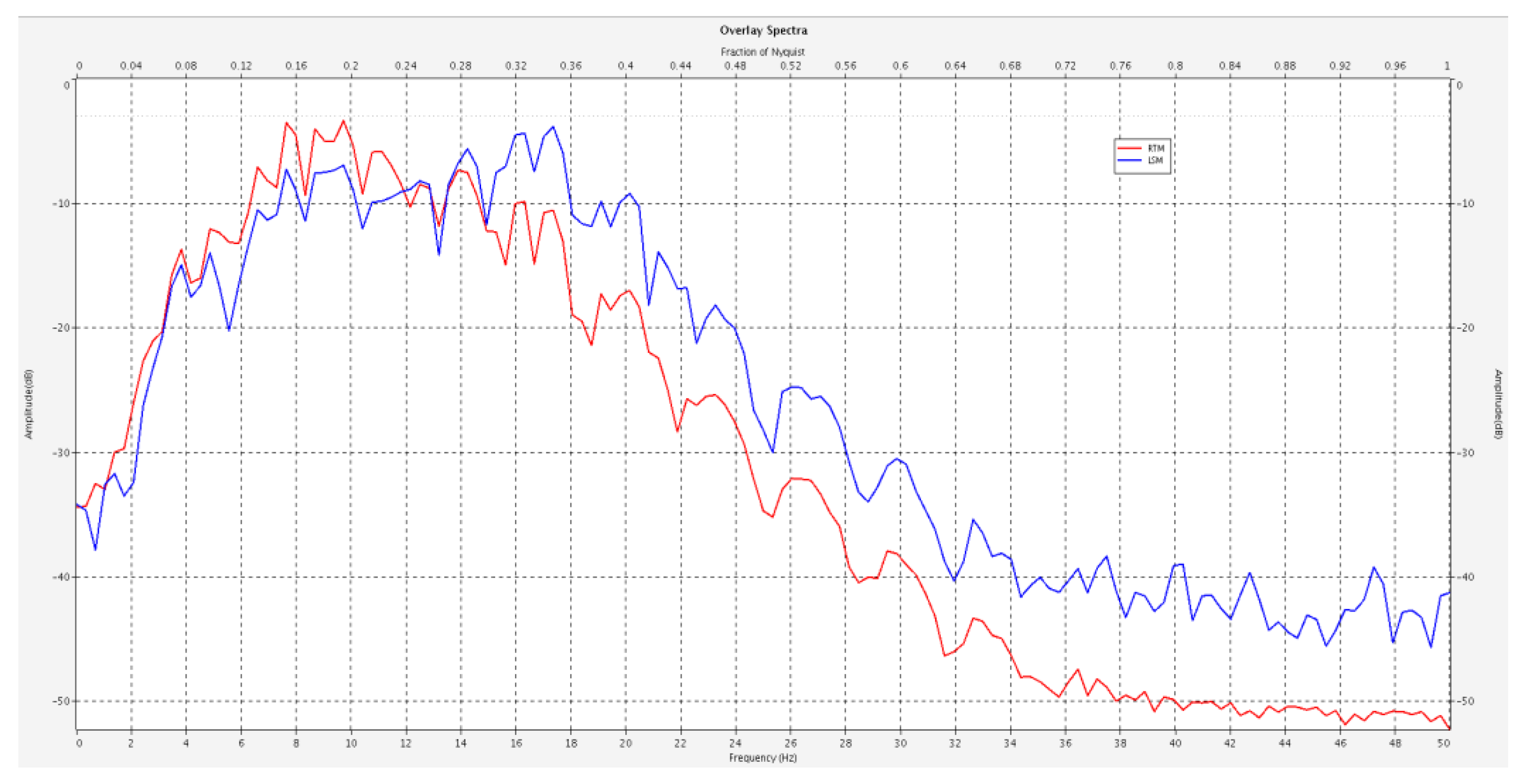
Figure 5 shows the results from the proposed imaging-domain LSM. Compared with the RTM results, the LSM results show higher resolution, fewer migration noise, more balanced amplitude in deep and better focusing on diffracted structures (as shown in Figure 6). To compare the spatial resolution between these results, we compute the vertical wavenumber spectrum of Figure 3 and Figure 5 for the whole model and present them in Figure 7. From the vertical wavenumber spectrum, we can find that the result from the LSM method has a broader frequency-band, especially for mid-high wave numbers. It means that the proposed LSM method can estimate the Hessian operator and remove those Hessian effects on the RTM results, which thus provides a more accurate reflectivity model.

5. Field Case

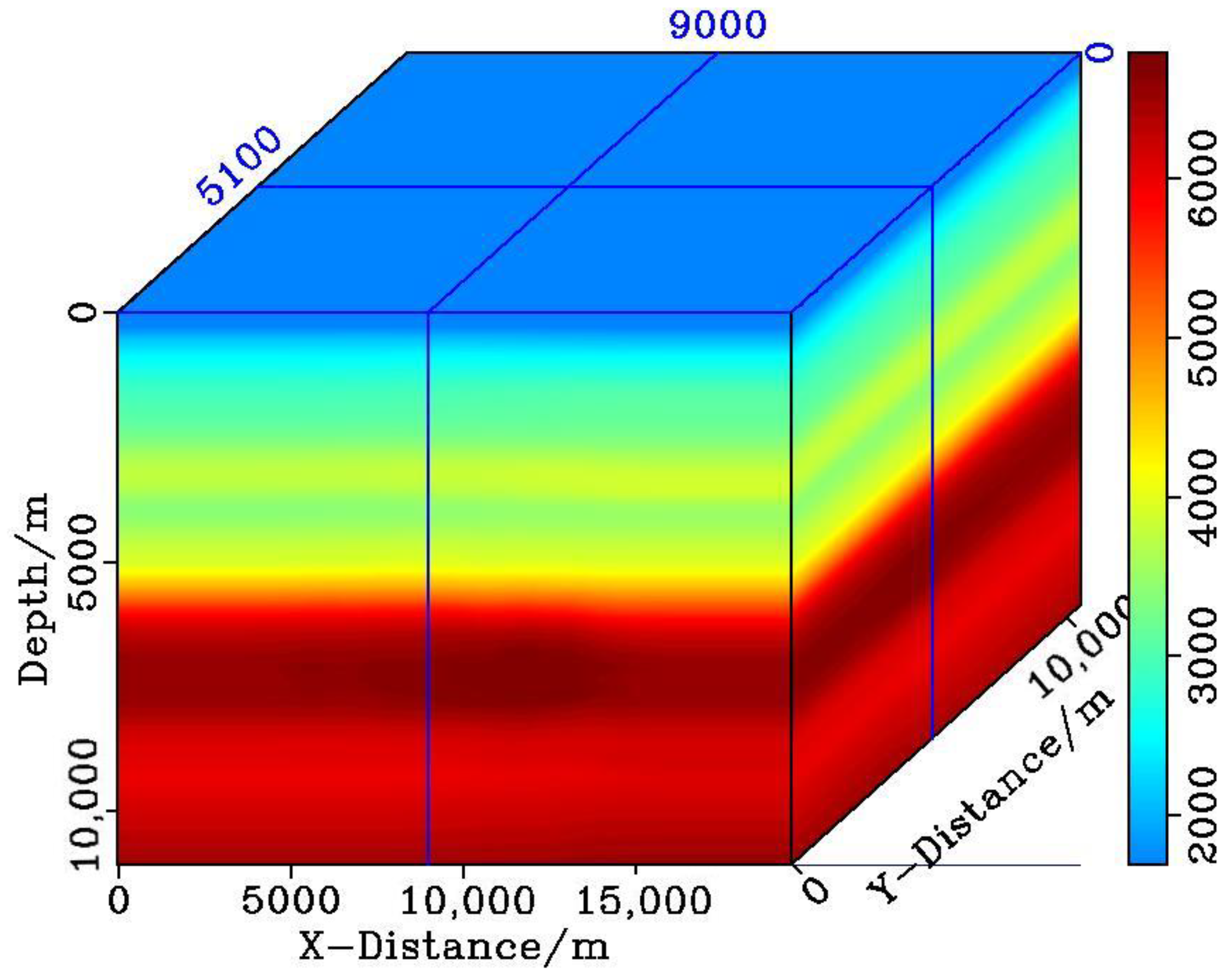
The target area is a part of the Tarim oil field in Northwest China, which is located in the middle of the North Tarim Uplift Belt to the east of the Halahatang depression. It has a large span, the target layer is deeply buried, the physical properties of the matrix are poor, and the type and scale of fracture caves are seriously affected by karst weathering. From the current development stage, the positioning accuracy of small and medium-sized karst cave cannot meet the requirements of resolution analysis of venting leakage around the well. In this work area, the geophone array recorded 33,000 shots at 5 m depth covering an area of 81 km². The main conundrum to be tackled in this work area is high-resolution imaging of Ordovician carbonate fracture-cavity reservoirs, with the depth ranging from 5.5 to 8 km. The migration velocity is built by a 3D travel time tomography as shown in Figure 8. The maximum cut-off frequency of the wavelet is 70 Hz.

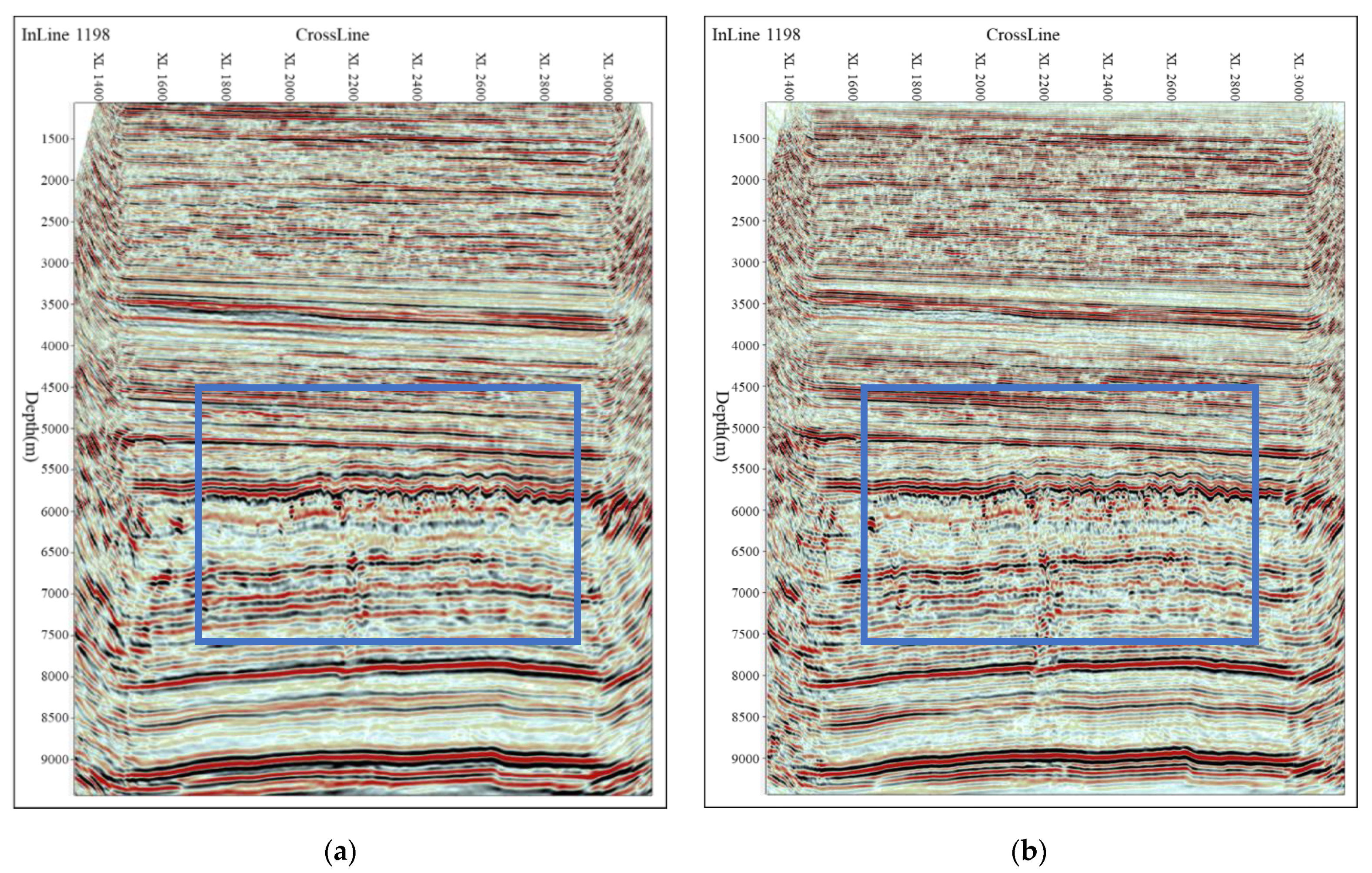
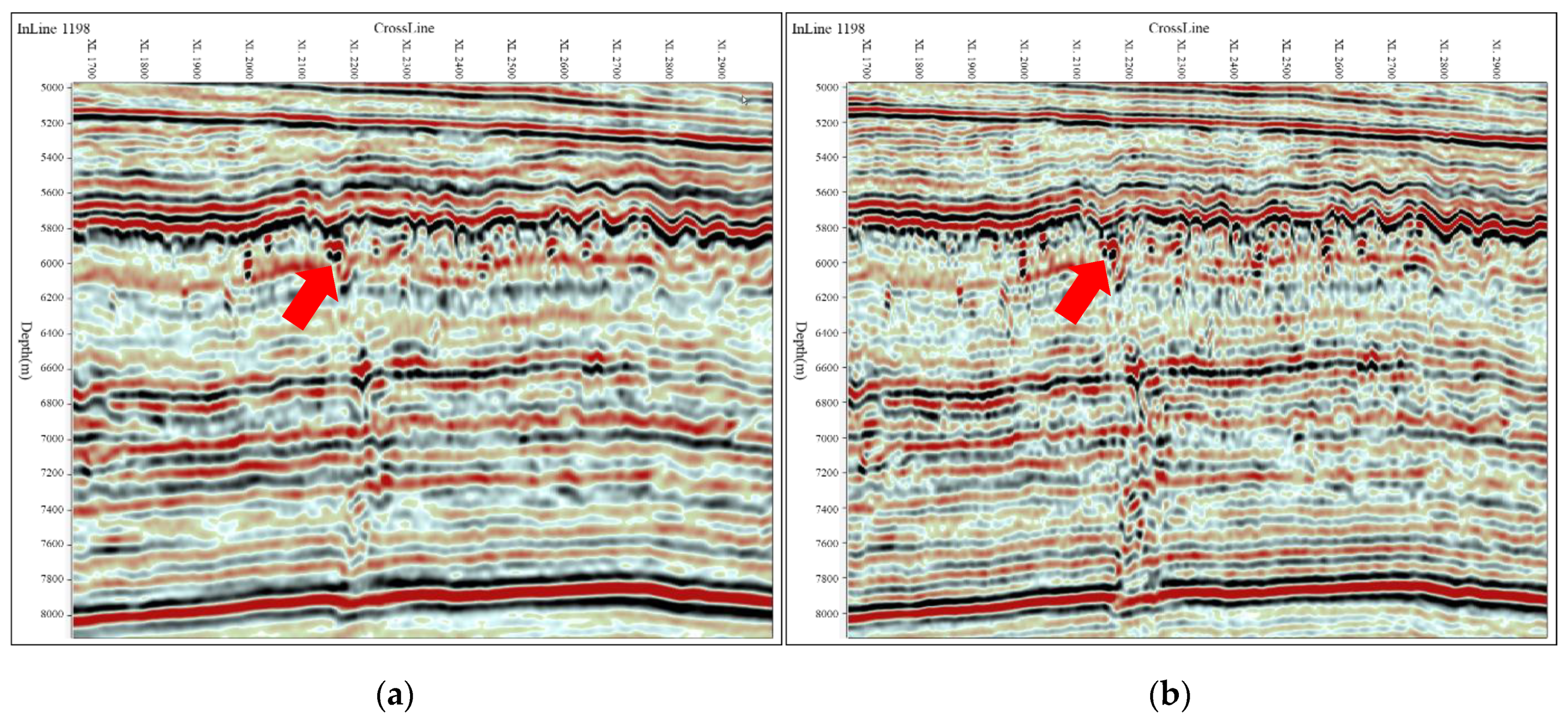
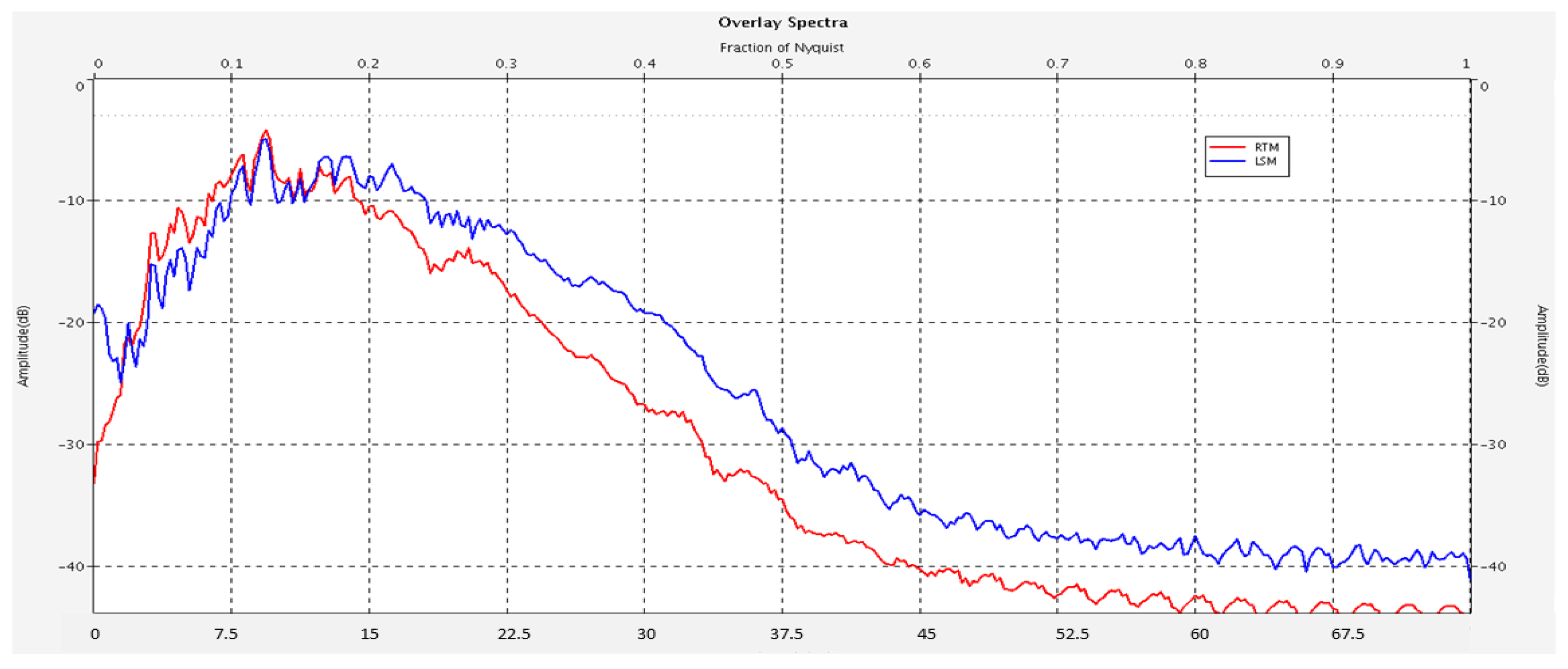
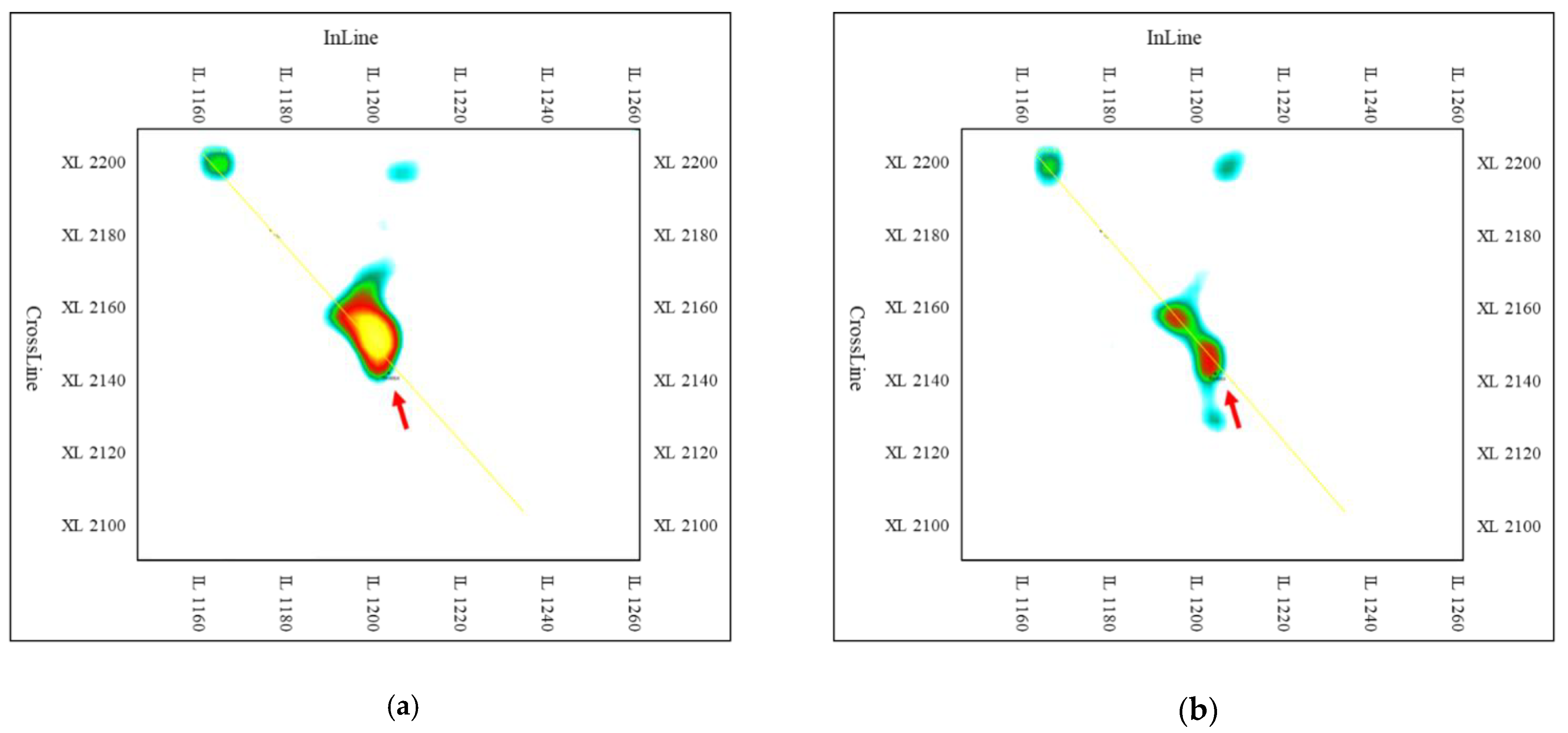
Figure 9 shows the results from RTM and LSM at the inline index of 200. Compared with the RTM results (Figure 9a), the LSM results (Figure 9b) provide higher spatial resolution, finer reflection events, more balanced amplitude, better focus ability, and more accurate fractured-cavity imaging. Figure 10 shows the zoomed region in Figure 9. We can find that the LSM result provides finer descriptions of fractured-cavity imaging and the boundaries between adjacent fractured-cavities, and the fractured-cavity bodies with small sizes in Ordovician carbonatite can be presented with higher resolution. Moreover, the deep fracture in the LSM result (Figure 10b) is better retrieved, which demonstrates that the proposed method is effective in fracture description. Figure 11 shows the vertical wave-number spectrum corresponding to the imaging results. The wave-number distribution of the LSM result is much broader, which lifts up at the low and mid-high sides of wave numbers. Besides, LSM can clearly provide information on cavities in the fracture zones, provide a high-quality scientific basis to analyze the development of fracture-controlled fractured-cavities and give guidance to the interpretation of reservoirs. To give an intuitive sight of the caves in Figure 10 denoted by red arrows, we compute the amplitude attributes from the RTM and LSM results and present a regional transverse section at the depth of these caves in Figure 12. We can find that the LSM results can distinguish the adjacent caves and provide better focusing, highlighting the proposed method can provide a high resolution in the horizontal direction and give a great help for reservoir interpretation and development. However, due to the limited observation aperture and shallow desert area, conventional RTM cannot provide correct images. The logging result located at the arrows in Figure 12 can also support the migration results, highlighting the effectiveness of the proposed method.

6. Conclusions

Utilization of the point spread function and the global space-varying high-dimension deconvolution algorithm effectively solves the demand of excessive computation in the iterative data-fitting process of classical least-squares migration and alleviates the high dependency on the accuracy of seismic wavelet and velocity model. Both the theoretical analysis and the model experiment demonstrate that the global space-varying point spread function can effectively approximate the Hessian and the high-dimensional spatial deconvolution algorithm can replace the deburring effects from the Hessian operator. The application on a field 3D data suggests that the method is effective in improving the imaging resolution, especially for caves and fractures, and provide higher-quality seismic images for ultra-deep fractured-cavity reservoirs.

References

- Moreno, W.; Galeano, I. Solution of high velocity anomalies imperceptible to seismic resolution, by means of synthetic models, Penobscot Field, Canada. Rud. Geološko-Naft. Zb. 2019, 34, 71–82. [Google Scholar] [CrossRef] [Green Version]
- Moreno, W.; Galeano, I. Identification of high velocity anomalies, imperceptible to seismic resolution, by integration of seismic attributes, in the Penobscot Field, Canada. Rud. Geološko-Naft. Zb. 2019, 34, 13–26. [Google Scholar] [CrossRef] [Green Version]
- Baysal, E.; Dan, D.K.; Sherwood, J.W.C. Reverse time migration. Geophysics 1983, 48, 1514–1524. [Google Scholar] [CrossRef] [Green Version]
- McMechan, G.A. Migration by extrapolation of time-dependent boundary values. Geophys. Prospect. 1983, 31, 413–420. [Google Scholar] [CrossRef]
- Nemeth, T.; Wu, C.; Schuster, G.T. Least-squares migration of incomplete reflection data. Geophysics 1999, 64, 208–221. [Google Scholar] [CrossRef]
- Schuster, G.T. Least-Squares Cross-Well Migration. SEG Tech. Program Expand. Abstr. 1993, BG 4.6, 110–113. [Google Scholar]
- Tang, T.B. Target-oriented wave-equation least-squares migration/inversion with phase-encoded Hessian. Geophysics 2009, 74, WCA95–WCA107. [Google Scholar] [CrossRef] [Green Version]
- Mandy, W.; Shuki, R.; Biondo, B. Least-squares reverse time migration/inversion for ocean bottom data: A case study. SEG Tech. Program Expand. Abstr. 2011, 2369–2373. [Google Scholar]
- Dai, W.; Fowler, P.; Schuster, G.T. Multi-source least-squares reverse time migration. Geophys. Prospect. 2012, 60, 681–695. [Google Scholar] [CrossRef]
- Dai, W.; Schuster, G.T. Plane-wave least-squares reverse-time migration. Geophysics 2013, 78, S165–S177. [Google Scholar] [CrossRef]
- Dai, W.; Wang, X.; Schuster, G.T. Least-squares migration of multisource data with a deblurring filter. Geophysics 2011, 76, R135–R146. [Google Scholar] [CrossRef]
- Dutta, G.; Schuster, G.T. Wave-equation Q tomography. Geophysics 2016, 81, R471–R484. [Google Scholar] [CrossRef] [Green Version]
- Dutta, G.; Schuster, G.T. Attenuation compensation for least-squares reverse time migration using the visco acoustic-wave equation. Geophysics 2014, 79, S251–S262. [Google Scholar] [CrossRef] [Green Version]
- Zhang, S.; Luo, Y.; Schuster, G.T. Shot- and angle-domain wave-equation traveltime inversion of reflection data: Synthetic and field data examples. Geophysics 2015, 80, U47–U59. [Google Scholar] [CrossRef] [Green Version]
- Zhang, S.; Luo, Y.; Schuster, G.T. Shot- and angle-domain wave-equation traveltime inversion of reflection data: Theory. Geophysics. Geophysics 2015, 80, S79–S92. [Google Scholar] [CrossRef] [Green Version]
- Zhang, Y.; Biondi, B. Moveout-based wave-equation migration velocity analysis. Geophysics 2013, 78, U31–U39. [Google Scholar] [CrossRef] [Green Version]
- Zhang, Y.; Duan, L.; Xie, Y. A stable and practical implementation of least-squares reverse time migration. Geophysics 2015, 80, V23–V31. [Google Scholar] [CrossRef]
- Zhang, Y.; Ratcliffe, A.; Roberts, G.; Duan, L. Amplitude-preserving reverse time migration: From reflectivity to velocity and impedance inversion. Geophysics 2014, 79, S271–S283. [Google Scholar] [CrossRef]
- Duan, Y.; Guitton, A.; Sava, P. Elastic least-squares reverse time migration. Geophysics 2017, 82, 4152–4157. [Google Scholar] [CrossRef] [Green Version]
- Feng, Z.; Schuster, G.T. Elastic least-squares reverse time migration. Geophysics 2017, 82, S143–S157. [Google Scholar] [CrossRef] [Green Version]
- Ren, Z.; Liu, Y.; Sen, M.K. Least-squares reverse time migration in elastic media. Geophys. J. Int. 2017, 208, 1103–1125. [Google Scholar] [CrossRef]
- Chen, K.; Sacchi, M.D. Elastic least-squares reverse time migration via linearized elastic full waveform inversion with pseudo-Hessian preconditioning. Geophysics 2017, 82, 1–89. [Google Scholar] [CrossRef]
- Sun, M.; Dong, L.; Yang, J.; Huang, C.; Liu, Y. Elastic least-squares reverse time migration with density variations. Geophysics 2018, 83, 1–62. [Google Scholar] [CrossRef] [Green Version]
- Sun, M.; Jin, S.; Yu, P. Elastic least-squares reverse-time migration based on a modified acoustic-elastic coupled equation for OBS four-component data. IEEE Trans. Geosci. Remote Sens. 2021, 59, 9772–9782. [Google Scholar] [CrossRef]
- Chavent, G.; Clément, F.; Gómez, S. Automatic determination of velocities via migration-based traveltime waveform inversion: A synthetic data example. SEG Tech. Program Expand. Abstr. 1994, 13, 1179–1182. [Google Scholar]
- Hu, J.X.; Schuster, G.T. Poststack migration deconvolution. Geophysics 2001, 66, 939–952. [Google Scholar] [CrossRef]
- Yu, J.H.; Schuster, G.T. Migration deconvolution vs. least squares migration. SEG Tech. Program Expand. Abstr. 2003, 1047–1050. [Google Scholar]
- James, E.R. Illumination-based normalization for wave-equation depth migration. Geophysics 2003, 68, 1371–1379. [Google Scholar]
- Antoine, G. Amplitude and kinematic corrections of migrated images for nonunitary imaging operators. Geophysics 2004, 69, 1017–1024. [Google Scholar]
- Symes, W.W. Migration velocity analysis and waveform inversion. Geophys. Prospect. 2008, 56, 765–790. [Google Scholar] [CrossRef] [Green Version]
- Fletcher, R.P.; Nichols, D.; Bloor, R.; Coates, R.T. Least-squares migration—Data domain versus image domain using point spread functions. Lead. Edge 2016, 35, 157–162. [Google Scholar] [CrossRef]
- Chen, C.; Hansen, H.H.G.; Hendriks, G.A.G.M.; Menssen, J.; Lu, J.-Y.; De Korte, C.L. Point Spread Function Formation in Plane-Wave Imaging: A Theoretical Approximation in Fourier Migration. IEEE Trans. Ultrason. Ferroelectr. Freq. Control. 2020, 67, 296–307. [Google Scholar] [CrossRef] [PubMed]
- Jensen, K.; Lecomte, I.; Gelius, L.J.; Kaschwich, T. Point-spread function convolution to simulate prestack depth migrated images: A validation study. Geophys. Prospect. 2021, 69, 1571–1590. [Google Scholar] [CrossRef]
- Alejandro, A.V.; Biondo, B.; Antoine, G. Target-oriented wave-equation inversion. Geophysics 2006, 71, A35–A38. [Google Scholar]
- Ren, H.R.; Wu, R.S.; Wang, H.Z. Least square migration with Hessian in the local angle domain. SEG Tech. Program Expand. Abstr. 2009, 3010–3014. [Google Scholar]
- Ren, H.R.; Wu, R.S.; Wang, H.Z. Frequency domain wave equation based angular Hessian for amplitude correction. SEG Tech. Program Expand. Abstr. 2010, 3145–3314. [Google Scholar]
- Bai, J.; Yilmaz, O. Image-domain least-squares reverse-time migration through point spread functions. SEG Tech. Program Expand. Abstr. 2020, 3063–3067. [Google Scholar]
Figure 1.
The global point spread function in the 2D Marmousi model.
Figure 2.
Results from LSM in imaging domain by using single point spread function. (a) the point spread function at grid (26, 1), the shallow details are similar as reflectivity model; (b) the point spread function at grid (26, 11), the image is much closer to RTM result.
Figure 3.
The 3D data volume of RTM in the 3D Overthrust model.
Figure 4.
The 2D Display of the X-Z tangent plane of the point spread function.
Figure 5.
The 3D data volume of LSM in the 3D Overthrust model.
Figure 6.
The 2D display of the X-Z tangent planes results from (a) RTM; (b) LSM.
Figure 7.
The comparison of vertical-wave-number spectrum between RTM (red) and LSM (blue) from Figure 3 and Figure 5. The unit of y-axis is decibel, and x-axis indicates the wavenumber component.
Figure 8.
Migration velocity for Tarim oil field.
Figure 9.
Comparison between migration results for CDP index of 1198. (a) results from RTM; (b) results from LSM.
Figure 10.
Locally zoomed-in reservoir sections marked in Figure 9. (a) results from RTM; (b) results from LSM.
Figure 11.
Comparison in vertical-wave-number spectrum (RTM: red line; LSM: blue line). The unit of y-axis is decibel, and x-axis indicates the wavenumber component.
Figure 12.
Comparison between results of amplitude attributes. (a) zoomed results from RTM; (b) zoomed results from LSM. The target caves are corresponding to the ones marked by red arrows in Figure 10.
Publisher’s Note: MDPI stays neutral with regard to jurisdictional claims in published maps and institutional affiliations. |
© 2022 by the authors. Licensee MDPI, Basel, Switzerland. This article is an open access article distributed under the terms and conditions of the Creative Commons Attribution (CC BY) license (https://creativecommons.org/licenses/by/4.0/).
Share and Cite
MDPI and ACS Style
Li, B.; Sun, M.; Xiang, C.; Bai, Y. Least-Squares Reverse Time Migration in Imaging Domain Based on Global Space-Varying Deconvolution. Appl. Sci. 2022, 12, 2361. https://0-doi-org.brum.beds.ac.uk/10.3390/app12052361
AMA Style
Li B, Sun M, Xiang C, Bai Y. Least-Squares Reverse Time Migration in Imaging Domain Based on Global Space-Varying Deconvolution. Applied Sciences. 2022; 12(5):2361. https://0-doi-org.brum.beds.ac.uk/10.3390/app12052361
Chicago/Turabian StyleLi, Bo, Minao Sun, Chen Xiang, and Yingzhe Bai. 2022. "Least-Squares Reverse Time Migration in Imaging Domain Based on Global Space-Varying Deconvolution" Applied Sciences 12, no. 5: 2361. https://0-doi-org.brum.beds.ac.uk/10.3390/app12052361
Note that from the first issue of 2016, this journal uses article numbers instead of page numbers. See further details here.