
Failure Detection for Semantic Segmentation on Road Scenes Using Deep Learning


1
Hyundai Motor Group, Seoul 06182, Korea
2
School of Electrical Engineering, Korea University, Seoul 02841, Korea
*
Author to whom correspondence should be addressed.
Appl. Sci. 2021, 11(4), 1870; https://0-doi-org.brum.beds.ac.uk/10.3390/app11041870
Submission received: 23 December 2020
/
Revised: 15 February 2021
/
Accepted: 15 February 2021
/
Published: 20 February 2021
(This article belongs to the Special Issue 10th Anniversary of Applied Sciences: Invited Papers in Mechanical Engineering Section)
Abstract
:Detecting failure cases is an essential element for ensuring the safety self-driving system. Any fault in the system directly leads to an accident. In this paper, we analyze the failure of semantic segmentation, which is crucial for autonomous driving system, and detect the failure cases of the predicted segmentation map by predicting mean intersection of union (mIoU). Furthermore, we design a deep neural network for predicting mIoU of segmentation map without the ground truth and introduce a new loss function for training imbalance data. The proposed method not only predicts the mIoU, but also detects failure cases using the predicted mIoU value. The experimental results on Cityscapes data show our network gives prediction accuracy of 93.21% and failure detection accuracy of 84.8%. It also performs well on a challenging dataset generated from the vertical vehicle camera of the Hyundai Motor Group with 90.51% mIoU prediction accuracy and 83.33% failure detection accuracy.
1. Introduction
In recent years, with deep learning breakthroughs on vision applications [1,2,3,4], autonomous driving vehicle technology has been commercialized. Especially, the convolutional neural network (CNN) [5,6,7,8,9,10] shows an outstanding performance in several core technologies and has achieved novel performance in various computer vision tasks such as classification [11,12,13,14,15] and object detection [16,17,18,19]. In particular, the semantic segmentation task [20,21,22,23] is indispensable in autonomous driving systems which gives detection and identification information of objects.
Based on vision methods, advanced driver assistance systems make autonomous driving possible. The National Highway Traffic Safety Administration [24] categorizes five levels of developmental stages of autonomous driving technology:
- Level 0: The driver performs all operations.
- Level 1: Some functions are autonomous, but the driver’s initiative is required.
- Level 2: Many of the essential functions are autonomous, but driving still requires attention.
- Level 3: This is an autonomous driving stage, but, when a signal is given in an unexpected situation, the driver must intervene.
- Level 4: This is an autonomous driving stage that does not require a driver to board.
These levels can be divided into two main stages: Levels 0–2 represent the autonomous driving assistance stage and Levels 3–4 represent the fully autonomous driving stage. To achieve a Level 3 autonomous driving system, notifying the driver when an unexpected situation occurs is necessary, which needs failure detection system. In this paper, we focus on detecting failure case on semantic segmentation which is the main vision recognition system.
1.1. Safety Problem of Real-World Application
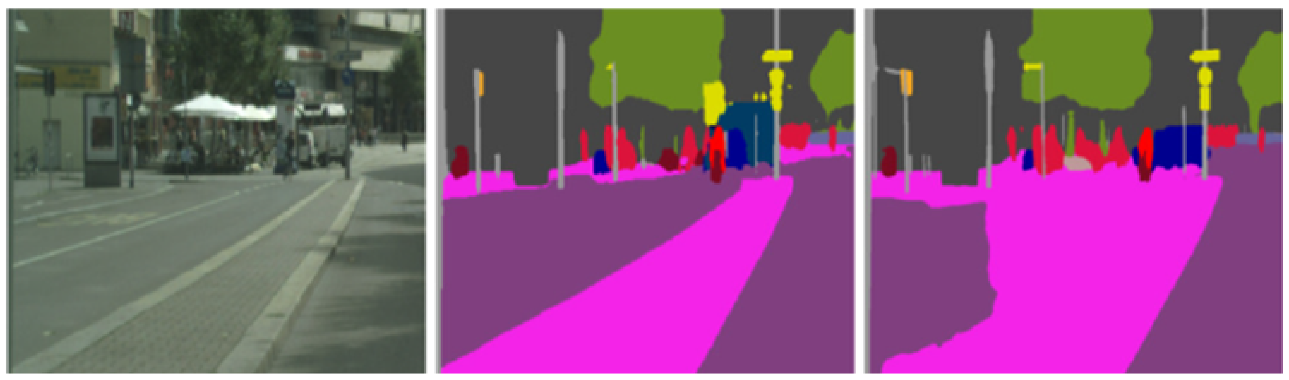
When applying semantic segmentation networks to real-world applications for safety issues, it is a problem that there are no clear criteria to judge failure cases. In other words, allowing the system to detect failures is important for self-driving [25,26,27] in autonomous driving systems. For example, predicted semantic segmentation map from neural network, Figure 1 (right), displays the misrecognition of the sidewalk as a lane. If such misconception occurs in the network of actual autonomous driving vehicles, it can function as a fatal flaw which leads to serious accidents (e.g., fatality or car accident). Therefore, the function of notifying them and handing over authority to drivers is essential when the driving system has delivered the wrong results to drivers. To prevent such accidents, we propose a neural network method by predicting the mean intersection of union (mIoU), which is a widely used evaluation metric in the semantic segmentation task, indicating how accurately each pixel of the image is classified.
1.2. Background Theory
Before describing our proposed failure detection and mIoU prediction framework, this section briefly reviews the fundamental theories related to the proposed method. We first briefly examine the theory of deep learning and then explain the neural network architecture that exhibits good image classification performance. Then, we review the semantic segmentation network and failure detection network used in this paper.
1.2.1. Deep Neural Network
Deep neural network (DNN) is an artificial neural network consisting of several hidden layers between the input and output layers which models complex nonlinear relationships. Additional layers help convergence of the features by gradually assembling lower layers.
Previous DNNs [28] have usually been designed as front-feed neural networks, but recent studies have successfully applied deep learning structures for various applications with standard error backpropagation algorithms [29,30]. Moreover, weights can be updated using the stochastic gradient descent via the equation below:
where indicates learning rate and C denotes the cost function. The selection of the cost function depends on the learning objectives and data.
1.2.2. Convolutional Neural Network
While conventional machine learning methods extract hand-crated feature, CNN needs minimal preprocessing. CNN consists of one or several convolutional layers with additional weights and pooling layers. These structures allow the CNN to make full use of the input data from a two-dimensional structure and train by using standard backpropagation. CNN is used as a general structure in various imaging and signal processing techniques and multiple benchmark results for standard image data. This section details the structure and role of CNN.
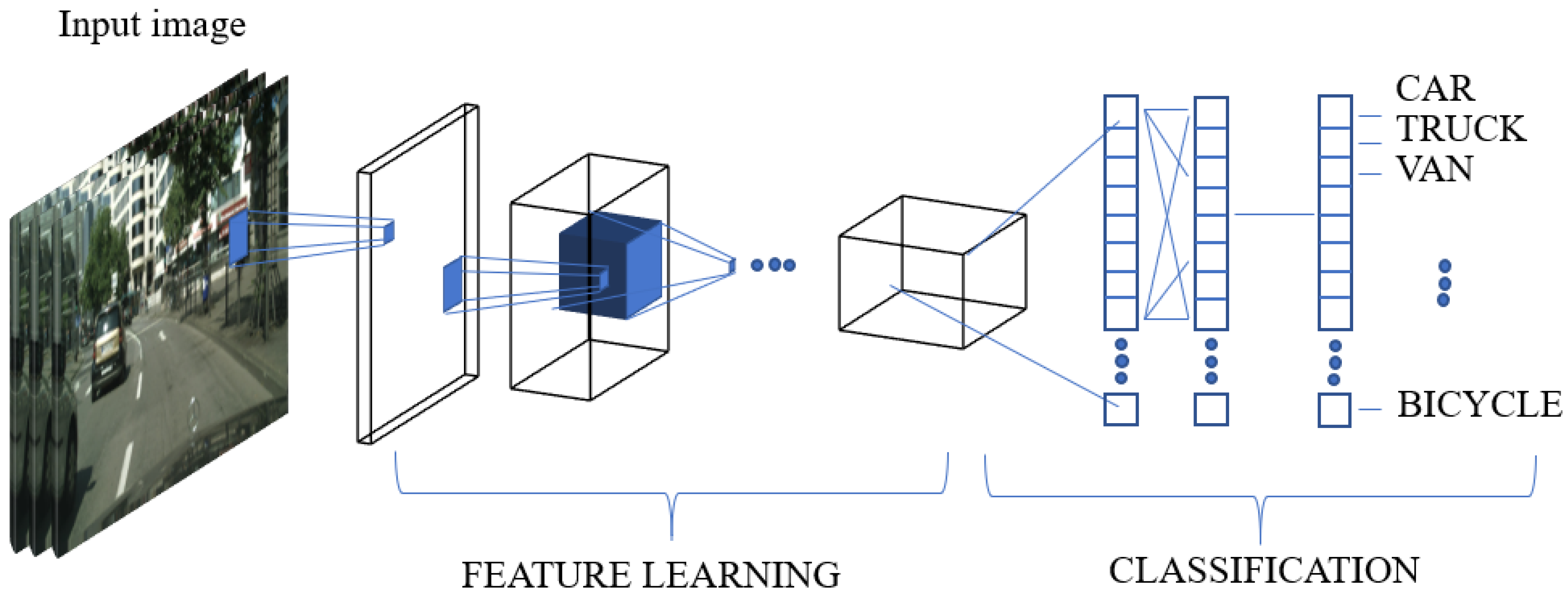
Convolutional layers are the vanilla blocks of the CNN. As shown in Figure 2, the network is divided into feature extracting part and classifying part. Feature extraction area comprises several convolutional and pooling layers. The convolutional layer is an essential element that applies a filter to the input data and reflects the activation function with an optional pooling layer. After the convolutional layers extract features, the fully connected layer (FCL) classifies the image using the extracted features. A flattening layer is placed between the part that extracts the image features and the one that classifies the image.
1.3. Research Objective and Contribution
This paper aims to predict mIoU of an image using semantic segmentation maps and design a network to determine whether it belongs to a failure case. In this study, we propose a two-stage network algorithm which evaluates the score to detect the failure case for the image input. First, the encoder network Efficient Spatial Pyramid of Dilated Convolutions for Semantic Segmentation (ESPNet) [31] extracts features for the image and semantic segmentation map. Second, failure cases of the segmentation network are detected by FCL for mIoU prediction of images through the proposed methods. As a result, the proposed method can be used as a basis for a fully autonomous driving system to allow self-diagnosis. Our main contributions can be summarized as follows:
- We secure safety by proposing a failure detection network for image segmentation.
- Our model simultaneously performs mIoU prediction and failure detection for a single image.
- We propose a modified loss function to solve the data imbalance problem of the generated ground-truth (GT) mIoU.
- The proposed model exhibits good performance not only on the Cityscapes dataset but also on the Hyundai Motor Group (HMG) dataset.
The remainder of the paper is organized as follows. Section 2 describes the complete process of our mIoUNet method and analyzes the structure of the model. Section 3 presents the experimental results using various network structures and the various input channels. The challenge dataset verifies the robustness of the network using the surround-view monitoring (SVM) camera road image provided by HMG. Finally, the paper ends with the conclusion in Section 4.
2. Proposed Failure Detection Network
In this section, we propose a network called mIoUNet that predicts the mIoU for images and detect failure. The learning pipeline of the proposed algorithm is as follows. First, we fully explain the how the training data are generated. Secondly, we show the optimized network structure that suits our purpose. Then, the details of CNN and FCL are introduced including the activation function and loss function. Finally, modified the loss function is introduced for failure detection task.
2.1. Data Generation
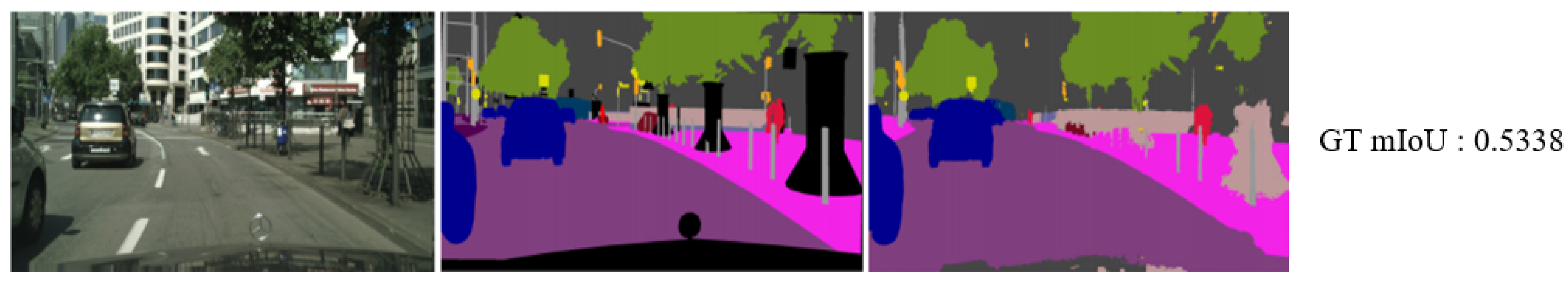
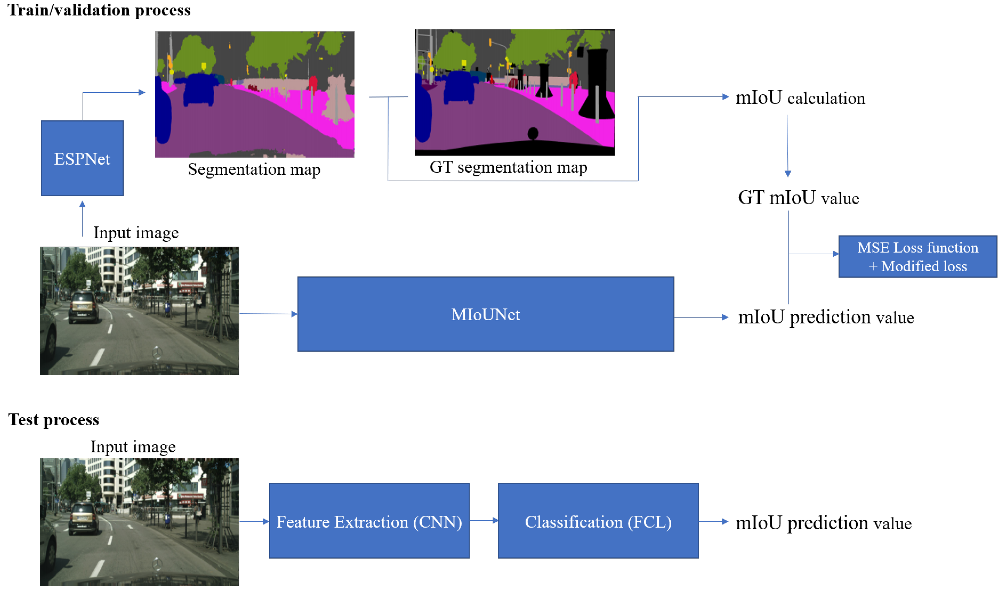
We define the terms used in this paper as follows. The GT segmentation map is ground truth of a semantic segmentation example. The GT mIoU is calculated by comparing the GT segmentation map with predicted segmentation map from the segmentation network. An example can be seen in Figure 3. The right side of the figure shows a segmentation map image which was generated using the ESPNet in Figure 3 (left), while the middle figure shows the GT segmentation map. After extracting segmentation maps, GT mIoU values are calculated in the form of a scalar value.
2.2. Selection of the Convolutional Neural Network Structure
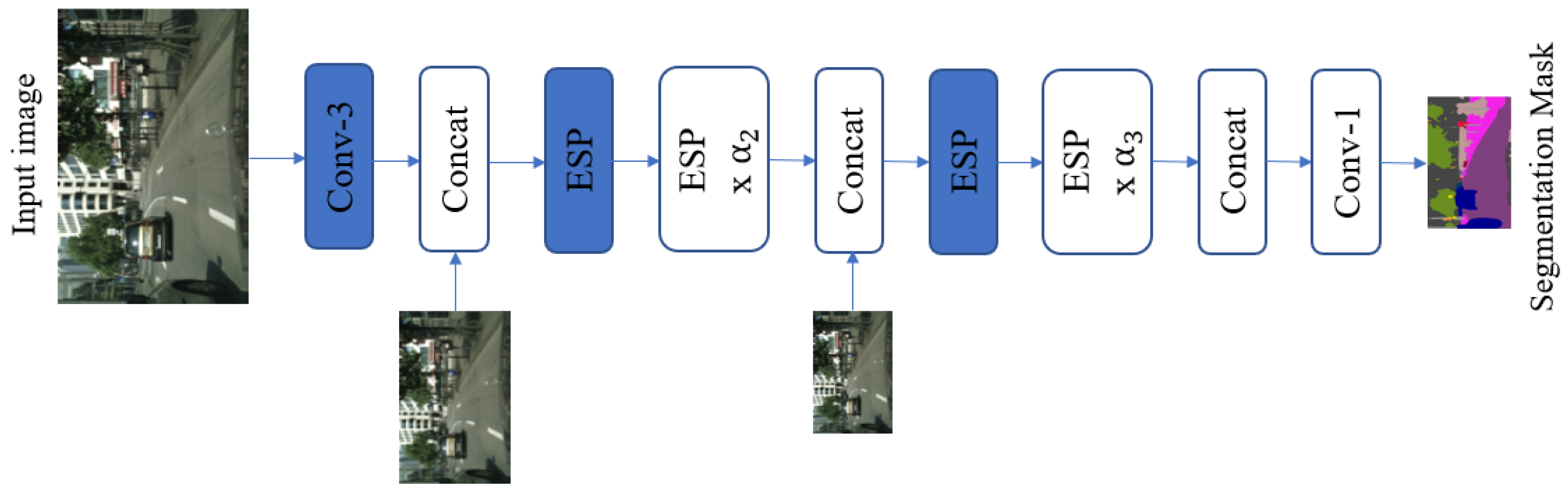
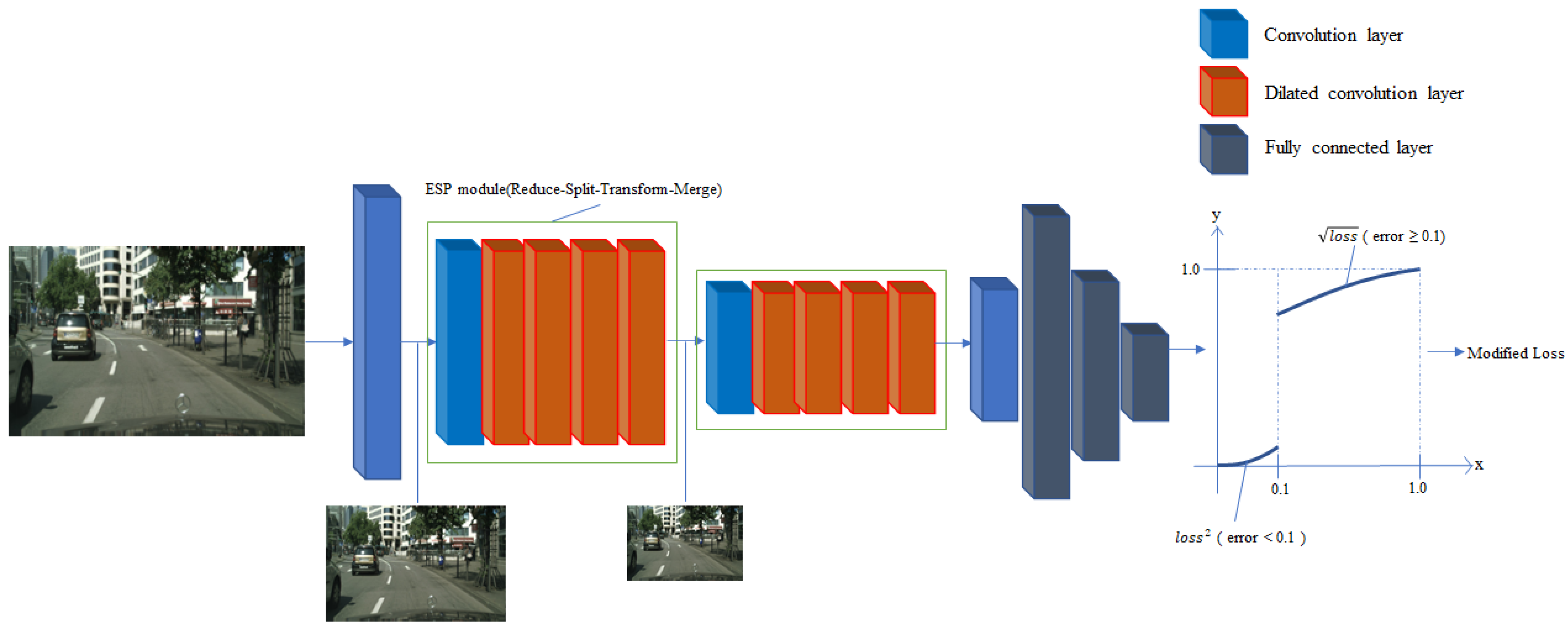
Our mIoUNet structure consists of a front part composed of the CNN, which performs feature extraction, and a back part composed of FCL for failure detection. In this paper, we propose an end-to-end network with sigmoid function at the end. Our main segmentation network is ESPNet, which is a segmentation network of a reduction-split-transform-merge structure using convolutional factorization. Similarly, mIoUNet uses the encoder part of ESPNet to extract similar feature from same structure, as illustrated in Figure 4.
2.3. Selection of the Fully Connected Layer Structure
In image classification, the structure of FCL is selected by referring to the experimental results of the performance by changing number of layers and nodes [32]. To select the best structure of mIoUNet, experiments were conducted with various layers and nodes with the highest accuracy. Table 1 presents 10 different cases [32] of the FCL structures and their results. CNN-2 structure is used, which is most similar to ESPNet-C. More details are provided in Section 3.3.
2.4. Selection of the Activation Function
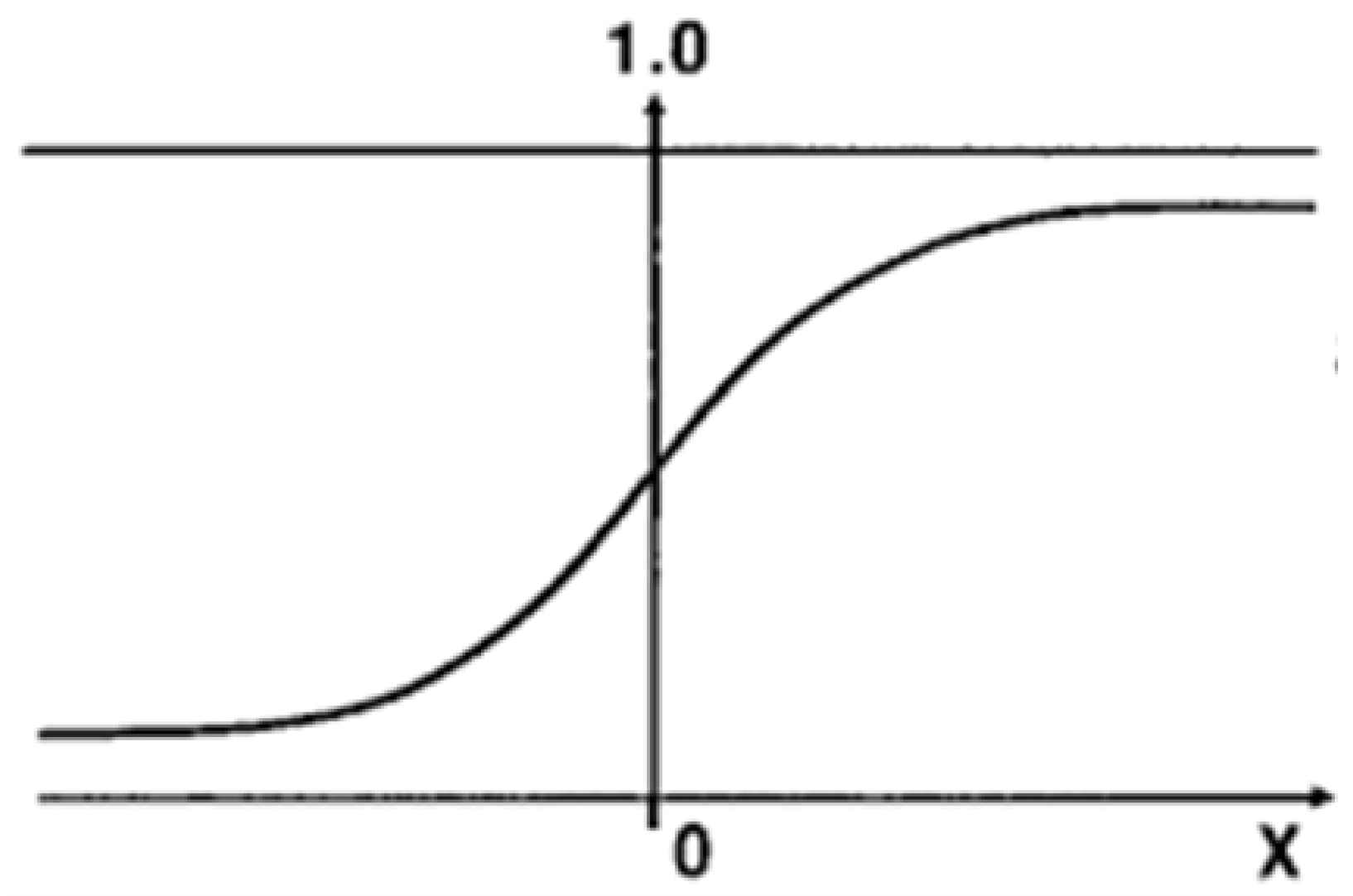
The Sigmoid function is used at the end of the FCL. As illustrated in Figure 5, the function has outputs value between 0 and 1; therefore, it is suitable for predicting mIoU values.
2.5. Selection of the Loss Function
The difference between the predicted mIoU and GT mIoU values obtained through the model is defined as the loss, and the network tries to learn to by minimizing the loss. Mean squared error (MSE) is selected to calculate the loss value between scalar values.
where denotes the predicted mIoU value and indicates the GT mIoU value.
2.6. Modified Loss Function
In the initial version, mIoUNet was trained with MSE as a loss function, but prediction for the testing set converged near 0.5. In other words, mIoUNet did not detect out of range mIoU values. As a result of analyzing the data to determine the cause, imbalance distribution of GT mIoU was composed, as depicted in Table 2.
As shown in Table 2, the GT mIoU value of the test set distributed between 0.4 and 0.6 was 394, 78.8% of the total data. Such cross imbalance on data made the model overfit the prediction for mIoU values between 0.4 and 0.6. The MSE learning problem is that the data are concentrated around 0.5; the tendency is to follow the average simply to minimize the MSE loss value. Therefore, the loss value was modified as follows for learning.
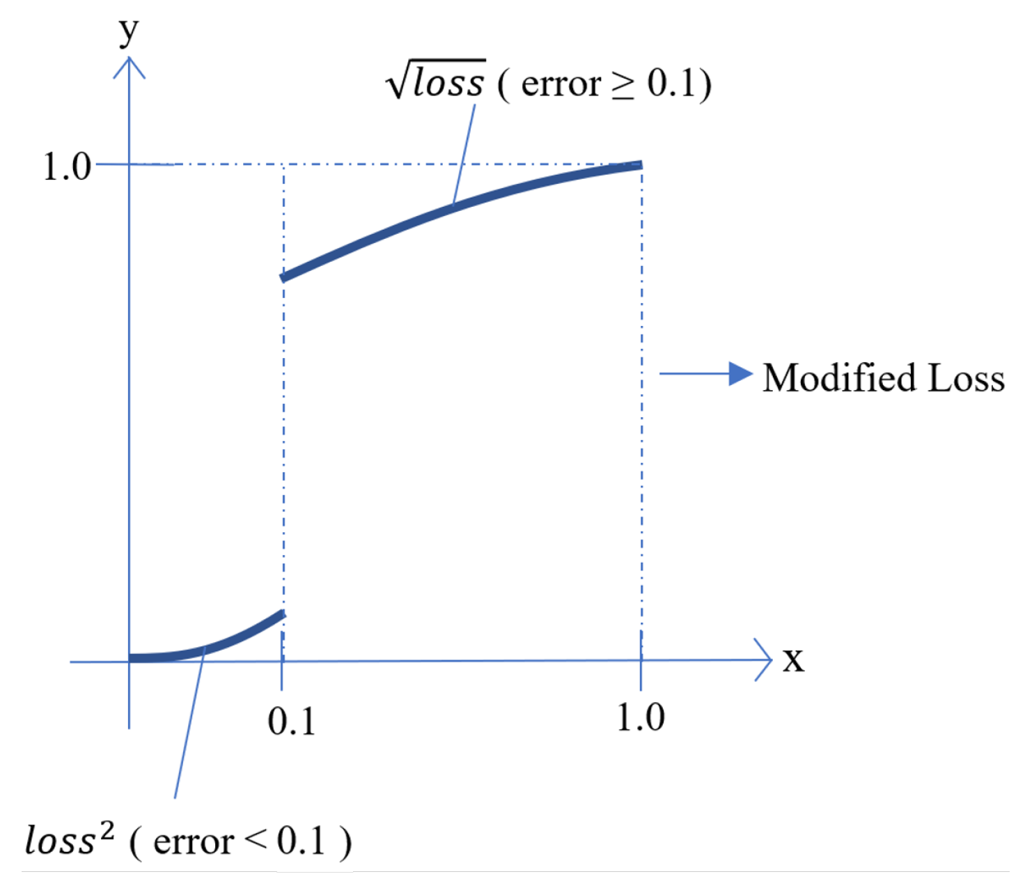
The new modified loss corrects the overfitting problem by minimizing the effect on outliers for robustness in normal networks. When the difference between the actual and scalar value is less than 0.1, the transformed loss value is squared by the initial loss value, and, when it is greater than 0.1, the original loss value is square-rooted. As shown in Figure 6, in the case of a loss calculated less than the value of 0.1 as the error margin, a smaller loss value is used. In the opposite case, a larger loss value is used to allow the optimizer to backward error:
2.7. Final Network Structure
Our proposed model structure is shown in Figure 7 and Figure 8. Figure 7 depicts the training, validation, and test process of the pipelines. Figure 8 presents the overall architecture of proposed model. Network details such as layer structure are described in Table 3.
In the case of semantic segmentation, the intersection of union (IoU) value becomes the denominator of the number of pixels corresponding to any class and the number of pixels accurately predicted for that class. The average value is called mIoU. In this paper, we compute the mIoU between the GT segmentation map and the segmentation map obtained via ESPNet to obtain the GT mIoU value.
3. Experimental Results
We conducted extensive experiments to demonstrate the performance of our proposed network. For performance evaluation, the prediction accuracy of the mIoU value of the image in the testing set was calculated, and the accuracy of the failure detection was calculated through the predicted mIoU value. The mean absolute error (MAE) was used as the evaluation metric to calculate the error because, when calculating positive and negative numbers, the meaning may be canceled out.
The MAE is calculated as follows:
where denotes the predicted mIoU value and indicates the GT mIoU value.
The mIoU prediction accuracy is calculated as follows:
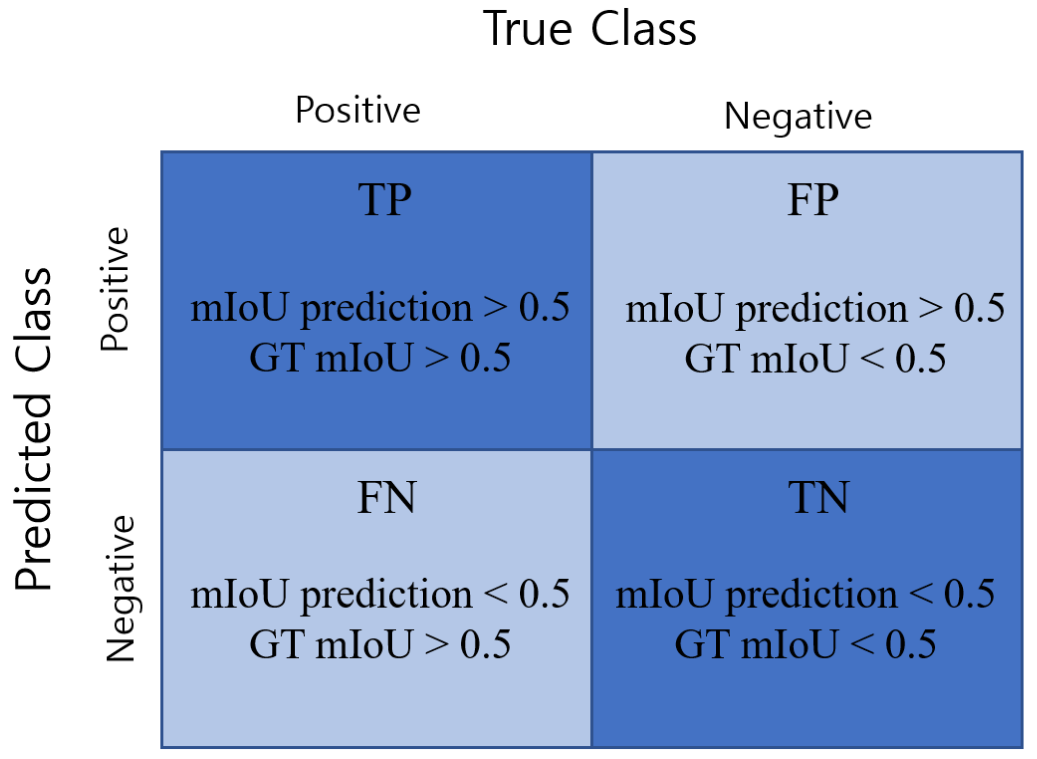
Failure detection accuracy is calculated as follows. The precision, recall, and F1-score values are considered simultaneously to determine whether the detection result is reasonable. The method of calculating the performance indicators can be easily understood in Figure 9.
The results of the experiment are classified into each situation according to the following criteria: True positive (TP) and true negative (TN) are the cases when the performance of ESPNet is well predicted by mIoUNet. In more detail, TP is defined when the mIoU prediction value and the GT mIoU value are greater than a threshold value of 0.5 where TN is smaller than 0.5. In both cases, the mIoUNet successfully detects not only the failure case but also success case for ESPNet. On the other hand, false positive (FP) and false negative (FN) are when mIoUNet fails to predict the failure or success case of ESPNet. FP is defined as the mIoU prediction value is larger than 0.5, but the GT mIoU prediction value is less than 0.5. On the contrary, FN is defined as the mIoU prediction value is smaller than 0.5, but the GT mIoU prediction value is greater than 0.5. In both cases, we define that the mIoUNet fails to detect properly the failure cases and success cases.
The evaluation metrics for failure case detection are calculated as follows:
3.1. Experimental Setup
In this subsection, we analyze our experimental results to evaluate the performance of the proposed algorithm on Cityscapes and Hyundai Motor Group (HMG) dataset. After each convolutional layer in the CNN, a batch normalization [33] and a rectified linear unit [5] layer are applied. Adam optimizer method [34] is used for training with batch size of 12 for 30 epochs. The size of the network input was set to . Initial learning rate starts from 0.0001 and halving every 10 epochs. Dropout [35] is applied at a ratio of 0.5. All experiments were conducted on an NVIDIA Tesla V 100 implemented with PyTorch library.
3.2. Datasets
Two datasets were used in the experiment. The first is the Cityscapes dataset, a widely used segmentation dataset, which includes 2975 images for the training/validation set and the testing set contains 500 images. The second, vertical image, dataset for the road area was obtained by attaching an SVM camera to an actual vehicle from HMG. It consists of 863 images in the training/validation set and 216 in the testing set. To check the network robustness, we applied our method to rain/haze images and real-world road images, which are treated as different domains.
3.3. Experimental Results
3.3.1. Quantitative Results
Various FCL structures were applied to predict mIoU values and used in our task. According to the various FCL structures, the evaluation indicators are as follows: selecting the most efficient model, mIoU prediction accuracy, number of parameters, and run time.
Similar to the image classification in [32], as the number of nodes in the FCL increases, the mIoU prediction accuracy becomes higher. However, real-time detection must be guaranteed. Therefore, 256-20-1, a structure with high accuracy that does not require a run time of 1 s, was selected. The evaluation indices obtained using the selected network structure are shown in Table 4. The mIoU prediction accuracy was calculated using (5) and (6).
Experiments were conducted in two directions using the selected network structure:
- Additional information: Additional information is learned by increasing the number of channels to improve prediction performance. We experimented with the cases of RGB, RGB hue, and RGB segmentation (RGBSeg) to observe the difference when learning additional information.
- Real-time application: The image size was reduced and trained to secure real-time performance.
In adding one more channel with additional information, the accuracy improved when adding a hue channel corresponding to the color and adding a segmentation map. The increase in run time due to the increased network parameters as the channel was added was insignificant. We decided to use an input image with four RGB channels and a segmentation map for the best results (Table 5).
After fixing the input image with RGBSeg with four channels, the input size was adjusted to reduce the network parameters. The experiments were conducted by reducing the existing 1024 × 512 input image to two times and four times. As the computation amount was reduced, the run time was similarly reduced with a real-time application, but the accuracy also decreased (Table 6).
As expected, when the image size was the largest, the accuracy was highest, and, when the image size was halved, the accuracy decreased by about 1.2%. The detection results of the limit situations according to each input size of the image are listed in Table 7.
The accuracy of failure detection significantly decreased as the input size decreases. However, as presented in Table 7, the precision, recall, and F1-score values were calculated to determine why the mIoU prediction accuracy was higher than 512 × 256. As a result of checking the value, the image size was reduced so much that the network could learn much less, and training was performed to reduce the loss function. Therefore, all testing set images were recognized as failures due to overfitting on most GT mIOU values. In addition, when comparing the results for images of size 1024 × 512 and 512 × 256, the accuracy difference is almost 15%. Although the run time differed by about 2.7 times, the detection accuracy was significantly lower; therefore, it was not efficient to reduce the input size of the image to provide real-time characteristics.
The accuracy of MSE loss function and the accuracy of modified loss function differ as follows (Table 8). As a result of comparison, the loss function that fits well with the characteristics of unbalanced data was used to confirm 4.6% accuracy improvement for failure detection and 2.3% for mIoU prediction. The mIoU prediction accuracy is obtained using (5) and (6). Failure detection accuracy was calculated using (7).
3.3.2. Qualitative Results
This section shows examples of mispredicted Cityscapes dataset images among the results classified by the mIoUNet. The qualitative test results show the input image, GT segmentation map, and segmentation map for the testing set at the same time, as well as the GT mIoU, mIoU prediction, mIoU error value and failure detection result of the image.
False-Negative Image
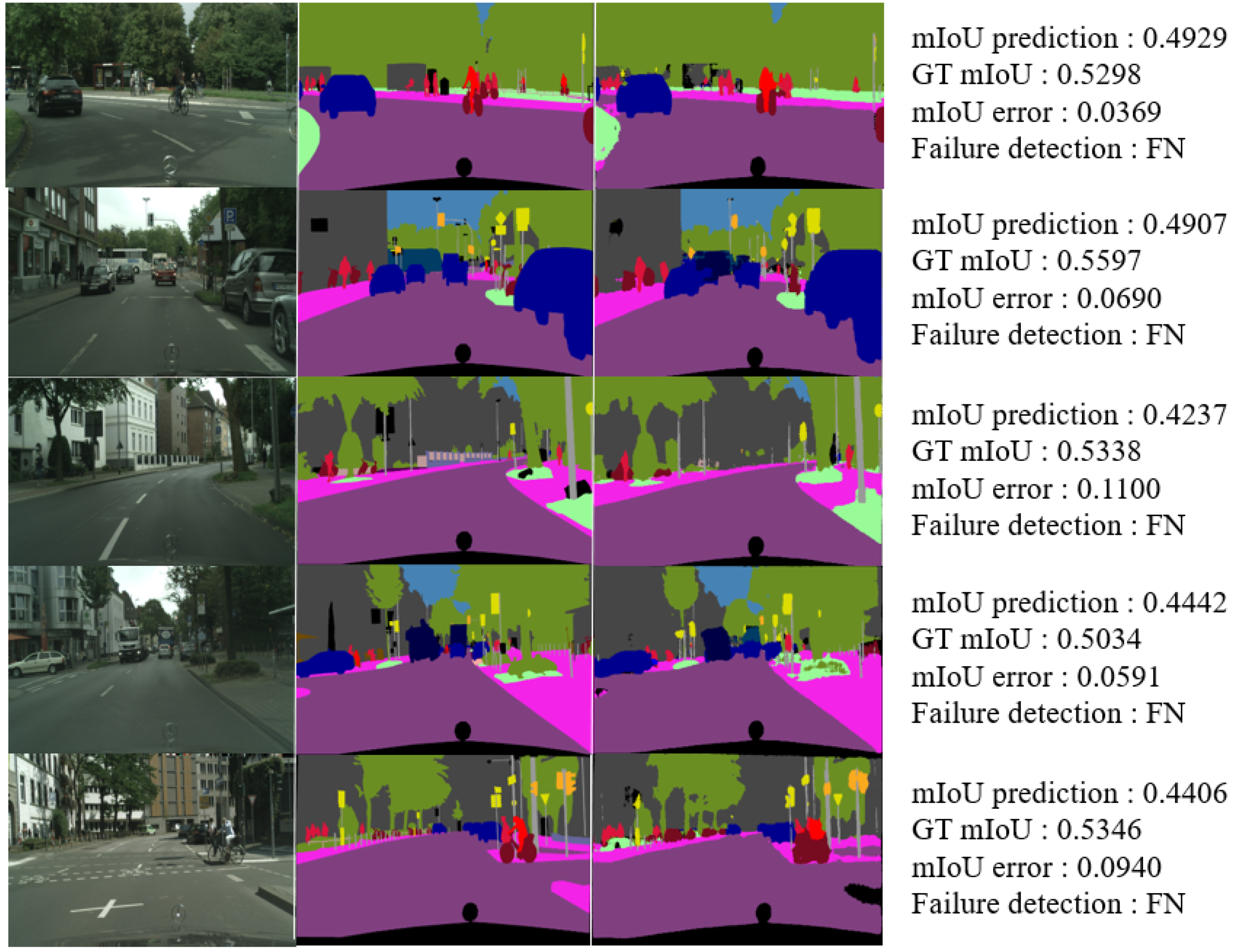
Figure 10 presents examples of results classified as false-negative images. Figure 10 (left) displays input images, and Figure 10 (middle) displays segmentation maps. Out of the 500 images, 27 images were detected. The false negative refers to when the GT mIoU is greater than 0.5 and the mIoU prediction is less than 0.5. The MAE values for mIoU of these images are as follows.
If the network is used for the actual autonomous driving function, convenience can be increased by allowing the MAE value that defines the limit situation to be set according to users’ convenience.
Table 9 demonstrates that false-negative images have a small error. In particular, the average error was 0.075, which is smaller than the error value of 0.1, which is defined as the failure cases.
False-Positive Image
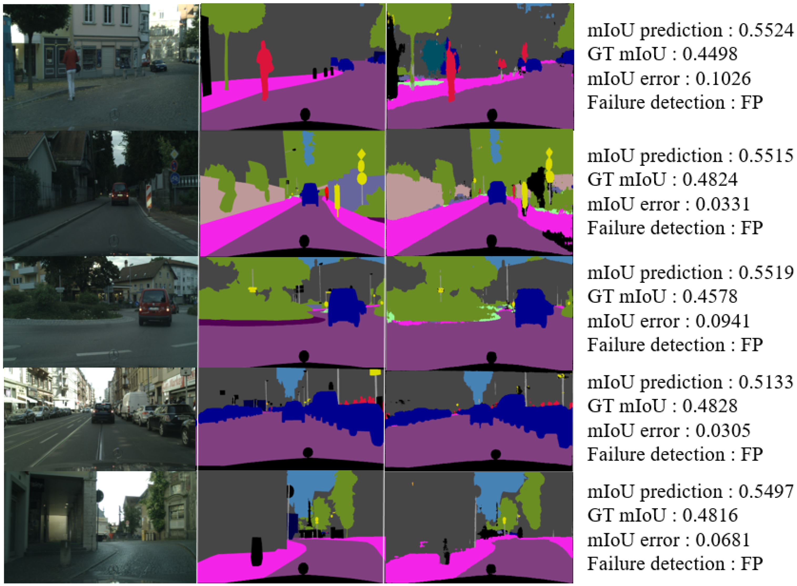
Figure 11 is an example of a result identified as a false-positive image. The first column of Figure 11 depicts the input images, and the second column of Figure 11 depicts the segmentation maps. Total 42 from 500 samples. The false-positive case is when the GT mIoU is less than 0.5, and the mIoU prediction is greater than 0.5. The MAE values for the mIoU of these images are as follows.
Table 10 demonstrates that false-positive images have larger error values than false-negative images. The average error of the images was calculated as 0.045, and the max error was 0.5. To determine the cause, the images that make the average error higher are classified separately.
Failure Cases
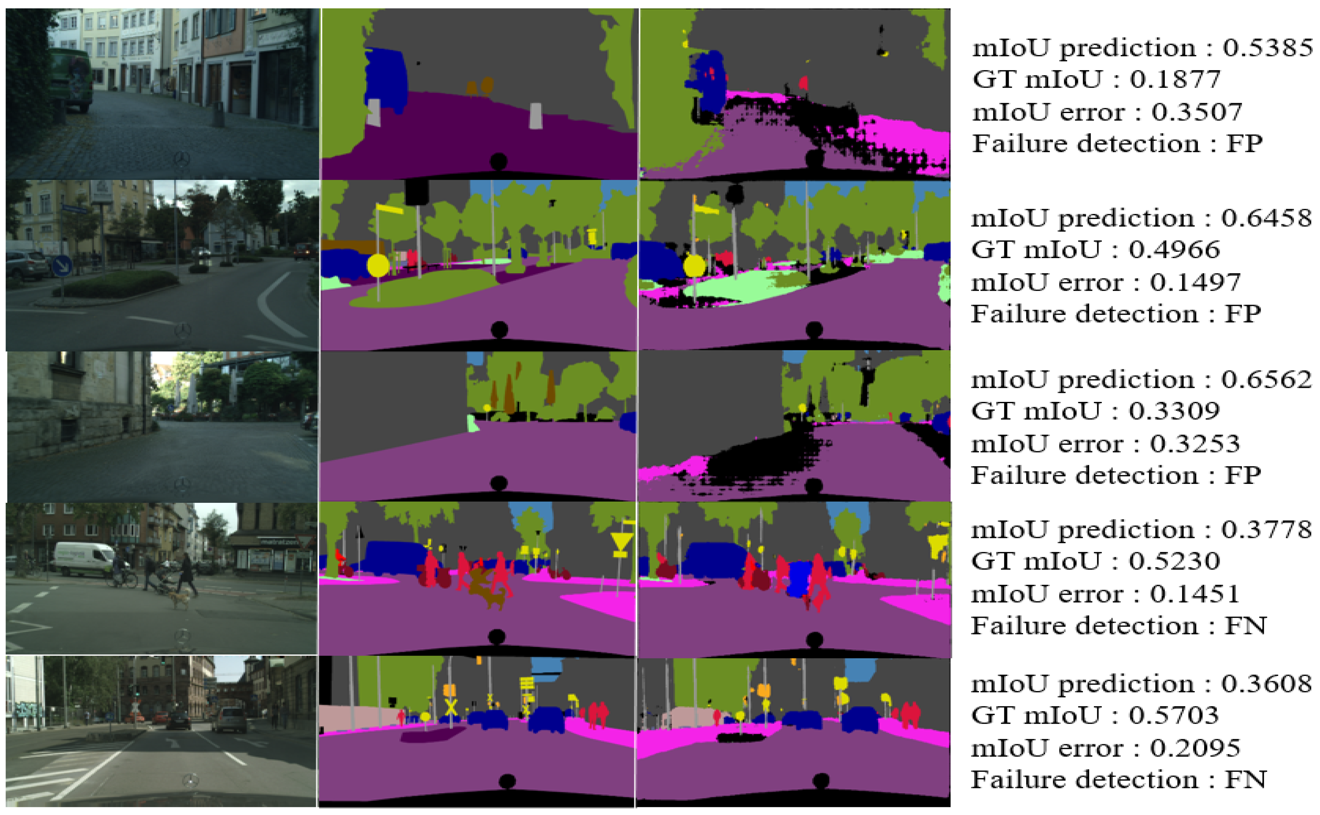
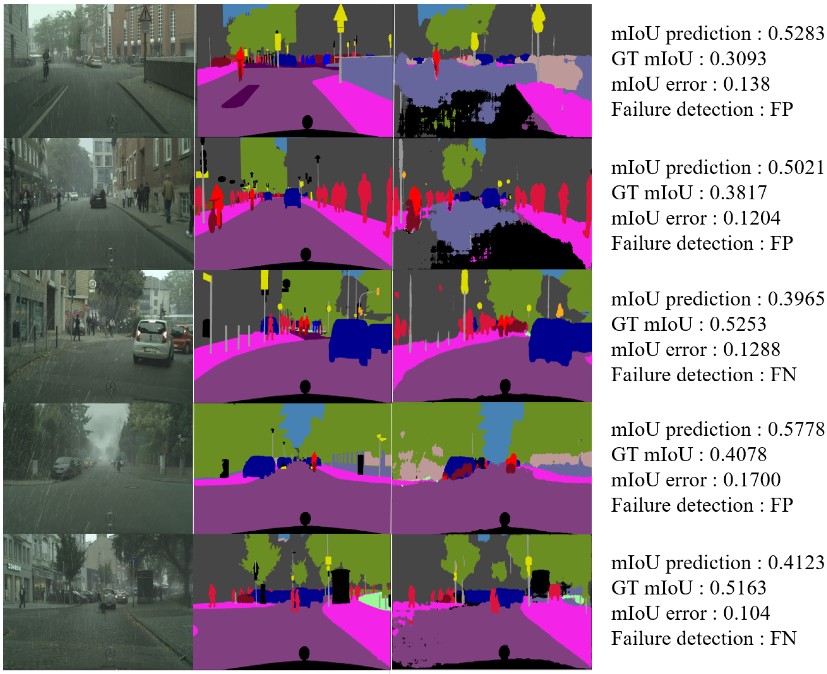
Figure 12 presents six images with large error values. The first column of Figure 12 displays the input images and the second column of Figure 12 displays the segmentation maps. First, some cases had many pixels in the image that were not considered a class in the segmentation map. In the semantic segmentation process on the right side of each picture, the area shown as black is the area deduced as pixels with no class. This dramatically decreases the GT mIoU value when calculating the mIoU value. This phenomenon is solved by randomly assigning classes by handling exceptions during the semantic segmentation inference or by inference using a better semantic segmentation network. Second, there are few pixels in the general roadway area in the image. For example, one can see narrow roads, roads with severe curvature and alleyways with many other buildings and structures. This problem can be solved by assigning more weight to pixels corresponding to classes, such as roads, people, and obstacles, which are essential in safe driving when the network is learning.
3.4. Experimental Results on the Rain/Haze Dataset
Experiments were conducted with images from the rain/haze composite version of the Cityscapes dataset (Figure 13). This can be viewed in the same domain but in a different environment. The quantitative test result is the average of all the result values for the testing set. The qualitative test results show the input image, GT segmentation map, and segmentation map for the testing set at the same time, as well as the GT mIoU, mIoU prediction, mIoU error value, and failure detection result of the image.
3.4.1. Quantitative Results
The official RainCityscapes dataset [36] is composed of 66 images with different rain and haze versions. The experiments confirm that no significant difference exists based on RainCityscapes. We randomly used images corresponding to the various hyperparameters of the dataset in the experiments. mIoUNet detected 14 of 66 images as limit situations. Although a slight performance decline occurred due to the effects of rain and haze, the model is generally robust to other environments. mIoU prediction accuracy and the Failure detection accuracy for rain/haze dataset are shown in Table 11.
3.4.2. Qualitative Results
Examples of images detected as failure cases are presented in Figure 13. These images are also detected as failure cases when there are few road areas or many obstacles and buildings.
3.5. Experimental Results on the DeepLabV3+ Model
We experimented with DeepLabV3+ [20] to ensure that the proposed method is also applicable to other semantic segmentation models. We conducted an experiment to ensure that performance is maintained even when using GT mIoU values generated by other segmentation models after fixing the structure of the network, which is the second step of our network structure. Table 12 represents the distribution of GT mIoU values generated using DeepLabV3+ models.
The results of the learning using MSE and the modified loss function are shown in Table 13. As the shown in the table, the proposed loss function shows improved performance, but not as much as using ESPNet in Table 8. This is likely because the distribution of GT mIoU using DeepLabV3+ models has lower variance than that of ESPNet. However, a slight performance improvement was shown in the accuracy of failure detection and mIoU predication. We confirm that the proposed loss function not only results in significant performance improvements in unbalanced data, but also performs well in data from other distributions.
3.6. Experimental Results on the Challenging Dataset
We experimented with HMG dataset, which has a different viewpoint from Cityscapes. This dataset used a SVM camera road image dataset. It consists of 1079 road images acquired by an SVM camera attached to a vehicle, provided by Hyundai Motor Group. The experimental environment is the same as previously described. However, the last of the FCL is set to 12 because the number of segmentation classes is 12. Training set and validation set comprised 80% (863 images), and the remaining 20% (216) of the images were used as the testing set. Considering that the total number of images is 1079, which is less than that of the Cityscapes dataset, the learning rate was reduced by half every 50 epochs with 150 total epochs of training. The GT mIoU value distribution of HMG dataset was composed as depicted in Table 14.
3.6.1. Quantitative Results
In the case of HMG dataset, we experimented with the use of loss function as MSE and the application of modified loss function (Table 15). The table shows that using the modified loss function gives better performance on both Cityscapes and HMG dataset.
The results of different experiments on the number of input channels are shown in Table 16.
Due to the dataset characteristics, it is necessary to change mIoU value to set it as the failure case. In addition, 0.6 was set as the threshold value of the mIoU corresponding to the failure case, where all performance indicators are generally good as following Table 17.
3.6.2. Qualitative Results
This section presents examples of mispredicted HMG dataset images among the results classified by mIoUNet.
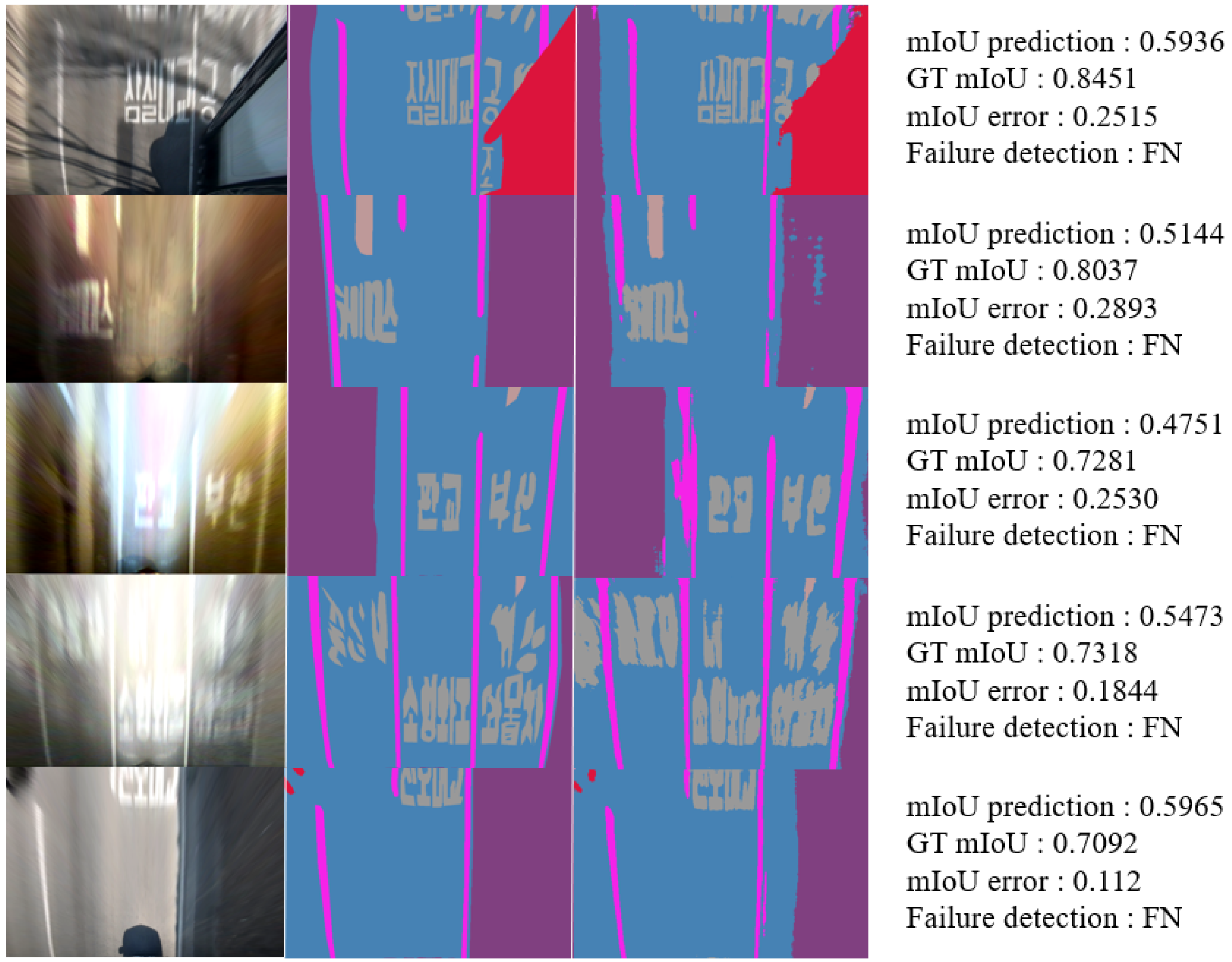
False-Negative Image in the HMG Dataset
The first column of Figure 14 depicts the input images, and the second column of Figure 14 depicts the segmentation maps. In the case of false-negative images (Figure 14), many images were taken during the day, and the degree of light dispersion was large within one image. For example, images with shadows and images with lights shining on a tunnel were classified.
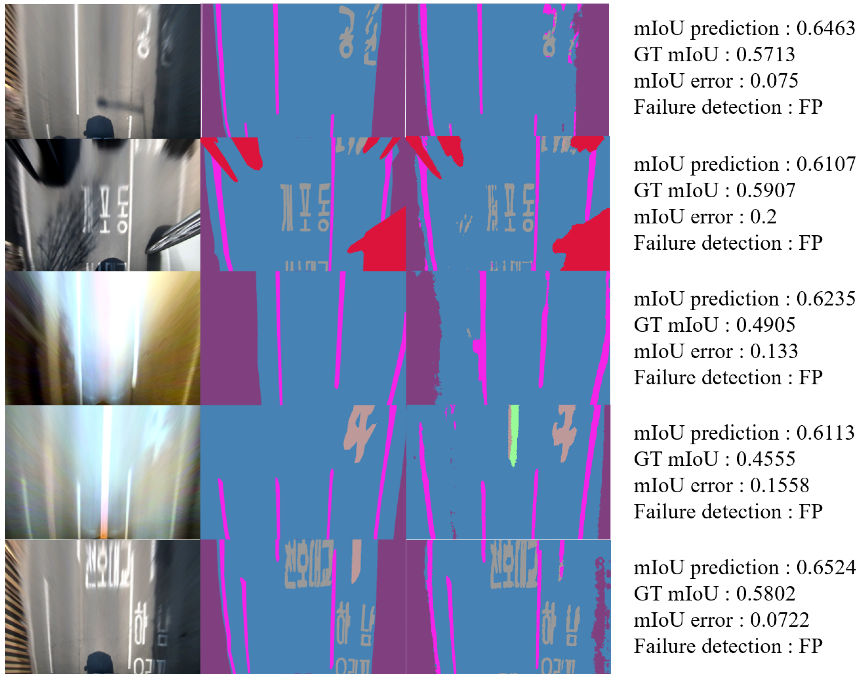
False-Positive Image in the HMG Dataset
The first column of Figure 15 presents the input images, and the second column of Figure 15 presents the segmentation maps. In the case of false-positive images, many images were taken at night, and the images with high light dispersion were detected. The difference from the false-negative image is that many images were detected when the edge information, such as road markers or lanes, was not adequately visible or was in the road area. To summarize the results, the proposed model has a problem in that the mIoU cannot be accurately predicted when the light change is considerable in the vertical image of the road. However, the qualitative evaluation results reveal that using additional information, such as edges, can increase prediction accuracy.
4. Conclusions
In the image recognition system of an autonomous vehicle, for safety, it is crucial for the system to judge the failure cases autonomously, which is a standard for Level 3 autonomous driving. This paper proposes failure detection network for road images segmentation using mIoU. Our mIoUNet uses CNN and FCL, which are commonly used in the existing classification network structure.
The results on the Cityscapes dataset reveal 93.21% mIoU prediction accuracy and 84.8% failure detection accuracy. As a challenging task, HMG’s SVM camera acquisition dataset, which is taken from different viewpoints, demonstrated 90.51% mIoU prediction accuracy and 83.33% failure detection accuracy.
As a result of experimenting with many different FCL structure versions, an efficient 256 × 12 × 1 FCL structure with high accuracy and fast inference speed is implemented and assessed with a model trained using a modified loss function. Performance of the network improved due to an increase in the number of input channels. This phenomenon means additional information is provided and detecting failure situations can be improved.
Finally, as a result of analyzing pictures with terrible error values, we observed that the proposed model successfully detects failure cases. We note the possibility that the performance of the proposed network can be improved according to the performance of semantic segmentation that creates the GT mIoU. This result suggests that a more accurate and robust semantic segmentation model results in better performance of the proposed model.
Although it is meant to detect failure cases in road images in autonomous driving, the proposed method only evaluated the reliability of single images. We aim to study a failure detection network that can predict the reliability of each pixel in an image as future work. Lightening the network structure to ensure real-time performance can also be considered as a future work.
Author Contributions
Conceptualization, J.S. and W.A.; methodology, S.P. and M.L.; software, J.S. and W.A.; validation, J.S. and W.A.; formal analysis, J.S.; investigation, J.S. and W.A.; resources, J.S.; data curation, J.S.; writing—original draft preparation, J.S.; writing—review and editing, J.S. and W.A.; visualization, J.S.; supervision, M.L.; project administration, M.L.; and funding acquisition, J.S. and M.L. All authors have read and agreed to the published version of the manuscript.
Funding
This research was supported by the Hyundai Motor Group (HMG) funded by the Hyundai NGV and in part by the Basic Science Research Program through the National Research Foundation of Korea (NRF) (Grants No. NRF-2016R1D1A1B01016071).
Data Availability Statement
The Cityscapes data presented in this study are openly available in Cityscapes paper [37]. Hyundai Motor Groups data sharing is not applicable to this article.
Conflicts of Interest
The authors declare no conflict of interest.
References
- He, K.; Zhang, X.; Ren, S.; Sun, J. Identity mappings in deep residual networks. arXiv 2016, arXiv:1603.05027. [Google Scholar]
- He, K.; Gkioxari, G.; Dollár, P.; Girshick, R. Mask r-cnn. arXiv 2017, arXiv:1703.06870. [Google Scholar]
- Dai, J.; Qi, H.; Xiong, Y.; Li, Y.; Zhang, G.; Hu, H.; Wei, Y. Deformable convolutional networks. arXiv 2017, arXiv:1703.06211. [Google Scholar]
- Luan, F.; Paris, S.; Shechtman, E.; Bala, K. Deep photo style transfer. arXiv 2017, arXiv:1703.07511. [Google Scholar]
- Krizhevsky, A.; Sutskever, I.; Hinton, G.E. Imagenet classification with deep convolutional neural networks. Adv. Neural Inf. Process. Syst. 2012, 25, 1097–1105. [Google Scholar] [CrossRef]
- Srivastava, R.K.; Greff, K.; Schmidhuber, J. Training very deep networks. arXiv 2015, arXiv:1507.06228. [Google Scholar]
- He, K.; Zhang, X.; Ren, S.; Sun, J. Delving deep into rectifiers: Surpassing human-level performance on imagenet classification. arXiv 2015, arXiv:1502.01852. [Google Scholar]
- Hinton, G.E.; Srivastava, N.; Krizhevsky, A.; Sutskever, I.; Salakhutdinov, R.R. Improving neural networks by preventing co-adaptation of feature detectors. arXiv 2012, arXiv:1207.0580. [Google Scholar]
- Bergstra, J.; Bengio, Y. Random search for hyper-parameter optimization. J. Mach. Learn. Res. 2012, 13, 281–305. [Google Scholar]
- Szegedy, C.; Vanhoucke, V.; Ioffe, S.; Shlens, J.; Wojna, Z. Rethinking the inception architecture for computer vision. arXiv 2016, arXiv:1512.00567. [Google Scholar]
- Szegedy, C.; Ioffe, S.; Vanhoucke, V.; Alemi, A. Inception-v4, inception-resnet and the impact of residual connections on learning. arXiv 2016, arXiv:1602.07261. [Google Scholar]
- Zhang, W.; Ma, K.; Yan, J.; Deng, D.; Wang, Z. Blind image quality assessment using a deep bilinear convolutional neural network. IEEE Trans. Circuits Syst. Video Technol. 2018, 30, 36–47. [Google Scholar] [CrossRef] [Green Version]
- Lin, M.; Chen, Q.; Yan, S. Network in network. arXiv 2013, arXiv:1312.4400. [Google Scholar]
- Goodfellow, I.; Warde-Farley, D.; Mirza, M.; Courville, A.; Bengio, Y. Maxout networks. arXiv 2013, arXiv:1302.4389. [Google Scholar]
- Howard, A.G.; Zhu, M.; Chen, B.; Kalenichenko, D.; Wang, W.; Weyand, T.; Andreetto, M.; Adam, H. Mobilenets: Efficient convolutional neural networks for mobile vision applications. arXiv 2017, arXiv:1704.04861. [Google Scholar]
- Sermanet, P.; Eigen, D.; Zhang, X.; Mathieu, M.; Fergus, R.; LeCun, Y. Overfeat: Integrated recognition, localization and detection using convolutional networks. arXiv 2013, arXiv:1312.6229. [Google Scholar]
- Girshick, R.; Donahue, J.; Darrell, T.; Malik, J. Rich feature hierarchies for accurate object detection and semantic segmentation. arXiv 2014, arXiv:1311.2524. [Google Scholar]
- Redmon, J.; Divvala, S.; Girshick, R.; Farhadi, A. You only look once: Unified, real-time object detection. arXiv 2016, arXiv:1506.02640. [Google Scholar]
- Ren, S.; He, K.; Girshick, R.; Sun, J. Faster r-cnn: Towards real-time object detection with region proposal networks. arXiv 2015, arXiv:1506.01497. [Google Scholar] [CrossRef] [Green Version]
- Chen, L.C.; Zhu, Y.; Papandreou, G.; Schroff, F.; Adam, H. Encoder-decoder with atrous separable convolution for semantic image segmentation. arXiv 2018, arXiv:1802.02611. [Google Scholar]
- Wang, P.; Chen, P.; Yuan, Y.; Liu, D.; Huang, Z.; Hou, X.; Cottrell, G. Understanding convolution for semantic segmentation. arXiv 2018, arXiv:1702.08502. [Google Scholar]
- He, K.; Zhang, X.; Ren, S.; Sun, J. Spatial pyramid pooling in deep convolutional networks for visual recognition. IEEE Trans. Pattern Anal. Mach. Intell. 2015, 37, 1904–1916. [Google Scholar] [CrossRef] [Green Version]
- Chen, L.C.; Papandreou, G.; Kokkinos, I.; Murphy, K.; Yuille, A.L. Semantic image segmentation with deep convolutional nets and fully connected crfs. arXiv 2014, arXiv:1412.7062. [Google Scholar]
- National Highway Traffic Safety Administration. Automated Driving Systems 2.0: A Vision for Safety; US Department of Transportation, DOT HS: Washington, DC, USA, 2017; Volume 812, p. 442.
- Pires, I.M.; Garcia, N.M. Identification of Warning Situations in Road Using Cloud Computing Technologies and Sensors Available in Mobile Devices: A Systematic Review. Electronics 2020, 9, 416. [Google Scholar] [CrossRef] [Green Version]
- Sharma, D.; Pandit, D. Determining the level of service measures to evaluate service quality of fixed-route shared motorized para-transit services. Transp. Policy 2021, 100, 176–186. [Google Scholar] [CrossRef]
- Jang, J.A.; Kim, H.S.; Cho, H.B. Smart roadside system for driver assistance and safety warnings: Framework and applications. Sensors 2011, 11, 7420–7436. [Google Scholar] [CrossRef]
- Minsky, M.; Papert, S.A. Perceptrons: An Introduction to Computational Geometry; MIT Press: Cambridge, MA, USA, 2017. [Google Scholar]
- Hecht-Nielsen, R. Theory of the backpropagation neural network. Neural Netw. Percept. 1992, 93, 65–93. [Google Scholar] [CrossRef]
- Chauvin, Y.; Rumelhart, D.E. Backpropagation: Theory, Architectures, and Applications; Psychology Press: Hove, UK, 1995. [Google Scholar]
- Mehta, S.; Rastegari, M.; Caspi, A.; Shapiro, L.; Hajishirzi, H. Espnet: Efficient spatial pyramid of dilated convolutions for semantic segmentation. arXiv 2018, arXiv:1803.06815. [Google Scholar]
- Basha, S.S.; Dubey, S.R.; Pulabaigari, V.; Mukherjee, S. Impact of fully connected layers on performance of convolutional neural networks for image classification. Neurocomputing 2020, 378, 112–119. [Google Scholar] [CrossRef] [Green Version]
- Ioffe, S.; Szegedy, C. Batch normalization: Accelerating deep network training by reducing internal covariate shift. arXiv 2015, arXiv:1502.03167. [Google Scholar]
- Kingma, D.P.; Ba, J. Adam: A method for stochastic optimization. arXiv 2014, arXiv:1412.6980. [Google Scholar]
- Srivastava, N.; Hinton, G.; Krizhevsky, A.; Sutskever, I.; Salakhutdinov, R. Dropout: A simple way to prevent neural networks from overfitting. J. Mach. Learn. Res. 2014, 15, 1929–1958. [Google Scholar]
- Hu, X.; Fu, C.W.; Zhu, L.; Heng, P.A. Depth-Attentional Features for Single-Image Rain Removal. In Proceedings of the IEEE/CVF Conference on Computer Vision and Pattern Recognition (CVPR), Long Beach, CA, USA, 15–20 June 2019. [Google Scholar]
- Cordts, M.; Omran, M.; Ramos, S.; Rehfeld, T.; Enzweiler, M.; Benenson, R.; Franke, U.; Roth, S.; Schiele, B. The Cityscapes Dataset for Semantic Urban Scene Understanding. In Proceedings of the IEEE/CVF Conference on Computer Vision and Pattern Recognition (CVPR), Las Vegas, NV, USA, June 2016; pp. 3213–3223. [Google Scholar]
Figure 1.
Failure case of a semantic segmentation task: input image (left); ground truth segmentation map (middle); and predicted segmentation map (right).
Figure 1.
Failure case of a semantic segmentation task: input image (left); ground truth segmentation map (middle); and predicted segmentation map (right).

Figure 2.
An example of a convolutional neural network structure.

Figure 3.
An example of an input image (left); ground-truth (GT) segmentation map (middle); and segmentation map (right).
Figure 3.
An example of an input image (left); ground-truth (GT) segmentation map (middle); and segmentation map (right).

Figure 4.
Network structure of ESPNet-C.

Figure 5.
Sigmoid activation function.

Figure 6.
Modified loss function.

Figure 7.
Pipelines of our proposed network.

Figure 8.
Overall architecture of our proposed network.

Figure 9.
Confusion matrix.

Figure 10.
Examples of false-negative images in the Cityscapes dataset.

Figure 11.
Examples of false-positive images in the Cityscapes dataset.

Figure 12.
Examples of failure-case images in the Cityscapes dataset.

Figure 13.
Examples of failure-case images in the Cityscapes rain/haze dataset.

Figure 14.
Examples of false-negative images on the Hyundai Motor Group (HMG) dataset.

Figure 15.
Examples of false-positive images on the Hyundai Motor Group (HMG) dataset.


Table 1.
Classification accuracy with various fully connected layer (FCL) structures.
| CNN-2 | |
|---|---|
| Output FCL Structure | Classification Accuracy (%) |
| 10 × 10 | 91.14 |
| 16 × 10 | 91.58 |
| 32 × 10 | 91.99 |
| 64 × 10 | 91.82 |
| 128 × 10 | 91.86 |
| 256 × 10 | 92.02 |
| 512 × 10 | 90.98 |
| 1024 × 10 | 91.54 |
| 2048 × 10 | 91.27 |
| 4096 × 10 | 87.51 |
FCL: fully connected layer.
Table 2.
Cityscapes test set—distribution of GT mIoU.
| GT mIoU | 0–0.1 | 0.1–0.2 | 0.2–0.3 | 0.3–0.4 | 0.4–0.5 | 0.5–0.6 | 0.6–0.7 | 0.7–0.8 | 0.8–1 |
|---|---|---|---|---|---|---|---|---|---|
| Numbers | 0 | 4 | 16 | 47 | 210 | 184 | 38 | 1 | 0 |
| Fraction (%) | 0 | 0.8 | 3.2 | 9.4 | 42 | 36.8 | 7.6 | 0.2 | 0 |
Table 3.
mIoUNet architecture details.
| mIoU-Net CNN Network | ||||||||
|---|---|---|---|---|---|---|---|---|
| Layer | Calculation | Input C | Output C | Kernel Size | Stride | Padding | DF | Output Size |
| Input | 3 × 1024 × 512 | |||||||
| C_1 | 3 (Input) | 8 | 3 | 2 | 1 | 1 | 8 × 256 × 512 | |
| Level_1 | P_1 | 3 (Input) | 3 | 2 | 3 × 256 × 512 | |||
| Cat_1 | 8(C_1), 3(P_1) | 11 × 256 × 512 | ||||||
| BN + RU_1 | 11 | 11 × 256 × 512 | ||||||
| C_2 | 11(BN + RU_1) | 6 | 3 | 2 | 1 | 1 | 6 × 128 × 256 | |
| DC_1 | 6 (C_2) | 8 | 3 | 2 | 1 | 8 × 128 × 256 | ||
| DC_2 | 6 (C_2) | 6 | 3 | 2 | 2 | 6 × 128 × 256 | ||
| Level_2_0 | DC_3 | 6 (C_2) | 6 | 3 | 2 | 4 | 6 × 128 × 256 | |
| DC_4 | 6 (C_2) | 6 | 3 | 2 | 8 | 6 × 128 × 256 | ||
| DC_5 | 6 (C_2) | 6 | 3 | 2 | 16 | 6 × 128 × 256 | ||
| Cat_2 | 8,6,6,6,6 (DC_1,2,3,4,5) | 32 × 256 × 512 | ||||||
| BN + RU_2 | 32 | 32 | 32 × 256 × 512 | |||||
| C_3 | 32 (BN + RU_2) | 6 | 1 | 1 | 1 | 1 | 6 × 128 × 256 | |
| DC_6 | 6 (C_3) | 8 | 3 | 2 | 1 | 8 × 128 × 256 | ||
| DC_7 | 6 (C_3) | 6 | 3 | 2 | 2 | 6 × 128 × 256 | ||
| Level_2 | DC_8 | 6 (C_3) | 6 | 3 | 2 | 4 | 6 × 128 × 256 | |
| DC_9 | 6 (C_3) | 6 | 3 | 2 | 8 | 6 × 128 × 256 | ||
| DC_10 | 6 (C_3) | 6 | 3 | 2 | 16 | 6 × 128 × 256 | ||
| Cat_3 | 8,6,6,6,6 (DC_6,7,8,9,10) | 32 × 256 × 256 | ||||||
| BN + RU_3 | 32 | 32 | 32 × 128 × 256 | |||||
| P_2 | 3 | 3 | 2 × 2 | 3 × 128 × 256 | ||||
| Cat_4 | 32,32,3(BN+RU_2,3,P_2) | 67 × 128 × 256 | ||||||
| C_4 | 67 (Cat_4) | 12 | 3 | 2 | 1 | 1 | 12 × 64 × 128 | |
| DC_11 | 12 (C_4) | 16 | 3 | 2 | 1 | 16 × 64 × 128 | ||
| DC_12 | 12 (C_4) | 12 | 3 | 2 | 2 | 12 × 64 × 128 | ||
| Level_3_0 | DC_13 | 12 (C_4) | 12 | 3 | 2 | 4 | 12 × 64 × 128 | |
| DC_14 | 12 (C_4) | 12 | 3 | 2 | 8 | 12 × 64 × 128 | ||
| DC_15 | 12 (C_4) | 12 | 3 | 2 | 16 | 12 × 64 × 128 | ||
| Cat_5 | 16,12,12,12,12 (DC_11,12,13,14,15) | 64 × 64 × 128 | ||||||
| BN + RU_4 | 64 | 64 × 64 × 128 | ||||||
| C_5 | 64 | 12 | 1 | 1 | 1 | 1 | 12 × 64 × 128 | |
| DC_16 | 12 (C_5) | 16 | 3 | 2 | 1 | 16 × 64 × 128 | ||
| DC_17 | 12 (C_5) | 12 | 3 | 2 | 2 | 12 × 64 × 128 | ||
| DC_18 | 12 (C_5) | 12 | 3 | 2 | 4 | 12 × 64 × 128 | ||
| Level_3 | DC_19 | 12 (C_5) | 12 | 3 | 2 | 8 | 12 × 64 × 128 | |
| DC_20 | 12 (C_5) | 12 | 3 | 2 | 16 | 12 × 64 × 128 | ||
| Cat_6 | 16,12,12,12,12 (DC_16,17,18,19,20) | 64 × 64 × 128 | ||||||
| BN + RU_5 | 64 | 64 | 64 × 64 × 128 | |||||
| Cat_7 | 64,64 (BN+RU_4,BN+RU_5) | 128 × 64 × 128 | ||||||
| BN + RU_6 | 128 | 128 | 128 × 64 × 128 | |||||
| PW Conv | 128 | 20 | 1 | 20 × 64 × 128 | ||||
| Flatten | 1 × 8192 | |||||||
| FC_1 | 8192 | 256 | ||||||
| FC_2 | 256 | 20 | ||||||
| FC_3 | 20 | 1 | ||||||
| Sigmoid | 1 | 1 | 1 | |||||
C, convolution; P, padding; Cat, concatenation; BN, batch normalization; RU, ReLU; DC, dilated convolution; PW, pointwise convolution; FC, fully connected layer; Input C, input channel; Output C, output channel; DF, dilated factor.
Table 4.
Mean intersection of union (mIoU) prediction accuracy and run time of various fully connected layer (FCL) structures.
Table 4.
Mean intersection of union (mIoU) prediction accuracy and run time of various fully connected layer (FCL) structures.
| FCL Structure | mIoU Predicition Accuracy (%) | Params (M) | Run Time (s) |
|---|---|---|---|
| 10 × 20 × 1 | 93.08 | 172.6 | 0.084 |
| 16 × 20 × 1 | 93.06 | 270.9 | 0.094 |
| 32 × 20 × 1 | 93.17 | 533.1 | 0.122 |
| 64 × 20 × 1 | 93.10 | 1057.5 | 0.194 |
| 128 × 20 × 1 | 93.01 | 2106.2 | 0.318 |
| 256× 20 × 1 | 93.21 | 4203.5 | 0.558 |
| 512 × 20 × 1 | 93.32 | 8398.4 | 1.048 |
| 1024 × 20 × 1 | 93.14 | 16,788.1 | 2.02 |
| 2048 × 20 × 1 | 93.24 | 33,567.5 | 4.038 |
| 4096 × 20 × 1 | 93.25 | 67,126.2 | 7.76 |
FCL: fully connected layer. mIoU: mean intersection of union.
Table 5.
mIoU prediction accuracy for different input channels.
| Input Image | mIoU Predicition Accuracy (%) | Params (M) | Run Time (s) |
|---|---|---|---|
| RGB (3) | 91.95 | 4203.5 | 0.548 |
| RGBhue (4) | 93.1 | 4203.6 | 0.558 |
| RGBSeg (4) | 93.21 | 4203.6 | 0.558 |
mIoU: mean intersection of union.
Table 6.
mIoU prediction accuracy for different input sizes.
| Input Image Size | mIoU Predicition Accuracy (%) | Params (M) | Run Time (s) |
|---|---|---|---|
| 1024 × 512 | 93.21 | 4203.6 | 0.558 |
| 512 × 256 | 92.05 | 1057.8 | 0.206 |
| 256 × 128 | 92.55 | 271.4 | 0.009 |
mIoU: mean intersection of union.
Table 7.
Failure detection result for the selected network structure.
| Input Image Size | mIoU Predicition Accuracy (%) | Precision | Recall | F1-Score |
|---|---|---|---|---|
| 1024 × 512 | 84.8 | 0.818 | 0.902 | 0.856 |
| 512 × 256 | 70.0 | 0.695 | 0.709 | 0.702 |
| 256 × 128 | 55.4 | 0.0 | 0.554 | 0.0 |
Table 8.
Failure detection and mIoU prediction accuracy for the different loss function on Cityscape dataset.
Table 8.
Failure detection and mIoU prediction accuracy for the different loss function on Cityscape dataset.
| Loss Function | Failure Detection Accuracy (%) | mIoU Prediction Accuracy (%) |
|---|---|---|
| Mean squared error | 80.2 | 90.9 |
| Modified loss function | 84.8 | 93.21 |
Table 9.
Mean absolute error (MAE) of false-negative images in the Cityscapes dataset.
| Number of Images | Average MAE | Min MAE | Max MAE |
|---|---|---|---|
| 27 | 0.075 | 0.005 | 0.172 |
Table 10.
Mean absolute error (MAE) of false-positive images in the Cityscapes dataset.
| Number of Images | Average MAE | Min MAE | Max MAE |
|---|---|---|---|
| 42 | 0.15 | 0.045 | 0.501 |
Table 11.
mIoU prediction and failure detection accuracy for RainCityscapes.
| MIoU Acc (%) | FD Acc (%) | Params (M) | Run Time (s) |
|---|---|---|---|
| 90.70 | 78.7 | 4203.6 | 0.558 |
mIoU, mean intersection of union; FD, failure detection.
Table 12.
Distribution of the ground truth (GT) mean intersection of union (mIoU) generated by DeepLabV3+.
Table 12.
Distribution of the ground truth (GT) mean intersection of union (mIoU) generated by DeepLabV3+.
| GT mIoU | 0–0.1 | 0.1–0.2 | 0.2–0.3 | 0.3–0.4 | 0.4–0.5 | 0.5–0.6 | 0.6–0.7 | 0.7–0.8 | 0.8–1 |
|---|---|---|---|---|---|---|---|---|---|
| numbers | 0 | 1 | 7 | 10 | 85 | 225 | 145 | 25 | 2 |
| fraction (%) | 0 | 0.2 | 1.4 | 2 | 17 | 45 | 29 | 5 | 0.4 |
Table 13.
Failure detection and mIoU prediction accuracy for the different loss function for the Cityscape dataset with DeepLabV3+.
Table 13.
Failure detection and mIoU prediction accuracy for the different loss function for the Cityscape dataset with DeepLabV3+.
| Loss Function | Failure Detection Accuracy (%) | mIoU Prediction Accuracy (%) |
|---|---|---|
| Mean squared error | 90.8 | 78.9 |
| Modified loss function | 91.7 | 80.8 |
Table 14.
HMG testing set—distribution of the ground truth (GT) mean intersection of union (mIoU).
| GT mIoU | 0–0.1 | 0.1–0.2 | 0.2–0.3 | 0.3–0.4 | 0.4–0.5 | 0.5–0.6 | 0.6–0.7 | 0.7–0.8 | 0.8–1 |
|---|---|---|---|---|---|---|---|---|---|
| numbers | 0 | 0 | 4 | 17 | 27 | 43 | 54 | 61 | 10 |
| fraction (%) | 0 | 0 | 1.8 | 7.8 | 12.5 | 19.9 | 25 | 28.2 | 4.6 |
Table 15.
Failure detection and mIoU prediction accuracy for the different loss function for the Hyundai Motor Group (HMG) dataset.
Table 15.
Failure detection and mIoU prediction accuracy for the different loss function for the Hyundai Motor Group (HMG) dataset.
| Loss Function | Failure Detection Accuracy (%) | mIoU Prediction Accuracy (%) |
|---|---|---|
| Mean squared error | 79.8 | 88.21 |
| Modified loss function | 83.3 | 90.51 |
Table 16.
Mean intersection of union (mIoU) prediction accuracy for different inputs for the Hyundai Motor Group (HMG) dataset.
Table 16.
Mean intersection of union (mIoU) prediction accuracy for different inputs for the Hyundai Motor Group (HMG) dataset.
| Input Image | mIoU Prediction Accuracy (%) | Params (M) | Run Time (s) |
|---|---|---|---|
| RGB (3) | 86.42 | 2525.5 | 0.33 |
| RGBhue (4) | 88.38 | 2525.6 | 0.34 |
| RGBSeg (4) | 90.51 | 2525.6 | 0.34 |
mIoU, mean intersection of union.
Table 17.
Failure detection results of the selected network structure for the Hyundai Motor Group (HMG) dataset.
Table 17.
Failure detection results of the selected network structure for the Hyundai Motor Group (HMG) dataset.
| Threshold MIoU | Accuracy (%) | Precision | Recall | F1-Score |
|---|---|---|---|---|
| 0.6 | 75.46 | 0.775 | 0.806 | 0.791 |
| 0.7 | 83.33 | 0.707 | 0.829 | 0.764 |
| 0.8 | 87.5 | 0.125 | 0.333 | 0.182 |
Publisher’s Note: MDPI stays neutral with regard to jurisdictional claims in published maps and institutional affiliations. |
© 2021 by the authors. Licensee MDPI, Basel, Switzerland. This article is an open access article distributed under the terms and conditions of the Creative Commons Attribution (CC BY) license (http://creativecommons.org/licenses/by/4.0/).
Share and Cite
MDPI and ACS Style
Song, J.; Ahn, W.; Park, S.; Lim, M. Failure Detection for Semantic Segmentation on Road Scenes Using Deep Learning. Appl. Sci. 2021, 11, 1870. https://0-doi-org.brum.beds.ac.uk/10.3390/app11041870
AMA Style
Song J, Ahn W, Park S, Lim M. Failure Detection for Semantic Segmentation on Road Scenes Using Deep Learning. Applied Sciences. 2021; 11(4):1870. https://0-doi-org.brum.beds.ac.uk/10.3390/app11041870
Chicago/Turabian StyleSong, Junho, Woojin Ahn, Sangkyoo Park, and Myotaeg Lim. 2021. "Failure Detection for Semantic Segmentation on Road Scenes Using Deep Learning" Applied Sciences 11, no. 4: 1870. https://0-doi-org.brum.beds.ac.uk/10.3390/app11041870
Note that from the first issue of 2016, this journal uses article numbers instead of page numbers. See further details here.