
An Automatic Fault Diagnosis Method for the Reciprocating Compressor Based on HMT and ANN

1
School of Energy and Power Engineering, Xi’an Jiaotong University, Xi’an 710049, China
2
School of Chemical Energy and Technology, Xi’an Jiaotong University, Xi’an 710049, China
3
State Key Laboratory of Compressor Technology, Hefei 230031, China
*
Author to whom correspondence should be addressed.
Appl. Sci. 2022, 12(10), 5182; https://0-doi-org.brum.beds.ac.uk/10.3390/app12105182
Submission received: 25 April 2022
/
Revised: 10 May 2022
/
Accepted: 19 May 2022
/
Published: 20 May 2022
(This article belongs to the Special Issue Compressors and Their Systems: Energy, Flow and Mechanical Systems)
Abstract
:The health management of the reciprocating compressor is crucial for its long term steady operation and safety. Online condition monitoring technology for the reciprocating compressor is almost mature, whereas the fault diagnosis technologies are still insufficient to meet the need. Therefore, in this paper, a novel fault detection method for the reciprocating compressor based on digital image processing and artificial neural network (ANN) was proposed. This method is implemented to the sectionalized pressure–volume (p–V) curves, which are obtained by dividing a working cycle in the cylinder into four thermal processes, including expansion, suction, compression and discharge. Hit-or-miss transform is adopted to extract the comprehensive gradients of expansion and compression curves, and vertical projection transform is applied to extract the vertical projection features. Finally, all of the features are fed to an ANN to do classification. To validate the proposed method, a seeded fault testing was conducted to collect real running data. The results showed that the new approach shows a good performance, with a high classification accuracy of 97.9%.
1. Introduction
Reciprocating compressors (RCs) are extensively used in chemical and petroleum industries, such as chemical fertilizer synthesis process, natural gas transportation, etc., [1]. To ensure the compressor reliability and performance, the fault detection based on automatic condition monitoring systems for the compressor is necessary [2]. In fact, benefiting from the development of online monitoring technique, the automatic monitoring system for RCs tends to be mature [3]. Additionally, there are an army of physical parameters employed for automatic monitoring, for instance, vibration, temperature, piston rod position as well as pressure, etc. However, the automatic failure detection technologies of RCs are still progressing.
An overview regarding various monitoring parameters of RCs has been made in [4]. It states that more than 50% of literature focused on vibration signal. Such as [5,6,7], Nevertheless, pressure-volume (p–V) diagram of a cylinder is also a significant parameter in compressor monitoring, which stems from crankshaft position and dynamic pressure in cylinder. Real time p–V diagrams can indicate the continuous situation in the RC cylinder effectively. By observing the shape change of the p–V diagram, various faults of the RC can be recognized [8]. However, the research about fault diagnosis based on p–V diagrams is still insufficient. Therefore, we choose a p–V diagram as the monitoring parameter in this study.
The paring of the shape of the p–V diagram and failure type is usually carried out artificially in engineering, which often relies on a great deal of engineers’ experience. To make the fault detection based on the p–V diagram automatic, some researchers have done related studies. Feng et al. [9] used 2D-Curvelet transform and nonlinear principal component analysis (NLPCA) as feature extraction tools first, then support vector machine (SVM) was adopted to classification. Wang et al. [10] extracted seven invariant moments of the p–V diagram, then applied a SVM classifier to recognize five kinds of working conditions of the valve. In [11,12], the gradient of the expansion curve in logarithmic coordinate and pressure differential between suction and discharge were used as features to train a SVM classifier which aims to discriminate faultless and leaking valve situations. In [13,14], a dynamic pressure tensor was installed behind the discharge valve to measuring the pressure wave in the discharge cavity. First, a fast Fourier transform (FFT) was adopted to the raw data with windowing. Then, the FFT values were binned into some bins and a coordinate transformation was conducted to reduce the feature dimension. Finally, a Bayesian network was used to do classification.
Inspired by [9,10], the article intends to simulate the observation process by utilizing digital image processing (DIP) technique. Additionally, to catch the fault features accurately, two different DIP technologies were performed to extract the features of sectionalized p–V curves. Hit or miss transform was applied to extract two comprehensive gradients of the expansion and compression section and horizontal projection transform was adopted to extract six image features from discharge section. However, different from [9,10], the features in this article have their physical meaning, i.e., gradients of the expansion and compression curves are closely related to the leakage and heat transfer in these two processes, and image features extracted by horizontal projection transform can reflect pressure fluctuations in suction and discharge curves. Although a constant gradient of the expansion curve obtained in logarithmic coordinate in [11,12] also has its physical meaning, the gradient is not accurate since it is not fixed during the expansion process. The leaking of the valves can lead to the gas mass variation in compression and expansion, so the gradient in logarithmic coordinate cannot fully reflect the polytropic exponent accurately any more in a leaking situation [15]. Beyond that, data dimension reduction is also needless with the new proposed DIP techniques, since the number of the features is small. Finally, after the feature exaction, a three-layer artificial neural network (ANN) was adopted to identify failures.
To validate the above proposed method, seeded fault tests were conducted to obtain real fault data. The p–V diagrams in faulty conditions were compared with that in healthy condition, and also the differences between them were discussed. Furthermore, the proposed method was employed on testing data, the classification results showed that the approach performed well with a high accuracy close to 98%, even including the situation in which it is hard to recognize the difference artificially.
2. The Proposed Method and Its Theories
2.1. Pressure-Volume Diagram
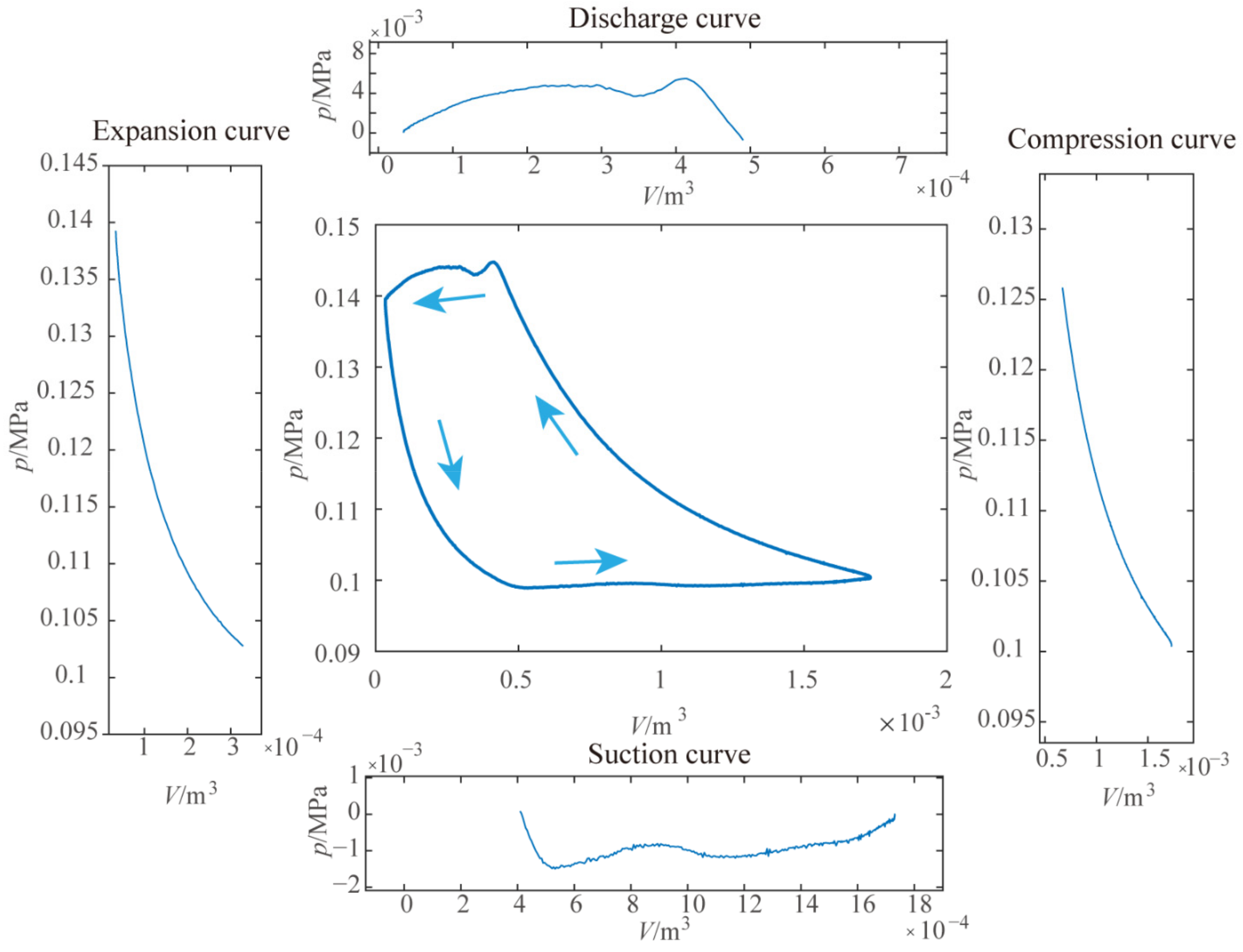
When the piston reaches the top-dead-center (TDC), a new working cycle begins. At first, the piston moves from TDC to the bottom-dead-center (BDC), and the gas remaining in the cylinder expands. Until the pressure declines to the suction pressure, the suction valves open, then the suction process begins. When the piston reaches the BDC, the suction process is over and the suction valves close, then the piston moves back to the TDC and the compression begins. Until the pressure increases to the discharge pressure, the discharge valves open, and the compression is over and the discharge process begins. At last the piston reaches the TDC, the discharge process is over and the discharge valves close, the next cycle begins. Therefore, a working cycle is composed of four processes, i.e., expansion, suction, compression, and discharge. The compressor repeats this cycle over and over again. In the meantime, the pressure in the cylinder also changes with the piston movement periodically. The pressure–volume (p–V) diagram can exactly exhibit how the dynamic pressure over a working cycle changes against the working volume. The working volume is defined as [16]:
As Figure 1 shows, the p–V diagram is a closed 2D digital diagram comprising of the four thermodynamic process curves. According to the previous description, the entire p–V diagram can be divided into four sectionalized curves, as shown in Figure 1. From Figure 1, it can be seen that the characteristics of the four sectionalized curves are different, and the influence of various faults on shape change of the curves are also different. In practice, the changes of gradients of the expansion and the compression curves and the changes of fluctuations of the discharge and suction curves are the most obvious under faulty conditions.
To capture the shape change accurately, two different feature extraction methods based on DIP were proposed according to the curve characteristics. In this study, the sectionalized curves were all saved as digital images first, and the feature extraction was also employed on these digital images. The hit-or-miss transform was applied to extract the comprehensive gradients of compression curve and expansion curve. Additionally, vertical projection transform was used to extract the fluctuation of discharge curve.
2.2. Hit-or-Miss Transform (HMT)
The sectionalized curves were saved as digital images before feature extraction. A digital image comprises pixels, which is the minimal unit with a particular location and value. By convention, the top left pixel is defined as the origin of a digital image. Therefore, digital images are matrices in essential. Taking the binary image as an example, the value of the elements in matric is either 1 or 0, and 1 means white, 0 means black. Since the binary image only have two kinds of pixels, the pixels in binary images were divided into foreground and background pixels. In this study, the white pixels were foreground pixels, in contrast, the black pixel were background pixels [17].
Hit-or-miss transform (HMT) is a morphological image processing method to detect specific shape in binary images [17]. The HMT of image I is defined as:
where is structuring element to detect shapes in the foreground, is structuring element to detect shapes in the background, is the set of the foreground pixels, and is the set of the background pixels. The equation means that finds a match in , and simultaneously, finds a match in in the same position.
In this article, three pairs of structuring elements: , and , were designed to extract features of compression curve and expansion curve. The , and are all empty sets. The , and is defined as:
The three structures were selected is due to the reason that, from the perspective of digital images, the thinned compression curve and the expansion curve only comprise the three pixel structures. After the HMT was used, the number of the three pixel structures are counted, respectively, which are , and . Then, a comprehensive gradient was calculated based on the numbers of the pixel structures:
The gradient can imply the inclination of the curve. In this article, the gradient of the compression curve and the expansion curve were extracted.
2.3. Vertical Projection Transform
As mentioned in Section 2.2, a binary image is a matrix composed of value 1 and 0. The vertical projection transform (VPT) is the operation to sum each column of the matrix. Therefore, the vertical projection of the binary image is a vector in essential, and the length of the vector is the width of the image [18].
Figure 2 presents a binary faultless discharge curve and its vertical projection. It illustrates that, the width of the binary image is 600 pixels, and in the left flat potion almost all of the vertical projections are 1. Moreover, Figure 2 indicates that the value of the vertical projection near the fluctuation of the curve is bigger than other portions, this is due to that the gradient near the fluctuation is much bigger. This means the vertical projection of the curve can reflect the fluctuations of the curve. To reduce the data dimensions, the vertical projection was divided into six parts, and the values were summed up in each portion, which was finally turned into a new feature vector including six elements.
2.4. The ANN Structure
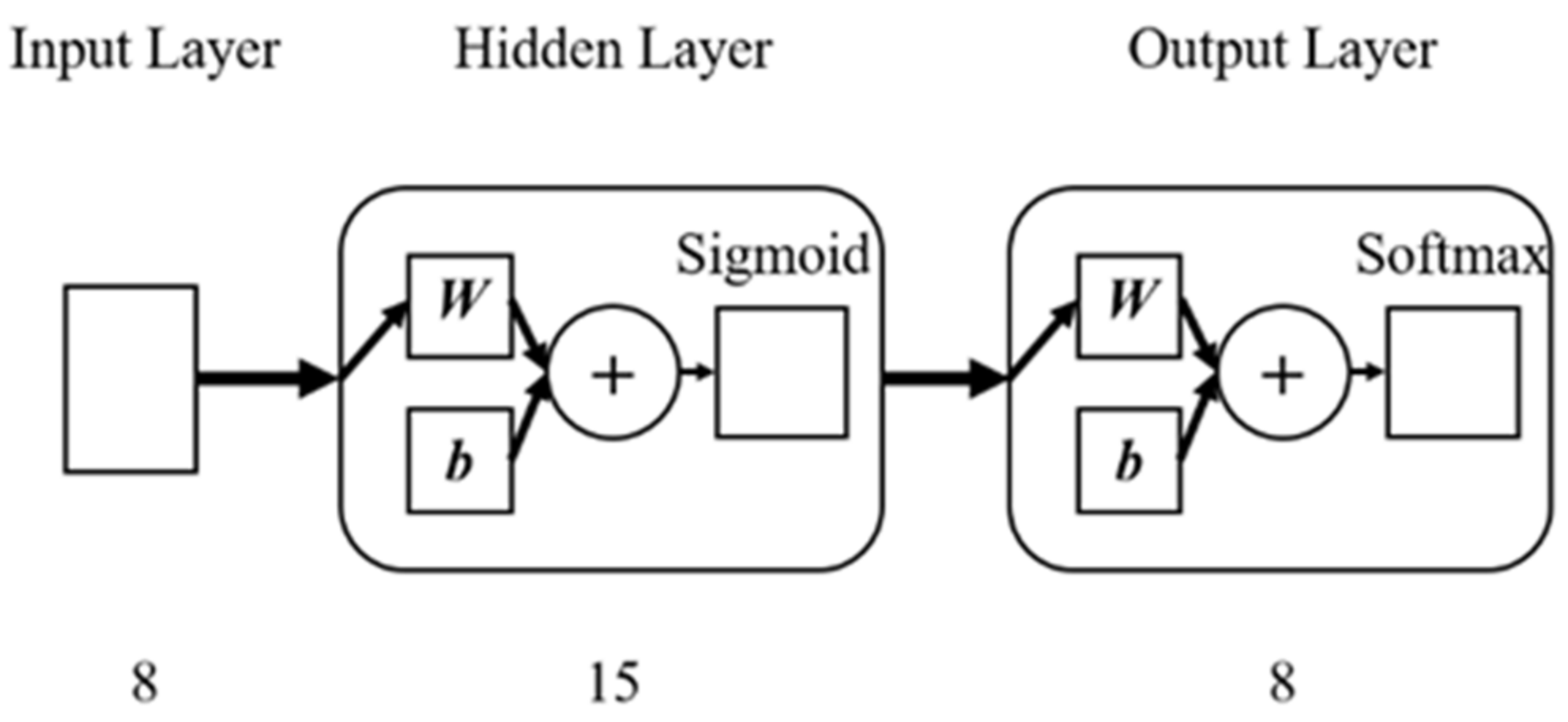
A three-layer artificial neural network (ANN) was applied to conduct fault classification in this approach as shown in Figure 3. The ANN is composed of three layers, input layer, hidden layer, and output layer. The input layer has 8 neurons corresponding to the extracted feature vector involving the comprehensive gradients, and , and the vertical projection vector . The composition of the input vector is shown in Table 1. The hidden layer has 15 neurons. The number of hidden neurons is decided by means of Manual optimization in the range of 10 to 20. Since the faultless condition and 7 faulted conditions were seeded, the output layer is a full connected layer with 8 neurons, after that is a softmax function. The softmax function is commonly exploited in output layer in multi-classification problems [19]. Further, scaled conjugate gradient was used to train this network based on cross entropy loss function.
2.5. The Proposed Fault Diagnosis Method
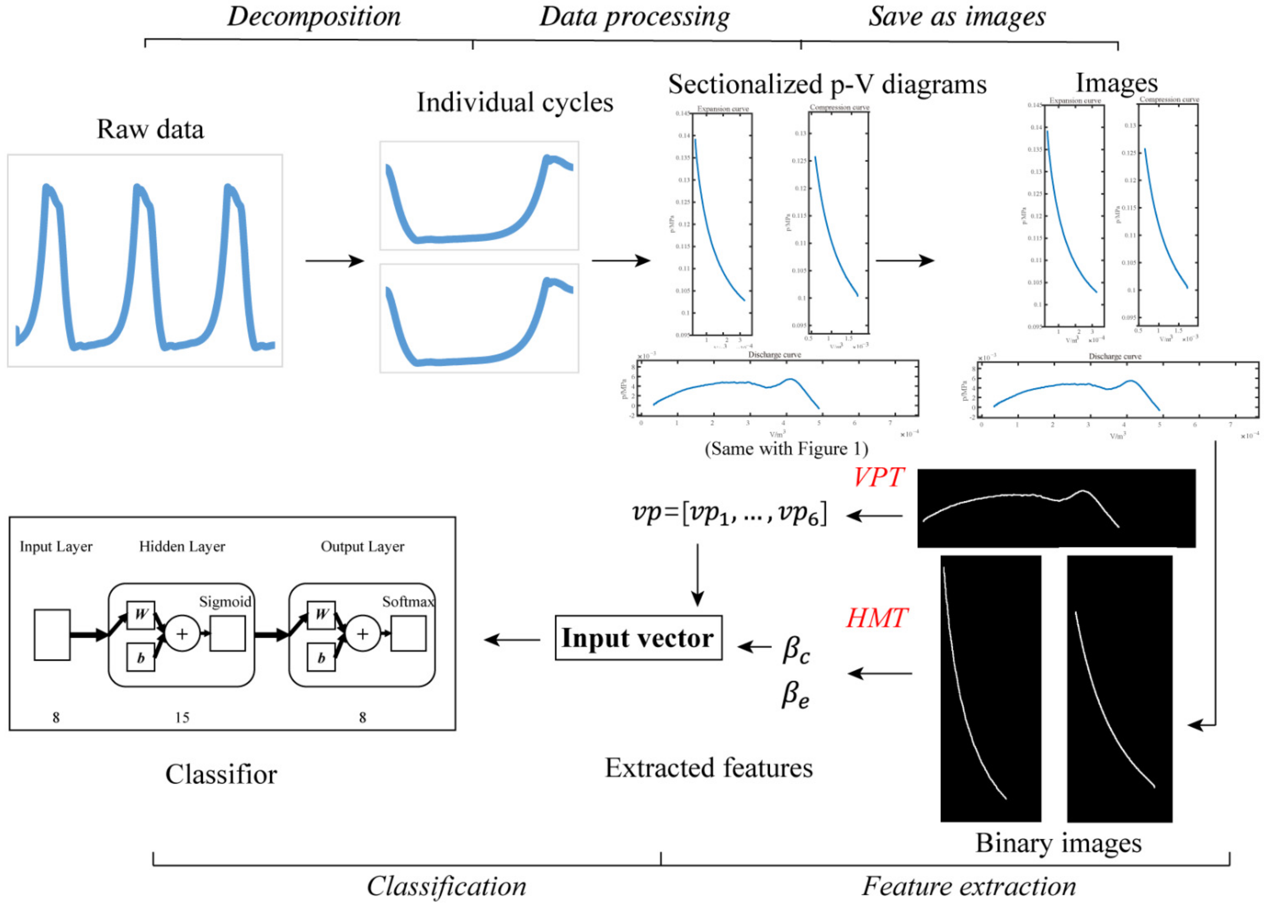
Figure 4 shows the flow block diagram of the proposed fault diagnosis method in this research. Firstly, the raw dynamic pressure data were collected from seeded fault testing. In real application, the raw data can be obtained from online condition monitoring system. Then, the raw data were decomposed into individual cycles based on the TDC signal from approach switch. The decomposition can also be based on crank position encoder in on-site application. After that, the p–V diagrams were sectionalized into four sectionalized curves including expansion curve, suction curve, compression curve, and discharge curve using MATLAB R2020a. Following that, the figures plotted in MATLAB R2020a were saved as PNG images. Then, all images were cropped to delete the axis, labels and titles, and binary processing was conducted to remove the color information. The preprocessing of the images was also conducted in MATLAB R2020a. Afterwards, HMT was applied to extract the comprehensive gradients of binary expansion curve and expansion curve, which are and , and vertical projection transform (VPT) was adopted to extract the vertical projection feature of binary discharge curve. Finally, , and were fed to the ANN classifier to obtain the fault type.
3. Seeded Fault Testing
3.1. Reciprocating Compressor Test Rig
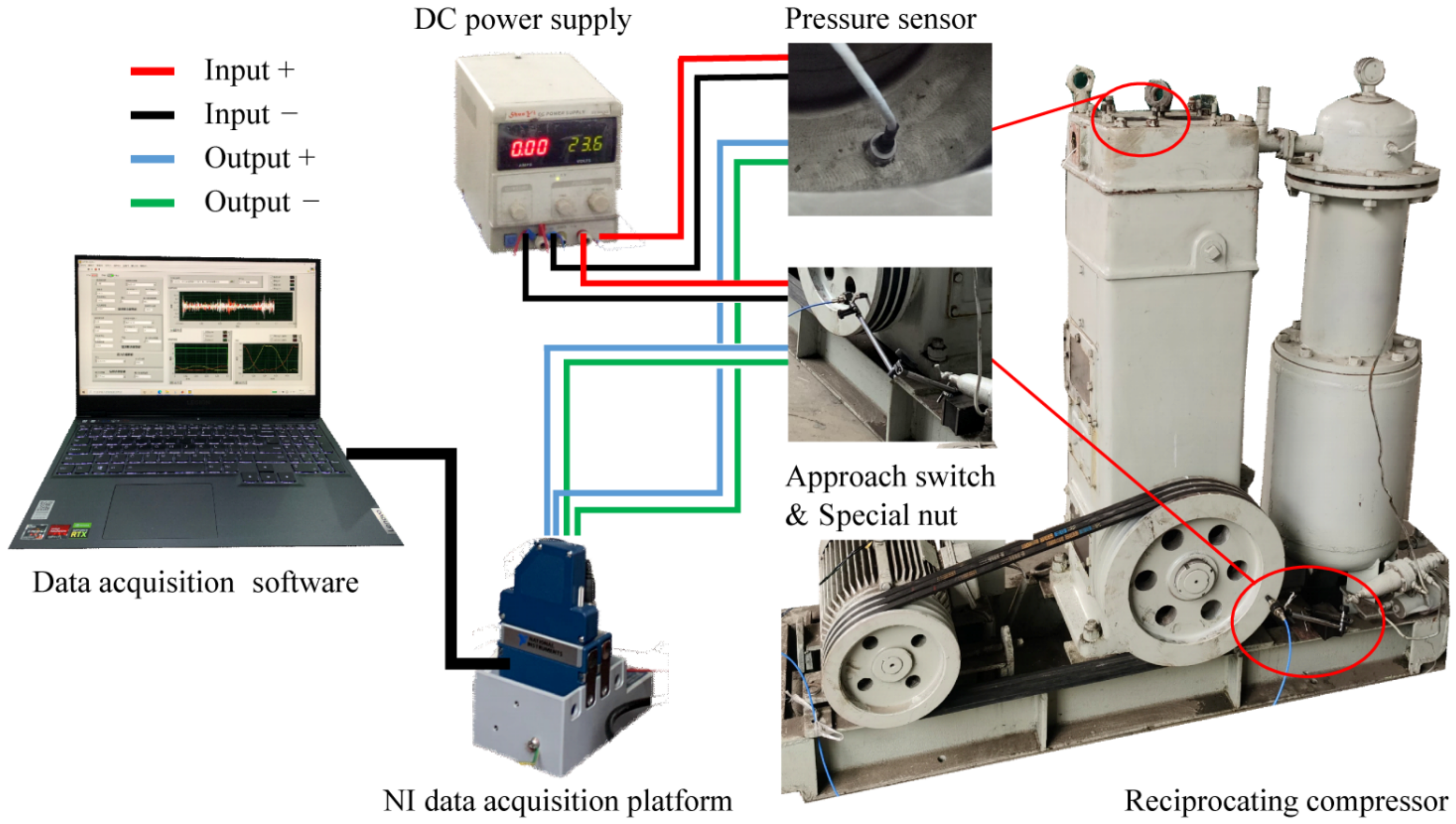
The seeded fault testing was conducted on an air RC shown in the right of Figure 5 and the parameters of it is listed in Table 2. The suction pressure is the atmosphere pressure and the discharge pressure can be adjusted by regulating opening of a valve located on the gas exhaust piping. The discharge pressure ranges from 0 to the highest pressure of 0.8 MPaG (Gauge pressure).
As Figure 5 shows, the test system is instrumented with a dynamic piezoelectric pressure sensor, an approach switch, a special nut, a direct current (DC) power supply, a NI data acquisition (DAQ) platform 9205, a laptop with a data acquisition software LabVIEW and cables for data transmission and power supply. The DC power supply was employed to provide power to sensors using the “input +” and “input –” cables. The special nut was used to identify the moment when the piston approaches the TDC. In a cycle, when the piston approaches the TDC, the special nut will pass the approach switch, then the approach switch will produce a pulse voltage signal. The time between the two adjacent pulse signals is one working cycle. In the same time, the dynamic pressures in the cylinder during a working cycle were collected by the pressure sensor. The NI DAQ platform 9205 was used to acquire the data from sensors using the “output +” and “output −” cables, and converts analog signals to digital signals, then pass the data to the software. In this study, only two channels of it were selected to conduct data collection, and the sample frequency of each channel is 10 kHz. The data acquisition software LabVIEW was employed to program hardware, collect, record, and download the data from NI DAQ 9205. With the known compressor parameters, the TDC position, and the dynamic pressures, a p–V diagram can be obtained for a cycle.
3.2. Seeded Fault Tests
To observe the changes of the operating parameters under the faultless and faulted working conditions and validate the performance of the proposed fault diagnosis method, seven common seeded faults were introduced into the reciprocating compressor test rig to obtain real faulted and faultless data. The seven seeded fault cases and the faultless case were listed in Table 3.
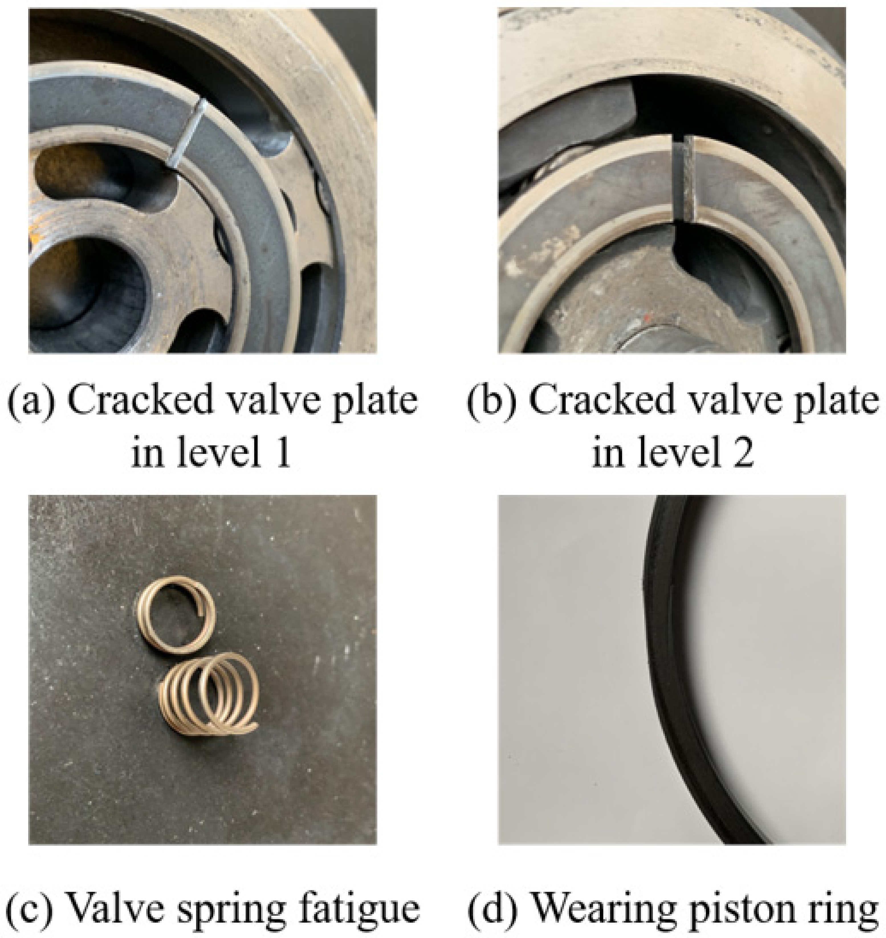
The ring valve plate may crack like a small crevice or a bigger breach due to material defects and corrosion environment. They can both increase the gas leakage through the valve, leading to the decrease of flow rate of RC. The small cracked crevice may expand to a bigger breach in on-site application. As Figure 6a shows, a small crevice was made on the discharge and suction ring valves to induce the cracked valve plate faults in level 1 in experiments (Fault 1 and 5). Additionally, in Figure 6b, a little piece of valve plate was cut off to simulate the bigger breach in the discharge and suction valve plate faults in level 2 (Fault 2 and 6). Besides, the stiff of the valve spring may degrade over time due to fatigue damage, so one spring was cut short to simulate the fatigue fault of the spring set (Fault 3 and 7), see Figure 6c. Further, the piston ring may wear gradually because of the uneven stress, which can increase the gas leakage between the piston ring and the cylinder. Figure 6d shows one side of the piston ring was scuffed to induce the wearing piston ring fault (Fault 4).
In faulted tests, the healthy components were replaced by the associated faulted components, respectively. In each faulted and faultless tests, the compressor was operating at the same suction pressure and the same regulating valve opening. Additionally, the data were sampled continuously more than 10 s in each test and were downloaded onto the laptop.
Then, MATLAB R2020a was applied to plot p–V diagrams based on the raw data. In this article, 96 groups of p–V diagrams were selected in each case; therefore, there were 768 samples in all, with eight classes. In each class, 70% of the samples were used to train the ANN, 15% of the samples were applied to do the validation, and the other 15% were used to test the performance of the ANN.
4. Results and Discussion
4.1. The Test Results
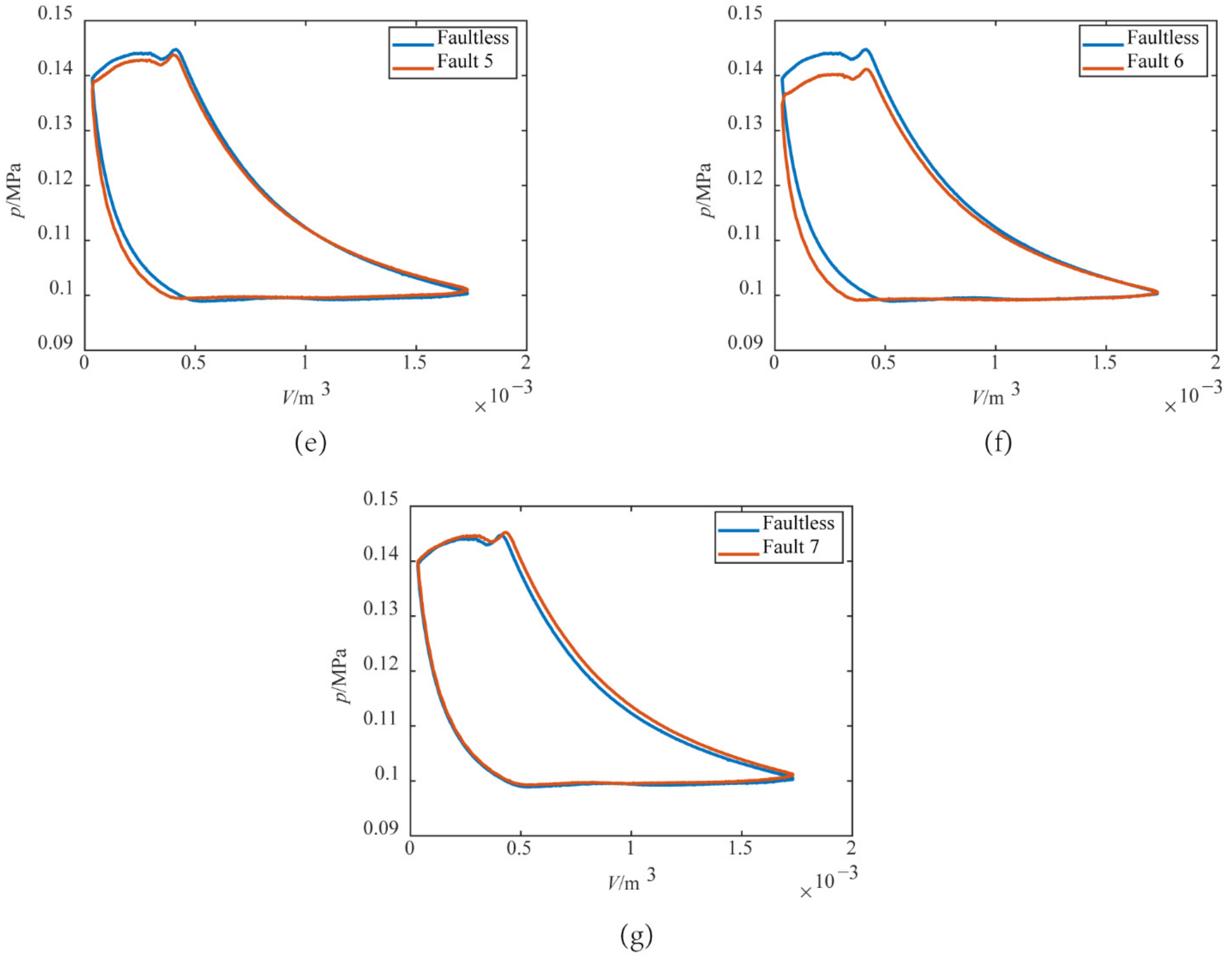
Figure 7 compares the differences of p–V diagrams of the seven faulted cases and that of the faultless case, respectively.
From Figure 7a,b, for fault 1 and fault 2, it can be seen that, the gradient of compression curve increased, and the gradient of expansion curve declined compared to those in the faultless case. This is because the gas of high pressure in the discharge chamber leaked into the cylinder through the cracked discharge valve during the compression process, which leads to the result that the pressure increased more quickly in the compression process. Moreover, the gas of high pressure also leaked into the cylinder during the expansion process, which resulted in that more high pressure gas expanded and the pressure declined more slowly. Additionally, since the gas leaking into cylinder occupied the working volume, the flow rate of the compressor dropped. With the fixed regulating valve opening, the discharge pressure went down. Besides, the discharge curve showed fluctuation at the end of discharge process. It is due to the fact that the piston speed slowed down when the piston was close to the TDC and the discharge pressure was lower than that under the faultless condition, both of which leads to a lower gas thrust. The lower gas thrust could not overcome the spring force, so the discharge valve closed in advance, whereas the compression went on and the compressed gas pushed the discharge valve to open again soon. Therefore, the quick closing and opening of the discharge valve cause the fluctuation at the end of the discharge process. The shape change of diagram of Fault 2 is more obvious compared to that of Fault 1. This is due to the fact that Fault 2 is much severer than Fault 1 and Fault 1 can develop to Fault 2 in on-site application.
In Figure 7c, the faulty and faultless diagrams almost overlapped with each other. This is because in Fault 3 the designed degradation of the spring is slight, and the fault almost cannot be reflected in p–V diagrams. This fault is corresponding to the case that incipient defects of the spring arise. If the defects develop as much severer faults, the discharge valve will open earlier and the discharge pressure will also drop.
For Fault 4, 5, and 6, Figure 7d–f illustrated that the gradient of compression curve declined and the gradient of expansion curve increased. The reason is that, during the compression and expansion processes, the gas of high pressure leaked out of the cylinder through the wearing piston ring or the cracked suction valve, respectively, both of which lead to a faster descent of pressure during the expansion process and a slower climb of pressure during the compression process. Therefore, when the compressor is single-acting, the impact of Fault 4 on the p–V diagram is similar with that of Fault 5 and 6.
Figure 7g revealed that the suction pressure in the fault 7 is higher than that under faultless condition. This is because the degradation of the spring led to the earlier opening of the suction valve. Further, the gradient of the compression curve increased, which is because the higher initial pressure made the compression proceed more quickly.
4.2. The Results of the Proposed Method
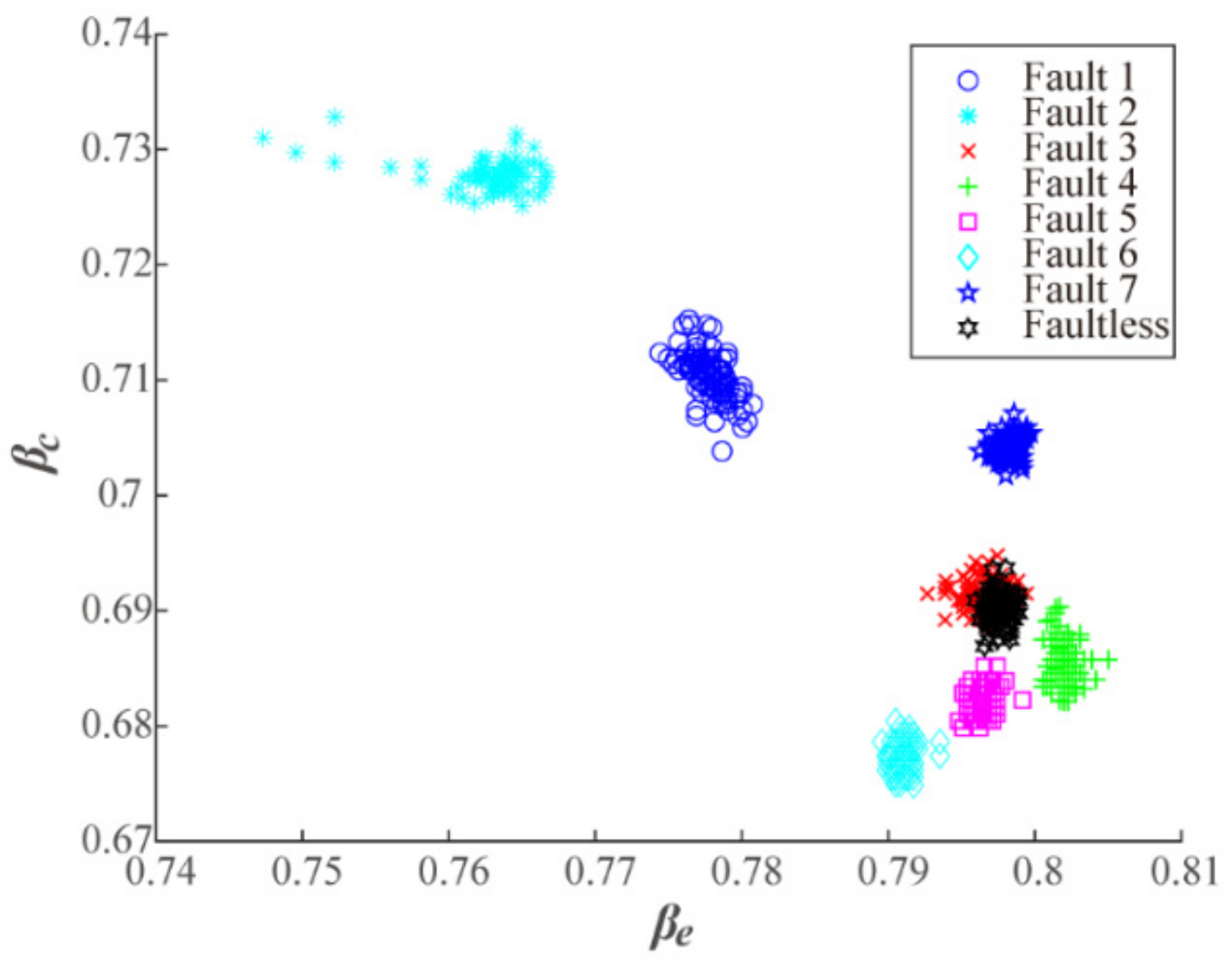
To exhibit the feature space intuitively, the distribution of the first two extracted features, and , were plotted in Figure 8. The figure showed that most of the cases can be distinguished from each other with the first two features, except Fault 3 and the faultless cases. About 60% of the feature space of samples in the case of Fault 3 overlapped the feature space of the faultless case. This can also be explained by Figure 7c. Since the two p–V diagrams almost overlapped with each other in Figure 7c, the extracted feature should also be similar. In general, however, with the help of the first two image features, the differences between different conditions already become more clear and distinguishable.
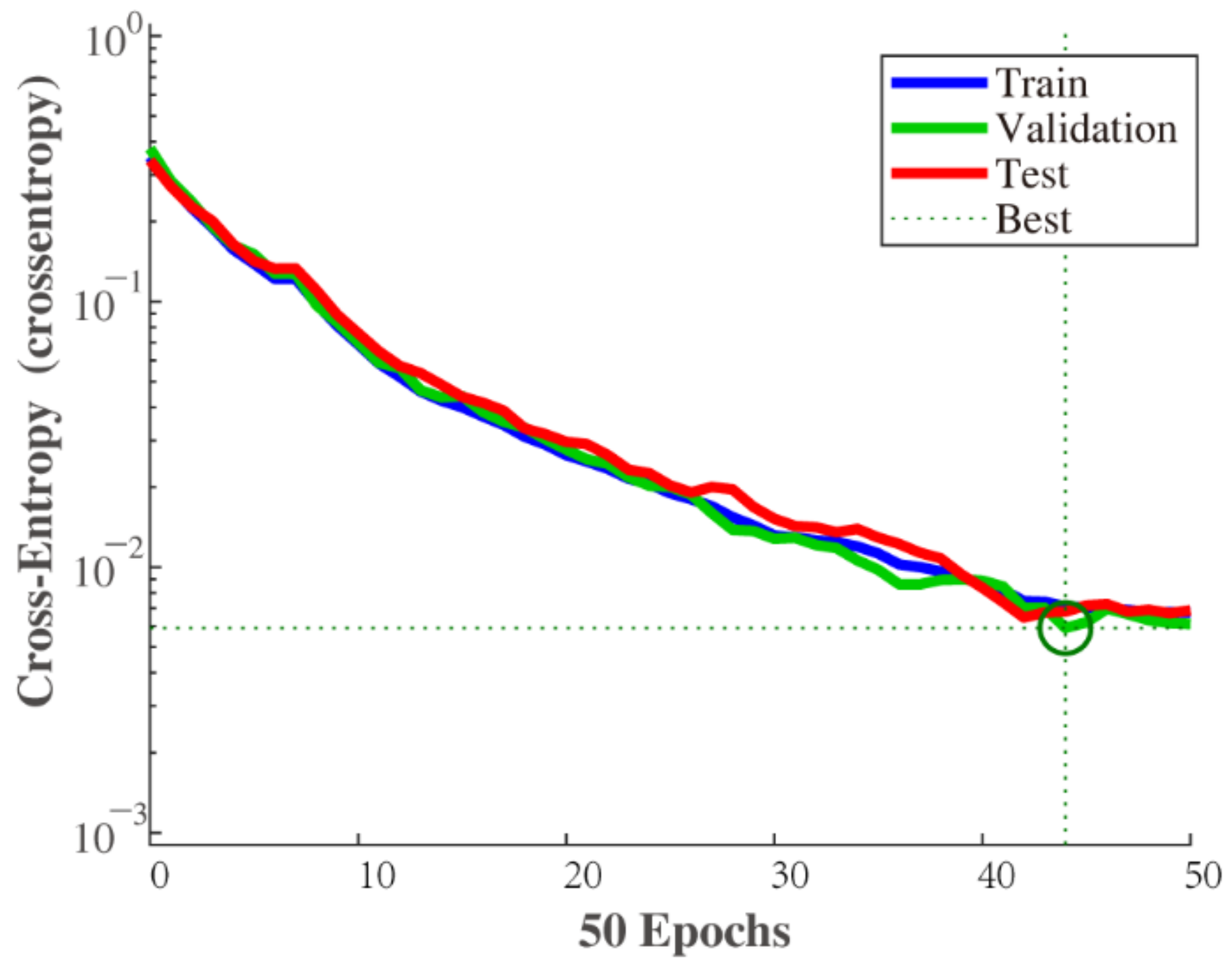
The loss curves of the model during training, validation and testing were shown in Figure 9. Figure 9 implies that the loss of the training process decreased steadily first and tend to be stable after the 40th iteration and the loss is smaller than 0.01. This suggests that the ANN model is well trained. Besides, the loss during training is similar with that during validation, which implies that the model has excellent generalization. The loss curve of the testing also proves that.
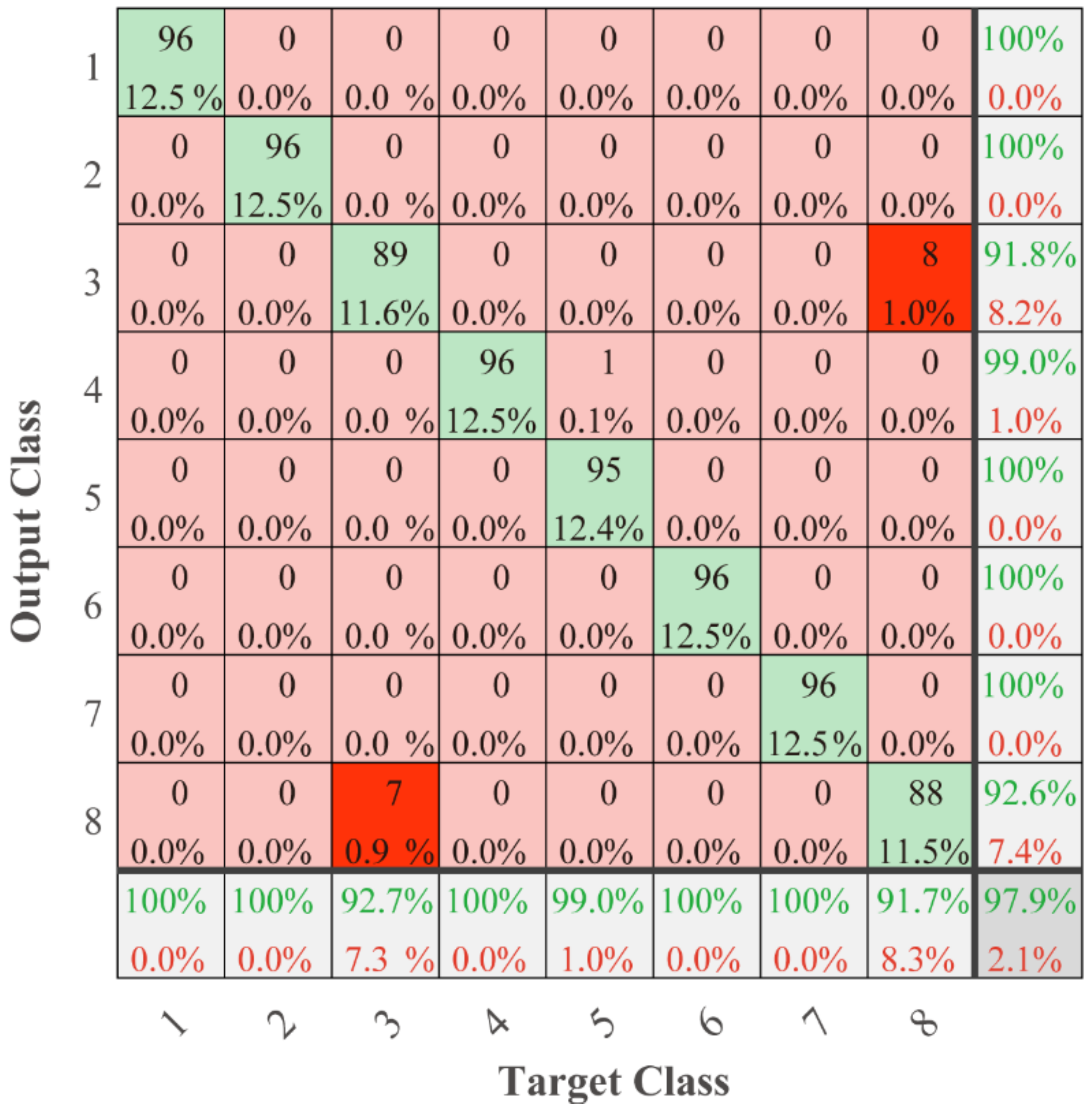
Then, the classification performance of the ANN was indicated as the confusion matrix of all samples shown in Figure 10. In Figure 10, each column represents the target class, and each row represents the predicted class. When the predicted class is consistent with the target class, the block is green; otherwise, the block is pink. Additionally, the main misclassifications were marked red in Figure 10. We can see that seven samples (7.3%) in the Fault 3 class were mistaken for the faultless class, and eight samples (8.3%) in the faultless class were mistaken for the Fault 3 class. It benefits from the vertical projection features in the input vector that the percentage of misclassification of the classes 3 and 8 not being as high as that of the feature space showed (Figure 7). This confirms that it is necessary to extract the vertical projection features from the discharge curve. In general, the entire classification accuracy of the ANN model achieved 97.9% based on the eight extracted features, even if the incipient defect cases were included, which is accurate enough in engineering applications.
To demonstrate the advantages of this method, several common machine learning algorithms were compared in this paper. The same sample set extracted by methods mentioned above was used to trained the ANN, SVM (support vector machine), and RF (random forest) models. The features extracted from raw data are mutually independent, however, CNNs are widely adopted for solving problems in which the data are related, so the raw data set was used to train the 1D CNN (convolutional neural network) model. The results were classification performance of four algorithms on validation sets by means of 5-fold cross validation, which were shown in Figure 11. The sixth results are the average of the results of the 5-fold cross validation. From Figure 11, we can see the performance of 1D CNN model based on raw data is the worst, since the dimension of the input vector for it is too high, and there were not enough samples to train a good 1D CNN model. Additionally, we can see the classification accuracy of ANN model is the best, which is over 90%. However, the classification accuracies of SVM and RF are about 83% and 60%, respectively, which proves that the superiority of the ANN algorithm is considerable.
5. Conclusions
In this paper, a novel fault diagnosis approach for RC based on p–V diagrams and image processing technologies was proposed. The raw pressure data in a working cycle of the compressor were employed to plot a p–V diagram, then the p–V diagram were decomposed into four sectionalized curves according to the working processes happened in the cylinder. Afterwards, HMT was used to extract the comprehensive gradients of compression and expansion curves, and VPT was applied to extract the vertical projection features of the discharge curve. Finally, all the features were feed to the ANN classifier to obtain the predicted class.
To validate the performance of the proposed method, a seeded fault testing was conducted on a RC test rig to collect real running data. Seven faulty cases and the healthy case were seeded in the test rig. The impacts of different faults on p–V diagrams were discussed, and the results showed that the gradients of the compression and expansion curves and the fluctuation of the discharge curve are sensitive in the faulty cases, according to the analysis of the experimental results shown in Figure 7.
Finally, the proposed method was adopted on the data from the seeded fault testing. The experimental results showed that the new method is steady during training, and has a good performance in classification, with an accuracy of 97.9%.
Author Contributions
Conceptualization, Q.L. and X.Y.; methodology, Q.L. and X.Y.; software, Q.L.; validation, Q.L. and H.M.; formal analysis, Q.L. and L.C.; investigation, Q.L.; resources, X.Y. and L.C.; data curation, Q.L.; writing—original draft preparation, Q.L.; writing—review and editing, Q.L., X.Y., L.C. and Y.S.; visualization, Q.L.; supervision, X.Y., L.C. and Y.L.; project administration, X.Y.; funding acquisition, X.Y. and Y.L. All authors have read and agreed to the published version of the manuscript.
Funding
This work was supported by the National Natural Science Foundation of China [grant numbers 52076166] and Open Foundation of State Key Laboratory of Compressor Technology (Compressor Technology Laboratory of Anhui Province), No. SKL-YSJ202111.
Conflicts of Interest
The authors declare no conflict of interest.
Nomenclature
| pressure in the cylinder, MPaG | |
| Working volume, | |
| Crank angle, degree | |
| Ratio of the crank radius to the length of the connecting rod | |
| Crank radius, m | |
| Diameter of Cylinder i, m | |
| Clearance volume, | |
| , | comprehensive gradient of compression curve and expansion curve, |
| vertical projection vector | |
| Length of the connecting rod, mm | |
| Compressor crank speed, rpm | |
| Piston stroke, mm | |
| Nominal discharge pressure, MPaG |
References
- Bloch, H.P. A Practical Guide to Compressor Technology, 2nd ed.; John Wiley & Sons, Inc.: Hoboken, NJ, USA, 2006. [Google Scholar]
- Tian, C.; Xing, Z.; Pan, X.; Wang, H. A GA-LSSVM approach for predicting and controlling in screw chiller. Proc. Inst. Mech. Eng. Part A J. Power Energy 2021, 235, 1649–1660. [Google Scholar] [CrossRef]
- Qi, G.; Zhu, Z.; Erqinhu, K.; Chen, Y.; Chai, Y.; Sun, J. Fault-diagnosis for reciprocating compressors using big data and machine learning. Simul. Model. Pract. Theory 2018, 80, 104–127. [Google Scholar] [CrossRef]
- Lv, Q.; Yu, X.; Ma, H.; Ye, J.; Wu, W.; Wang, X. Applications of Machine Learning to Reciprocating Compressor Fault Diagnosis: A Review. Processes 2021, 9, 909. [Google Scholar] [CrossRef]
- Pichler, K.; Lughofer, E.; Pichler, M.; Buchegger, T.; Klement, E.P.; Huschenbett, M. Fault detection in reciprocating compressor valves under varying load conditions. Mech. Syst. Signal Process. 2016, 70–71, 104–119. [Google Scholar] [CrossRef]
- Tran, V.T.; Althobiani, F.; Tinga, T.; Ball, A.; Niu, G. Single and combined fault diagnosis of reciprocating compressor valves using a hybrid deep belief network. Proc. Inst. Mech. Eng. Part C J. Mech. Eng. Sci. 2017, 232, 3767–3780. [Google Scholar] [CrossRef] [Green Version]
- Liu, Y.; Duan, L.; Yuan, Z.; Wang, N.; Zhao, J. An Intelligent Fault Diagnosis Method for Reciprocating Compressors Based on LMD and SDAE. Sensors 2019, 19, 1041. [Google Scholar] [CrossRef] [PubMed] [Green Version]
- Li, X.; Peng, X.; Zhang, Z.; Jia, X.; Wang, Z. A new method for nondestructive fault diagnosis of reciprocating compressor by means of strain-based p–V diagram. Mech. Syst. Signal Process. 2019, 133, 106268. [Google Scholar] [CrossRef]
- Feng, K.; Jiang, Z.; He, W.; Ma, B. A recognition and novelty detection approach based on Curvelet transform, nonlinear PCA and SVM with application to indicator diagram diagnosis. Expert Syst. Appl. 2011, 38, 12721–12729. [Google Scholar] [CrossRef]
- Wang, F.; Song, L.; Zhang, L.; Li, H. Fault Diagnosis for Reciprocating Air Compressor Valve Using P-V Indicator Diagram and SVM. In Proceedings of the 2010 Third International Symposium on Information Science and Engineering, Shanghai, China, 24–26 December 2010; pp. 255–258. [Google Scholar] [CrossRef]
- Pichler, K.; Lughofer, E.; Pichler, M.; Buchegger, T.; Klement, E.; Huschenbett, M. Detecting broken reciprocating compressor valves in the pV diagram. In Proceedings of the 2013 IEEE/ASME International Conference on Advanced Intelligent Mechatronics (AIM), Wollongong, Australia, 16 September 2013; pp. 1625–1630. [Google Scholar]
- Pichler, K.; Lughofer, E.; Pichler, M.; Buchegger, T.; Klement, E.P.; Huschenbett, M. Detecting cracks in reciprocating compressor valves using pattern recognition in the pV diagram. Pattern Anal. Appl. 2014, 18, 461–472. [Google Scholar] [CrossRef]
- Guerra, C.J.; Kolodziej, J.R. A Data-Driven Approach for Condition Monitoring of Reciprocating Compressor Valves. J. Eng. Gas Turbines Power 2014, 136, 041601. [Google Scholar] [CrossRef]
- Guerra, C.J. Condition Monitoring of Reciprocating Compressor Valves Using Analytical and Data-Driven Methodologies. Master’s Thesis, Rochester Institute of Technology, Rochester, NY, USA, 2013. [Google Scholar]
- Elhaj, M.; Gu, F.; Ball, A.; Albarbar, A.; Al-Qattan, M.; Naid, A. Numerical simulation and experimental study of a two-stage reciprocating compressor for condition monitoring. Mech. Syst. Signal Process. 2008, 22, 374–389. [Google Scholar] [CrossRef]
- Qu, Z.C. Principle of Reciprocating Compressor, 1st ed.; Xi’an Jiaotong University Press: Xi’an, China, 2019. (In Chinese) [Google Scholar]
- Gonzalez, R.C.; Woods, R.E. Digital Image Processing, 4th ed.; Pearson Education: New York, NY, USA, 2018. [Google Scholar]
- Tian, Y.; Peng, F.Y. Digital Image Processing and Analysis, 1st ed.; Huazhong University of Science & Technology Press: Wuhan, China, 2009. (In Chinese) [Google Scholar]
- Mikolov, T.; Sutskever, I.; Chen, K.; Corrado, G.; Dean, J. Distributed Representations of Words and Phrases and their Compositionality. Adv. Neural. Inf. Process. Syst. 2013, 26, 1–6. [Google Scholar]
Figure 1.
A p–V diagram.

Figure 2.
A binary discharge curve image (upper) and its vertical projection diagram (below).

Figure 3.
The structure of the ANN.

Figure 4.
The flow block diagram of the proposed method.

Figure 5.
Schematic of reciprocating compressor test rig.

Figure 6.
Faulted compressor components.

Figure 7.
Comparison of faulted and faultless diagrams: (a) Fault 1 and Faultless; (b) Fault 2 and Faultless; (c) Fault 3 and Faultless; (d) Fault 4 and Faultless; (e) Fault 5 and Faultless; (f) Fault 6 and Faultless; (g) Fault 7 and Faultless.
Figure 7.
Comparison of faulted and faultless diagrams: (a) Fault 1 and Faultless; (b) Fault 2 and Faultless; (c) Fault 3 and Faultless; (d) Fault 4 and Faultless; (e) Fault 5 and Faultless; (f) Fault 6 and Faultless; (g) Fault 7 and Faultless.


Figure 8.
Features of samples.

Figure 9.
Loss curves during training, validation and testing.

Figure 10.
Confusion matrix of all samples.

Figure 11.
Comparison of ANN, SVM, RF and 1D CNN models.


Table 1.
The composition of the input vector.
| Input Vector | Indexes |
|---|---|
| 1 | |
| 2 | |
| 3:8 |
Table 2.
Parameters of the studied compressor.
| Compressor | |
|---|---|
| The Type of the Compressor | One-Stage, Single-Acting |
| (rpm) | 625 |
| (mm) | 147 |
| (mm) | 100 |
| (MPaG) | 0–0.8 |
| (mm) | 200 |
Table 3.
Seeded fault cases.
| Seeded Faults | Cases |
|---|---|
| Cracked discharge valve plate in level 1 | Fault 1 |
| Cracked discharge valve plate in level 2 | Fault 2 |
| Broken discharge valve spring | Fault 3 |
| Wearing piston ring | Fault 4 |
| Cracked suction valve plate in level 1 | Fault 5 |
| Cracked suction valve plate in level 2 | Fault 6 |
| Broken suction valve spring | Fault 7 |
| Healthy condition | Faultless (case 8) |
Publisher’s Note: MDPI stays neutral with regard to jurisdictional claims in published maps and institutional affiliations. |
© 2022 by the authors. Licensee MDPI, Basel, Switzerland. This article is an open access article distributed under the terms and conditions of the Creative Commons Attribution (CC BY) license (https://creativecommons.org/licenses/by/4.0/).
Share and Cite
MDPI and ACS Style
Lv, Q.; Cai, L.; Yu, X.; Ma, H.; Li, Y.; Shu, Y. An Automatic Fault Diagnosis Method for the Reciprocating Compressor Based on HMT and ANN. Appl. Sci. 2022, 12, 5182. https://0-doi-org.brum.beds.ac.uk/10.3390/app12105182
AMA Style
Lv Q, Cai L, Yu X, Ma H, Li Y, Shu Y. An Automatic Fault Diagnosis Method for the Reciprocating Compressor Based on HMT and ANN. Applied Sciences. 2022; 12(10):5182. https://0-doi-org.brum.beds.ac.uk/10.3390/app12105182
Chicago/Turabian StyleLv, Qian, Liuxi Cai, Xiaoling Yu, Haihui Ma, Yun Li, and Yue Shu. 2022. "An Automatic Fault Diagnosis Method for the Reciprocating Compressor Based on HMT and ANN" Applied Sciences 12, no. 10: 5182. https://0-doi-org.brum.beds.ac.uk/10.3390/app12105182
Note that from the first issue of 2016, this journal uses article numbers instead of page numbers. See further details here.