Aerodynamic Analyses of Airfoils Using Machine Learning as an Alternative to RANS Simulation

Abstract

The accurate prediction of aerodynamic properties is an essential requirement for the design of applications that involve fluid flows, especially in the aerospace industry. The aerodynamic characteristics of fluid flows around a wing or an airfoil are usually forecasted using the numerical solution of the Reynolds-averaged Navier–Stokes equation. However, very heavy computational expenses and lengthy progression intervals are associated with this method. Advancements in computational power and efficiency throughout the present era have considerably reduced these costs; however, for many practical applications, performing numerical simulations is still a very computationally expensive and time-consuming task. The application of machine learning techniques has seen a sharp rise in various fields over recent years, including fluid dynamics, and they have proved their worth. In the present study, a famous machine learning model that is known as the back-propagation neural network was implemented for the prediction of the aerodynamic coefficients of airfoils. The most important aerodynamic properties of the coefficient of lift and the coefficient of drag were predicted by providing the model with the name, flow Reynolds number, Mach number and the angle of attack of the airfoils with respect to the incoming flows as input parameters. The dataset for the current study was obtained by performing CFD simulations using the RANS-based Spalart–Allmaras turbulence model on four different NACA series airfoils under varying aerodynamic conditions. The data that were obtained from the CFD simulations were divided into two subsets: 70% were used as training data and the remaining 30% were used as validation and testing data. The BPNN showed promising results for the prediction of the aerodynamic coefficients of airfoils under different conditions. An RMSE value of 3.57 $\times$ 10⁻⁷ was achieved for the best performance validation case with 28 epochs when there were 10 neurons in the hidden layer. The regression plot also depicted a close to perfect fit between the predicted and actual values for the regression curves.

1. Introduction

The accurate prediction of aerodynamic properties is the basic essential requirement for the design of applications that involve fluid flows, especially in the aerospace industry. The aerodynamic characteristics of fluid flows around a wing or an airfoil are usually forecasted by numerically solving Reynolds-averaged Navier–Stokes (RANS) equations. However, very heavy computational expenses and lengthy progression intervals are associated with this approach. The advancements in computational power and efficiency over the course of the present era have considerably reduced these costs; however, for many practical applications, performing numerical simulations is still a very computationally expensive and time-consuming task. The application of machine learning techniques has seen a sharp increase in various fields over recent years and they have proved their worth. Various academics and researchers have worked on the possibility of the application of deep learning techniques for the prediction of the aerodynamic characteristics of fluid flows around airfoils. Lately, both classification algorithms and regression models that have built upon machine learning methods and their application in fluid mechanics problems have become a much more relevant topic for investigation by researchers and academics. A brief literature overview of some of these studies is presented below.

Sekar et al. [1] suggested the use of an amalgamation of a deep convolutional neural network (CNN) with a deep multilayer perceptron (MLP) for the prediction of flow fields around airfoils with incompressible laminar steady-state patterns. They achieved results in two steps, in which the airfoil geometry parameters were initially extracted using CNN and were subsequently fed into the MLP model network, along with the flow Reynolds number and angle of attack of the airfoils, to obtain the required flow parameters. They were able to produce a prediction accuracy of up to 99% for training and testing cases. Duru et al. [2] proposed an encoder–decoder CNN approach for the prediction of pressure fields around an airfoil. A RANS-based CFD simulation was performed at selected Mach numbers and attack angles to forecast the pressure fields of a known airfoil, the results of which were then provided to a neural network architecture that was trained to predict pressure fields around unknown airfoil shapes. They achieved an almost 88% rate of accuracy for unseen airfoils and accelerated the speed of the simulation process using much cheaper computational resources.

Bhatnagar et al. [3] trained a shared encoding and decoding approximation that was based on a CNN model to envisage RANS flow patterns around different airfoil shapes in varying flow settings. Similar to the previous cases, they used the flow Reynolds number and attack angles of the airfoils, along with the signed distance function (SDF) of the airfoil profile, as input parameters for the proposed training algorithm. Zelong et al. [4] built a two-layer ConvNet for nonlinear problems with large scales to forecast their aerodynamic coefficients. They claimed that their proposed method was better than existing surrogate models and had the ability to enhance the accuracy of predicting the drag and lift coefficients of airfoils. They also compared the performances of ReLU and tanh activation functions in their model and found that ReLU produced a comparatively better performance in terms of the accuracy of the predicted aerodynamic coefficients.

Duraisamy et al. [5] presented a comprehensive review of the current advances in data-driven approaches for the study of turbulence problems using RANS equations. The authors pointed out that CNN-based analyses have great potential for use in turbulence modeling problems. Ling et al. [6] worked on another artificial neural network model, which was embedded with the Galilean invariance to solve RANS turbulence models. The authors claimed that their model showed significant improvements in accurate predictions compared to the generic MLP that was not embedded with invariance properties. Zhu et al. [7] investigated subsonic attached flows around an airfoil using an artificial neural network model by constructing eddy viscosity mapping. The authors claimed that this model was more efficient than the Spalart–Allmaras model in terms of achieving convergence in fewer iterations. Fahad et al. [8] employed a radial basis function neural network as a classifier to monitor corrosion inside industrial pipes and subsequently categorize its findings based on the corrosion type. The scholars trained the network using five inputs and two output neurons with a preset target MSE value of 0.0074. They achieved a very high detection accuracy rate of around 99.45%.

Ren et al. [9] worked on an adaptive control technique that was based on a radial basis function neural network (RBFNN). The coefficient of lift of an airfoil was assumed to be the response indicator and the trailing edge flap was assumed to be the actuator. By continuously changing the attack angle of the airfoil and varying the Mach number, this model could completely suppress the buffet load over an airfoil. In their work, Chang et al. [10] presented a methodology that was also built upon RBFNN for monitoring the harmonic amplitudes of observed signals in order to prevent power quality degradation in electronic power distribution systems. This method, according to the authors, provided a better accuracy with fewer sample data in comparison to the other frequently used approaches. In another work, Younis et al. [11] employed the regression model of RBFNN to predict the growth rates of fatigue cracks in the aluminum alloys of an airplane. The network was trained using two inputs and a single output neuron with a preset target MSE of 5 × 10⁻¹¹. They discovered a good correlation between the experimental and predicted data.

Ignatyey et al. [12] developed and compared the performances of two different artificial neural network architectures that used feed-forward and recurrent models to study unsteady aerodynamic features in stretched angles of attack. The training of the NNs was conducted using experimental data. They concluded that the recurrent neural network was favorable for modeling unsteady flows. Obiols-Sales et al. [13] proposed the coupling of a physical solver and a CNN to speed up the convergence of RANS simulations. The CNN model was fed with the initial CFD simulation results from the warm-up stage as inputs from the physical solver and then, after the application of the model, the predicted results from the CNN were fed back into the physical solver for final refinement. In this way, the convergence constraints were met about 7.4 times faster for steady laminar flows, as well as turbulent flows. Berenjkoub et al. [14] worked on three different artificial neural network models, which included a CNN model, a Unet model and a Resnet model, for the identification of vortex boundary layers in wake regions. They found Unet to be better for the subject task in terms of accuracy.

Li et al. [15] implemented an unsteady aerodynamic network that was built upon long- and short-term memory to predict aerodynamic and aeroelastic responses. The parameters, such as pitching angle and plunging displacement of the selected airfoil and the flow Mach number, were fed into model as inputs to obtain the lift and pitch moment coefficients as outputs. Zhang et al. [16] worked on a recurrent neural network for the identification of nonlinear aerodynamic parameters. Unsteady aerodynamic parameters that were obtained using CFD were used, along with the excitation signals, to train the network to predict the aerodynamic forces that were produced by composite sinusoidal motion. Their model was able to precisely recognize the large-amplitude nonlinear unsteady aerodynamic forces of airfoils. Singh et al. [17] developed a framework that comprised full-field inversions to model the source term in SA turbulence using a neural network. The framework was entrenched with a RANS solver to enhance the utility of the SA model in predicting the large adverse pressure deviations in flows around airfoils, both before and after the stall occurred.

Similar to the other machine learning approaches, researchers have also extensively studied the applications of back-propagation neural networks (BPNNs). Marvuglia et al. [18] applied a back-propagation neural network that was based on an ANN technique in their study to anticipate domestic energy usage roughly one hour before the electric supply was even provided to the inhabitants. They were able to predict this usage for one complete week with a mean error of 1.5%. In another study, Sihanato et al. [19] used a BPNN to project annual rainfall in different areas. Lin et al. [20] utilized a BPNN, along with an RBFNN, to curtail hydrogen usage in the fuel cell of an electric vehicle by estimating its speed. The application of the BPNN in their study helped them to correctly estimate the speed of the vehicle. Pertiwi et al. [21] employed a BPNN to predict the ratio of lift to drag coefficients at different angles of attack. They trained their model using three input parameters, namely the tip chord, winglet height and cant angle, and one output. The ratio of lift to drag coefficients was estimated with a mean squared error of 4.96 × 10⁻⁸.

Following this survey of the literature, the possibility of the application of supervised machine learning techniques in the field of aerodynamics was further explored in this study. Since much less research has been conducted on the application of back-propagation neural networks in aerodynamics, we trained a BPNN model using an aerodynamic dataset that contained varying operating conditions as the input data and the corresponding aerodynamic coefficients as the target data. The basic aim of the present study was to devise an artificial neural network architecture that can predict the most important aerodynamic characteristics, i.e., the coefficient of drag (C_D) and coefficient of lift (C_L), that are produced by airfoils under different aerodynamic conditions. The proposed BPNN was trained as a regression analysis tool to find the coefficients of lift and drag of airfoils. This study could be a step forward in the implementation of well-established machine learning techniques in solving fluid dynamics problems, in conjunction with the existing RANS-based numerical schemes.

2. Background Theory

2.1. Numerical Simulations

The purpose of performing numerical simulations was to obtain the values of the coefficients of drag and lift that were produced by different airfoils under diverse flow conditions, which could then be utilized as the required dataset for training and testing the artificial neural network that was based on the regression learning model.

The training dataset for the current study was obtained by performing CFD simulations on four different NACA series airfoils, including NACA 0012, NACA 2415, NACA 23024 and NACA 24112. The first two airfoils belong to the NACA four-digit family and the last two airfoils belong to the NACA five-digit family. The NACA 0012 airfoil is a symmetric airfoil and is one of the most frequently used and widely researched airfoils due to its lift to drag ratio [22]. Similarly, the NACA 2415 is also one of the most widely used airfoils in the unsymmetrical airfoil category. It also has applications in wind turbines for alternate energy resources [23]. The NACA 23024 and NACA 24112 are also unsymmetrical airfoils that have various applications in aeronautics and wind turbines [24].

Numerical simulations were performed on each of the selected airfoils using 10 different Reynolds numbers, in the range of 0.5 to 5 million, at a fixed Mach number of 0.5. This range of Reynolds numbers lies in the moderate regime on the low-to-high Reynolds number scale and represents the onset of turbulence to the fully turbulent boundary layer over the airfoil [25]. The Reynolds numbers that were used in our simulations were $0.5\times {10}^6, 1.0\times {10}^6,1.5\times {10}^6,2.0\times {10}^6,2.5\times {10}^6, 3.0\times {10}^6 ,3.5\times {10}^6,4.0\times {10}^6, 4.5\times {10}^6$and$5.0\times {10}^6$.

Additionally, each airfoil with each Reynolds number was numerically simulated at different angles of attacks from 0° to 20°, with increment of 2° between each case. In total, CFD simulations of 440 cases were performed under different flow conditions. A summary of these cases is presented in

Table 1. Summary of numerically simulated flow conditions.

Airfoil	R No.	Angle of Attack
NACA 0012	0.5 × 106	0	2	4	6	8	10	12	14	16	18	20
	1.0 × 106	0	2	4	6	8	10	12	14	16	18	20
	1.5 × 106	0	2	4	6	8	10	12	14	16	18	20
	2.0 × 106	0	2	4	6	8	10	12	14	16	18	20
	2.5 × 106	0	2	4	6	8	10	12	14	16	18	20
	3.0 × 106	0	2	4	6	8	10	12	14	16	18	20
	3.5 × 106	0	2	4	6	8	10	12	14	16	18	20
	4.0 × 106	0	2	4	6	8	10	12	14	16	18	20
	4.5 × 106	0	2	4	6	8	10	12	14	16	18	20
	5.0 × 106	0	2	4	6	8	10	12	14	16	18	20
NACA 2415	0.5 × 106	0	2	4	6	8	10	12	14	16	18	20
	1.0 × 106	0	2	4	6	8	10	12	14	16	18	20
	1.5 × 106	0	2	4	6	8	10	12	14	16	18	20
	2.0 × 106	0	2	4	6	8	10	12	14	16	18	20
	2.5 × 106	0	2	4	6	8	10	12	14	16	18	20
	3.0 × 106	0	2	4	6	8	10	12	14	16	18	20
	3.5 × 106	0	2	4	6	8	10	12	14	16	18	20
	4.0 × 106	0	2	4	6	8	10	12	14	16	18	20
	4.5 × 106	0	2	4	6	8	10	12	14	16	18	20
	5.0 × 106	0	2	4	6	8	10	12	14	16	18	20
NACA 23024	0.5 × 106	0	2	4	6	8	10	12	14	16	18	20
	1.0 × 106	0	2	4	6	8	10	12	14	16	18	20
	1.5 × 106	0	2	4	6	8	10	12	14	16	18	20
	2.0 × 106	0	2	4	6	8	10	12	14	16	18	20
	2.5 × 106	0	2	4	6	8	10	12	14	16	18	20
	3.0 × 106	0	2	4	6	8	10	12	14	16	18	20
	3.5 × 106	0	2	4	6	8	10	12	14	16	18	20
	4.0 × 106	0	2	4	6	8	10	12	14	16	18	20
	4.5 × 106	0	2	4	6	8	10	12	14	16	18	20
	5.0 × 106	0	2	4	6	8	10	12	14	16	18	20
NACA 24112	0.5 × 106	0	2	4	6	8	10	12	14	16	18	20
	1.0 × 106	0	2	4	6	8	10	12	14	16	18	20
	1.5 × 106	0	2	4	6	8	10	12	14	16	18	20
	2.0 × 106	0	2	4	6	8	10	12	14	16	18	20
	2.5 × 106	0	2	4	6	8	10	12	14	16	18	20
	3.0 × 106	0	2	4	6	8	10	12	14	16	18	20
	3.5 × 106	0	2	4	6	8	10	12	14	16	18	20
	4.0 × 106	0	2	4	6	8	10	12	14	16	18	20
	4.5 × 106	0	2	4	6	8	10	12	14	16	18	20
	5.0 × 106	0	2	4	6	8	10	12	14	16	18	20

.

For the numerical simulations, the commercially available CFD software package Ansys Fluent 16.0 was used. The RANS-based one-equation turbulence model Spalart–Allmaras, which is available in Fluent, was selected for the simulations. This turbulence model was specially developed for aerospace applications [26] and is commonly used in wall-bounded flow simulations. It has been proven to produce correct estimations for cases where boundary layers are subjected to adverse pressure gradients [27]. Elaborated mathematical details regarding the governing equations of the Spalart–Allmaras model, as implemented in the Fluent software package, can be found in the Fluent user guide [28]. The most common C-type flow domain was chosen for the simulations using a distance that was equivalent to 15 chord lengths between all sides of the airfoil and the domain boundaries in order to ensure the smooth dissipation of the flow effects and avoid backflow at the exit. The flow domain was resolved using unstructured grids for the computations. Inflation layers were introduced around the airfoils to achieve y+ values of less than 1 in each case that was simulated. The boundary condition at the airfoil was selected as “wall”, whereas the “velocity inlet” and “pressure outlet” boundary conditions were selected at the flow domain inlet and exit, respectively. The airfoils are shown in Figure 1 with the meshing that was created around them, along with a zoomed-in view of the inflation layers.

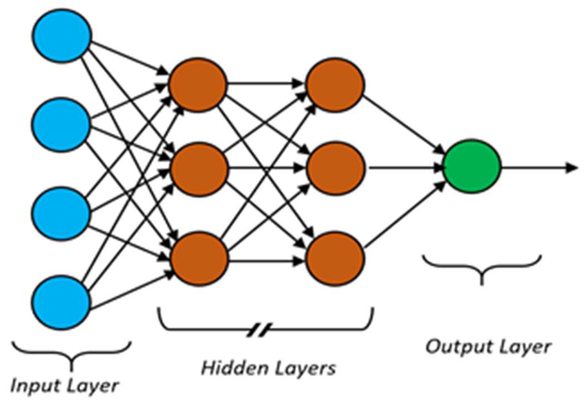
2.2. Back-Propagation Neural Network

A back-propagation neural network (BPNN) is a feed-forward type of artificial neural network that consists of three different types of layers. The three layers are known as the input layer, followed by the hidden layer(s) and, finally, the output layer. The number of hidden layers can be adjusted depending on the nature of the problem that is involved. The number of nodes, which are also known as neurons, in the input layer is selected in such a way that it matches the quantity of input features; similarly, the number of nodes or neurons in the output layer is equivalent to the number of outputs [29]. All of the processing elements, which are also known as nodes or neurons, in every layer are fully interlinked to the neurons that are in the succeeding layer through weighted connections. The inputs to the hidden layers are multiplied by the weights that are associated with the respective neurons and are then added together by the hidden layer to produce a summed output. This summed output is then passed through an activation function, such as sigmoid, tan-sigmoid or threshold functions [30]. Due to the simplicity, efficient performance and ease of implementation, it is one of the most extensively used neural networks. The general architecture of a BPNN with one output is shown in Figure 2.

Our BPNN was built upon a simplified Widrow–Hoff learning rule, which is also known as the generalized delta rule, and used a supervised learning technique. [31]. For training, we used the gradient descent method [32], which was applied by adopting the following procedure:

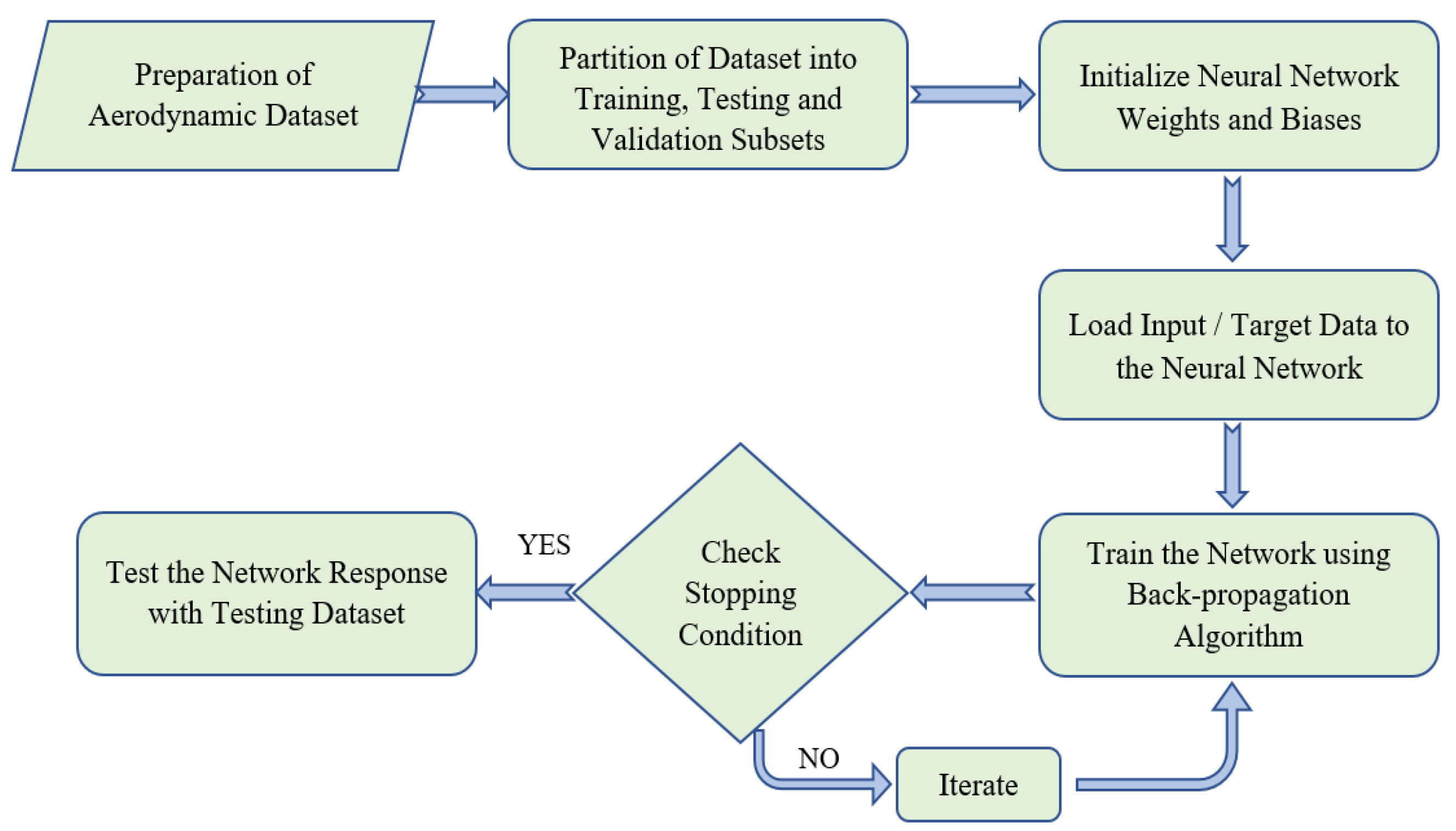
• Initialize all weights $w_{ij}^{\left[l\right]}$ and biases $b_j^{\left[l\right]}$ by assigning random values (l = layer number, i. = 1 to N and j = 1 to M);
• Feed the training dataset and output dataset into the artificial neural network and then compute the output of each layer using Equation (1):

  $$y_{jp}^{\left[lC1\right]}=f\left({{\displaystyle \sum }}_{i=1}^{N1}{w}_{ij}^{\left[l+1\right]}{y}_{ip}^{\left[l\right]}+b_j^{\left[l+1\right]}\right)$$

  (1)
• Compute the error term at the output of each layer using Equation (2):

  $$er{r}_{jp}^{\left[L\right]}=f^{\prime }\left(y_{jp}^{\left[L\right]}\right)\left(d_p-y_{jp}^{\left[L\right]}\right)$$

  (2)

  in the ith hidden layer (i = L-1, L-2, … 1)

  $$er{r}_{jp}^{\left[l\right]}=f^{\prime }\left(y_j^{\left[l\right]}\right){{\displaystyle \sum }}_{k=1}^{N_{l+1}}er{r}_{kp}^{l+1}{w}_{jk}^{l+1}$$

  (3)
• Compute the changes in weights and biases between the input and output layers using Equations (4) and (5):

  $$b_{ij}^{\left[l\right]}\left(n+1\right)=b_i^{\left[l\right]}\left(n\right)+ŋ.er{r}_{jp}^{\left[l\right]}$$

  (4)

  $$w_{ij}^{\left[l\right]}\left(n+1\right)=w_{ij}^{\left[l\right]}\left(n\right)+ŋ.er{r}_{jp}^{\left[l\right]}.y_{ip}^{\left[l-1\right]}$$

  (5)
  It can be seen that the error term was back-propagated into the neurons of the previous layer while calculating the changes in the weights and biases;
• Repeat Steps 2 to 5 until the error term falls below the minimum specified error criteria;
• The sigmoid activation function that was used in the present study was given by Equation (6):

  $$f\left(x\right)= 1/(1+e^{-x})$$

  (6)

3. Proposed Methodology

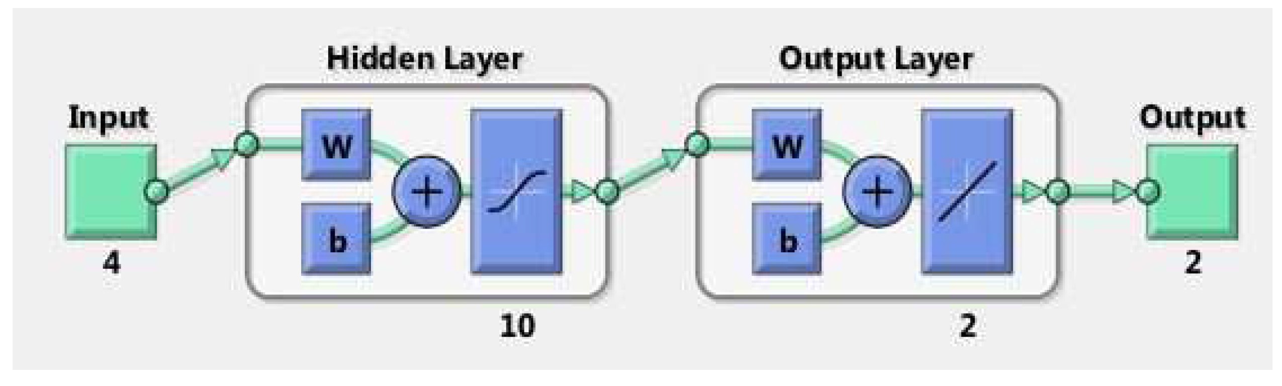
3.1. Architecture of the BPNN for the Prediction of Aerodynamic Coefficients

The basic building blocks of the proposed methodology can be seen in Figure 3. The BPNN was used as a regression analysis tool to find the coefficients of lift and drag of the airfoils. First of all, the dataset that consisted of the 440 cases that were used in this study was obtained from performing numerical simulations in the Ansys Fluent software using the RANS-based Spalart–Allmaras turbulence model on four different NACA series airfoils, including NACA 0012, NACA 2415, NACA 23024 and NACA 24112. Each of the selected airfoils was simulated with 10 different Reynolds numbers in the range of 0.5 to 5 million.

The dataset that was collected from the numerical simulations contained four input parameters, namely, airfoil name, flow Reynolds number, Mach number and airfoil angle of attack, whereas the two output parameters were coefficient of drag (C_D) and coefficient of lift (C_L). The dataset was then divided into two subsets: 70% of the data were used as training data for the network, while the other 30% were reserved for testing and validation. The neural network was then trained using the back-propagation algorithm on the training dataset. The training was continued until the achievement of the stopping criteria, after which the network response was checked using the testing subset. The stopping criteria were set to be attained when the best validation performance was achieved, i.e., when the validation error reached its minimum value.

The architecture of the BPNN that was used in this study, with four input parameters, ten neurons in the hidden layer (best performance case) and two outputs, is shown in Figure 4.

3.2. Performance Evaluation Metrics

The following statistical measures were used as performance metrics to assess the performance of the supervised machine learning method that was used in this work to forecast the aerodynamic characteristics of the airfoils:

• Root mean squared error (RMSE), which represents the error rate using the square root of the mean squared error [33]. The lower the value of RMSE, the better the accuracy of the regression model [34]. It was calculated using the expression that is given in Equation (7):

  $$RMSE=\sqrt{\frac{1}{n}{\displaystyle \sum }_{i=1}^n{\left|P_i-M_i\right|}^2}$$

  (7)
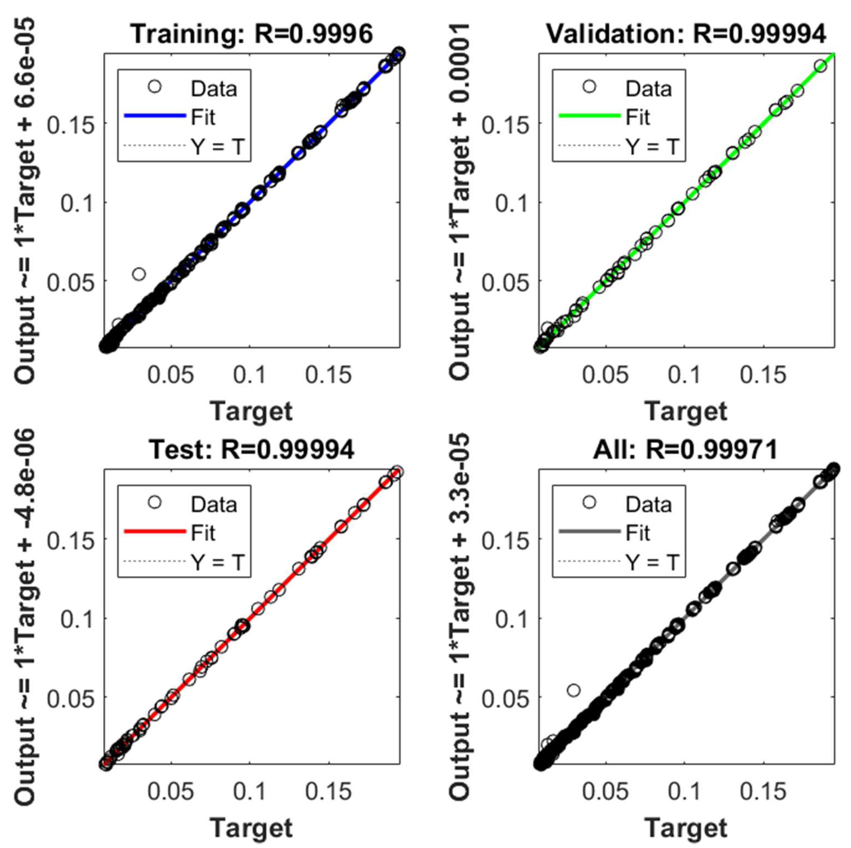
• Pearson correlation coefficient (R), which is a key factor in regression analysis that signifies the correlation between the forecasted results and the real outputs. Its value ranges from −1 to +1. The accuracy of a regression model is considered to be the best when the absolute value of R is equal or close to 1 [35]. It was calculated using the relationship that is given in Equation (8):

  $$R=\sqrt{1-\frac{{\displaystyle \sum }{\left(M_i-P_i\right)}^2}{{\displaystyle \sum }{\left(M_i-{\overline{M}}_l\right)}^2}}$$

  (8)

  where n denotes the number of data points in the testing subset, $P_i \mathrm{and} M_i$ are the predicted and measured values for the ith aerodynamic coefficient and ${\overline{M}}_l$ is the mean of all measured values for the aerodynamic coefficients.

4. Results and Discussions

The BPNN was trained in MATLAB using a diverse number of nodes or neurons in the hidden layer to obtain the best root mean squared error (RMSE) value. The results that were obtained with the varying numbers of neurons in the hidden layer are summarized in

Table 2. Summary of results using varying numbers of neurons in the hidden layer.

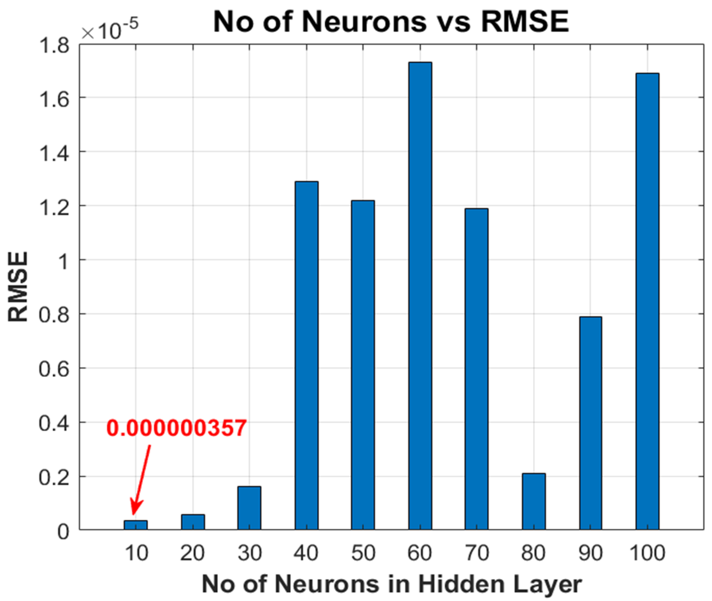
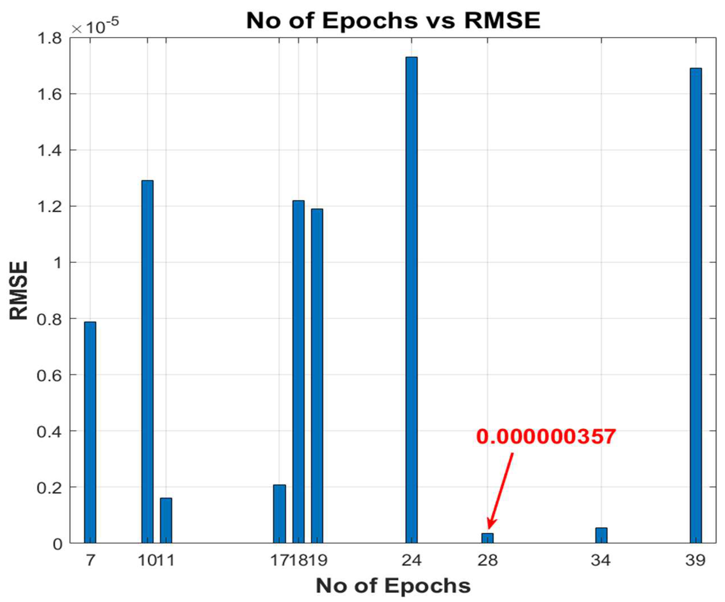
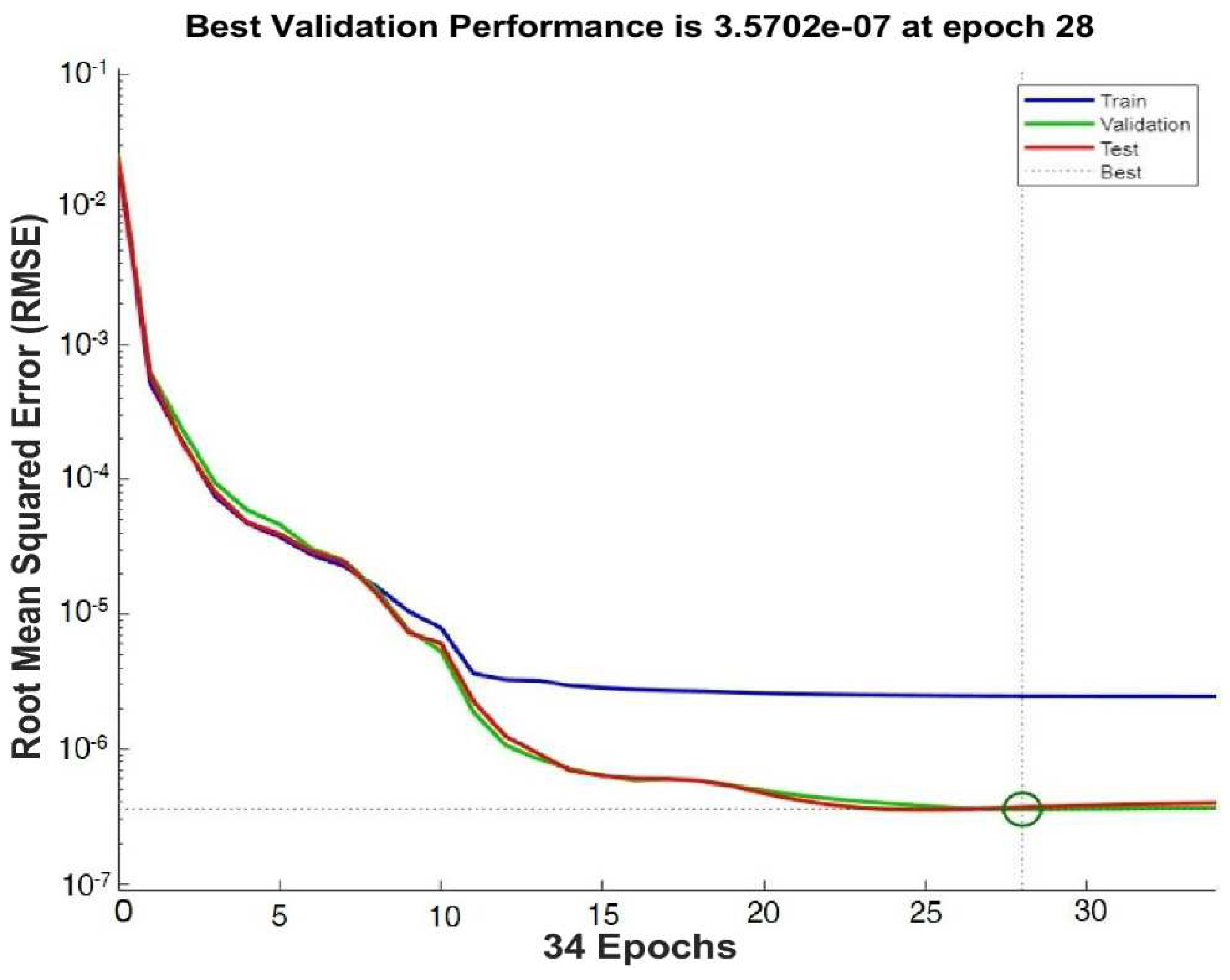
S No.	No. of Neurons	RMSE ×10−7)	No. of Epochs	Corr Coeff for Training	Corr Coeff for Validation	Corr Coeff for Testing	Corr Coeff Overall
1	10	3.57	28	0.9996	0.99994	0.99994	0.99971
2	20	5.61	34	0.99969	0.9999	0.99983	0.99974
3	30	16.2	11	0.99967	0.99976	0.99992	0.99972
4	40	129	10	0.99998	0.99805	0.99988	0.99966
5	50	122	18	0.99999	0.99761	0.99984	0.99968
6	60	173	24	0.99993	0.99669	0.99855	0.99929
7	70	119	19	1	0.99809	0.99965	0.99968
8	80	20.8	17	0.99999	0.99975	0.99816	0.99967
9	90	78.9	7	0.99984	0.99875	0.99931	0.99959
10	100	169	39	1	0.9969	0.99942	0.9995

with their respective RMSE values.

It can be seen that the best RMSE value was attained when the number of neurons in the hidden layer was 10, with RMSE value of $3.57\times {10}^{-7}$ for the validation case with 28 epochs. The correlation values (R) were very close to 1 for all of the training, validation and testing cases, which was an indication of the high accuracy of the predicted values. It is also evident from the table that the RMSE was sensitive to the number of neurons in the hidden layer, although the correlation value (R) did not show any visible variations with changes in the number of neurons in the hidden layer.

Figure 5 illustrates the association between the number of neurons in hidden layer and the RMSE value. It is evident that the minimum value of $3.57\times {10}^{-7}$ for RMSE was achieved with 10 neurons in the hidden layer. The RMSE value was sensitive to the number of neurons; however, it did not show a continuous trend or an established relationship. Initially, when the number of neurons increased from 10 to 40, the value of RMSE also increased, after which it decreased as the number of neurons increased to 50. The RMSE again increased when the number of neurons further increased to 60; however, on increasing the number of neurons further, the RMSE started to decrease until the number of neurons reached 80 in the hidden layer, after which the RMSE started to increase again until the end of the experiment.

The number of epochs vs. RMSE plot is presented in Figure 6. The network was trained with different numbers of neurons in the hidden layer. In each case, the training was continued until the best RMSE value was achieved, irrespective of the number of epochs that it took to achieve the best RMSE value. In each of the training sessions, the RMSE varied with the number of epochs. For the best case, the number of epochs was 28 with an RMSE value of $3.57\times {10}^{-7}$. Depending on the number of neurons in the hidden layer, the number of epochs varied to achieve the desired output.

A performance plot of the RMSE value and the number of epochs vs. the network response for the training, testing and validation datasets is depicted in Figure 7. The figure shows that the RMSE value was relatively high at the start of the training and gradually reduced as the training progressed. After 28 epochs, the RMSE value became constant at 3.57 $\times$ 10⁻⁷ and did not fall any further. This performance plot of RMSE vs. the number of epochs represents for the best RMSE case only. It can be seen that the RMSE values for the training data are relatively large compared to the testing and validation data, which was attributed to the limited number of training data points (440 cases) that was used in the present work [36].

A regression plot for the training, testing and validation subsets (for the best RMSE case) is depicted in Figure 8. It can be observed that the values of R were very close to 1 in all instances, which indicated a very high correlation between the predicted and actual target values. This means that a high accuracy of predicted values was achieved using this trained model. The training of the BPNN model was performed using historical data. Similarly, the validation was also performed using historical data to create a reliable model with good forecasting capabilities. The graph shows the good correlation between the target and forecasted values; additionally, practically all of the data points fall on the regression line. This figure also includes the output equations for all subsets, which illustrate the links between the target and forecasted values.

The results showed that the back-propagation neural network (BPNN) that was trained in this study could predict aerodynamic coefficients with a higher accuracy and lower number of prediction errors in the results compared to existing models. However, it should be noted that machine learning techniques are data-hungry algorithms, which require large datasets for proper training. The more data, the better the performance of the model. In the present study, the BPNN model was trained using a dataset of 440 simulation cases, which could have been a potential limitation on the performance of the model. Therefore, training this model using more data that have been obtained from further CFD simulations of different types of airfoils under numerous settings would help to increase its reliability. The model could then be utilized for the prediction of the aerodynamic coefficients of lift and drag for unseen airfoils under various conditions.

5. Conclusions

In this study, the performance of a BPNN model was evaluated in terms of its ability to predict the important aerodynamic coefficients of lift and drag of airfoils. Aerodynamic data that were attained by performing numerical simulations of 440 cases were used for the training, validation and testing of the BPNN model. It can be summarized that the BPNN showed promising results for the prediction of the aerodynamic coefficients of airfoils under various conditions. The RMSE for the best performance validation case was 3.57 $\times$ 10⁻⁷ with 10 neurons in the hidden layer and 28 epochs. The regression plots also depicted a close to perfect fit between the predicted and actual values for the regression curves.

This study could be extended in the future to examine other regression algorithms, such as radial basis function neural networks (RBFNNs), support vector regression (SVR), etc., and evaluate the performance of each algorithm in comparison to each other in order to obtain the best model for aerodynamic data prediction.

References

- Sekar, V.; Khoo, B.C. Fast flow field prediction over airfoils using deep learning approach. Phys. Fluids 2019, 31, 057103. [Google Scholar] [CrossRef]
- Duru, C.; Alemdar, H.; Baran, U. CNNFOIL: Convolutional encoder decoder modeling for pressure fields around airfoils. Neural Comput. Appl. 2021, 33, 6835–6849. [Google Scholar] [CrossRef]
- Bhatnagar, S.; Afshar, Y.; Pan, S.; Duraisamy, K.; Kaushik, S. Prediction of aerodynamic flow fields using convolutional neural networks. Comput. Mech. 2019, 64, 525–545. [Google Scholar] [CrossRef] [Green Version]
- Yuan, Z.; Wang, Y.; Qiu, Y.; Bai, J.; Chen, G. Aerodynamic Coefficient Prediction of Airfoils with Convolutional Neural Network. In Proceedings of the 2018 Asia-Pacific International Symposium on Aerospace Technology (APISAT 2018), Chengdu, China, 16–18 October 2018; Zhang, X., Ed.; Springer: Singapore, 2019; Volume 459, pp. 34–46. [Google Scholar] [CrossRef]
- Duraisamy, K.; Iaccarino, G.; Xiao, H. Turbulence Modeling in the Age of Data. Annu. Rev. Fluid Mech. 2019, 51, 357–377. [Google Scholar] [CrossRef] [Green Version]
- Ling, J.; Kurzawski, A.; Templeton, J. Reynolds averaged turbulence modelling using deep neural networks with embedded invariance. J. Fluid Mech. 2016, 807, 155–166. [Google Scholar] [CrossRef]
- Zhu, L.; Zhang, W.; Kou, J.; Liu, Y. Machine learning methods for turbulence modeling in subsonic flows around airfoils. Phys. Fluids 2019, 31, 015105. [Google Scholar] [CrossRef]
- Fahad, M.; Kamal, K.; Zafar, T.; Qayyum, R.; Tariq, S.; Khan, K. Corrosion detection in industrial pipes using guided acoustics and radial basis function neural network. In Proceedings of the 2017 International Conference on Robotics and Automation Sciences (ICRAS), Hong Kong, 26–29 August 2017; pp. 129–133. [Google Scholar] [CrossRef]
- Ren, K.; Chen, Y.; Gao, C.; Zhang, W. Adaptive control of transonic buffet flows over an airfoil. Phys. Fluids 2020, 32, 096106. [Google Scholar] [CrossRef]
- Chang, G.W.; Chen, C.-I.; Teng, Y.-F. Radial-Basis-Function-Based Neural Network for Harmonic Detection. IEEE Trans. Ind. Electron. 2010, 57, 2171–2179. [Google Scholar] [CrossRef]
- Bin Younis, H.; Kamal, K.; Sheikh, M.F.; Hamza, A.; Zafar, T. Prediction of fatigue crack growth rate in aircraft aluminum alloys using radial basis function neural network. In Proceedings of the 2018 Tenth International Conference on Advanced Computational Intelligence (ICACI), Xiamen, China, 29–31 March 2018; pp. 825–830. [Google Scholar] [CrossRef]
- Ignatyev, D.I.; Khrabrov, A.N. Neural network modeling of unsteady aerodynamic characteristics at high angles of attack. Aerosp. Sci. Technol. 2015, 41, 106–115. [Google Scholar] [CrossRef]
- Obiols-Sales, O.; Vishnu, A.; Malaya, N.; Chandramowliswharan, A. CFDNet: A deep learning-based accelerator for fluid simulations. In Proceedings of the 34th ACM International Conference on Supercomputing, Barcelona, Spain, 29 June–2 July 2020; p. 3. [Google Scholar] [CrossRef]
- Berenjkoub, M.; Chen, G.; Gunther, T. Vortex Boundary Identification using Convolutional Neural Network. In Proceedings of the 2020 IEEE Visualization Conference (VIS), Salt Lake City, UT, USA, 25–30 October 2020; pp. 261–265. [Google Scholar] [CrossRef]
- Li, K.; Kou, J.; Zhang, W. Deep neural network for unsteady aerodynamic and aeroelastic modeling across multiple Mach numbers. Nonlinear Dyn. 2019, 96, 2157–2177. [Google Scholar] [CrossRef]
- Han, J.; Zhang, B.; Zhang, T.; Ma, R. Unsteady aerodynamic identification based on recurrent neural networks. J. Vibroeng. 2020, 23, 449–458. [Google Scholar] [CrossRef]
- Singh, A.P.; Medida, S.; Duraisamy, K. Machine-Learning-Augmented Predictive Modeling of Turbulent Separated Flows over Airfoils. AIAA J. 2017, 55, 2215–2227. [Google Scholar] [CrossRef]
- Marvuglia, A.; Messineo, A. Using Recurrent Artificial Neural Networks to Forecast Household Electricity Consumption. Energy Procedia 2012, 14, 45–55. [Google Scholar] [CrossRef] [Green Version]
- Sihananto, A.N.; Mahmudy, W.F. Rainfall Forecasting Using Backpropagation Neural Network. J. Inf. Technol. Comput. Sci. 2016, 2, 66–76. [Google Scholar] [CrossRef] [Green Version]
- Lin, X.; Wang, Z.; Wu, J. Energy management strategy based on velocity prediction using back propagation neural network for a plug-in fuel cell electric vehicle. Int. J. Energy Res. 2021, 45, 2629–2643. [Google Scholar] [CrossRef]
- Pertiwi, F.D.; Wahjudi, A. Numerical Study of Blended Winglet Geometry Variations on Unmanned Aerial Vehicle Aerodynamic Performance. Int. J. Mech. Eng. Sci. 2022, 6, 1. [Google Scholar] [CrossRef]
- Michos, A.; Bergeles, G.; Athanassiadis, N. Aerodynamic Characteristics of NACA 0012 Airfoil in Relation to Wind Generators. Wind Eng. 1983, 7, 247–262. [Google Scholar]
- Yildiz, F.; Turkmen, A.C.; Celik, C.; Sarac, H.I. Pitch Angle Analysis of NACA 2415 Airfoil. In Proceedings of the World Congress on Engineering, London, UK, 1–3 July 2015; p. 5. [Google Scholar]
- Kumar, B.S.A.; Manjunath, S.; Ganganna, R. Computational Investigation of Flow Separation over Naca 23024 Airfoil at 6 Million Free Stream Reynolds Number. Int. J. Sci. Technol. Soc. 2015, 3, 315. [Google Scholar] [CrossRef] [Green Version]
- Wang, S.; Zhou, Y.; Alam, M.; Yang, H. Turbulent intensity and Reynolds number effects on an airfoil at low Reynolds numbers. Phys. Fluids 2014, 26, 115107. [Google Scholar] [CrossRef]
- Spalart, P.R.; Allmaras, S.R. A one-equation turbulence model for aerodynamic flows. In Proceedings of the 30th Aerospace Sciences Meeting and Exhibit, Reno, NV, USA, 6–9 January 1992. [Google Scholar] [CrossRef]
- Ahmed, S.; Malik, A.; Parvez, K. RANS Predictions of Junction Flow with Localized Suction. In Proceedings of the 2018 IEEE International Conference on Aerospace Electronics and Remote Sensing Technology (ICARES), Bali, Indonesia, 20–21 September 2018; pp. 1–7. [Google Scholar] [CrossRef]
- Fluent Inc. FLUENT 6.3 User’s Guide; Fluent Inc.: Lebanon, NH, USA, 2006. [Google Scholar]
- Kamal, K.; Qayyum, R.; Mathavan, S.; Zafar, T. Wood defects classification using laws texture energy measures and supervised learning approach. Adv. Eng. Inform. 2017, 34, 125–135. [Google Scholar] [CrossRef]
- Thegazy, T.; Fazio, P.; Moselhi, O. Developing Practical Neural Network Applications Using Back-Propagation. Comput.-Aided Civ. Infrastruct. Eng. 1994, 9, 145–159. [Google Scholar] [CrossRef]
- Puig-Arnavat, M.; Bruno, J.C. Artificial Neural Networks for Thermochemical Conversion of Biomass. In Recent Advances in Thermo-Chemical Conversion of Biomass; Elsevier: Amsterdam, The Netherlands, 2015; pp. 133–156. [Google Scholar] [CrossRef] [Green Version]
- Abuzneid, M.A.; Mahmood, A. Enhanced Human Face Recognition Using LBPH Descriptor, Multi-KNN, and Back-Propagation Neural Network. IEEE Access 2018, 6, 20641–20651. [Google Scholar] [CrossRef]
- Le, T.-H.; Nguyen, H.-L.; Pham, B.; Nguyen, M.; Pham, C.-T.; Nguyen, N.-L.; Le, T.-T.; Ly, H.-B. Artificial Intelligence-Based Model for the Prediction of Dynamic Modulus of Stone Mastic Asphalt. Appl. Sci. 2020, 10, 5242. [Google Scholar] [CrossRef]
- Ly, H.-B.; Pham, B.T. Prediction of Shear Strength of Soil Using Direct Shear Test and Support Vector Machine Model. Open Constr. Build. Technol. J. 2020, 14, 41–50. [Google Scholar] [CrossRef]
- Moriasi, D.N.; Gitau, M.W.; Pai, N.; Daggupati, P. Hydrologic and Water Quality Models: Performance Measures and Evaluation Criteria. Trans. ASABE 2015, 58, 1763–1785. [Google Scholar] [CrossRef] [Green Version]
- Alzubaidi, L.; Zhang, J.; Humaidi, A.J.; Al-Dujaili, A.; Duan, Y.; Al-Shamma, O.; Santamaría, J.; Fadhel, M.A.; Al-Amidie, M.; Farhan, L. Review of deep learning: Concepts, CNN architectures, challenges, applications, future directions. J. Big Data 2021, 8, 53. [Google Scholar] [CrossRef]